Article

Optimal Scheduling of Energy Storage System for Self-Sustainable Base Station Operation Considering Battery Wear-Out Cost

Department of Electronic Engineering, Sogang University, 35 Baekbeom-ro, Mapo-gu, Seoul 121-742, Korea
*
Author to whom correspondence should be addressed.
Energies 2016, 9(6), 462; https://doi.org/10.3390/en9060462
Submission received: 18 April 2016 / Revised: 23 May 2016 / Accepted: 7 June 2016 / Published: 16 June 2016
(This article belongs to the Special Issue Energy-Efficient and Sustainable Networking)

Abstract

:
A self-sustainable base station (BS) where renewable resources and energy storage system (ESS) are interoperably utilized as power sources is a promising approach to save energy and operational cost in communication networks. However, high battery price and low utilization of ESS intended for uninterruptible power supply (UPS) necessitates active utilization of ESS. This paper proposes a multi-functional framework of ESS using dynamic programming (DP) for realizing a sustainable BS. We develop an optimal charging and discharging scheduling algorithm considering a detailed battery wear-out model to minimize operational cost as well as to prolong battery lifetime. Our approach significantly reduces total cost compared to the conventional method that does not consider battery wear-out. Extensive experiments for several scenarios exhibit that total cost is reduced by up to 70.6% while battery wear-out is also reduced by 53.6%. The virtue of the proposed framework is its wide applicability beyond sustainable BS and thus can be also used for other types of load in principle.

Graphical Abstract

1. Introduction

Recently, there has been growing concern that existing base stations (BSs) without multiple power sources cannot handle power crisis, and thus mobile operators pay great attention to the architecture of sustainable BSs, which leverages renewable energies with an energy storage system (ESS) [1,2]. In this regard, the viability of energy harvesting with ESS and solar panels at BS [3], and different types of power solutions for off-grid BS [4] are under study. This work was triggered by the fact that conventional BSs using the grid as major power source indeed cannot cope with emergent power failure caused by power system malfunctions or natural disasters. As an example, in 2012, India suffered from the largest electrical blackout in history, which affected almost 620 million people, or roughly 10% of the world’s population [5]; infrastructures including communication facilities were not available from 24 to 50 h. The damage could have been greatly reduced if there had been more assistant power resources such as ESS, photovoltaics (PVs), wind turbine and diesel generators. Specifically, BSs in cellular networks are important national infrastructure that is closely related to industrial facilities of high priority for stable operation.
Besides the stability, energy saving is another key factor for sustainable BS. In the communication networks, around 350 TWh of electricity was consumed worldwide in 2012, and the average annual growth rate has been 10% since 2007 [6]. This means that high energy cost takes up a large part of operating expense (OPEX) in communication networks. In particular, BSs are responsible for over 70% of the required electricity bill to maintain cellular networks [7]. For this reason, energy saving is important for both environmental and economic perspective, and thus active research should be conducted.
Energy cost can be saved if BS works in concert with both renewable energy and ESS. The definition of ESS is stated as “commercially available technology that is capable of absorbing energy, storing it for a period of time, and thereafter dispatching the energy” by the California Renewable Energy Sources Act [8]. In other words, we can benefit economically through charging and discharging ESS over appropriate time intervals based on demand side management (DSM), which makes an attempt to encourage the users to consume less energy over peak times, or to move their usage time for matching energy supply through financial incentive programs, e.g., time of use (TOU), demand response (DR) and peak shift, etc. With the advent of smart grid infrastructure, ESS plays an indispensable role in diverse areas, and this is why many researchers have investigated its applications with interest. DR can be used with ESS to minimize the losses payments in distribution networks under the condition that electricity price has uncertainty [9]. The authors in [10] implemented a scheduling optimization with DR to reduce the influence of wind power uncertainty in power systems. In [11], the authors addressed an optimization algorithm for a combined wind power generation and ESS enabling to peak shift based on forward dynamic programming (DP). Furthermore, due to the fast response time, ESS is also considered as an efficient way to provide voltage tolerance [12], spinning reserve [13], and frequency regulation services [14].
In utilizing ESS, one of the essential factors to consider is battery degradation; due to currently high ESS prices, it is important to extend battery lifetime as much as possible by properly managing its charging and discharging schedule. If ESS is designed to schedule without considering battery degradation as a conventional method [15], battery performance deteriorates rapidly as time goes on compared to the case with considering degradation, and thus, in the long run, the battery cannot be fully leveraged in terms of economic perspectives due to replacement cost resulted from shorter battery lifetime. In doing this, battery characteristics should be jointly considered in the optimization process. Note that batteries transform chemical energy to electrical energy (and vice versa) by controlling electron flow between positive and negative electrodes, each of which has different chemical potential [16]. Consequently, battery performance highly depends on chemical substances in addition to temperature, depth of discharge (DoD), charging and discharging rate and battery type, etc.
In this regard, previous works investigated battery degradation from various viewpoints [17,18,19,20,21,22,23,24]. The work in [17] gave an overview of mathematical relation between battery characteristics with respect to different battery types. In [18,19], capacity loss for lithium-ion batteries is calculated based on empirical parameters. The authors in [20] used an effective cumulative ampere hour throughput from manufacturer’s data, and proposed a method that extrapolates manufacturer’s data on a log-log scale for the effect of fractional discharge cycles [21]. According to the Peukert’s law, the product of DoD and the number of cycles becomes some fixed number, called Peukert lifetime constant [22]. Similarly, a decreasing exponential function has been proposed to capture battery degradation cost [23]. Furthermore, Han e t a l . [24] have introduced the wear-out density function based on the cycle life data provided by the battery manufacturer; wear-out density function captures degradation cost density as a function of state of charge (SOC).
Along these lines, our proposed solution further develops the idea of wear-out density function and extends the results in terms of battery lifetime assessment and cost minimization. Specifically, to be economically viable even under high battery price, we provide a framework for multi-functional operation of ESS. So far, ESS has been in the standby mode mostly just as an uninterruptible power supply (UPS) of BS, and thus it is highly plausible to save total operational cost by increasing ESS utilization. For example, multi-functional features with different time scales, e.g., power quality over short period and power management over long period, were presented in [25], and the authors in [26] investigated the mixed-mode management with grid scale storage in energy, frequency and voltage regulation market as well. However, none of these actively considered battery wear-out in implementing multi-functions, which is critical because overusing ESS inevitably shortens its lifetime. In this regard, this paper focuses on the economic operation of multi-functional ESS considering the trade-off between reducing operational cost and battery wear-out cost.
We summarize our contributions as follows. First, we provide a framework for multi-functional ESS operation to exploit DR, peak shift and TOU all together to minimize total operational cost. In doing this, we further investigate detailed battery wear-out cost and propose an optimal ESS charging and discharging strategy using DP. The advantage of the proposed framework based on DP is that DP is in principle state-dependent algorithm and thus can be well matched with a battery wear-out model that depends on SOC. We leverage DP combined with a battery wear-out model to minimize total cost. Based on practical cycle life data from manufacturers, we classify wear-out function into three types to cover general battery cases depending on battery characteristics.
Second, we verify the results of battery lifetime extension through practical BS operational scenarios. We analyze the trade-off between operational cost and battery cost with respect to a weighting factor β , which reflects how much an operator cares about battery wear-out in optimization process. If battery wear-out is the main concern, then the range of calculated DoD becomes shallow by adjusting β . By contrast, if the operator does not care about battery wear-out, the operation is simply to fully charge and discharge the battery. Hence, our results suggest guidelines in operating ESS under various conditions; the operator has a control knob in reducing operational cost vs. extending battery lifetime.
Third, our approach outperforms the conventional method without battery wear-out model. Our extensive experiments show that total cost and battery cost can be reduced by up to 70.6% and 53.6%, respectively, compared to the conventional method. In order to provide practically meaningful cost analysis, we comprehensively consider practical sustainable BS environment such as PV generator, converter, BS load as well as DSM conditions of DR, peak shift and TOU; PV power model is based on realistic meteorological data, i.e., the average temperature and irradiance level; converter transforms direct current (DC) power generated by PV to alternating current (AC) power for BS operation, and realistic BS power consumption model is used. To the best of our knowledge, this is the first work that exploits multi-functional ESS taking into account the detailed battery wear-out model based on DP optimization.
The remainder of the paper is organized as follows. We present the system model in Section 2. In Section 3, we formulate an optimization problem to obtain the ESS charging and discharging strategy, and describe various operating functions of ESS. Case study results along with operating cost and battery lifetime are discussed in Section 4 to analyze the performance of our algorithms as well as to suggest proper range of usage, which are followed by conclusion in Section 5.

2. System Model

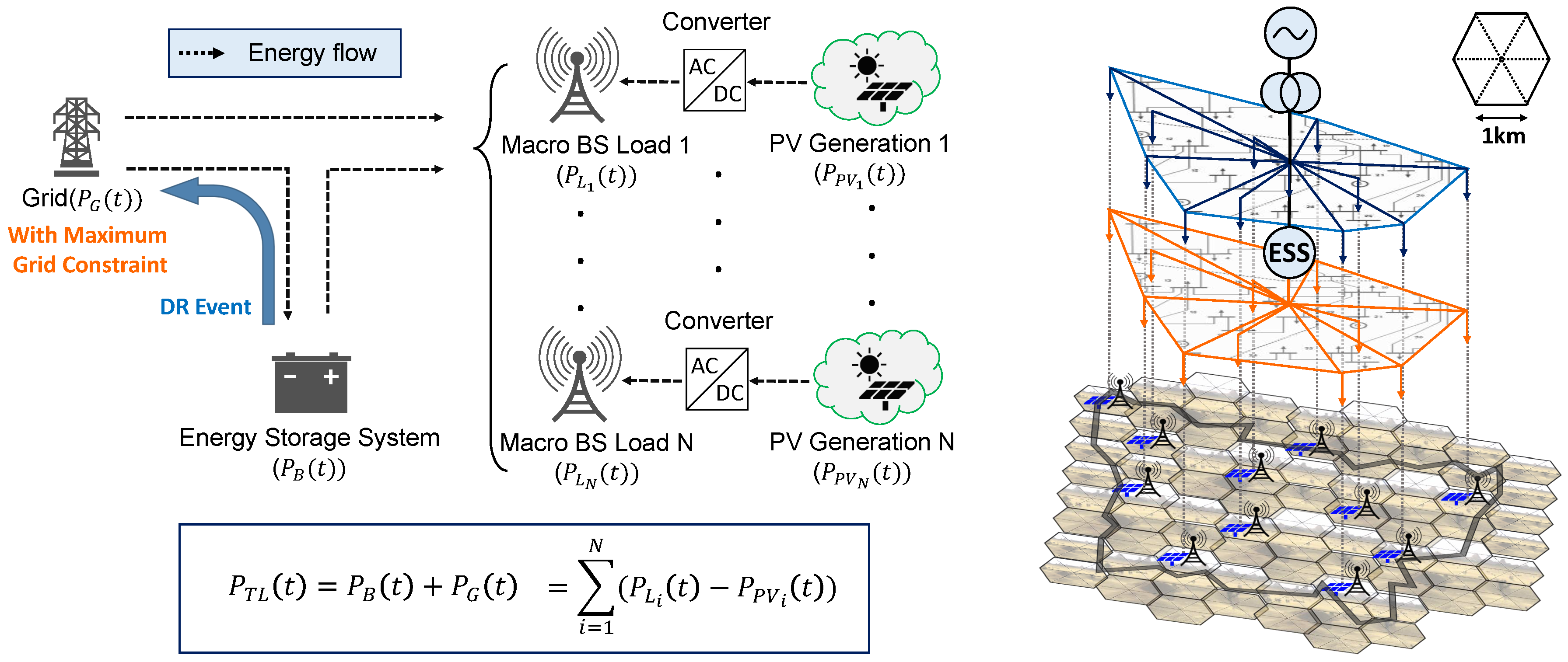
2.1. Sustainable Base Station Model in Smart Grid Environment

We consider a system model for smart grid environment where multiple BSs equipped with PV generators share an ESS and have interoperable connections with the grid as illustrated in Figure 1. We consider macro BSs with hexagonal cell structure, and the PV generator model is with the converter system. Let N be the number of BSs, and each BS is equipped with PV generation facility. We assume that electricity generated by PV resource is firstly used for supporting BS load. The rest of required power is provided by output power of ESS at time t denoted by P B ( t ) , and the power from grid denoted by P G ( t ) . The basic power balance equation then can be represented by P B ( t ) + P G ( t ) = i = 1 N ( P L i ( t ) P PV i ( t ) ) , where i is the BS site index, P L i ( t ) is the load of BS i and P PV i ( t ) is the output power of PV i . Our main objective is to draw an optimal ESS charging and discharging trajectory with minimum operational cost considering battery degradation and multi-functional benefits such as DR, peak shift and TOU, while satisfying power balance equation.

2.2. Power Consumption Model for Macro Base Station

In order to utilize the BS load profile based on real conditions, we consider a general macro BS having multiple transceivers (TRXs), each of which consists of a power amplifier, radio frequency (RF) and baseband unit. BS power consumption also comes from a power supply, a cooling system, and so on [27]. The output power of power amplifier P PA is given by:
P PA = P out η PA ( 1 σ feed )
where P out , η PA and σ feed denote the RF chain output power per transmit antenna, the power efficiency of power amplifier, and the feeder loss, respectively. By using (1), the maximum power consumption of BS P L max is given by [27]:
P L max = N TRX × P PA + P RF + P BB ( 1 σ DC ) ( 1 σ MS ) ( 1 σ cool )
where N TRX is the number of TRX chains, P RF is RF power consumption, P BB is baseband power consumption. σ DC , σ MS and σ cool denote losses incurred by DC-DC power supply, main supply and active cooling system, respectively. The output power derived from (2) is applied to an average daily data traffic profile to extract BS load profile P L ( t ) under the assumption that power consumption is proportional to the BS traffic. The parameter values used in this paper are listed in Table 1.

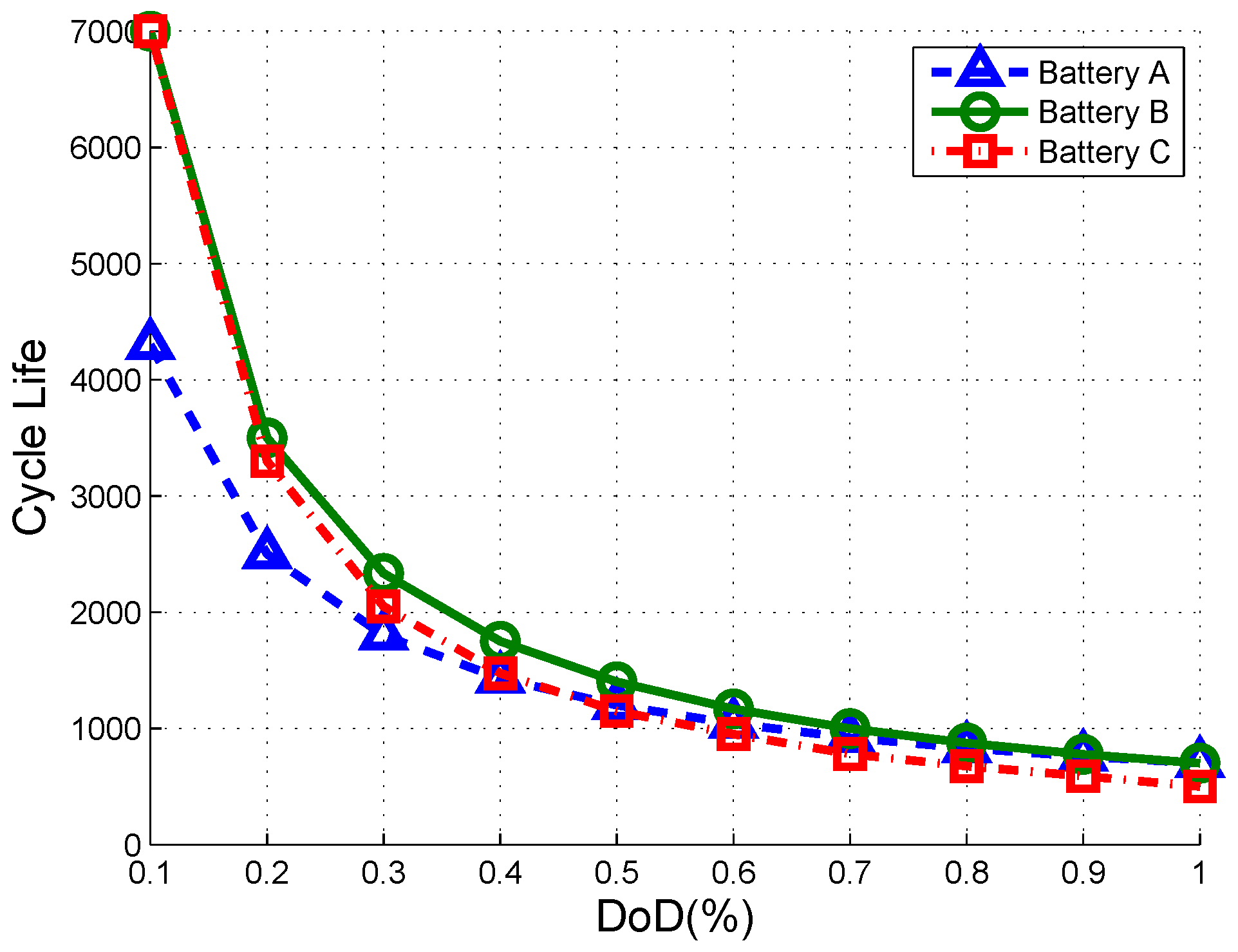
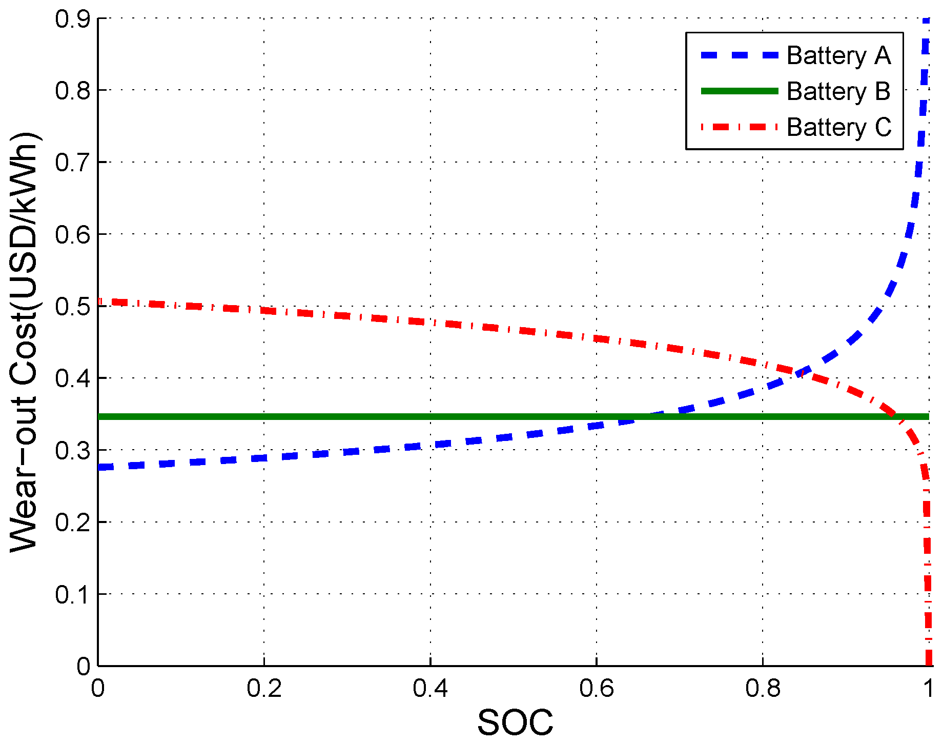
2.3. Battery Wear-Out Model

To capture battery degradation cost, which is critical in minimizing total cost, we leverage the cycle life data; the battery lifetime is measured by the maximum number of charging and discharging cycles, i.e., cycle life. Cycle life is mainly determined by how deeply the battery is used, i.e., DoD. In this work, we consider three types of cycle data obtained from different kinds of batteries, denoted by battery A, B and C. Unlike the cycle life data of battery A and C, which are derived from empirical data sheet of lithium ion battery, battery B is also considered to capture the SOC independent degradation model where cycle life is given exactly by the inverse of DoD with some scaling. Figure 2 shows the cycle life data of battery A, B and C, each of which corresponds to representative battery characteristics as explained below. To capture the battery characteristic, we use the following curve fitting. Typically, numerical curve fittings to given cycle data are modeled by [24]:
N cycle ( D ) = a D b
where D denotes DoD and N cycle is the cycle life. Both a and b are battery specific coefficients, and can be obtained by curve fitting of battery cycle life test data sheet. In [24], wear-out density function W ( s ) is defined as a cost density, where s denotes SOC. Interestingly, battery degradation by using the battery by depth D can be obtainable by integrating W ( s ) , and thus we have:
B a t t e r y p r i c e ( U S D / k W h ) N cycle ( D ) × 2 × D × B a t t e r y c a p a c i t y ( k W h ) × μ 2 = 1 D 1 D 1 W ( s ) d s
where μ denotes the battery efficiency. By differentiating both sides of (4) and substituting (3), the wear-out density function W ( s ) is derived as (5) [24]:
W ( s ) = B a t t e r y p r i c e ( U S D / k W h ) 2 × B a t t e r y c a p a c i t y ( k W h ) × μ 2 × b × ( 1 s ) b 1 a = κ × b × ( 1 s ) b 1 a
In this paper, we note that the parameter b plays an important role in determining the shape of wear-out density function, and that is why we consider three batteries A, B, and C, each of which has a different shape of wear-out density function, as shown in Figure 3. Table 2 summarizes the battery characteristics depending on the range of b. As can be seen, we can classify into three categories; exponentially increasing when b < 1 ; constant when b = 1 ; exponentially decreasing when b > 1 . We will see that the shape of W ( s ) affects the cost and battery lifetime, and provides operational insights observed from several studies.
It should be noted that SOC and state of health (SOH) are indeed related, and to run a charging and discharging algorithm that is dependent on SOC, having proper SOH estimation mechanism is crucial. The history of c-rate, temperature, cell impedance, etc., are important parameters that affect SOH. However, specific SOC or SOH estimation algorithm is beyond the scope of this paper, and thus we assume that SOC and SOH can be reliably estimated at the time of battery operation. Of course, our framework can be combined with other SOC and SOH estimation algorithms when better techniques are available.

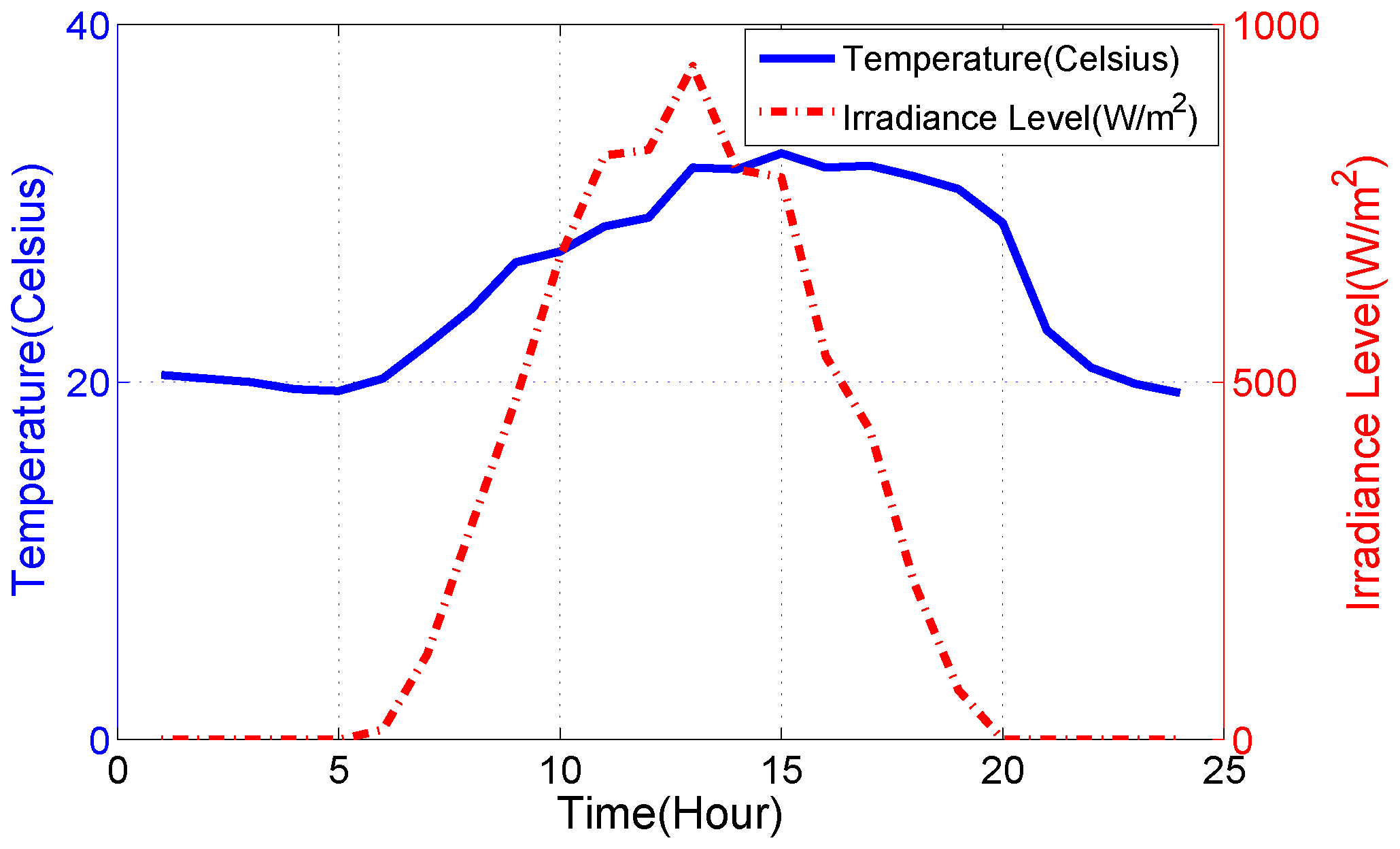
2.4. Photovoltaic Generator Model

Now, we consider the renewable energy source of the BS, i.e., PV generators. The ambient temperature and the solar irradiance level are considered as key components for modeling the output power of PV generation. As shown in Figure 4, we use the average temperature and the irradiance level data of Daegu, Korea on 12 June 2015. Both data are obtained from the Korea Meteorological Administration (KMA), which maintains the official records of all types of national meteorological data. We obtain the output power of PV generation at the maximum power point (MPP) in (6) and (7) as given in [28]:
P PV = P max , ref × G T G T , ref × [ 1 + γ ( T c T ref ) ] × N PV
where P PV denotes the output power of PV at the MPP, and P max , ref is the maximum power in the standard test conditions (STC) and MPP. G T denotes the solar irradiance level on module plane and G T,ref is the incident global irradiance at STC and the reference temperature T ref . In addition, γ , T c and N PV are the temperature factors for power at MPP, the cell temperature and the number of modules, respectively. P max , ref of each module is 200 W, and N PV is six. The cell temperature T c is defined as follows:
T c = T a + G T G NOCT × U L,NOCT U L × ( T NOCT T a,NOCT ) × 1 η c τ α
where T a is the ambient temperature. Normal operating cell temperature (NOCT) is measured under the following environment, i.e., G NOCT = 800 W / m 2 , T a,NOCT = 20 C and the average wind speed of 1 m / s . We assume that normalized thermal loss coefficient U L,NOCT / U L is equal to one, and η c / τ α is also much less than one. The rest of parameter values are as in [29].

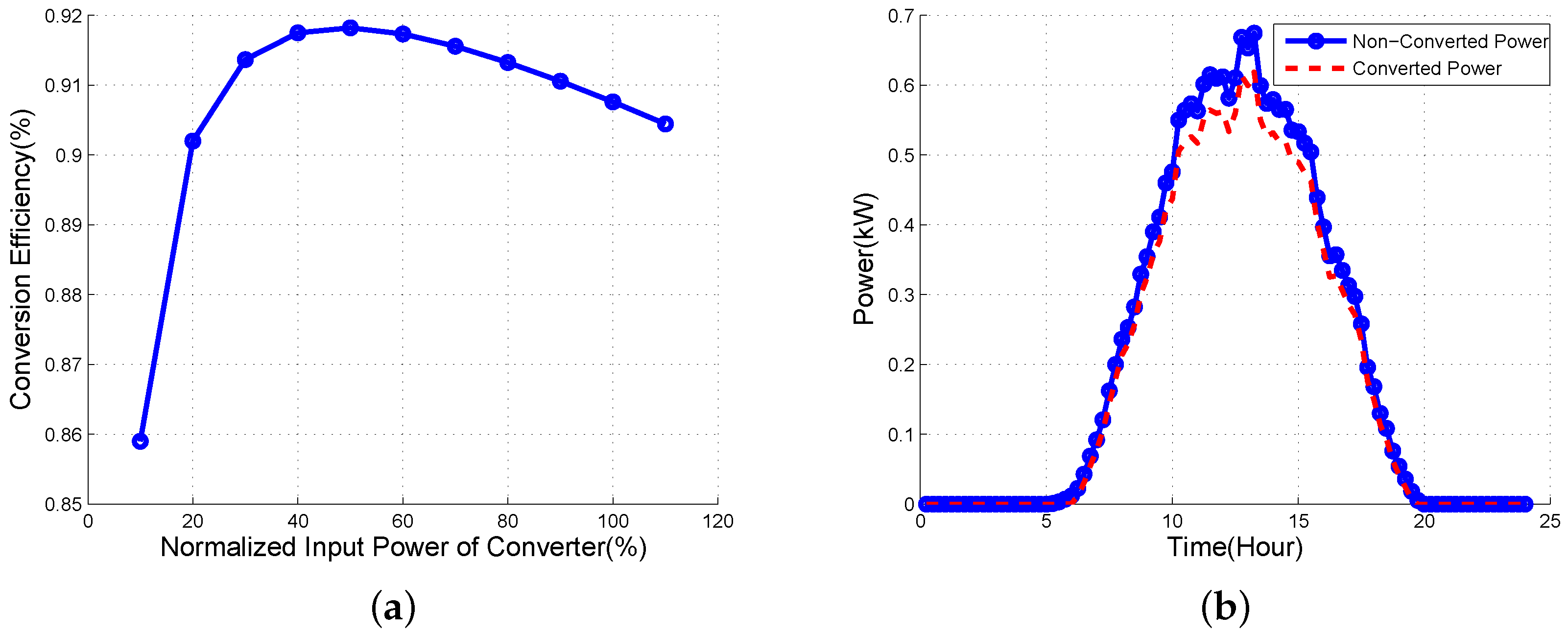
2.5. Converter System Model

Converter system plays an important role in the power system connected with PV since it converts DC output from PV into AC output that can be fed into the grid or support the load directly. The function for conversion efficiency η conv can be expressed in this quadratic form as (8) given in [29]:
η conv = 1 P rated P in × 0 . 0094 + 0 . 043 × P rated P in + 0 . 04 × P rated P in 2
where the normalized input power of converter is defined by the rated power of converter P rated over the input power P in . Figure 5b describes the sample of PV output power profile during 24 h after converting shown in Figure 5a.

3. Multi-Functional Energy Storage System Optimization
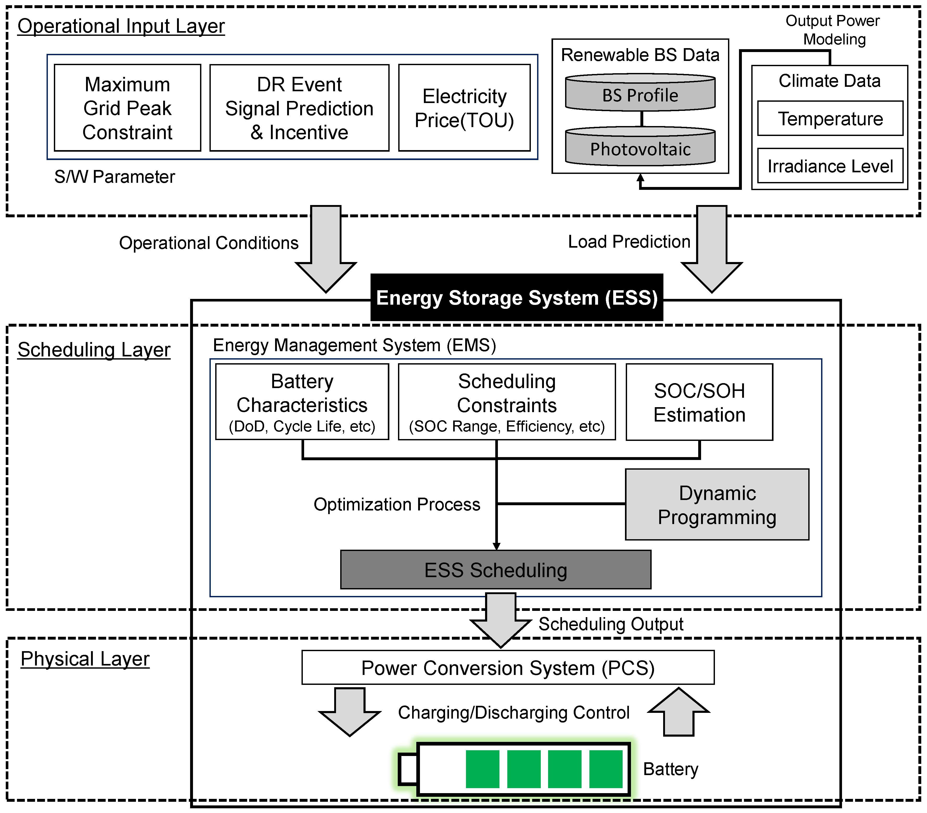
In this section, we formulate an optimization problem based on the models in Section 2 and present a solution based on DP. Furthermore, multi-functions for peak shift, DR and TOU will be described. The proposed framework has three layers: operational input layer, scheduling layer, and physical layer as illustrated in Figure 6:
(1)
Operational input layer: This layer consists of multi-functional objective and load calculation parts. The multi-functional objective part consists of peak shift, DR and TOU for maximizing economic profit. In load calculation, renewable output power is calculated by applying PV output power modeling and convert system based on the average temperature and irradiance level data. Then, through a power consumption model for macro BS, total required BS load is finally calculated. Operational conditions and load prediction data base are delivered from this layer to the scheduling layer.
(2)
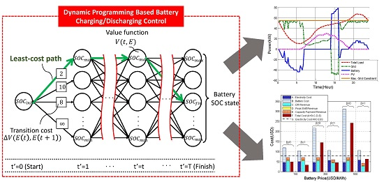
Scheduling layer: Using DP, optimization is performed to obtain the ESS scheduling by combining the operating conditions and load prediction data with the measured battery characteristics, scheduling constraints and SOC/SOH estimation. The scheduling layer transfers the optimized scheduling output to the physical layer for operating ESS by charging and discharging.
(3)
Physical layer: Based on the scheduling result from the scheduling layer, the power conversion system (PCS) performs practical ESS charging and discharging.

3.1. Multi-Functional Framework Using Dynamic Programming

The optimization of ESS scheduling is to obtain the charging and discharging path having the minimum value function V ( t , E ) in (9), where t T is the discrete time index, T = { 1 , , T } and E is the energy state, i.e., the stored energy in the battery. We split V ( t , E ) into two parts, the operational cost denoted by U ( t , E ) from a certain discrete time t to end time T, and the battery wear-out cost arising from charging and discharging, denoted by W ( t , E ) . Then, U ( t , E ) and W ( t , E ) are combined by the weighting parameter β to control the trade-off between operational cost and battery wear-out cost, and thus we have:
V ( t , E ) = U ( t , E ) + β W ( t , E )
The operational cost U ( t , E ) is given by:
U ( t , E ) = t = t T ( P G ( t ) C ( t ) 1 { P G ( t ) 0 } P B ( t ) D ( t ) 1 { D R is activated } ) Δ t
where C ( t ) is TOU electricity price as will be explained in Section 4.1. 1 { } is an indicator function returning 1 if the condition is true, and 0 otherwise. P B ( t ) is the output power of battery (positive when discharging and negative when charging), D ( t ) is the DR incentive price, and Δ t is the unit time interval. DR incentive allows operators to reduce electricity consumption voluntarily by providing beneficial incentive. The second term in (10) is for achieving economic profit from DR incentive by discharging ESS.
The battery wear-cost W ( t , E ) is given by:
W ( t , E ) = t = t T C B ( E ( t ) , E ( t + 1 ) )
where C B ( E ( t ) , E ( t + 1 ) ) in (11) is the battery wear-out cost when the stored energy in the battery changes from E ( t ) to E ( t + 1 ) . As mentioned in Section 2, battery degradation can be calculated by integrating the wear-out density function W ( s ) as in (12):
C B ( E ( t ) , E ( t + 1 ) ) = E ( t ) E max E ( t + 1 ) E max W ( s ) d s
where E max is the rated battery capacity. Note that (12) is one specific realization to capture battery degradation, and our frame based on DP can be combined with other battery degradation models as long as they are state-dependent.
Then, the state transition cost from the state ( t , E ( t ) ) to ( t + 1 , E ( t + 1 ) ) is given by:
Δ V ( E ( t ) , E ( t + 1 ) ) = ( P G ( t ) C ( t ) 1 { P G ( t ) 0 } P B ( t ) D ( t ) 1 { D R is activated } ) Δ t + β C B ( E ( t ) , E ( t + 1 ) )
By using this state transition cost and satisfying the power and energy constraints of (16) to (20), we calculate the value function V ( t , E ) for every t and E:
V ( t , E ) = min E ( t + 1 ) { Δ V ( E , E ( t + 1 ) ) + V ( t + 1 , E ( t + 1 ) ) }
by solving the Bellman equation. The process starts at t = T where the value function has zero value and goes backward until reaching the initial time. This results in determining the least cost path for every possible energy state at every time step. Then, we construct a total charging and discharging path by forward induction:
E * ( t ) = argmin E ( t ) { Δ V ( E * ( t 1 ) , E ( t ) ) + V ( t , E ( t ) ) }
with some given initial condition E * ( 0 ) , and we finally have an optimal energy state E * ( t ) at every t. Note that during all the steps, the following constraints must be satisfied for every t:
P G ( t ) + P B ( t ) = P TL ( t )
P TL ( t ) = i = 1 N ( P L i ( t ) P P V i ( t ) )
P B ( t ) = E ( t ) E ( t + 1 ) Δ t
S O C min E ( t ) E max S O C max
P B ( t ) P B max
where P TL ( t ) is total net load of all BSs. We assume that P TL ( t ) can be obtainable in a reasonably accurate way by using, for example, machine learning techniques based on historical learning data, which is beyond the scope of this paper. S O C min and S O C max are the minimum and maximum SOC requirements, E max is the rated battery capacity, P B max is the maximum charging and discharging rate of battery, and P G max is the maximum grid power constraint. Note that the constraints (19) and (20) can be easily implemented in DP by properly assigning the state transition costs depending on the energy state E ( t ) and the difference between two energy states E ( t ) and E ( t + 1 ) , respectively. By carrying out the all the equations and constraints we have set, DP can provide a globally optimal solution.

3.2. Peak Shift

Peak shift is one of the essential functions of ESS to stabilize the grid when the grid needs to restrict peak demand under certain constraint. Furthermore, peak shift can significantly reduce the base electricity cost, which is determined by the yearly highest load of 15 min, for example, in Korea. Thus, sustaining the peak load under some target P G max is important from both grid stability and economic perspectives, and we are motivated to include a peak shift algorithm along with TOU in the same framework. Note that, so far, ESS scheduling algorithms focus on either TOU or peak shift, but not both at the same time. Given the net load profile P TL ( t ) , sustaining the net load below P G max can be done by satisfying the following constraint for t T :
P G ( t ) = P TL ( t ) P B ( t ) P G max
Using DP, (21) can be easily implemented as follows. For any given state transition from ( t , E ( t ) ) to ( t + 1 , E ( t + 1 ) ) , we augment the state transition cost Δ V ( E ( t ) , E ( t + 1 ) ) in (13) by C peak × ( P G ( t ) P G max ) if (21) is violated. If C peak is set as , then peak shift becomes the most critical and (21) must be satisfied as long as that is feasible. The algorithm is summarized as follows:
Algorithm Peak Shift
Input: P TL ( t ) , P G max , E max and C peak
Output: Δ V ( E ( t ) , E ( t + 1 ) )
  1:
procedure peak shift 
  2:
    set E max as an effective value with respect to P G max  
  3:
    for t = T to 1 do 
  4:
        if P G ( t ) P G max then 
  5:
           transition cost Δ V ( E ( t ) , E ( t + 1 ) ) is computed as in (13) 
  6:
        else 
  7:
           transition cost Δ V ( E ( t ) , E ( t + 1 ) ) Δ V ( E ( t ) , E ( t + 1 ) ) + C peak × ( P G ( t ) P G max )  
  8:
        end if 
  9:
    end for 
10:
end procedure

4. Experimental Results from Operational Scenarios

In this section, based on the aforementioned algorithms, we present three representative case studies and also analyze the performance in terms of an economic perspective and battery life extension under different operational conditions.

4.1. Experimental Set-Up

Figure 7 shows sample profiles of 50 macro BS loads and PV generations that have deviation of ±5%, respectively. Since we consider a system model where multiple BSs equipped with PV generators share an ESS, we intend to take into account the realistic measured value about load and generation varying depending on the location. The highest peak of BS load curve is during the evening, while that of PV generation is in the middle of the afternoon. Since ESS charge and discharge energy loss is dominant compared with the distribution line loss [30], overall energy loss of ESS system is set to 15% of the rated battery capacity, i.e., efficiency of ESS system is 0.85. All available load data in this paper are taken every 15 min over one day (24 h). Following this, time step in our simulation is 15 min, and we have 96 time steps during 24 h. As can be seen from Figure 8, we utilize the practical day-ahead electricity price from California ISO (CAISO), which has $0.14/kWh as highest price and $0.04/kWh as lowest price in this paper [12]. Battery SOC stays within preset upper and lower limits (upper = 0.9, lower = 0.1) to prevent suffering from high stress at both ends of the SOC; this is widely adopted in the lithium-ion battery industry. The rest of the parameters used in the simulations are summarized in Table 3.

4.2. Case Study

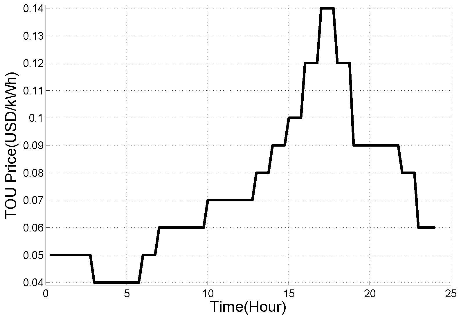
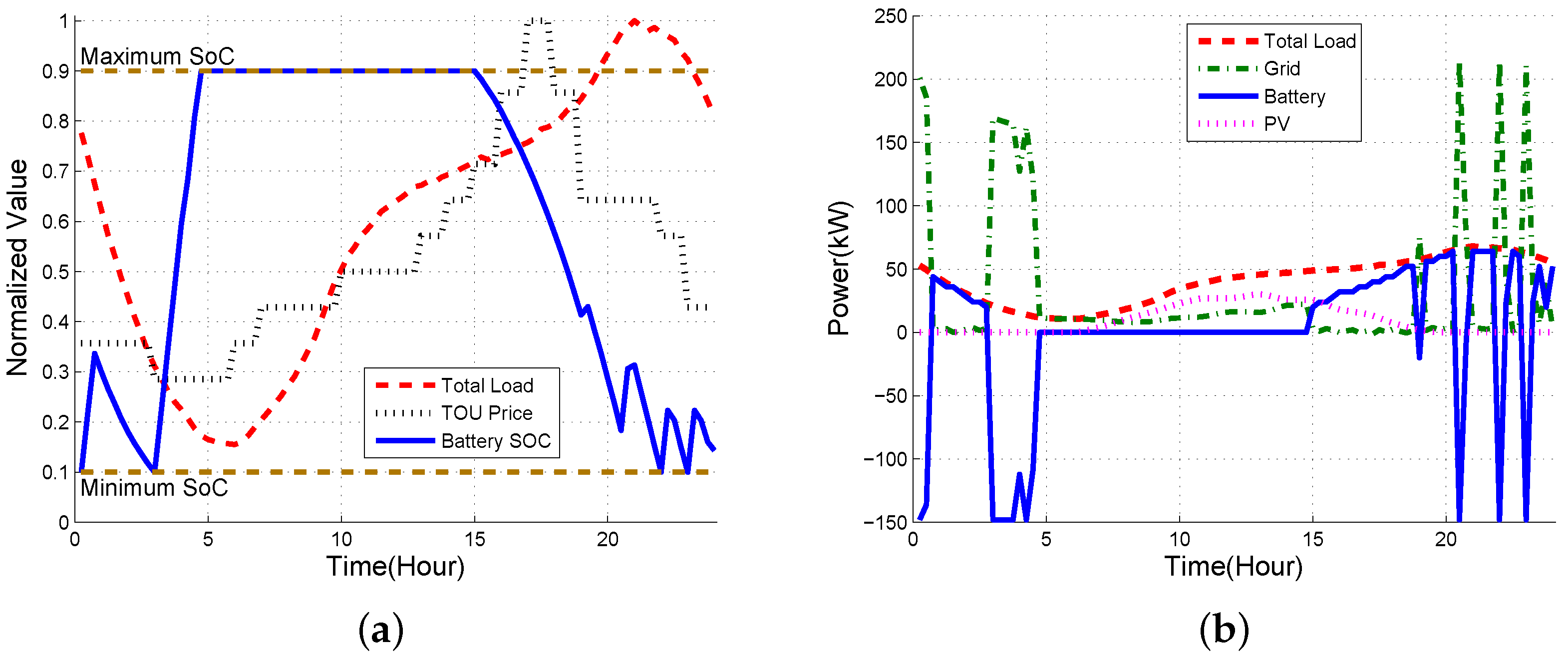
4.2.1. Case 1: Basic Dynamic Programming with Time of Use Only

Figure 9 shows the results of basic optimal scheduling when TOU is considered, but without considering DR, peak shift and battery wear-out. Since battery wear-out is not reflected in the optimal scheduling computation, the operator can only benefit from the difference between TOU tariffs. Thus, we observe that charging and discharging enables the operator to get a profit from a TOU tariff regardless of battery degradation, even if several peaks occur over a high demand period. Note that since battery wear-out is not considered in Case 1, DP may choose the charging and discharging path out of several equal cost paths when a tie occurs, which may lead to unnecessary frequent charging and discharging unless a deliberate tie-breaking rule is included. We will see that our solution considering battery wear-out in Case 3 does not have this issue.
As can be seen from Figure 9a, the ESS fully stores energy from the main grid when the electricity price is the lowest (3 a.m. to 6 a.m.) and consumes the stored energy to support the required BS load when the electricity price is relatively high. In Figure 9b, note that the maximum power from grid (green dash-dot line) is nearly three times higher than that of the required BS load (red dashed line). From the economic perspective, the electricity cost per day without ESS is $79.7, but it costs $43.8 by using DP method with ESS, and thus it was reduced by 45.0%. We use the net metering for calculation of electricity cost based on the TOU as described in Figure 8. However, this electricity cost reduction comes from excessive battery usage, i.e., at the expense of battery degradation. To quantify battery usage, we define the battery usage as the ratio of battery degradation compared to that of one charging and discharging cycle between minimum and maximum SOC. For example, if the battery experiences one full charge and discharge between maximum and minimum SOC, the battery usage is one. The battery usage in Case 1 turns out to be 1.79.

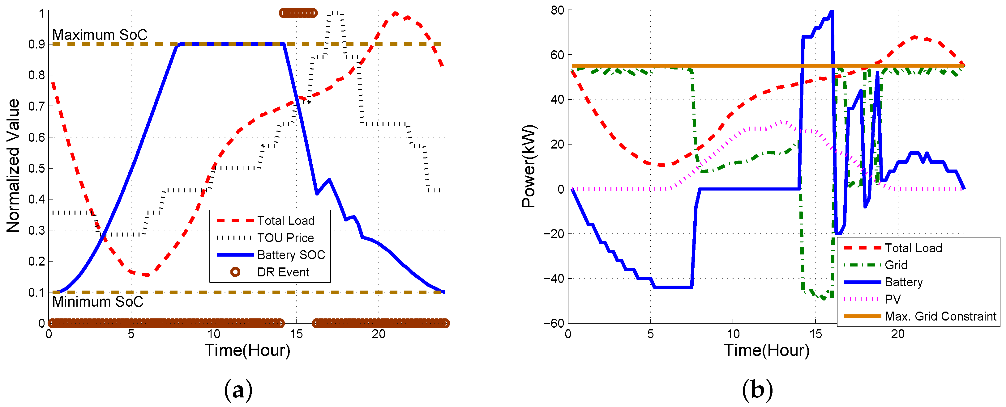
4.2.2. Case 2: Multi-Functional Dynamic Programming without Considering Battery Wear-Out

The next case is the same as Case 1 except for including DR and peak shift to improve economic profit and guarantee the power limit from the grid. Unlike the previous case showing that the ESS charges sharply during the lowest TOU price period (3 a.m. to 6 a.m.), the ESS in Case 2 has a smooth trajectory to prevent P G ( t ) from exceeding P G max as can be seen in Figure 10. This is because the algorithm compares the benefit from TOU tariff and the penalty when P G ( t ) goes over P G max . In the simulation, we set C peak = , i.e., peak load must not exceed P G max . Meanwhile, assuming that DR incentive has been applied as one of the multi-functions during the period when DR event signal is activated (2 p.m. to 4 p.m.), the operator can get an economic profit by the amount of power reduction during this period as well as the capacity payment ($53.7 and $13.4, respectively). To get a profit during the highest TOU period which follows the DR, the ESS charges and discharges a small amount of electricity. After that, peak shift starts at 18:30 PM continuing for five and half hour, which saves the base electricity bill by the amount of peak reduction ($3.6) from following equation:
R PS ( per day ) = ( P TL max P G max ) × $ 8 . 3 / k W 30 day
A monthly base electricity bill is calculated by the measured highest peak during summer and winter season in a year, i.e., July, August, September, December, January and February, including the month of measuring. It is based on the industrial B type, high-voltage A type with option 2 electricity tariff in the summer season of the Korea Electric Power Corporation (KEPCO) and fixed for one year.
Comparing Case 1 and Case 2, the electricity cost in Case 2 increases by 7.4%, but the battery wear-out cost decreases by 36.9%; the battery usage also decreases by 40.2%. As a result, we observe that drastic changes of power and frequent switchings of charging and discharging are clearly reduced compared with Case 1 in Figure 9.

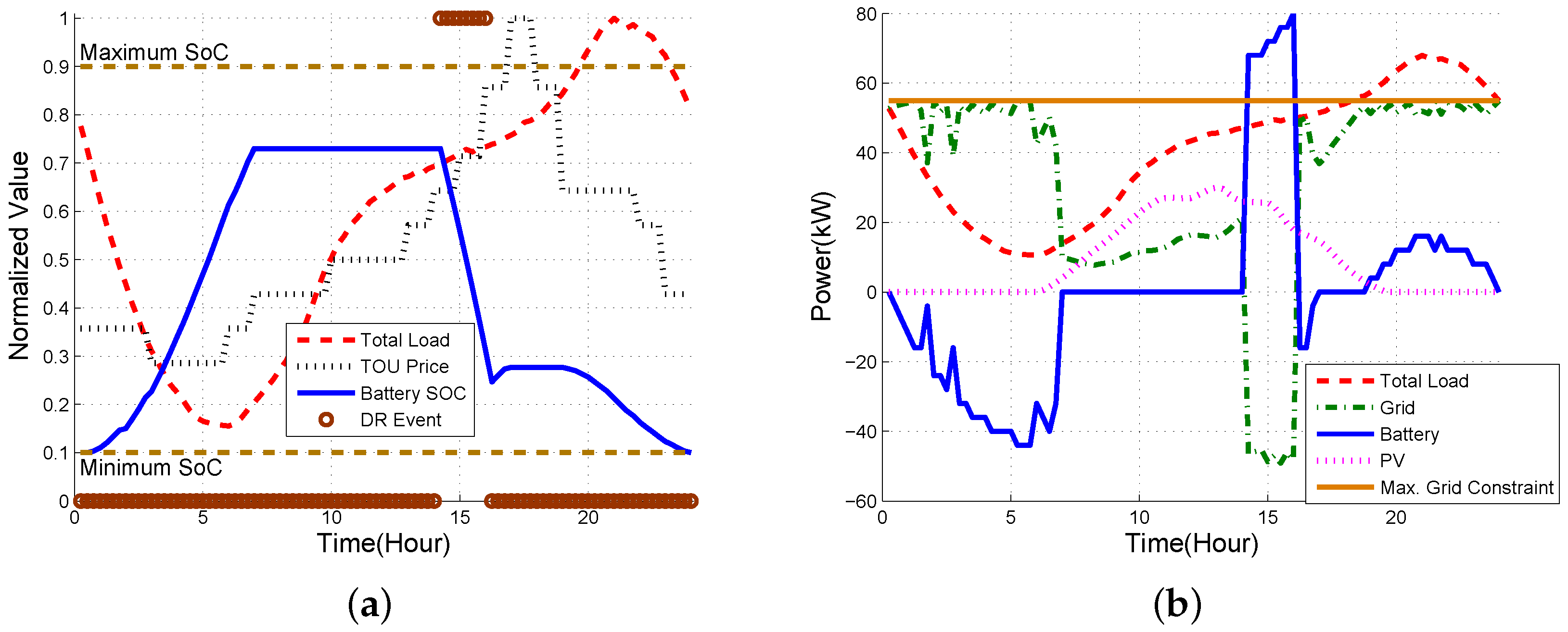
4.2.3. Case 3: Multi-Functional Dynamic Programming with Battery Wear-Out Model

In Figure 11, we investigate the effect of the multi-functional DP with battery wear-out model. The results of Case 3 differs from that of Case 2 as follows. First, SOC reaches only up to 0.73 because, beyond that point, the profit from TOU would be less than the cost from the battery wear-out. Note that the wear-out function of battery A rises sharply after 0.7 SOC, as can be seen in Figure 3. Second, unlike Case 2, Case 3 does not have frequent charging and discharging processes after the DR event. This is to reduce the battery cost caused by the changes of battery SOC. As a result, although the electricity cost increases by 8.5%, the total cost decreases by 28.7%. This is mainly due to the reduced battery cost, i.e., 27.0% lower than that of the Case 2. The total cost considering electricity cost, battery cost, DR revenue ( R DR ), capacity revenue ( R cap ), peak shift revenue ( R PS ) is given by:
C total = C elec + C batt R DR R cap R PS
and Table 4 summarizes all the results for Case 1, 2 and 3. Table 4 shows that, if the multi-function with the battery wear-out exists in ESS, the overall system cost is reduced by up to 70.6% compared to Case 1. Note that the battery usage is reduced by up to 53.6%, and it is obvious that battery cost is critical in determining the cost and battery usage in ESS operation.

4.3. Performance Evaluations

In this subsection, we focus on how the performance of our proposed approach varies with parameters, e.g., weighting factor, battery price and maximum grid constraint. Specifically, we present in detail that considering wear-out has an important role in ESS operation through the analysis of cost and battery usage as the weighting factor β varies.

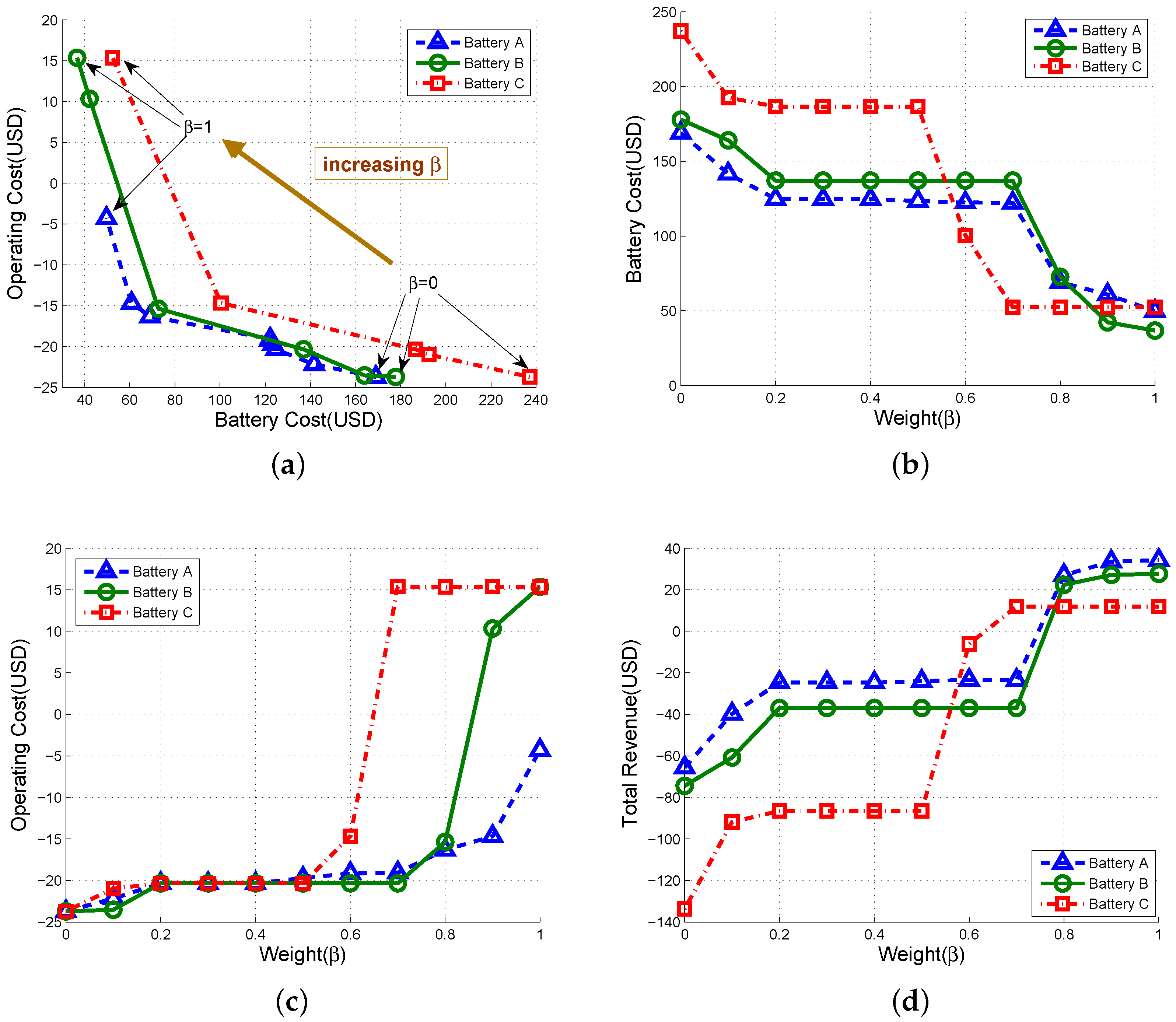
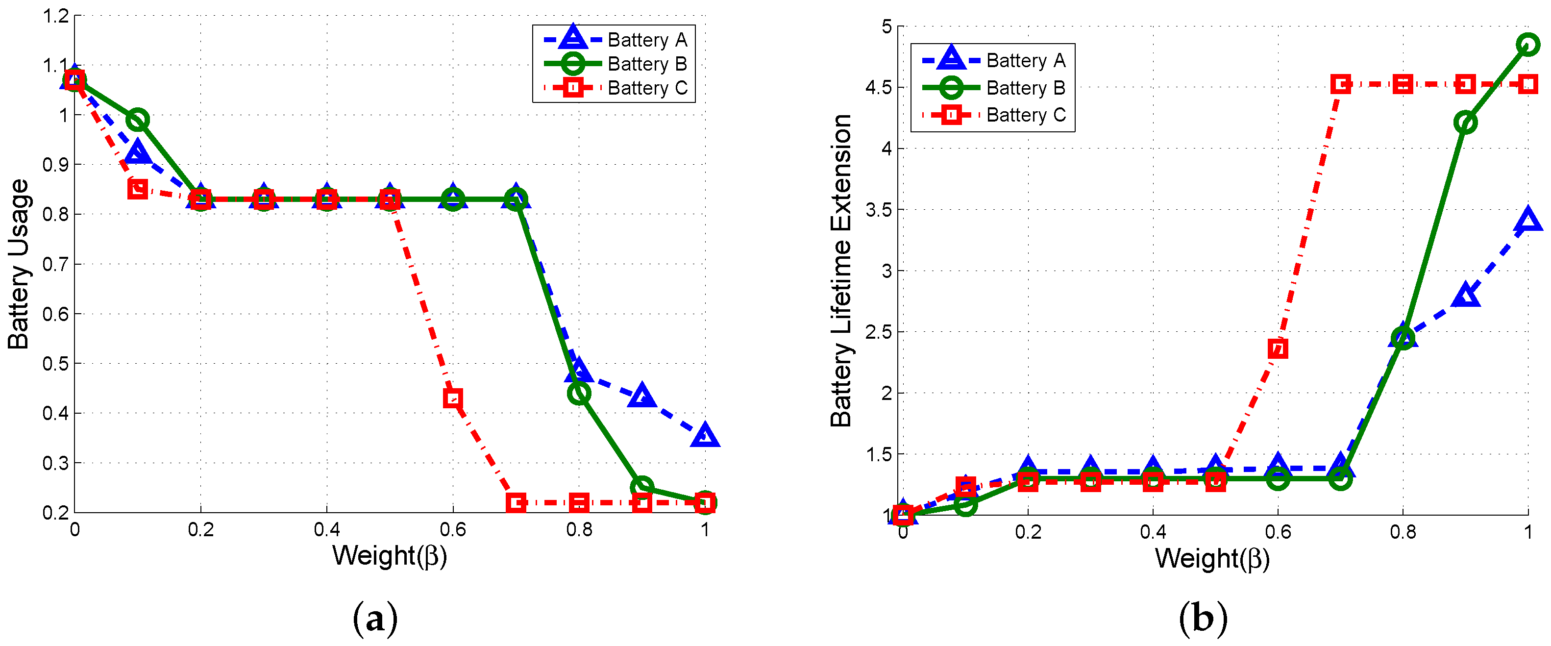
4.3.1. Trade-Off between the Operating Cost and the Battery Cost

Note that the parameter β in (9) determines how much the operator cares about battery degradation. If β = 0 , the operation is oblivious to battery cost. If β = 1 , the operator fully acknowledges battery degradation. In Figure 12a, as β changes from 0 to 1, we plot the operational cost and the battery cost; the battery cost generally decreases as β grows while the operating cost C oper given by (24) increases:
C oper = C total C batt = C elec R DR R cap R PS
This is because if we focus more on battery degradation by increasing β , the transition cost calculated by the wear-out function increases. Thus, the scheduler tries to suppress the battery usage, which results in increasing the operating cost. Consequently, there is a trade-off between the operating cost and the battery cost as shown in Figure 12b,c.
In Figure 12d, we plot the revenue of using multi-functional ESS, which is defined in (25) as the cost difference before and after using ESS:
R total = C conv,elec C total = C conv,elec C elec + R DR + R cap + R PS C batt
where C conv,elec denotes the electricity cost when ESS is not used. As can be seen, as β becomes larger, the revenue significantly increases. For all battery types, we see that positive revenue is possible when β is 0.8 or more. Total revenues are in order of battery A, B and C when β is one, i.e., $34.28, $27.68 and $11.97, which is related to the shape of wear-out function. Interestingly, battery C’s revenue increases sharply around β = 0 . 6 since the scheduler restricts the use of the battery when β is 0.6 or more (high wear-out cost), which is also demonstrated in Figure 12b.
We further investigate the battery usage depending on the weighting factor β , and there are two observations. First, as expected, higher β contributes to decreasing battery usage as in Figure 13a and the battery usage is in order of battery A, B, and C in general. This is because, by integrating the wear-out function over the same SOC period, wear-out cost is mostly in order of battery C, B, and A. As a result, the battery usage becomes inversely proportional to the calculated battery wear-out, and then the reduction of battery usage from β = 0 to β = 1 is 67.3%, 79.4% and 79.4% for battery A, B and C, respectively.
Next, Figure 13b shows the relation between β and the battery lifetime extension, which is defined as B L ( β ) B L ( 0 ) where B L ( β ) is defined in (26) such as:
B L ( β ) = B a t t e r y c a p a c i t y ( kWh ) × B a t t e r y p r i c e ( USD/kWh ) D a i l y b a t t e r y w e a r o u t ( β ) ( USD )
The implication of battery lifetime extension (BLE) is related to how long we can use the battery compared to the case of β = 0 . As expected, lifetime is extended as β increases. It is interesting to see that the lifetime of batteries A and B are noticeably extended after β is 0.7, and the lifetime of battery C is extended sharply after β = 0 . 5 and saturates at β = 0 . 7 . Finally, when β = 1 , the lifetime is substantially extended by 3.4, 4.8 and 4.5 times for battery A, B and C, respectively.

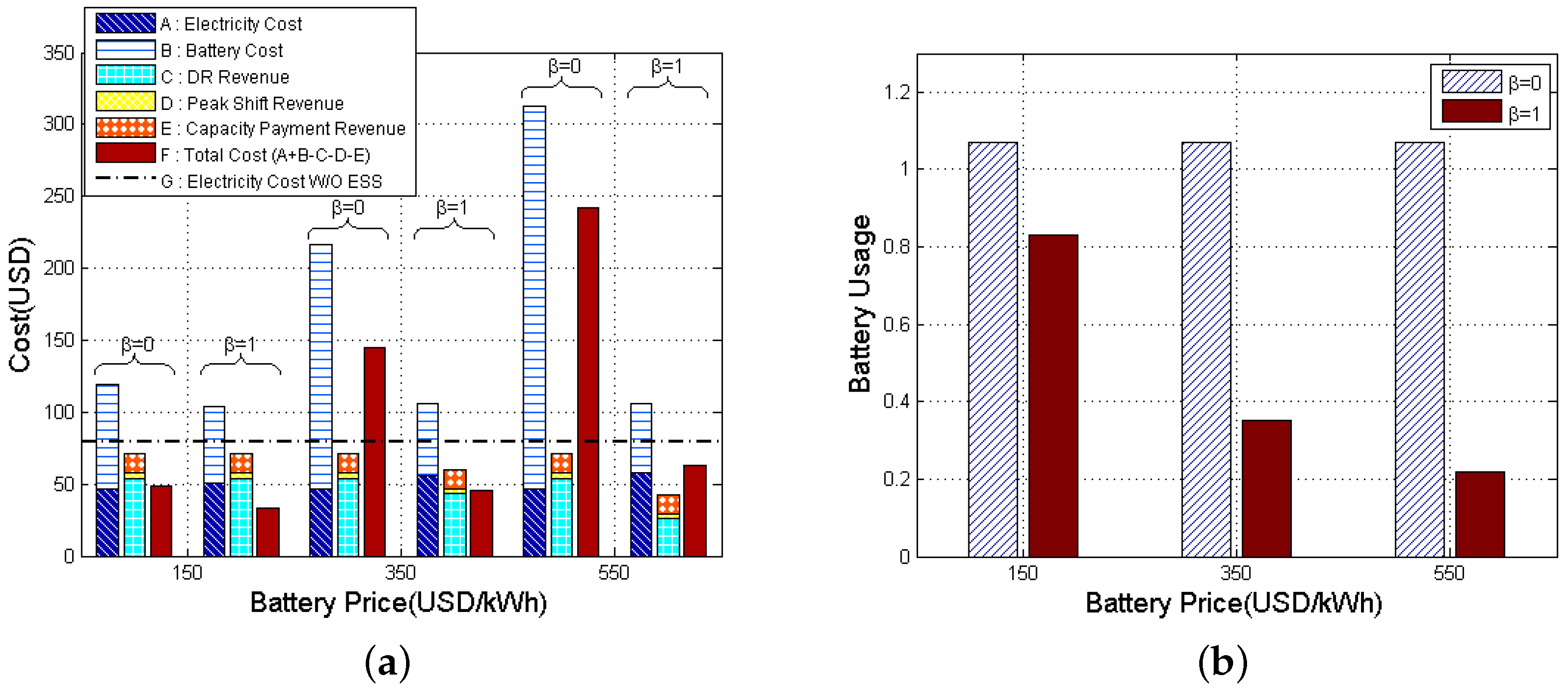
4.3.2. Cost Analysis with Battery Usage and Prices

Now, we analyze the total cost depending on the battery usage and battery price. Figure 14a compares the costs in detail for different battery prices ($150/kWh, $350/kWh and $550/kWh) and with/without wear-out consideration ( β = 0 or 1) for the case of battery A. In each case, three bars consist of various costs or revenues as follows: electricity cost (A), battery cost (B), DR revenue (C), peak shift revenue (D), capacity payment revenue (E) and total cost (F = A + B − C − D − E). The electricity cost without ESS (G), which appears in (25) as C conv,elec , is denoted by the horizontal dash-dot line. Thus, if total cost (F) is below G, using ESS is beneficial, and vice versa. We can see that when battery price is $350/kWh or $550/kWh, β = 0 exhibits excessive battery cost, and using ESS is economically disadvantageous. However, the case of β = 1 substantially reduces battery cost while DR revenue loss and electricity cost increase are both negligible. Consequently, the total cost decreases significantly compared to the case of β = 0 , which shows the benefit of the proposed solution. In Figure 14b, we observe that the battery usage in the case of β = 1 significantly decreases as the battery price increases. Comparing with the case of β = 0 , battery usage is reduced by 22.4%, 67.3% and 79.4% for the battery price, $150/kWh, $350/kWh and $550/kWh, respectively.

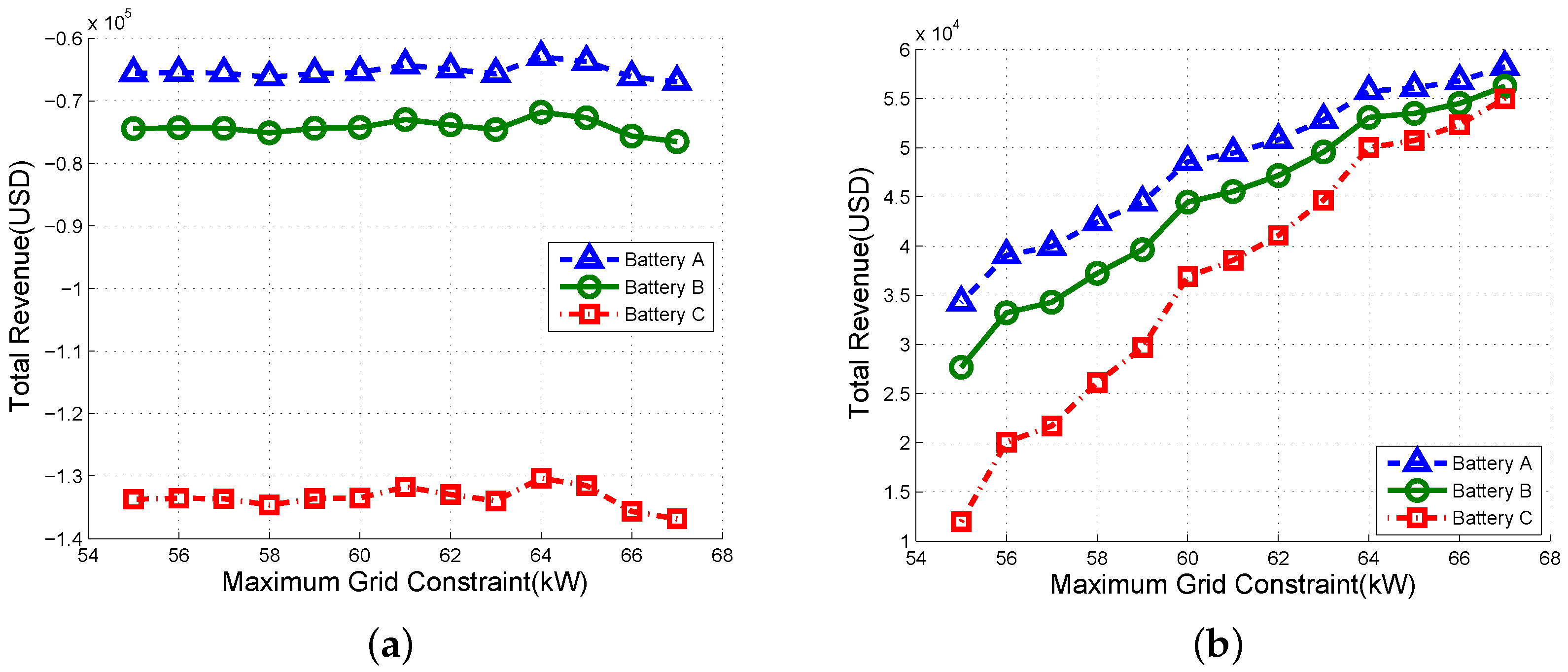
4.3.3. Maximum Grid Constraint and Total Revenue

Figure 15 shows the total revenue with maximum grid constraints P G max for three kinds of batteries. In Figure 15a, the ESS is fully utilized to maximize profits from TOU, DR and peak shift, and this results in increased battery cost. As a result, we observe that total revenue is always negative regardless of P G max if battery wear-out is not considered. Figure 15b shows that the total revenue increases in order of battery A, B and C as P G max increases. This is due to decreasing of reserved capacity for peak shift resulting in low battery cost, and this leads to positive total revenue. In particular, we verify that total revenue is inversely proportional to the value of wear-out function as can be seen in Figure 3.

5. Conclusions

In this paper, we have proposed a novel framework for multi-functional ESS scheduling to minimize total operational cost of sustainable BS using DP optimization. In designing the strategy, we have considered practical sustainable BS environments, i.e., PV generators, converters and BS load as well as detailed battery wear-out models based on realistic data. Multi-functioning of ESS includes DR, peak shift and TOU to get the most profit and guarantee the maximum peak constraint as well. Our scenario-based simulations have demonstrated that the proposed approach significantly reduces the total cost and battery usage by up to 70.6% and 53.6%, respectively, compared to the conventional method without considering battery wear-out. Furthermore, from the trade-off between the operating cost and battery cost, we have verified that battery usage can be controlled by adjusting the weighting factor β from zero to one, and this results in prolonging battery lifetime by up to almost five times. Our approach is general and thus applicable to other applications and load types as well, such as office buildings, large-scale residential complexes and factories, etc., where the electricity consumption pattern is periodic usually. Our work can be further extended by considering a battery model in terms of electrochemistry that focuses on temperature change in particular. Considering temperature can model more accurate battery wear-out since cell degradation is easily affected by temperature change.

Acknowledgments

This work was supported in part by the Basic Science Research Program through the National Research Foundation of Korea (NRF) funded by the Ministry of Science, ICT and Future Planning under Grant NRF-2014R1A1A1006551.

Author Contributions

Yohwan Choi designed the algorithm, performed the simulations, and prepared the manuscript as the first author. Hongseok Kim led the project and research. All authors discussed the simulation results and approved the publication.

Conflicts of Interest

The authors declare no conflict of interest.

References

  1. Piro, G.; Miozzo, M.; Forte, G.; Baldo, N.; Grieco, L.A.; Boggia, G.; Dini, P. Hetnets powered by renewable energy sources: Sustainable next-generation cellular networks. IEEE Internet Comput. 2013, 17, 32–39. [Google Scholar] [CrossRef]
  2. Issaadi, W.; Khireddine, A.; Issaadi, S. Management of a base station of a mobile network using a photovoltaic system. Renew. Sustain. Energy Rev. 2016, 59, 1570–1590. [Google Scholar] [CrossRef]
  3. Zordan, D.; Miozzo, M.; Dini, P.; Rossi, M. When telecommunications networks meet energy grids: Cellular networks with energy harvesting and trading capabilities. IEEE Commun. Mag. 2015, 53, 117–123. [Google Scholar] [CrossRef]
  4. Aris, A.M.; Shabani, B. Sustainable Power Supply Solutions for Off-Grid Base Stations. Energies 2015, 8, 10904–10941. [Google Scholar] [CrossRef]
  5. Sui, X.; Tang, Y.; He, H.; Wen, J. Energy-storage-based low-frequency oscillation damping control using particle swarm optimization and heuristic dynamic programming. IEEE Trans. Power Syst. 2014, 29, 2539–2548. [Google Scholar] [CrossRef]
  6. Ye, Y.; Jimenez Arribas, F.; Elmirghani, J.; Idzikowski, F.; Lopez Vizcaino, J.; Monti, P.; Musumeci, F.; Pattavina, A.; Van Heddeghem, W. Energy-efficient resilient optical networks: Challenges and trade-offs. IEEE Commun. Mag. 2015, 53, 144–150. [Google Scholar] [CrossRef]
  7. Wang, C.X.; Haider, F.; Gao, X.; You, X.H.; Yang, Y.; Yuan, D.; Aggoune, H.; Haas, H.; Fletcher, S.; Hepsaydir, E. Cellular architecture and key technologies for 5G wireless communication networks. IEEE Commun. Mag. 2014, 52, 122–130. [Google Scholar] [CrossRef]
  8. Public Utilities Code Section 2835–2839; State of California: USA, 2010. Available online: http://www.leginfo.ca.gov/cgi-bin/displaycode?section=puc (accessed on 1 January 2011).
  9. Soroudi, A.; Siano, P.; Keane, A. Optimal DR and ESS Scheduling for Distribution Losses Payments Minimization Under Electricity Price Uncertainty. IEEE Trans. Smart Grid 2016, 7, 261–272. [Google Scholar] [CrossRef]
  10. Tan, Z.; Li, H.; Ju, L.; Song, Y. An Optimization Model for Large-Scale Wind Power Grid Connection Considering Demand Response and Energy Storage Systems. Energies 2014, 7, 7282–7304. [Google Scholar] [CrossRef]
  11. Grillo, S.; Marinelli, M.; Massucco, S.; Silvestro, F. Optimal management strategy of a battery-based storage system to improve renewable energy integration in distribution networks. IEEE Trans. Smart Grid 2012, 3, 950–958. [Google Scholar] [CrossRef]
  12. Shi, W.; Xie, X.; Chu, C.C.; Gadh, R. Distributed optimal energy management in microgrids. IEEE Trans. Smart Grid 2015, 6, 1137–1146. [Google Scholar] [CrossRef]
  13. Pudjianto, D.; Aunedi, M.; Djapic, P.; Strbac, G. Whole-systems assessment of the value of energy storage in low-carbon electricity systems. IEEE Trans. Smart Grid 2014, 5, 1098–1109. [Google Scholar] [CrossRef]
  14. Yang, H.; Chung, C.; Zhao, J. Application of plug-in electric vehicles to frequency regulation based on distributed signal acquisition via limited communication. IEEE Trans. Power Syst. 2013, 28, 1017–1026. [Google Scholar] [CrossRef]
  15. Levron, Y.; Guerrero, J.M.; Beck, Y. Optimal power flow in microgrids with energy storage. IEEE Trans. Power Syst. 2013, 28, 3226–3234. [Google Scholar] [CrossRef]
  16. Armand, M.; Tarascon, J.M. Building better batteries. Nature 2008, 451, 652–657. [Google Scholar] [CrossRef] [PubMed]
  17. Zhou, C.; Qian, K.; Allan, M.; Zhou, W. Modeling of the cost of EV battery wear due to V2G application in power systems. IEEE Trans. Energy Convers. 2011, 26, 1041–1050. [Google Scholar] [CrossRef]
  18. Tang, L.; Rizzoni, G.; Onori, S. Energy Management Strategy for HEVs Including Battery Life Optimization. IEEE Trans. Transp. Electr. 2015, 1, 211–222. [Google Scholar] [CrossRef]
  19. Shen, J.; Dusmez, S.; Khaligh, A. Optimization of sizing and battery cycle life in battery/ultracapacitor hybrid energy storage systems for electric vehicle applications. IEEE Trans. Ind. Inf. 2014, 10, 2112–2121. [Google Scholar] [CrossRef]
  20. Zhao, B.; Zhang, X.; Chen, J.; Wang, C.; Guo, L. Operation optimization of standalone microgrids considering lifetime characteristics of battery energy storage system. IEEE Trans. Sustain. Energy 2013, 4, 934–943. [Google Scholar] [CrossRef]
  21. Gee, A.M.; Robinson, F.V.; Dunn, R.W. Analysis of battery lifetime extension in a small-scale wind-energy system using supercapacitors. IEEE Trans. Power Syst. 2013, 28, 24–33. [Google Scholar] [CrossRef]
  22. Tran, D.; Khambadkone, A.M. Energy management for lifetime extension of energy storage system in micro-grid applications. IEEE Trans. Smart Grid 2013, 4, 1289–1296. [Google Scholar] [CrossRef]
  23. Jiang, Q.; Gong, Y.; Wang, H. A battery energy storage system dual-layer control strategy for mitigating wind farm fluctuations. IEEE Trans. Power Syst. 2013, 28, 3263–3273. [Google Scholar] [CrossRef]
  24. Han, S.; Han, S.; Aki, H. A practical battery wear model for electric vehicle charging applications. Appl. Energy 2014, 113, 1100–1108. [Google Scholar] [CrossRef]
  25. Divya, K.; stergaard, J. Battery energy storage technology for power systems—An overview. Electr. Power Syst. Res. 2009, 79, 511–520. [Google Scholar] [CrossRef]
  26. Asghari, B.; Patil, R.; Shi, D.; Sharma, R. A Mixed-Mode Management System for Grid Scale Energy Storage Units. In Proceedings of the 2015 IEEE International Conference on Smart Grid Communications, Miami, FL, USA, 2–5 November 2015.
  27. Auer, G.; Giannini, V.; Desset, C.; Godor, I.; Skillermark, P.; Olsson, M.; Imran, M.A.; Sabella, D.; Gonzalez, M.J.; Blume, O.; et al. How much energy is needed to run a wireless network? IEEE Wirel. Commun. 2011, 18, 40–49. [Google Scholar] [CrossRef]
  28. Skoplaki, E.; Palyvos, J. On the temperature dependence of photovoltaic module electrical performance: A review of efficiency/power correlations. Sol. Energy 2009, 83, 614–624. [Google Scholar] [CrossRef]
  29. Riffonneau, Y.; Bacha, S.; Barruel, F.; Ploix, S. Optimal power flow management for grid connected PV systems with batteries. IEEE Trans. Sustain. Energy 2011, 2, 309–320. [Google Scholar] [CrossRef]
  30. Kihara, H.; Yokoyama, A.; Liyanage, K.M.; Sakuma, H. Optimal placement and control of BESS for a distribution system integrated with PV systems. J. Int. Counc. Electr. Eng. 2011, 1, 298–303. [Google Scholar] [CrossRef]
Figure 1. Energy storage system (ESS) system model for sustainable base stations (BS). AC: alternating current; DC: direct current; PV: photovoltaic; DR: demand response.
Energies 09 00462 g001
Figure 2. Original cycle life curves from battery manufacturer’s data sheet. DoD: depth of discharge.
Energies 09 00462 g002
Figure 3. Battery wear-out models. SOC: state of charge.
Energies 09 00462 g003
Figure 4. A sample of daily average temperature and irradiance level across a 24 h period in summer season.
Energies 09 00462 g004
Figure 5. (a) Converter system; and (b) comparison of converted power and non-converted power.
Energies 09 00462 g005
Figure 6. The overall structure of multi-functional ESS. TOU: time of use; SOH: state of health.
Energies 09 00462 g006
Figure 7. (a) Fifty sample profiles of macro BS load; and (b) PV generation.
Energies 09 00462 g007
Figure 8. Day-ahead electricity price of California ISO (CAISO).
Energies 09 00462 g008
Figure 9. (a) Basic SOC scheduling; and (b) power scheduling in ESS based on dynamic programming (DP) without considering battery wear-out model, DR and peak shift.
Energies 09 00462 g009
Figure 10. (a) SOC scheduling; and (b) power scheduling in ESS based on DP without battery wear-out model, but with DR and peak shift.
Energies 09 00462 g010
Figure 11. (a) SOC scheduling; and (b) power scheduling in ESS based on DP with battery wear-out model, DR and peak shift.
Energies 09 00462 g011
Figure 12. Trade-off relation and cost comparison with respect to the β : (a) trade-off between operating and battery cost; (b) battery cost; (c) operating cost; and (d) total revenue.
Energies 09 00462 g012
Figure 13. Comparison of parameters related to battery life with respect to the β : (a) battery usage; and (b) battery lifetime extension (BLE).
Energies 09 00462 g013
Figure 14. (a) A detailed comparison of cost; and (b) battery usage with respect to the battery price when β = 0 and β = 1 .
Energies 09 00462 g014
Figure 15. Comparison of total revenue with respect to the maximum grid constraints when: (a) β = 0 ; and (b) β = 1 .
Energies 09 00462 g015
Table 1. Parameters for power consumption model of macro BS.
Parameters (unit) P out (W) P PA (W) P RF (W) P BB (W) η PA (%) σ feed (dB) σ DC (%) σ MS (%) σ cool (%) N TRX (#)
Values20.0128.212.929.631.1-37.59.010.06
Table 2. Parameters obtained by curve fitting.
ParametersabRange of b
Battery A695.40.7916 b < 1
Battery B7001 b = 1
Battery C534.41.118 b > 1
Table 3. Simulation parameters for case study.
ParametersSymbolsValues (unit)
Rated battery capacity E max 300 (kWh)
Time intervalΔt15 (min)
Time stept1 to 96 (based on 24 h)
Battery price 150, 350, 550 (USD/kWh)
Battery type Battery A, b < 1
Battery efficiency 85%
Weighting factor β 0.5
Initial SOC S O C init 0.1
Maximum/Minimum SOC S O C max / S O C min 0.9/0.1
Maximum battery power rate P B max 150 (kW)
Maximum grid constraint P G max 55 (kW)
DR incentive D ( t ) 0.55 (USD/kWh) 1
DR capacity payment 40.8 (USD/kW/year) 1
Base electricity price 8.3 (USD/kW) 1
1 It is based on demand response market in South Korea.
Table 4. The economic results of three cases (per day).
CaseElectricity CostBattery CostDR RevenueCapacity RevenuePeak Shift RevenueTotal CostBattery Usage
( C elec )( C batt )( R DR )( R cap )( R PS )( C total )( U batt )
Case 1$43.8$268.000-$40.6$352.41.79
Case 2$47.0$169.0$53.8$13.4$3.6$145.21.07
Case 3$51.0$123.4$53.8$13.4$3.6$103.60.83

