Article

A Natural Analogy to the Diffusion of Energy-Efficient Technologies

by
José Antonio Moya
Joint Research Centre, Institute for Energy and Transport, P.O. Box 2, 1755 ZG Petten, The Netherlands
Energies 2016, 9(6), 471; https://doi.org/10.3390/en9060471
Submission received: 12 April 2016 / Revised: 7 June 2016 / Accepted: 8 June 2016 / Published: 18 June 2016
(This article belongs to the Special Issue Industrial Energy Efficiency)

Abstract

:
A new mathematical approach to the diffusion of energy-efficient technologies is presented using the diffusion of natural processes as an analogy. This approach is applied to the diffusion of the electric arc furnace in Japan. The main advantage offered by the new approach is the incorporation of an average effect of barriers to, and support measures for, innovation. This approach also incorporates some of the parameters influencing the cost-effectiveness of the investment in the new technology as the main driver for adopting the innovation. The straightforward equivalence between natural phenomena and the diffusion of innovation requires the conceptual abstraction of setting a dimension (and defining) the medium in which the diffusion takes place. This new approach opens new research paths to analysing under what circumstances innovations can take-off, the effect of barriers in the diffusion of energy efficient technologies, or how the diffusion process is incorporated in energy-system models.

1. Introduction

This paper introduces a novel approach to the diffusion of energy efficient technologies, following a line resembling the diffusion of many processes in nature. The abstraction needed to define the medium in which diffusion of innovations takes place might be one of the reasons why this approach has not previously been used. This approach makes it possible to describe how the main drivers of innovation are hampered by barriers or supported by the traits of the medium and, at the same time, opens new paths of research to fill some gaps in the representation of technology diffusion in energy-system models [1]. The main scope of this paper is to present this novel approach; this is done in the second section. The rest of the introduction is devoted to framing the approach proposed in this paper within the state of research on the diffusion of technology innovations. The third section applies the proposed approach to the case of the diffusion of electric arc furnaces in Japan. Finally, the fourth section includes a discussion of new paths for research that this model opens up in terms of assessing the impact of drivers or deterrents on the diffusion of innovative technologies.

How This New Approach to the Diffusion of Technology Innovations Is Framed within the State of Research

The diffusion of technology innovations has long been a focus of research. Some of the forerunners date back to the 1950s [2]. The initial studies (and a good share of the publications) about diffusion of innovations have taken place in the field of agriculture [3]. More recent references [4,5,6,7] provide literature reviews concerning theories of diffusion models. Historically, there have been two major approaches to the diffusion of innovations; those trying to reproduce the patterns of diffusion [8] and those trying to understand the underlying factors that affect decision-making mechanisms determining the market roll-out of innovations. The first approach is supported by epidemiologic or population models that look at the implementation rate in a population over time. These models do not try to explain why individual decisions are taken within the population. In the pioneering studies of diffusion the use of the logistic equation [2,9] can be seen as a special case of the Bass model [10] which, in turn, is a particular case of models based on the gamma/shifted Gompertz distribution [7]. Moreover, epidemiologic models are similar to population models [5]. Although epidemiologic and population models handle similar mathematical expressions, in the former it is the information diffusion that drives the technology diffusion, whereas in the latter models the drivers are formulated in terms of competing forces affecting the timing decision of firms.
The second approach, comprising neoclassical economic models [11,12,13], seeks to explore, by using terms from economics, why and when the innovation might be implemented. With this aim, probit models are able to explain how differences (when making decisions) between individuals or firms can produce the observed diffusion patterns. David [14] provides a classic discussion of probit models. This second approach faces the obstacle of a large number of factors affecting the decision-making process. When these latter models are more focused on the micro-level or meso-level, there have been some efforts [15] to unite epidemiologic (or population) models with this approach [16,17,18].
Shinohara [19] proposes the same physical analogy presented in this paper. However, similarly to epidemiologic and population models, that analogy requires some interactions among neighbouring innovators and, therefore, is not based on the underlying factors that affect decision-making mechanisms determining the diffusion of innovations.
In addition to the widespread notion of the S-curve of diffusion of innovations, another commonality highlighted in the academic research [20] is the importance of both economic and social factors. According to [21] diffusion results from a series of individual decisions to begin using a new technology. These decisions are a result of comparing costs and benefits of the adoption of the innovation. The novelty of the approach presented in this paper lies in the fact that it is the only approach presented so far, that incorporates in its mathematical formulation terms directly identifiable with social factors (or the complexity of social medium in which the diffusion happens) and is driven by economic factors affecting the decision-making process. In this approach, the complexity of the different factors intervening in the diffusion processes is summarised by means of a parameter that averages the effect of barriers and support measures in the social medium. Its averaging nature, similar to the parameters of epidemiologic or population models, arises directly from the description of the diffusion phenomenon presented by an analogy in Section 2 of this paper. This parameter provides a measure of the strength of the barriers or support measures hampering or facilitating the diffusion of innovations. Moreover, the natural analogy presented in Section 2 can serve to catalyse the conceptual abstraction required to understand what we mean by social medium. Section 3 shows a practical application of this approach to a particular technology and country.
The code provided in Appendix A can facilitate the replication of this analysis for other countries or technologies. When used for the same technology, the replication of this approach can provide a collection of observations about the historical strength of the barriers affecting the diffusion process. A sensitivity analysis about how the barriers present in those countries affect the parameter that collects their combined effect can highlight which have been the most relevant barriers affecting the diffusion of that technology. Although following this additional path of research is beyond the scope of this paper, it is easy to understand the interest that policy-makers may have in the identification of the most relevant barriers affecting the diffusion of innovations, in order to design measures against them [22].
The approach for modelling the diffusion of innovations presented in this paper, shared with many of the neoclassical economic models, is that the driver is the cost-effectiveness or profitability of the investments in innovations. The combination of the effect of barriers or support measures with the cost-effectiveness of investments as the driver of innovations, as well as the analysis of the barriers proposed in the previous paragraph, can shed light on the study of the energy-efficiency gap. The energy efficiency-gap refers to the discrepancy between the observed level of diffusion and the economically optimal state of diffusion [23,24,25].
To conclude this review of the state of research in the diffusion of technology innovations, it is noteworthy that most innovations fail (i.e., they do not diffuse at all) [5]. As failed innovations do not have an S-curve, diffusion models developed to reproduce the S-curve have a selection bias [5]. The approach developed in this paper (see last paragraph of Section 2) can also account for failed innovations or innovations that have not yet started to diffuse.

2. A New Approach to Explaining the Diffusion of Technology Innovations

Any linear phenomenological transport law, such as Darcy’s law for flows through porous media, Ohm’s law for electrical conduction, Fick’s law for solute diffusion, or Fourier’s law for heat conduction, could be used as a natural analogy to the diffusion of innovations. For example, Darcy’s law relates to the hydraulic flow with its driver (hydraulic gradient) by means of the hydraulic conductivity or permeability [26].
This law can be expressed as:
q = k i
where q is the flux [L/T]; i.e., the volume of water [L3] that crosses a surface of length L[L2] per time [T], i is the hydraulic gradient [–]; I =h/L expresses the difference in hydraulic head ∆h [L] (height of the column of water) over distance ∆L [L], and the constant of proportionality k [L/T] is the hydraulic conductivity or permeability (note that we are expressing the dimension of all of these terms between square brackets).
Darcy’s law was discovered empirically by Darcy in 1856 [27], and relates two easily quantifiable parameters (the flux and hydraulic gradient). The analogy with technology innovation lies in the fact that the implementation rate of innovations can be easily obtained from databases with historical records of implementation of technologies, while the neoclassical economic approach may reveal many factors that act like drivers and affect the appeal of new investments in technology innovations. The combination of most of these effects in the cost-effective analysis of new investments, and the latter’s relevant role in the decision-making process, leads us to consider it as one of the main drivers of innovation. In principle, the cost-effectiveness of the innovations can also be quantified.
The flux and hydraulic gradient are related by means of the permeability or hydraulic conductivity k, which quantifies the ease with which the flow can pass through that medium. In the same manner, ease of innovation can be introduced to relate the rate of implementation of innovation to its drivers. This ease is inversely proportional to the resistance that the medium offers to the innovation. It is noteworthy that permeability averages many actual properties of the medium (pore-size distribution, grain-size distribution, soil texture, or how voids are interconnected, etc.); similarly, the conductivity (or the inverse of the resistance) to technology diffusion summarises the effect of many parameters (information transfer, changes in the technology, changes in the adopter environment, the tightening of regulations, structure, pressures from customers and public) that could dilute the effect of its main drivers [28]. In the case of technology innovation, it is society that plays the role of the geological medium. We make an analogy between the intrinsic properties of the geological media and the structure of the society. This structure of the social medium incorporates the traits that facilitate (or barriers that hamper) the adoption of technology innovations by the market.
Since the diffusion of innovations is a dynamic process, in order to exploit the analogy fully, we incorporate the same time dependency as in the hydraulic analogy. The application of conservation of fluid mass to Equation (1) gives [26]:
div[grad(h)] = δh/δt
In the hydraulic analogy, h [–] is the hydraulic head (that is, the driver of the hydraulic flux, or the driver of the technology-innovation process), K [L2/T] is a the hydraulic conductivity or conductivity of innovations, div is the mathematical operator divergence: δ()/δx + δ()/δy + δ()/δy, grad(h) is the gradient of h: iδh/δx + jδh/δy + kδh/δy and i, j, k are unit vectors in the x, y, and z directions, respectively.
A physical analogy of the conservation of fluid mass required to pass from Equations (1) to (2) is presented in [19]. In the case of the diffusion of innovations this can be seen as the application of ‘mass conservation’ to the adopters of innovations, that is, existence of potential adopters is conserved in the social medium.
Different social media have different ‘innovation conductivities’. With the same drivers, the variation over time in the penetration of innovations is not the same in all countries or all regions within the same country [1]. Needless to say, this difference is related more to how different societies are organised or structured than to their geographical location, although the geographical location may condition how the society is structured.
In a one-dimensional medium, the Equation (2) can be written as:
δ2h/δx2 = δh/δt
Similar equations to Equation (3) can be written for solute diffusion or heat diffusion. This kind of equation is known as a diffusion equation.
Now we will introduce some considerations about the scale at which the flow equation is solved and its analogy with the diffusion of innovative technologies. To solve a flow problem at micro-scale, the Navier-Stokes equations have to be used. In hydrogeology, in order to use the averaging Equations (1) to (3), it is necessary to deal with a representative elemental volume [29], in which the effect of microscopic parameters (such as pore size, connectivity among pores, etc.) are averaged. The same issue of scale arises with the diffusion of technology. A good portion of technology-diffusion literature deal with micro-scale or firm-level aspects, whereas the energy-systems modelling community applies its findings to the macro or sectoral level that determines the average effect of the parameters operating at the micro-scale. The advantage of the approach proposed in this paper is that the average effect of micro-scale parameters that affect the diffusion of innovations (that is, the average effect of the barriers that a potential investor in energy efficient technologies perceives) is being directly incorporated into the description of the phenomenon.
Equation (2), when its right-hand side equals zero, is known as Laplace’s equation. That expression may describe the situation of innovative technologies that are in the ‘valley of death’; in other words, technologies that have been demonstrated but for which there are no forerunners to start their market roll-out. This makes it possible to analyse the take-up of innovations and the relationship between the policy impact on R and D and its impact in society. Chandrasekaran et al. [7] and Moore et al. [30] review much of the work done so far with this aim.

The Solution of the Diffusion Equation

One appealing trait of this approach is that the cumulative curves of the solution of Equation (3) can produce the typical S-curve shown by all approaches to the diffusion of technological change [5].
The solution of Equation (3) can be obtained for a variety of initial boundary conditions, provided that the diffusion coefficient or permeability K is constant. By boundary conditions, we mean how h is defined for all t and x. When the entrance f(t) to the system is a Dirac’s delta in x = 0 (or impulse function) the solution of Equation (3) is called ‘response function´. The response function is the expression that multiplies f(t) in the integration of Equation (4), that expression can be obtained applying the Laplace transformation to reduce the partial differential Equation (3) to an ordinary differential equation. Once solved in the Laplace space, the response function can be inverted to the time domain [31].
The solution to any arbitrary f(t), that is, when the boundary conditions are h = f(t) for x = 0 and t > 0 and h = 0 for t = 0 at any x > 0, can be obtained by taking advantage of the linearity of the problem to apply the superposition principle. The application of this principle boils down to the application of the convolution integral (4) between the response function and the input f(t). That is, the general solution of Equation (3) is:
h ( x , t ) = 0 t f ( t τ )    x 2    τ π K τ exp ( x 2 4 K τ ) d τ
where τ is the integration variable.
Needless to say, the solution can take many different shapes depending on the shape of the entrance function f(t). The solution of Equation (4) for all t requires the setting of the value of the ‘spatial dimension’ x = L in which Equation (4) is solved.
Note that there are other forms to solve the Equation (3) [32,33]. Indeed, when Shinohara [19] applies the same analogy to describe the diffusion process it uses a finite difference method to solve Equation (3). Independently of the more or less cumbersome ways of solving Equation (3), the greatest challenge posed by the approach presented in this paper comes from the abstraction needed to substitute the spatial dimension in the physical analogy by the social medium in which the diffusion takes place. When Shinohara [19] solves Equation (3), to account for the diffusion of innovation he uses the geographical location of innovators to define his physical medium, requiring an interaction among neighbouring innovators and potential adopters in order to make the innovation happen. In this conceptual aspect, reference [19] is more similar to epidemiologic or population models than to the approach presented in this paper, even though Shinohara [19] and this paper use the same analogy and equations.

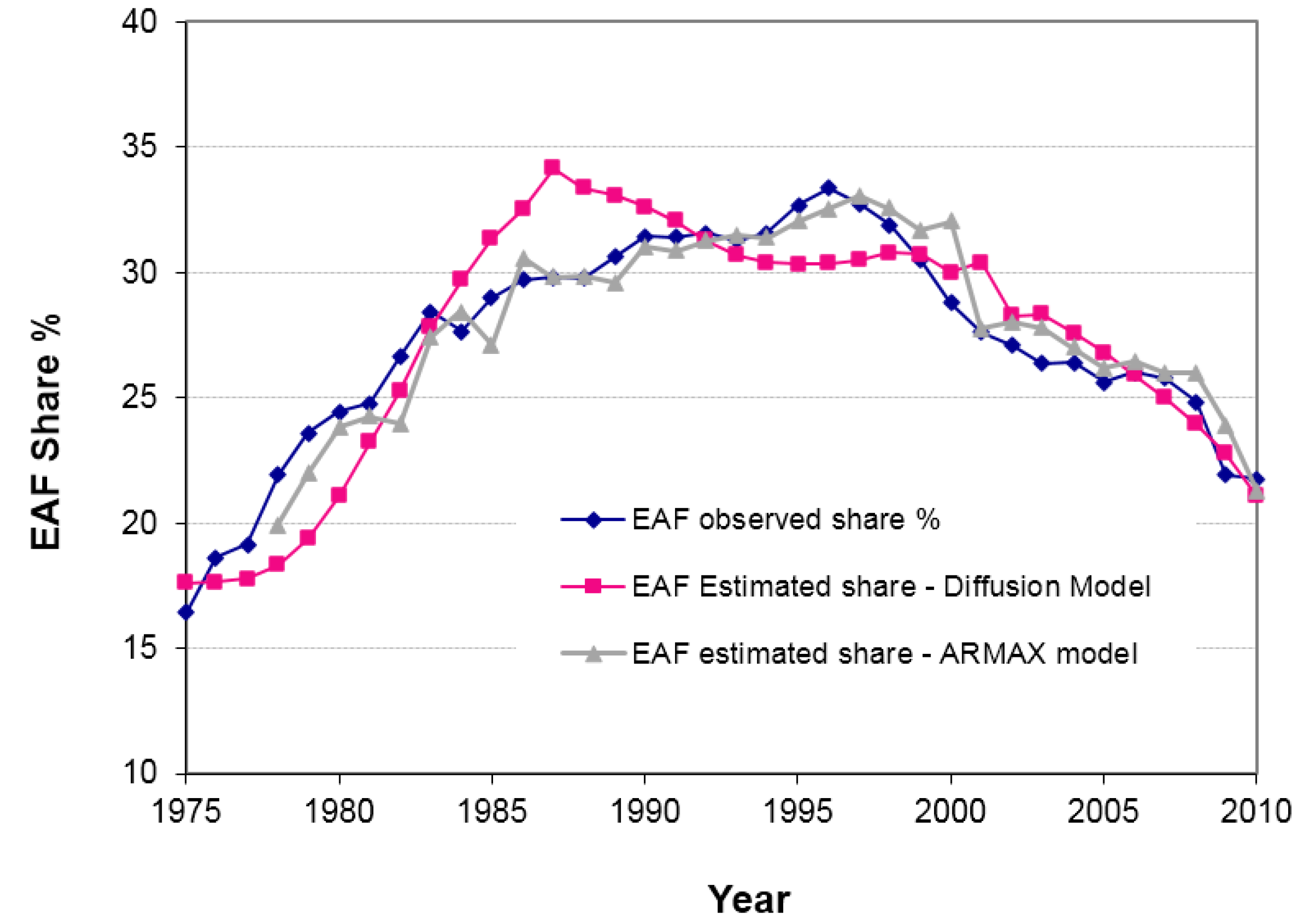
3. Application to the Case of the Diffusion of an Energy Efficient Technology: The Diffusion of Electric Arc Furnaces (EAF) in Japan

The diffusion of electric arc furnaces (EAF) in the steel industry has been studied quite intensively [34,35,36,37]. Moreover, Crompton [35] is also focused on the Japanese steel industry. In these references, neither relative scrap prices nor energy prices manage to explain the empirical diffusion pattern. However, as the proposed approach relies on some explanatory reasons to describe how the technologies evolve, we check in Section 3.1 the goodness of an ARMAX model that uses the prices of scrap, electricity, and steel to model EAF production in Japan. The purpose of using the ARMAX model is to define a linear combination of parameters that work, and can be used in function f(t) in (4), that is, that can be used as the driving force of the innovations in the new approach. Once we check the ability of those variables to depict the evolution of EAF, we apply in Section 3.2 the approach to the diffusion processes discussed in Section 2 to the diffusion of EAF technology in Japan. Moreover, it is the goodness of the ARMAX model presented in Section 3.1 (or the ability of the explanatory variables to play the role of the main driver of the innovation process) that lead us to select the diffusion of the EAF production in Japan to present the approach followed in this paper.
The information up to 1997 in the second and third columns of Table 1 comes from [38]. This information has been completed up to 2010. The sixth column lists the share of the EAF production observed in Japan. The seventh and eighth columns contain the shares estimated using the ARMAX model (introduced in Section 3.1) and when using the approach proposed in this paper to model the diffusion of innovations (Section 3.2). The scrap price shown in Table 1 was taken from [39]; the steel price and the exchange rate (yen/euro) from [40] and [41], respectively. The Japanese steel production figures and the share of Japanese EAF steel production are drawn from [42], the electricity price from [43]. Columns 3 to 5 list the prices of scrap, electricity, and steel, respectively, in constant 2005 Euros.
Before introducing the ARMAX model in Section 3.1, we first discuss some of the factors affecting the competitiveness of the Japanese steel production, some of which can be read directly from Table 1.
During the first years included in Table 1, the average cost of the scrap consumed by the Japanese industry accounted for around 25% of the price of the product, whereas during recent years this share was around 50%, reaching a maximum of 66% in 2011. Although minor, the historical ups and downs of the electricity price have also affected the competitiveness of the EAF technology in Japan, and although the electricity cost represented around 5% of the final price in 2011, in 2000 this percentage was up to 25%. Moya et al. [44] shows that the current lack of competitiveness of the Japanese EAF production, the worst performer among the countries analysed in that reference, is mainly due to the higher contribution to the steel production cost from the scrap in Japan than in the rest of countries.
From 1998 to 2008, production using the traditional route in Japan increased from 63.7 Mt to 89.3 Mt at the expense of production from the innovative EAF which stagnated at around 29 Mt (29.8 Mt in 1998 and 29.4 Mt in 2008).
Additionally, to put the analysis in the right context, we have to add that, historically, around one third of Japan’s steel production is exported and provide some notes about the different steel products and their different added value.
According to its final shape and use, steel can be classified into two big groups: flat and long products. The flat products, produced mainly by the integrated route, provide the highest added value to the steel, whereas the long products, produced mainly in the recycling route, are in the lower range of added value. In any case, the historically-clear difference between the production route and long or flat products is waning out, improving the competitiveness of the EAF technology. Nowadays 100% of long products and 70–80% of flat products can be made with scrap [45].
The recent growth of the Chinese steel production capacity in later years (doubled from 2005–2011 in which the production rose from 355 Mt to 701 Mt), combined with their overcapacity (200 Mt in 2013) and lower production costs for the long products coming from the recycling route, is a real threat to Japanese EAF producers not specialised in the highest added value products. For these last products the analysis in [44] shows that the Japanese steel industry is still able to compete in production costs with its Chinese counterpart.
The trend of the penetration of EAF in Japan cannot be globally generalized. In fact, in the steel industry of the EU, the production share of the recycling route (EAF) has increased from 20% in the 1970s to around 40% today. In some countries this share is currently about 60% (United States, Turkey, Spain, Italy, and Mexico), and in other countries (Portugal, Malaysia and Luxembourg), the EAF technology has completely replaced the incumbent technology.

3.1. Adjustment of the Diffusion of EAF in Japan with an ARMAX Model

In this section, we first check whether the EAF production can be explained by an ARMAX model. The use of this kind of model (ARMAX) has not been widely investigated to forecast diffusion of technology innovations [46]. One of the reasons for this is that much of the data used describes consumption or production, rather than the percentage of installed capacity using the innovation [6]. We opt to follow this approach, on the assumption that the competitive production exploiting the innovative technology is what drives/justifies the increase of the capacity; otherwise, if production becomes uncompetitive with the incumbent technology, the main driver for the penetration ceases to operate. Indeed, after a period it becomes a strong driver to phase out the capacity already installed.
It is worth noting that the decrease in EAF production in Japan since the 1990s means that the fit of the data with an S-shape curve does not reflect that decline. In Japan, this fact cannot be explained by a decrease in overall steel production as the total steel production since the 1970s is relatively stable, varying around 104 Mt with a standard deviation of around 8 Mt.
The ARMAX model encompasses autoregressive (AR), moving-average (MA) and regression models (i) in any combination. In general terms, it can be expressed as:
h armax ( t ) = C a r max + i = 1 r R i a r max h ( t i ) + j = 1 m M j a r max e r e s i d ( t j ) + k = 1 n l = 1 o β k a r max X k ( t l ) + e r e s i d ( t )
where Carmax is the constant coefficient, Riarmax the autoregressive coefficients, Mjarmax the moving-average coefficients, and β k a r max the regression coefficients. Each k of the Xk(t) vectors denotes one of the explanatory time series.
In this particular case, the best adjustment uses three previous values of time for the autoregressive component (r = 3), ignores the moving average (m = 0) and uses two previous values (o = 2) of three (n = 3) explanatory variables (price of scrap, electricity, and steel).
The observed and estimated share of the EAF technology using the ARMAX model, columns 6 and 7 of Table 1, are represented in Figure 1. R2, measuring the fraction of the total variability explained by the model, is 0.90, and once adjusted to reflect the complexity of the model (12 parameters), the adjusted R2 is 0.85. The mean absolute percentage error (MAPE) is 3.15%. Appendix B provides the ‘R’ script used to adjust Equation (5).
This adjustment shows that the evolution of the diffusion of the EAF can be explained using an ARMAX model with three explanatory variables. This model is able to reproduce the evolution of EAF production. The fact that the ARMAX model needs up to three and two previous values of the production and explanatory values, respectively, confirms the inertia of EAF production.

3.2. Adjustment of the Diffusion Equation to the Case of EAF in Japan

The analogy with the diffusion processes of natural phenomena can be used to construct an alternative model to the traditional diffusion model. For a function to be able to explain the number of cost-effective innovations (the main drivers of the diffusion process), we use a linear combination of the explanatory variables used in the ARMAX model:
f(t) = β0 + β1 SteelPrice(t) + β2 ScrapPrice(t) + β3 ElectricityPrice(t)
The solution EAFestimated of the diffusion process (at x = L) is the result of the integral of convolution given in Equation (4) using, for f(t), Equation (6). In principle, to estimate EAFestimated we have first to adjust six parameters, β0, β1, β2, β3, L, and K. However, since the solution is invariant for the same values of L2/K, we fix the value of L and vary K. Therefore, the model requires the adjustment of five parameters that can be found by minimising the sum of squared error between the model EAFestimated and the values observed EAFobserved; in other words, finding the minimum of:
min { t = 1970 t = 2010 [ E A F o b s e r v e d ( t ) E A F e s t i m a t e d ( t ) ] 2 }
The values of EAFobserved and EAFestimated, represented in Figure 1, are shown in the sixth and eighth columns of Table 1. Although this adjustment is slightly poorer than the ARMAX model (now the adjusted R2 = 0.76 and MAPE = 6.41%), it incorporates the average effect of the barriers and main drivers of production (Equation (6)) to explain the penetration of the energy efficient technology (EAF). It manages to do so with only five parameters, instead of the 12 used by the ARMAX model.
Appendix A includes all the code used to solve the minimisation problem (Equation (7)) and produce the results provided in column eight of Table 1.

4. Discussion

Although the ARMAX model presented in Section 3.1 describes the EAF production well, it does not include any term to describe how the impetus for new investments in EAF can be tempered. In Japan’s industrial landscape this can be due to many different factors (that effect is not described by the variables that explain the motivation for adopting EAF production; the prices of steel, scrap, and electricity). It is the function response, and in particular, the term (L2/K), that describes how the barriers present in the social medium temper the impetus for new investments. As this analysis is limited to the steel production of just one country we cannot draw any further conclusions about the relationship of conductivity to innovations and the traits of the country. In any case, as the term L is related to the size of the medium in which the diffusion takes place, its square power in the term L2/K means that policy measures designed to decrease its value can prove more beneficial than those designed to increase the conductivity of the media to innovation. However, as this last term K is inversely proportional to barriers, a sensitivity analysis of its variation among countries can shed light on measures to increase its value (and, therefore, decrease the effect of barriers).
When solving the diffusion equation, we can deal with the invariability of the solutions to the same values of L2/K keeping either K or L constant and estimating the value of the other term that makes the solution of the equation similar to the observed data. Keeping the K constant is similar to the reasoning in [47] to roughly explain historical diffusion of technologies worldwide. This thesis can be summarised by saying that the creativity, or susceptibility to innovations, of different human groups are quite similar, and that the reason why some societies were still in the Stone Age during part of the last century was due to the dimensions of the geographical context/size of their medium.
The gap between current technologies and cost-effective innovations that could be implemented but are not, is widely known as the ‘energy-efficiency gap’ [48,49]. To close that gap is one of the concerns of policy makers. The diffusion of technologies that are cost-effective should be a private-sector endeavour [50]; however, there is a clear need for the public sector to mitigate possible barriers that prevent the full deployment of these technologies.
The technology-push measures adopted by some public authorities (through policies that stimulate research and development) may decrease the investment costs of new technologies. Following the model proposed in this paper, the effect would be to increase the main driver h of technology diffusion; where h is the function that defines the push or main driver to the innovation process. Many of the demand-pull instruments that make innovations more attractive, such as emission taxes, adoption subsidies, or direct public-sector investments, can increase the incentives for using new cleaner technologies and lower the costs, thanks to a learning-by-doing effect. Again, the effect of these measures may take the form of an increase in h. Public intervention can also support the alleviation of some of the barriers, for example by means of demonstration projects that can create the research environment and networking that ease the diffusion of innovations. This kind of public intervention can be incorporated in the modelling of the diffusion process by means of the conductivity of the medium (inverse of the resistance of the medium to innovation).
The approach proposed in this paper describes the way in which the diffusion of technology is spread over society. This model explicitly incorporates a conductivity of the medium inversely proportional to the effect of barriers that define the resistance to innovation. Hitherto, state-of-the-art, bottom-up models studying energy efficiency in industry have described the current technological stock and the technology options in detail, though describing the adoption of innovations by the use of an adjusted discount rate that makes the model resemble the rate of historical diffusion [49,51]. There are some other models that use an exogenous technology diffusion rate that summarises the overall effect of the drivers and barriers. This paper shows that not only the effect of barriers but also the dimension of the medium in which the diffusion takes place can be incorporated into energy-system models, provided that the main drivers of dissemination of that technology are known.

5. Conclusions

This paper presents the modelling of the technology diffusion process using an analogy to the diffusion of natural processes. The mathematical resolution of the diffusion equation incorporates some properties that average the ease (or its inverse, the resistance) that the medium offers to the diffusion process. This is achieved at the expense of the conceptual abstraction needed to replace the medium in which the diffusion of natural processes takes place by a social medium. The approach has been applied to the currently ongoing process of the diffusion of electric arc furnaces in Japan. Despite the abstraction necessary to define the medium in which the diffusion occurs, the mathematical formulation is conceptually straightforward. However, its resolution can be cumbersome. Both factors, the abstraction needed and the cumbersome resolution of the equations, may explain why this approach has not been previously proposed. Moreover, it offers many new paths to understanding the role of the conductivity (or its inverse, the resistance) of the medium to the diffusion of innovations. The research needed to understand the term (L2/K) for different technologies and contexts (social media) can lead to an improvement in how the effect of barriers and support measures are incorporated in energy-systems models, and support, as the overall objective, the understanding of more effective ways in which policy-makers can support and encourage the innovation process.

Acknowledgments

The author would like to thank the three anonymous reviewers for their valuable comments on an earlier draft of this paper, and Gillian Harrison for editing the English of this paper.

Conflicts of Interest

The author declares no conflict of interest.

Abbreviations

The following abbreviations are used in this manuscript:
EAFelectric arc furnace
ARMAXautoregressive moving-average and regression models
MAPEmean absolute percentage error

Appendix A

This appendix contains the Mathematica code programed to solve the minimization (7). The code contains comments that allows the reader to identify the Expressions (4), (6), and (7).
The file ‘JAPAN_Mathematica_data.txt’ is an ascii file with five columns (without header) and 38 rows. To prepare that file the reader has to copy and paste the numerical content of columns 3, 4, 5, and 6 of Table 1 to an ascii file called ‘JAPAN_Mathemaica_data.txt’. As additional step, when running the Mathematica code, the reader has to make accessible this file (see the first line of the code).
To run the following Mathematica code the reader has to incorporate the following code to a mathematica file ‘*.nb’ and run it.
  • SetDirectory["working directory"]
  • datos = ReadList["JAPAN_Mathematica_data.txt", Number, RecordLists -> True];
  • {year, steelPrice, scrapPrice, eleJP, perJP} = Transpose[datos];
  • (*Expression (6), function driver of innovations*)
  • Tdriver2[Diff_, L_, B0_, B1_, B2_, B3_, ele_] := Join[
  • Table[{i, 0}, {i, 0, 1973}], Transpose[{Table[i, {i, 1974, 2011}],
  • Apply[Plus, Transpose[{Table[B0, {i, 1974, 2011}], B1steelPrice,B2scrapPrice, B3ele}], 1]}]];
  • funcion[Diff_, L_, B0_, B1_, B2_, B3_, ele_] := Interpolation[Tdriver2[Diff, L, B0, B1, B2, B3 , ele]];
  • (*Expression (4), convolution *)
  • Convo[Diff_?NumericQ, L_?NumericQ, B0_?NumericQ, B1_?NumericQ,
  • B2_?NumericQ, B3_?NumericQ, tt_?NumericQ, per_, ele_] := (
  • percen = Transpose[{Table[i, {i, 1974, 2011, 1}], per}];
  • Min[Hold[(Plus @@ {percen[[1, 2]], percen[[2, 2]], percen[[3, 2]]})/3 +
  • NIntegrate[(funcion[Diff, L, B0, B1, B2, B3, ele][tt - t]) (
  •  L E^(-(L^2/(4 Diff t))))/(2 Sqrt[[Pi] Diff] t^(3/2)), {t, 0, tt},
  • WorkingPrecision -> 4, MinRecursion -> 5, AccuracyGoal -> 2]], 100]);
Plotconvo[Diff_?NumericQ, B0_?NumericQ, B1_?NumericQ, B2_?NumericQ, B3_?NumericQ, per_, ele_] := Table[Convo[Diff, 1, B0, B1, B2, B3, t, per, ele], {t, 1974, 2011}];
  • SSEE[{{x_, y_} /; (Release[x] - y)^2 < 10000, Resto___}] := (Release[x] - y)^2 + SSEE[{Resto}]
  • SSEE[{{x_, y_} /; (Release[x] - y)^2 >= 10000, Resto___}] := 10^10
  • SSEE[{}] := 0
  • Ajuste2[Diff_?NumericQ, B0_?NumericQ, B1_?NumericQ, B2_?NumericQ,
  • B3_?NumericQ, per_, ele_] :=
  • SSEE[Transpose[{Release[Plotconvo[Diff, B0, B1, B2, B3, per, ele]], per}]]
  • Ajuste2[{Diff_, B0_, B1_, B2_, B3_}, {per___}, {ele___}] := Ajuste2[Diff, B0, B1, B2, B3, {per}, {ele}]
  • Resul[Diff_?NumericQ, B0_?NumericQ, B1_?NumericQ, B2_?NumericQ, B3_?NumericQ, per_, ele_] :=
  •  Transpose[{Table[i, {i, 1974, 2011}], Release[Plotconvo[Diff, B0, B1, B2, B3, per, ele]]}];
  • Resul[{Diff_, B0_, B1_, B2_, B3_}, {per___}, {ele___}] := Resul[Diff, B0, B1, B2, B3, {per}, {ele}]
  • Dibuja4[Diff_, B0_, B1_, B2_, B3_, per_, ele_] :=
  • (Show[ ListPlot[Transpose[{Table[i, {i, 1974, 2011}], per}],
  •  PlotStyle -> {Blue, PointSize[.02]}],
  •  ListPlot[Resul[Diff, B0, B1, B2, B3, per, ele], PlotStyle -> {Green, PointSize[.02]}] ] )
  • Dibuja4[{Diff_, B0_, B1_, B2_, B3_}, {per___}, {ele___}] := Dibuja4[Diff, B0, B1, B2, B3, {per}, {ele}]
  • (*Expression (7), minimization *)
  • (*the running time of will depend on the computer*)
  • NMinimize[{Ajuste2[Diff, B0, steel, scrap, elec, perJP, eleJP], Diff > 0.0000000000001}, {Diff, B0, steel, scrap, elec}, Method -> "DifferentialEvolution"]
(* Using the values of β0, β1, β2, β3 and K solution of the previous minimization, the following function Dibuja4 draws Figure 1*)
Dibuja4[.0144956, .016119, 0.833622, -2.17326, -.31262, perJP, eleJP]
  • (*the following line produces the estimated share of EAF in Japan, column 8 of Table 1 *)
  • estJP = Transpose[Resul[.0144956, .016119, 0.833622, -2.17326, -.31262, perJP,eleJP]][[2]]

Appendix B

This appendix contains the ‘R‘ script used to adjust the ARMAX model, Equation (5). This code uses the library ‘dse‘ [52], and an acsii file ‘EAF_japan.csv‘ that the reader can prepare with the input values of Table 1.
  • # load library "dse"
  • library("dse")
  • # the file"EAF_japan.csv" has 38 rows (one row per year between 1974 and 2011)
  • # and 4 columns:
  • # column 1 has the EAF production (Mt) (is the product of column 2 and 6 of Table 1)
  • # columns 2, 3 and 4 of the file correspond with columns 3, 4 and 5 of Table 1)
  • datos<-read.csv("EAF_japan.csv",header=T, sep = ";", dec=".",as.is=TRUE)
  • # create a time series taking differences
  • # for the explanatory variables we take differences of their log
  • tsdatos<-TSdata(input=apply(log(datos[,2:4]),2,diff),output=diff(datos[,1]))
  • # name the explanatory variables and the output
  • seriesNamesInput(tsdatos)<-c("scrap_price","elec_price","steel_price")
  • seriesNamesOutput(tsdatos)<-"EAF_production"
  • # estimate the ARMAX model with three lags
  • model1<-estVARXls(tsdatos,max.lag=3)
  • # coeficients of the ARMAX model
  • model1

References

  1. Barreto, L.; Kemp, R. Inclusion of technology diffusion in energy-systems models: Some gaps and needs. J. Clean. Prod. 2008, 16, 95–101. [Google Scholar] [CrossRef]
  2. Griliches, Z. Hybrid corn: An exploration in the economics of technological change. Econometrica 1957, 25, 501–522. [Google Scholar] [CrossRef]
  3. Rogers, E.M. Diffusion of Innovations, 5th ed.; The Free Press: New York, NY, USA, 2003. [Google Scholar]
  4. Sarkar, J. Technological diffusion: Alternative theories and historical evidence. J. Econ. Surv. 1998, 12, 131–176. [Google Scholar] [CrossRef]
  5. Geroski, P.A. Models of technology diffusion. Res. Policy 2000, 29, 603–625. [Google Scholar] [CrossRef]
  6. Meade, N.; Islam, T. Modelling and forecasting the diffusion of innovation—A 25-year review. Int. J. Forecast. 2006, 22, 519–545. [Google Scholar] [CrossRef]
  7. Chandrasekaran, D.; Tellis, G.J. A Critical Review of Marketing Research on Diffusion of New Products. In Review of Marketing Research; Malhotra, N.K., Ed.; Emerald Group Publishing Limited: Bingley, UK, 2007; Volume 3, pp. 39–80. [Google Scholar]
  8. Fisher, J.C.; Pry, R.H. A simple subtitution model of technological change. Technol. Forecast. Soc. Chang. 1971, 3, 75–88. [Google Scholar] [CrossRef]
  9. Mansfield, E. Technical change and the rate of imitation. Econometrica 1961, 29, 741–765. [Google Scholar] [CrossRef]
  10. Bass, F. A new product growth model for consumer durables. Manage Sci. 1969, 15, 215–227. [Google Scholar] [CrossRef]
  11. Mulder, P.; De Groot, H.L.F.; Hofkes, M.W. Economic growth and technological change: A comparison of insights from a neo-classical and an evolutionary perspective. Technol. Forecast. Soc. Chang. 2001, 68, 151–171. [Google Scholar] [CrossRef]
  12. Romer, P.M. Increasing returns and long-run growth. J. Polit. Econ. 1986, 94, 1002–1037. [Google Scholar] [CrossRef]
  13. Lucas, R.E. On the mechanics of economic development. J. Monet. Econ. 1988, 22, 3–42. [Google Scholar] [CrossRef]
  14. David, P.A. A Contribution to the Theory of Diffusion; Centre for Research in Economic Growth Research Memorandum, Stanford University: Standford, CA, USA, 1969. [Google Scholar]
  15. Montalvo, C.; Kemp, R. Cleaner technology diffusion: Case studies, modeling and policy. J. Clean. Prod. 2008, 16, S1–S6. [Google Scholar] [CrossRef]
  16. Fernandez, V.P. Forecasting home appliance sales: Incorporating adoption and replacement. J. Int. Consum. Mark. 1999, 12, 39–61. [Google Scholar] [CrossRef]
  17. Jain, D.C.; Rao, R.C. Effect of Price on the Demand for Consumer Durables: Modeling, Estimation, and Findings. J. Bus. Econ. Stat. 1990, 8, 163–170. [Google Scholar]
  18. Hlavinka, A.N.; Mjelde, J.W.; Dharmasena, S.; Holland, C. Forecasting the adoption of residential ductless heat pumps. Energy Econ. 2016, 54, 60–67. [Google Scholar] [CrossRef]
  19. Shinohara, K. Space-time innovation diffusion based on physical analogy. Appl. Math. Sci. 2012, 6, 2527–2558. [Google Scholar]
  20. Suriñach, J.; Autant-Bernard, C.; Manca, F.; Massard, N.; Moreno, R. The Diffusion/Adoption of Innovation in the Internal Market; Economic Papers No. 384; Dirctorate-General Economic and Finantial Affairs, European Commission: Brussels, Belgium, 2009. [Google Scholar]
  21. Hall, B.; Khan, B. Adoption of New Technology. NBER Working paper series. Working paper 9730. 2003. Available online: http://www.nber.org/papers/w9730.pdf (accessed on 16 January 2014).
  22. European Commission. Communication from the Commission to the European Parliament, the Council, the European Economic and Social Committee, the Committe of the Regions and the European Investment Bank; COM(2015) 572; State of the Energy Union: Brussels, Belgium, 2015. [Google Scholar]
  23. Fleiter, T.; Plötz, P. Diffusion of energy efficient technologies. Encycl. Energy Nat. Resour. Environ. Econ. 2013, 1, 63–73. [Google Scholar]
  24. Jaffe, A.B.; Stavins, R.N. The energy-efficiency gap What does it mean? Energy Policy 1994, 22, 804–810. [Google Scholar] [CrossRef]
  25. Hirst, E.; Brown, M. Closing the efficiency gap: barriers to the efficient use of energy. Resour. Conserv. Recycl. 1990, 3, 267–281. [Google Scholar] [CrossRef]
  26. Domenico, P.A.; Schwartz, F.W. Physical and Chemical Hydrogeology, 2nd ed.; Wiley: New York, NY, USA, 1998. [Google Scholar]
  27. Freeze, R.A. Henry Darcy and the fountains of Dijon. Ground Water 1994, 32, 23–30. [Google Scholar] [CrossRef]
  28. Okazaki, T.; Yamaguchi, M. Accelerating the transfer and diffusion of energy saving technologies steel sector experience-lessons learned. Energy Policy 2011, 39, 1296–1304. [Google Scholar] [CrossRef]
  29. Bear, J. Dynamics of Fluids in Porous Media (Dover Civil and Mechanical Engineering); Dover Publications: New York, NY, USA, 1988. [Google Scholar]
  30. Moore, M.C.; Arent, D.J.; Norland, D. R&D advancement, technology diffusion, and impact on evaluation of public R&D. Energy Policy 2007, 35, 1464–1473. [Google Scholar]
  31. Crank, J. The Mathematics of Diffusion, 2nd ed.; Claredon Press: Oxford, UK, 1975. [Google Scholar]
  32. Smith, G.D. Numerical Solution of Partial Differential Equations: Finate Difference Methods (Oxford Applied Mathematics and Computing Science Series), 3rd ed.; Oxford University Press: New York, NY, USA, 1985. [Google Scholar]
  33. Ames, W.F. Numerical Methods for Partial Differential Equations. Computer Science and Scientific Computing, 3rd ed.; Academic Press Limited: San Diego, CA, USA, 1992. [Google Scholar]
  34. Nill, J. Diffusion as time-dependent result of technological evolution, competition, and policies: The case of cleaner iron and steel technologies. J. Clean. Prod. 2008, 16, 58–66. [Google Scholar] [CrossRef]
  35. Crompton, P. The diffusion of new steelmaking technology. Resour. Policy 2001, 27, 87–95. [Google Scholar] [CrossRef]
  36. Labson, B.S.; Gooday, P. Factors influencing the diffusion of electric arc furnace steelmaking technology. Appl. Econ. 1994, 26, 917–925. [Google Scholar] [CrossRef]
  37. Reppelin-Hill, V. Trade and environment: An empirical analysis of the technology effect in the steel industry. J. Environ. Econ. Manag. 1999, 38, 283–301. [Google Scholar] [CrossRef]
  38. Crompton, P. Forecasting steel consumption in South–East Asia. Resour. Policy 1999, 25, 111–123. [Google Scholar] [CrossRef]
  39. USGS. USGS Minerals Information: Iron and Steel Scrap. 2012. Available online: http://minerals.usgs.gov/minerals/pubs/commodity/iron_&_steel_scrap/ (accessed on 18 October 2013). [Google Scholar]
  40. The World Bank. Global Economic Monitor (GEM) Commodities Database. 2012. Available online: http://databank.worldbank.org/data/databases.aspx (accessed on 3 October 2013).
  41. Fxtop company. Historical-exchange-rates. 2016. Available online: http://fxtop.com/en/historical-exchange-rates.php?A=1&C1=EUR&C2=JPY&YA=1&DD1=01&MM1=01&YYYY1=1974&B=1&P=&I=1&DD2=01&MM2=01&YYYY2=2012&btnOK=Go%21 (accessed on 19 March 2016).
  42. Worldsteel. Steel statistical yearbook (several volumes). 2013. Available online: http://www.worldsteel.org/ (accessed on 25 September 2013).
  43. International Energy Agency (IEA). Electricity Information (several volumes). 2013. Available online: http://www.oecd-ilibrary.org/energy/electricity-information-2001_electricity-2001-en (accessed on 12 October 2013).
  44. Moya, J.A.; Boulamanti, A. Production Costs from Energy-intensive Industries in the EU and Third Countries; EUR-Scientific and Technical Research Reports; Publications Office of the European Union: Luxembourg City, Luxembourg, 2016. [Google Scholar] [CrossRef]
  45. Genet, M. Impacts of the energy market developments on the steel industry. In Presented at the 74th session of the OECD Steel Committee [Online], Paris, France, 1–2 July 2013; OECD Web site. http://www.oecd.org/sti/ind/Item%209.%20Laplace%20-%20Steel%20Energy.pdf (accessed on 25 November 2013).
  46. Christodoulos, C.; Michalakelis, C.; Varoutas, D. Forecasting with limited data: Combining ARIMA and diffusion models. Technol. Forecast. Soc. Chang. 2010, 77, 558–565. [Google Scholar] [CrossRef]
  47. Diamond, J. Guns, Germs, and Steel: The Fates of Human Societies, 1st ed.; W.W. Norton: New York, NY, USA, 1997. [Google Scholar]
  48. Bunse, K.; Vodicka, M.; Schönsleben, P.; Brülhart, M.; Ernst, F.O. Integrating energy efficiency performance in production management—Gap analysis between industrial needs and scientific literature. J. Clean. Prod. 2011, 19, 667–679. [Google Scholar] [CrossRef]
  49. Cooremans, C. The role of formal capital budgeting analysis in corporate investment decision making a literature review. In Proceeding of eceee 2009 Summer Study Act! Innovate! Deliver! Reducing energy demand sustainability, La Colle sur Loup, France, 1–6 June 2009.
  50. Halsnæs, K.; Shukla, P.; Ahuja, D.; Akumu, G.; Beale, R.; Edmonds, J.; Gollier, C.; Grübler, A.; Ha Duong, M.; Markandya, A.; et al. Framing issues. In Climate Change 2007: Mitigation of Climate Change; Contribution of Working Group III to the Fourth Assessment Report of the Intergovernmental Panel on Climate Change, Metz, B., Davidson, O.R., Bosch, P.R., Dave, R., Meyer, L.A., Eds.; Cambridge University Press: Cambridge, UK; New York, NY, USA, 2007. [Google Scholar]
  51. Fleiter, T.; Worrell, E.; Eichhammer, W. Barriers to energy efficiency in industrial bottom-up energy demand models—A review. Renew. Sustain. Energy Rev. 2011, 15, 3099–3111. [Google Scholar] [CrossRef]
  52. Gilbert, P.D. Brief User’s Guide: Dynamic Systems Estimation distributed with the dse package. (2006 or later). Available online: http://cran.r-project.org/web/packages/dse/vignettes/Guide.pdf (accessed on 11 January 2014).
Figure 1. Historical record of Japanese EAF share and estimated shares using an ARMAX model and the diffusion model presented in this paper.
Energies 09 00471 g001
Table 1. Parameters explaining the share of steel production using EAF in Japan, observed share (column 6) and its estimations (columns 7 and 8).
Column 1Column 2Column 3Column 4Column 5Column 6Column 7Column 8
YearTotal Steel ProductionScrap PriceElectricity PriceSteel PriceEAF ObservedEAF EstimatedEAF Estimated Share
shareshare ARMAX ModelDiffusion Model. Section 3.2
MtEUR/tEUR/MWhEUR/t%%%
1974117.1272.8143.6850.317.8 17.6
1975102.3167.2129.0778.216.4 17.6
1976102.3171.9130.5737.718.6 17.6
1977107.4132.4107.6694.619.1 17.8
1978102.4149.372.0649.021.919.918.3
1979111.7176.078.0599.523.622.019.4
1980111.4151.585.8550.624.523.821.1
1981101.7140.1122.8477.024.824.323.2
198299.588.9181.8347.626.624.025.3
198397.299.3215.1306.828.427.527.8
1984105.6114.5269.1310.727.728.529.7
1985105.389.0308.6290.92927.131.4
198698.392.3154.2277.729.730.632.5
198798.5103.6106.1250.329.829.834.2
1988105.7127.586.7312.829.729.933.4
1989107.9121.691.8391.930.629.633.1
1990110.3117.375.7402.831.431.032.6
1991109.698.573.7393.031.430.832.0
199298.189.067.5321.031.631.231.3
199399.6114.567.4356.531.231.530.7
199498.3127.163.4322.831.631.430.4
1995101.6132.455.0374.332.332.030.3
199698.8126.268.4346.833.332.530.4
1997104.5124.091.0307.932.833.030.5
199893.5101.289.8241.231.932.630.8
199999.586.896.0216.231.931.730.7
2000106.486.7123.0220.528.832.130.0
2001102.966.2129.3195.527.627.830.4
2002107.776.5112.9177.527.128.028.3
2003110.5101.478.4226.626.427.828.4
2004112.7170.164.3355.726.427.027.6
2005110.5151.962.8340.126.426.226.8
2006116.2166.963.6346.02626.425.9
2007120.2189.254.3396.225.826.025.0
2008118.7260.050.1566.424.826.023.9
200987.5153.857.6359.421.923.922.8
2010109.6233.059.8410.921.821.321.0
2011107.6280.958.3451.423.122.420.2

