Article

Part-Load Performance Prediction and Operation Strategy Design of Organic Rankine Cycles with a Medium Cycle Used for Recovering Waste Heat from Gaseous Fuel Engines

State Key Laboratory of Engines, Tianjin University, Tianjin 300072, China
*
Author to whom correspondence should be addressed.
Energies 2016, 9(7), 527; https://doi.org/10.3390/en9070527
Submission received: 15 May 2016 / Revised: 21 June 2016 / Accepted: 28 June 2016 / Published: 11 July 2016
(This article belongs to the Special Issue Organic Rankine Cycle (ORC))

Abstract

:
The Organic Rankine Cycle (ORC) is regarded as a suitable way to recover waste heat from gaseous fuel internal combustion engines. As waste heat recovery systems (WHRS) have always been designed based on rated working conditions, while engines often work under part-load conditions, it is quite significant to analyze the part-load performance and corresponding operation strategy of ORC systems. This paper presents a dynamic model of ORC with a medium cycle used for a large gaseous fuel engine and analyzes the effect of adjustable parameters on the system performance, giving effective control directions under various conditions. The results indicate that the intermediary fluid mass flow rate has nearly no effect on the output power and thermal efficiency of the ORC, while the mass flow rate of working fluid has a great effect on them. In order to get a better system performance under different working conditions, the system should be operated with the working fluid mass flow rate as large as possible, but with a slight degree of superheating. Then, with the control of constant superheat degree at the end of the heating process, the performance of the combined system that consists of ORC and the engine at steady state under seven typical working conditions is also analyzed. The results indicate that the energy-saving effect of WHRS becomes worse and worse as the working condition decreases. Especially at 40% working condition the WHRS nearly has no energy-saving effect anymore.

1. Introduction

The Organic Rankine Cycle (ORC) is regarded as a suitable way to recover exhaust waste heat from gaseous fuel internal combustion engines (ICEs) [1]. ORC is always designed for the rated working conditions, but needs to be operated under various working conditions as the gaseous fuel engines often work at part-load. In practice, under the different working conditions of ICEs, the exhaust gas temperature of light-duty engines varies from 500 to 900 °C and that of heavy-duty engines is in the range of 400 to 650 °C [2,3]. The investigation conducted by Chammas and Clodic [4] has shown that the available exhaust gas energy varies greatly depending on engine conditions for a typical light duty engine. A similar conclusion was obtained by Ringler [5] and Teng [6] based on a medium duty engine and typical truck diesel engine, respectively. In fact, exhaust gas flow rate and temperature variations lead the evaporator, even though properly designed, to severe conditions which make the waste heat recovery impossible [7]. The varying engine working conditions should be taken into consideration when an ORC system is designed and operated as a waste heat recovery system (WHRS) [3]. Therefore, the part-load performance prediction and operation strategy design are meaningful to make the ORC system operate efficiently and safely.
The part-load performance of an ORC system can be profitably predicted by off-design static models or dynamic models. Quoilin [8] presented an off-design static ORC model by interconnecting different sub-models including some heat exchanger models, a volumetric pump model and a scroll expander model. With the validation by experimental data, the model was finally used to investigate potential improvements of the ORC system. Yu et al. [9] used the Aspen software to establish an off-design static model of an ORC system used for a diesel engine with a power output of 240 kW which consisted of heat exchangers and expander sub-models. The static performance of the ORC under five typical engine working conditions was analyzed by the model. Manente et al. [10] also built an off-design static model of an existing 30 MW ORC plant by Aspen to calculate the values of the operating parameters that maximize the power output from an available geothermal resource.
The ORC models mentioned above are all static model which can effectively predict the steady performance of ORC systems under different working conditions, but useless to analyze the dynamic variation process and design control strategies. The dynamic model of ORC is an effective way of part-load performance prediction and control design [11,12,13]. In most researches [11,12,13,14,15,16,17,18,19,20,21,22,23,24,25,26,27], dynamic models of the main components are built first and then system model is created by appropriately combining each of the component models according to their interrelationships. Because pump and expander dynamics are very fast compared to the heat exchangers, their models are usually replaced by static models. For establishing dynamic models of the evaporator and condenser, the discretization method [14,15,16] or MB (moving boundary) method [17,18,19,20,21,22,23,24,25,26,27,28,29] are the most popular and effective approaches. Wei et al. [14] proposed two alternative approaches for a dynamic ORC model based on MB and discretization techniques, respectively. Compared to experimental data, simulation results evidenced that both models have good accuracy, but the model based on the MB method needs much less computing resources. For other research using the discretization method in ORCs readers can refer to [15,16]. However, the MB method is used much more often [17,18,19,20,21,22,23,24,25,26,27,28,29], and the MB method has been proven to be accurate enough in comparison with the experimental data [17,18,19].
The ORC dynamic model can predict part-load performance. Manente et al. [12] presented a detailed dynamic model of an ORC system to calculate the system performance under part-load conditions and find the optimal operating parameters that maximize the electricity production in response to working condition changes. The authors suggested the model can be conveniently applied to both optimization of existing plants and design of new plant configurations. Other studies [13,20] also built an ORC dynamic model as WHRS for an internal combustion engine to analyze the system performance under part-load working conditions.
Another important application of the dynamic model of an ORC by the MB approach is control design. If the ORC is used for waste heat recovery of ICEs, a current challenge is how to operate them with heat sources that are often unsteady or transient. Therefore, the control design of ORC is very important. Zhang et al. [21,22,23] applied control strategies based on linear ORC models, validated on one operating point. Benato et al. [24] used a PI (proportional integral) controller in their dynamic ORC model and the results indicated the effectiveness of the proposed control strategy. Quoilin et al. [15] proposed three control strategies with PI controllers and it was found that a model predictive control strategy based on the steady-state optimization of the cycle under various conditions is the best one. The research of Luong et al. [25] showed the benefits of multi-input multi-output LQI (Linear Quadratic Integral) control over single-input single-output PI control for the nonlinear ORC in the presence of automotive transient disturbances.
In all the dynamic ORC system models mentioned above, the organic working fluids are directly heated by the exhaust gas whose temperature is usually higher than 500 °C in evaporator. However, the decomposition temperatures of frequently-used working fluids like R245fa, R123 are usually relatively low, so it may cause local overheating and decomposition problems. In this case, a medium cycle (MC) is needed to lower the exhaust temperature first, ensuring the safety of the working fluid [26]. Besides, the MC has a thermal storage function, so it can improve the stability of an ORC system when the waste heat source changes [27]. Also for the thermal storage function, the MC can turn all step changes to ramp changes, which makes the control system have better performance and robustness. Vaja [28] displayed the importance of an intermediary fluid to transfer the heat from engine exhaust to the ORC. This is not only for safety reasons, but also to stabilize the operation of the ORC system under transient operational conditions. Gewald [26] applied an ORC with thermal-oil cycle to recover the waste heat of several large stationary engines. With the thermal-oil cycle, the waste heat of different engines can conveniently be combined into one ORC system. Moreover, for other researches that used the MC readers can refer to [29,30,31].
According to the literature reviews, there are very few studies focused on part-load performance prediction and operation strategy design of ORC-MC systems, which are significant for actual WHRS of engines. In this paper a dynamic model of an ORC-MC system using water as intermediary fluid for exhaust waste heat recovery of a large gaseous fuel engine is established. Using this model, the effect of adjustable parameters on the system performance and effective operation strategy under part-load conditions are analyzed. Then, with the control of constant superheating degree at the end of heating process, the system performance at steady state under seven typical working conditions is also analyzed.

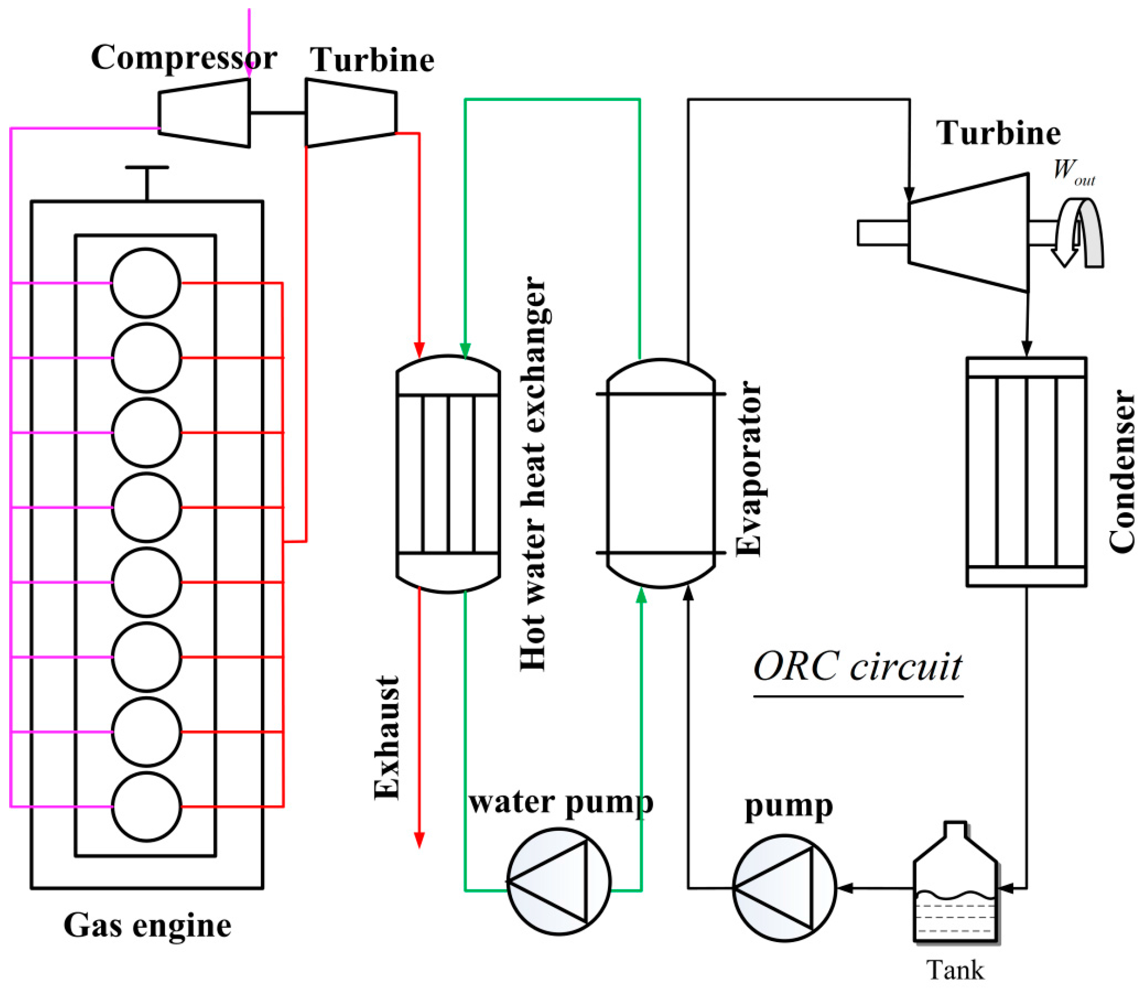
2. System Description

2.1. Gaseous Fuel Engine

The studied gaseous fuel internal combustion engine in the paper is a stationary electric generating plant of 1000 kW rated power that is designed and produced in a Chinese manufacturer. The exhaust is the heat source of the WHRS. As a power plant uses the engine, its speed is constant (600 rpm) while its load varies under different conditions. Heat balance experiments have been conducted on the gaseous fuel engine. Seven typical conditions of the engine are picked out in Table 1.
It can be seen from Table 1 that the exhaust temperature before the turbo charger is quite high. Therefore, it is very meaningful to recover the exhaust waste heat of gaseous fuel engines. Assuming that the fuel burns completely, the composition of the exhaust can be calculated according to the actual volume ratio of air and gaseous fuel: N2 = 73.4%, CO2 = 7.11%, H2O = 14.22% (gas), O2 = 5.27%. Then the specific heat capacity, enthalpy and other thermo-physical properties can be known.

2.2. ORC-MC System

The selection of the organic working fluid is an important preliminary issue. The selection criteria require the organic fluids to have low environmental impact (low ODP and low GWP), favourable thermodynamic properties (high enthalpy drop through the expander, favourable boiling temperature, large latent heat, good heat transfer, low viscosity and good thermal stability), high safety (low toxicity, low corrosion and non-flammability) and low cost [32]. Based on these requirements, R245fa was chosen as a working fluid that is also widely used in many studies such as [33,34,35]. As mentioned above, the decomposition temperature of R245fa is relative low, so an ORC-MC system is applied as the WHRS.
The fundamental principle of the system is simple: the exhaust heats water first and then the hot water is the heat source of the ORC system. It should be noticed that the hot water cycle is pressurized in order to avoid using a steam boiler. The working fluid is heated into high temperature and pressure vapor by hot water and then the vapor expands in a turbine or expander to generate power, decreasing the temperature and pressure. After that, the vapor is cooled into liquid form in the condenser. Finally the liquid working fluid is pumped to the preheater again and starts a new cycle. The system diagram and T-S diagram are shown in Figure 1 and Figure 2.

3. Mathematical Model

3.1. Sub-Models for the Main Components

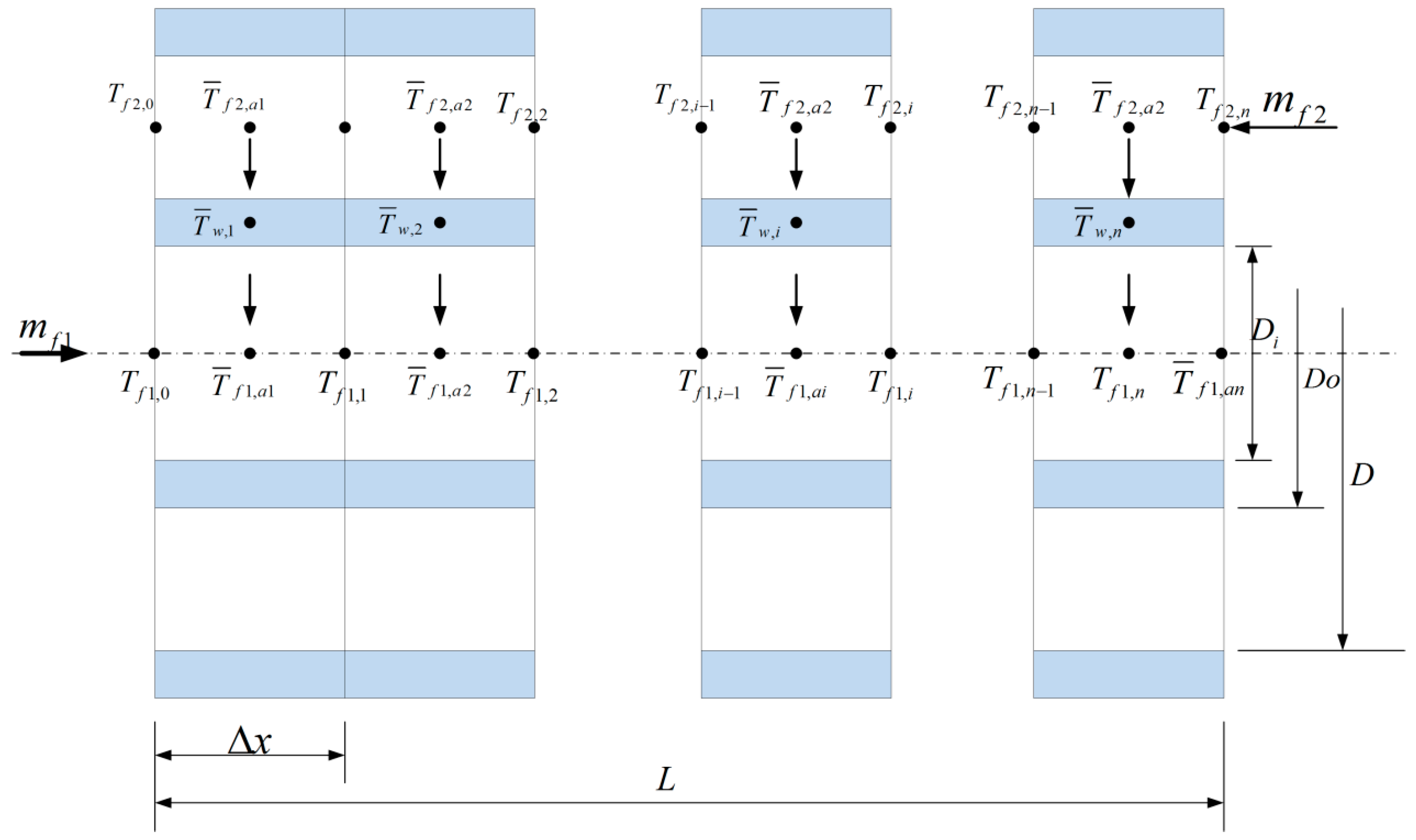
3.1.1. Hot Water Heat Exchanger

All the exchangers in this paper have been, for sake of simplicity, represented as a typical counter flow straight pipe, despite the fact it is well known that complex designs are usually adopted in order to enhance heat exchange and to reduce the overall dimensions of the system. This assumption simplifies the resulting dynamic problem to a great extent, and is commonly adopted when heat exchanger dynamic modeling is considered [28].
As there is no phase change in the water heat exchanger and the temperature of exhaust drops a lot, the discretization method is used to establish this sub-model. In the discretization model of the water heat exchanger, this straight pipe of the water heat exchanger has been split into n longitudinal lumped volumes, each of length Δx as shown in Figure 3. For each discrete volume, three nodes can be defined in the radial direction: one referring to the fluid within the internal pipe (referred to as f1); one referring to the state of the metal constituting the metal pipe (referred to as w); one referring to the state of the fluid in the annulus (f2). The discretization nodes are located at the centre of the different control cells and their state is represented by the average state of outlet and inlet of the control cell.
The assumptions introduced in the discrete model are the following:
  • The external pipe is assumed to be ideally insulated hence heat losses are neglected;
  • The exhaust finally discharges to the environment and its pressure doesn’t change a lot, so the pressure is considered constant and the head losses of water in inner pipe is also neglected. Therefore, the momentum conservation equation is not applied to the cells of fluid.
  • The hot water is considered to be incompressible and it is pressured into a constant value, while the exhaust is compressible;
  • The axial conductive heat fluxes have been neglected for the fluids and pipe wall;
  • No mass accumulation is considered for the fluids;
  • Lumped thermal capacitance is assumed for both the metal pipe.
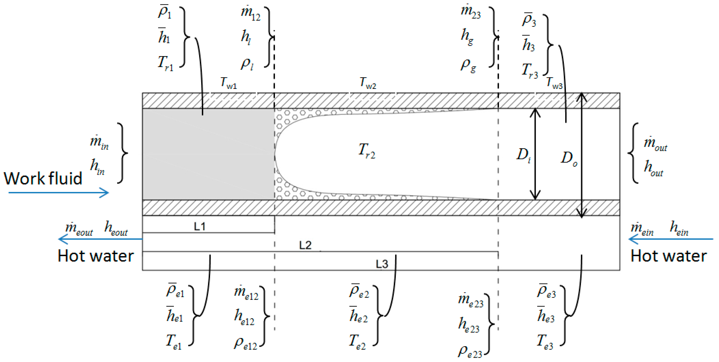
Based on the above assumptions, the following three equations can be obtained:
Hot water:
A 1 Δ x ρ ¯ f 1 , a i C ¯ p f 1 , a i d T ¯ f 1 , a i d t = α i n , i π D i Δ x ( T w , i T f 1 , a i ) + m ˙ f 1 h f 1 , i m ˙ f 1 h f 1 , i + 1
Exhaust:
A 2 Δ x ( ρ ¯ f 2 , a i C ¯ p f 2 , a i + h ¯ f 2 , a i ρ ¯ f 2 , a i h ¯ f 2 , a i ) d T ¯ f 2 , a i d t = α o u t , i π D o Δ x ( T w , i T f 2 , a i ) + m ˙ f 2 h f 2 , i + 1 m ˙ f 2 h f 2 , i
Pipe wall:
A w Δ x ρ w C p w d T ¯ w , a i d t = α o u t , i π D o Δ x ( T f 2 , a i T w , i ) + α i n , i π D i Δ x ( T f 1 , a i T w , i )
The heat transfer coefficient outside the pipe α1 can be determined by Zukauskas’ correlation [36]:
N u f = C α Re m Pr f 0.36 ( Pr f / Pr w ) 0.25
Therein, Cα and m depend on Re [36]. Subscripts f and w represent the fluid and pipe wall, respectively. There is no phase change in the tube, so the convective heat transfer coefficient for internal flow is obtained by using Sieder-Tate correlation [36]:
N u f = 0.027 Re f 0.8 Pr f 1 / 3 ( η f η w )

3.1.2. Evaporator

Because there is a phase change in the evaporator and the convective heat transfer coefficients are very different in the various phases, the moving boundary method is used to build the evaporator model. The evaporator is divided into three regions: sub-cooling region, two-phase region and superheated region. The lumped parameter method is used in each region. The idea of a moving boundary model is to dynamically track the lengths of the different regions in the heat exchanger. The modeling methods to be presented require several assumptions about the fluid flow in the heat exchangers. These assumptions are as follows [17]:
  • The heat exchanger is a long, thin, horizontal tube.
  • The working fluid and exhaust flowing through the heat exchanger tube can be modeled as a one-dimensional fluid flow.
  • Axial conduction of working fluid and exhaust is negligible.
  • Pressure drop along the heat exchanger tube due to momentum change in refrigerant and viscous friction are negligible. Thus the equation for conservation of momentum is not needed.
  • The assumption of mean void fraction is used. Void fraction is defined as the ratio of vapor volume to total volume, and has long been used to describe certain characteristics of two-phase flows.
The notations used in the moving boundary model are given in Figure 4. Other notations not appearing in the figure are α0 (the heat transfer coefficient between hot water and pipe wall), α1, α2, α3 (internal pipe heat transfer coefficient in subcooling region, two-phase region and superheated region), p (the pressure in evaporator), pe (the pressure of hot water), Ai, Ao, Aw (the cross sectional area of inner pipe, outer pipe and pipe wall).
The general differential mass balance for the three regions is:
0 L 1 ( A ρ ) t d z + 0 L 1 m ˙ z d z = 0
The general differential energy balance for the three regions is:
0 L 1 ( A ρ h A p ) t d z + 0 L 1 m ˙ h z d z = 0 L 1 α i π D i ( T w T r ) d z
A simplified differential energy balance for the wall is:
c p w ρ w A w d T w d t = α i π D i ( T r T w ) + α o π D o ( T a T w )
Equations (6)–(8) are integrated over the three regions to give the general three region lumped model for a two-phase heat exchanger. The average density of the subcooling region and superheated region is expressed as the function of the pressure and average specific enthalpy. The average specific enthalpy is arithmetic mean value of the enthalpy at inlet and outlet of subcooling region and superheated region. In two-phase region the average density and specific enthalpy can be written as:
ρ s = γ ¯ ρ g + ( 1 γ ¯ ) ρ l
ρ s h s = γ ¯ ρ g h g + ( 1 γ ¯ ) ρ l h l
Therein, γ ¯ is the mean void fraction which is defined as the ratio of vapor volume to total volume. The void fraction γ in the two phase region is related to liquid fraction η via the equation:
η + γ = 1
The same equation holds for the average values γ ¯ and η ¯ over the whole region [11]. A slip flow model is employed to predict the average fluid state by means of the average void fraction γ ¯ and the slip ratio S which is the ratio S = ug/ul between the gas and the liquid velocities. The slip flow model proposed by Zivi [37] is used here because of its simplicity:
S = u g / u l = ( ρ l / ρ g ) 1 / 3 = μ 1 / 3
Using this slip correlation, the average liquid fraction η ¯ in the pipe becomes a function of only one variable, the density ratio µ. The specific deducing process of η ¯ can be found in Ref. [11]. With η ¯ the average void fraction γ ¯ can be known from equality (11):
η ¯ = 0 1 η ( z ) d z = 1 + ( 1 / μ ) 2 / 3 ( 2 / 3 ln ( 1 / μ ) 1 ) ( ( 1 / μ ) 2 / 3 1 ) 2
Applying Leibniz’s rule (Equation (14)) on the mass and energy balance equations and simplifying the equations, the moving boundary models of the three regions can be acquired:
z 1 z 2 f ( z , t ) t d z = d d t z 1 z 2 f ( z , t ) d z f ( z 2 , t ) d z 2 d t + f ( z 1 , t ) d z 1 d t
Mass balance for the subcooling region:
A ( ρ ¯ 1 ρ l ) d L 1 d t + A L 1 ( ρ ¯ 1 p | h ¯ 1 + 1 2 ρ ¯ 1 h ¯ 1 | p d h l d p ) d p d t + 1 2 A L 1 ρ ¯ 1 h ¯ 1 | p d h i n d t = m ˙ i n m ˙ 12
Energy balance for the subcooling region:
A L 1 ( 1 2 ρ ¯ 1 d h l d p + h ¯ 1 ( ρ ¯ 1 p | h ¯ 1 + 1 2 ρ ¯ 1 h ¯ 1 | p d h l d p ) 1 ) d p d t + A ( ρ ¯ 1 h ¯ 1 ρ l h l ) d L 1 d t + 1 2 A L 1 ( ρ ¯ 1 + h ¯ 1 ρ ¯ 1 h ¯ 1 | p ) d h i n d t = m ˙ i n h i n m ˙ l h l + α i 1 π D i L 1 ( T w 1 T r 1 )
Energy balance for the wall in the subcooling region:
c p w ρ w A w d T w 1 d t = α i 1 π D i ( T r 1 T w 1 ) + α o π D o ( T e 1 T w 1 )
Mass balance for the two-phase region:
A ( ρ l ρ g ) d L 1 d t + A ( 1 γ ) ( ρ l ρ g ) d L 2 d t + A L 2 ( γ d ρ g d p + ( 1 γ ) d ρ l d p ) d p d t = m ˙ 12 m ˙ 23
Energy balance for the two-phase region:
A ( ρ l h l ρ g h g ) d L 1 d t + A ( 1 γ ) ( ρ l h l ρ g h g ) d L 2 d t + A L 2 ( γ d ρ g h g d p + ( 1 γ ) d ρ l h l d p 1 ) d p d t = m ˙ 12 h l m ˙ 23 h g + α i 2 π D i ( T w 2 T r 2 ) L 2
Energy balance for the wall in the two-phase region:
c p w ρ w A w d T w 2 d t = α i 2 π D i ( T r 2 T w 2 ) + α o π D o ( T e 2 T w 2 )
Mass balance for the superheating region:
A ( ρ g ρ ¯ 3 ) d L 1 d t + A ( ρ g ρ ¯ 3 ) d L 2 d t + 1 2 A L 3 ρ ¯ 3 h ¯ 3 | p d h o u t d t + A L 3 ( ρ ¯ 3 p | h ¯ 3 + 1 2 ρ ¯ 3 h ¯ 3 | p d h g d p ) d p d t = m ˙ 23 m ˙ o u t
Energy balance for the superheating region:
A L 3 ( 1 2 ρ ¯ 3 d h g d p + h ¯ 3 ρ ¯ 3 p | h ¯ 3 + 1 2 h ¯ 3 ρ ¯ 3 h ¯ 3 | p d h g d p 1 ) d p d t + 1 2 A L 3 ( ρ ¯ 3 + h ¯ 3 ρ ¯ 3 h ¯ 3 | p ) d h o u t d t + A ( ρ g h g ρ ¯ 3 h ¯ 3 ) ( d L 1 d t + d L 2 d t ) = m ˙ 23 h g m ˙ o u t h o u t + α i 3 π D i ( T w 3 T r 3 ) L 3
Energy balance for the wall in the superheating region:
c p w ρ w A w d T w 3 d t = α i 3 π D i ( T r 3 T w 3 ) + α o π D o ( T e 3 T w 3 )
Accordingly, the calculation about hot water is also divided into three regions. Mass balance for the first region corresponding to subcooling region:
A e ( ρ ¯ e 1 ρ e 12 ) d L 1 d t + A e L 1 ρ ¯ e 1 p e | h ¯ e 1 d p e d t + 1 2 A e L 1 ρ ¯ e 1 h ¯ e 1 | p e d h e o u t d t + 1 2 A e L 1 ρ ¯ e 1 h ¯ e 1 | p e d h e 12 d t = m ˙ e 12 m ˙ e o u t
Energy balance for the first region corresponding to subcooling region:
A e ( ρ ¯ e 1 h ¯ e 1 ρ e 12 h e 12 ) d L 1 d t + A e ( L 1 h ¯ e 1 ρ ¯ e 1 p e | h ¯ e 1 L 1 ) d p e d t + 1 2 A e ( ρ ¯ e 1 L e 1 + h ¯ e 1 L e 1 ρ ¯ e 1 h ¯ e 1 | p e ) ( d h e o u t d t + d h e 12 d t ) = m ˙ e 12 h e 12 m ˙ e o u t h e o u t α 0 π D o L 1 ( T e 1 T w 1 )
Mass balance for the second region corresponding to two-phase region:
A e ( ρ e 12 ρ e 23 ) d L 1 d t + A e ( ρ ¯ e 2 ρ e 23 ) d L 2 d t + A e L 2 ρ ¯ e 2 p e | h ¯ e 2 d p e d t + 1 2 A e L 2 ρ ¯ e 2 h ¯ e 2 | p e d h e 12 d t + 1 2 A e L 2 ρ ¯ e 2 h ¯ e 2 | p e d h e 23 d t = m ˙ e 23 m ˙ e 12
Energy balance for the second region corresponding to two-phase region:
A e ( ρ e 12 h e 12 ρ e 23 h e 23 ) d L 1 d t + A e ( ρ ¯ e 2 h ¯ e 2 ρ e 23 h e 23 ) d L 2 d t + A e ( L 2 h ¯ e 2 ρ ¯ e 2 p e | h ¯ e 2 L 2 ) d p e d t + 1 2 A e ( ρ ¯ e 2 L 2 + h ¯ e 2 L 2 ρ ¯ e 2 h ¯ e 2 | p e ) ( d h e 12 d t + d h e 23 d t ) = m ˙ e 23 h e 23 m ˙ e 12 h e 12 α 0 π D o L 2 ( T e 2 T w 2 )
Mass balance for the third region corresponding to the superheating region:
A e ( ρ e 23 ρ ¯ e 3 ) ( d L 1 d t + d L 2 d t ) + A e L 3 ρ ¯ e 3 p e | h ¯ e 3 d p e d t + 1 2 A e L 3 ρ ¯ e 3 h ¯ e 3 | p e d h e 23 d t + 1 2 A e L 3 ρ ¯ e 3 h ¯ e 3 | p e d h e i n d t = m ˙ e i n m ˙ e 23
Energy balance for the third region corresponding to the superheating region:
A e ( ρ e 23 h e 23 ρ ¯ e 3 h ¯ e 3 ) ( d L 1 d t + d L 2 d t ) + A e ( L 3 h ¯ e 3 ρ ¯ e 3 p e | h ¯ 3 L 3 ) d p e d t + 1 2 A e ( ρ ¯ e 3 L 3 + h ¯ e 3 L 3 ρ ¯ e 3 h ¯ e 3 | p e ) ( d h e 23 d t + d h e i n d t ) = m ˙ e i n h e i n m ˙ e 23 h e 23 α 0 π D o L 3 ( T e 3 T w 3 )
The heat transfer coefficient outside the evaporator pipe can be also obtained by Equation (4). Considering the phase change in the tube, different correlations are used for the convective heat transfer coefficient inside tube. For single-phase fluid, the Equation (5), Sieder-Tate correlation is used. There are lots of heat transfer correlations of phase change [38]. In this study, the heat transfer coefficient of two-phase area is calculated as a function of the heat transfer coefficients for α1 and α3, the densities of saturated liquid (ρl) and saturated steam (ρg) and the average steam quality x [20]:
α = α 1 { [ ( 1 x ) + 1.2 x 0.4 ( 1 x ) ( ρ l ρ g ) 0.37 ] 2.2 + [ α 3 α 1 x 0.01 ( 1 + 8 ( 1 x ) 0.7 ) ( ρ l ρ g ) 0.67 ] 2 } 0.5
x can be derived from the following equations:
x = h a v g h l h g h l
ρ a v g = ρ l ( 1 γ ¯ ) + ρ g γ ¯
h a v g = ρ l h l ( 1 γ ¯ ) + ρ l h l γ ¯ ρ a v g h a v g

3.1.3. Pump and Turbine

The pump model is defined by a simple expression for the mass flow [11]:
m ˙ p u m p = η v ρ p u m p V c y l ω
where ηv is the volumetric efficiency, ρpump is the working fluid density at the pump inlet, Vcyl is the cylinder volume and ω is revolution speed. In the pump, the working fluid goes through a non-isentropic pumping process. The ideal enthalpy of working fluid after isentropic pumping is written as hspout, hpout and hpin are the enthalpy of working fluid at the outlet and inlet of pump, respectively. ηsp is the isentropic efficiency of the pump, so the consumed work of pump can be calculated as:
W p = m ( h p o u t h p i n )
h p o u t = h p i n + h s p o u t h p i n η s p
The pump efficiency at partial load conditions can usually be approximated as a third-degree polynomial of the ratio of the inlet volumetric flow with respect to the design point [39]. The coefficients of the polynomial can be fitted according to the performance curve of the pump for each specific case:
η s p η s p 0 = c 1 ( V ˙ V ˙ 0 ) 3 + c 2 ( V ˙ V ˙ 0 ) 2 + c 3 ( V ˙ V ˙ 0 ) + c 4
The turbine is simplified as a nozzle [11]:
m ˙ t = C v ρ o u t ( p p c )
where Cv is a coefficient, ρout is the outlet density from the evaporator, p is the pressure in the evaporator and pc is the condensing pressure. In the evaporator, the working fluid goes through a non-isentropic pumping process. The ideal enthalpy of the working fluid after isentropic expansion is written as hstout; htout and htin are respectively the enthalpy of working fluid at the outlet and inlet of turbine. ηst is the isentropic efficiency of the turbine, so the output power can be calculated as:
W t = m ( h t i n h t o u t )
h t o u t = h t i n ( h t i n h s o u t ) η s t
The isentropic efficiency of the turbine is calculated starting from the isentropic efficiency at design conditions (0.8) and multiplying it by two correction factors [12]. The first correction factor (CF1) is related to the variation of u/cs that results from the variation of the isentropic enthalpy drop at part-load conditions, where u is the impeller tangential speed and cs is isentropic gas speed. The second correction factor (CF2) is related to the variation of the mass flow rate. a1, b1, c1 and a2, b2, c2 depend on the specific turbine design.
CF 1 = a 1 ( u / c s ) 2 + b 1 ( u / c s ) c 1
CF 2 = a 2 ( m / m 0 ) 2 + b 2 ( m / m 0 ) + c 2
η s t = CF 1 × CF 2 × η s 0

3.1.4. System Performance Indicators

The performance of the ORC with variable heat source temperature and mass flow rate is the main focus of this research, while the condensation pressure can be controlled by adjusting the temperature and mass flow rate of cooling water, so the condenser pressure and the enthalpy of working fluid at the outlet of condenser are assumed to be constant. In former studies [11,15,20,24,40], the condenser is also simplified like that. This allows avoiding a dynamic model of the condenser, and has the beneficial effect of reducing the computational effort [15]. Finally, the thermal efficiency of the ORC system can be expressed as:
η O R C = W t W p Q i n
Q i n = m e ( h e i n h e o u t )
The removed heat in condenser is taken away by cooling air. In order to evaluate the net output power of the combined system (gaseous fuel engine and WHRS), the consumed work of cooling air fans (Wca) are considered and the specific power consumption of the cooling air fans is assumed to be 0.15 kW/(kg/s of air) [12]. Therefore, the net output power and thermal efficiency of the combined system can be expressed as below. Therein, We and Qein are respectively the output power and input heat of the gaseous fuel engine:
W n e t = W e + W t W p W c a
η n e t = W e + W t W p W c a Q e i n

3.2. Model Validation

It is very hard to find a mathematical model totally identical as the one in this research. The math model in this paper is based on [11], but a lot of modifications and improvements have been made in this mathematical model, such as the model of MC and the MB model of exhaust so that it can calculate the dynamic process of ORC-MCs under different engine work conditions. Before the modifications and improvements, the math model is validated with the ORC dynamic model in [11]. Figure 5a, c show the transient response of the system in [11]; Figure 5b,d show those with the math model in this study. At 0 s the pump speed is increased by 5%, at 30 s the outer heat transfer coefficient is increased by 10% and at 60 s the nozzle coefficient is increased by 10%. It can be seen that the calculation result are almost the same and the maximum difference is below 1%.

3.3. System Design

The ORC system with hot water cycle is designed based on the rated working conditions of the gaseous fuel engine and the exhaust properties at the rated working conditions are listed in Table 1 above. The ORC in this work is a subcritical cycle. Before the system design, the optimization of work fluid evaporating pressure is done, as shown in Figure 6. From the figure it can be seen that the output power increases with rising evaporating pressure more and more slowly. Considering that too high an evaporating pressure leads to a large expansion ratio in the turbine, which makes the manufacture too difficult and the cost too expensive, and under some severe cases the evaporating pressure will be higher than design pressure, the design evaporation pressure is set at 2 MPa. The condensation temperature is set as 308 K, which is mainly decided by the environmental temperature. In order to avoid corroding the pipe wall, the exhaust temperature cannot drop below the acid dew point [41]. The acid dew point changes with the sulphur content and it is assumed to be 383 K in the study. Because the exhaust temperature at the outlet of the hot water heat exchanger decreases as the engine working conditions decreases (this will be proved in the text below), the designed final exhaust temperature is 433 K. Other design parameters of the ORC-MC are shown in Table 2 below.

4. Results and Analysis

The turbine of an ORC WHRS is usually connected to a generator and in order to make sure the current frequency is constant, the speed of the turbine is constant. Therefore, under all working conditions, the main adjustable parameters of the WHRS are the speed of the water pump in medium cycle and the working fluid pump, which can control the mass flow rate of hot water and working fluid. Therefore, the results and analysis are divided into two parts. In the first part, the effects of the mass flow rate of hot water and working fluid on the system performance at steady state under different working conditions of the gaseous fuel engine are calculated and analyzed to give an operation strategy for the ORC-MC system. The dynamic math model can reflect the dynamic process and finally become steady state, but in this part we just focus on the final steady values of the system parameters. As shown in Figure 7, it reflects the dynamic variation of the evaporation pressure at every step change of working fluid mass flow rate (the rotation speed of pump increases by 5% in every step) and the steady value after every step change is the focus in this section. In the second part, with the control of constant superheat degree at the end of heating process, the performances of the ORC waste heat recovery system under different gaseous fuel engine working conditions are analyzed.

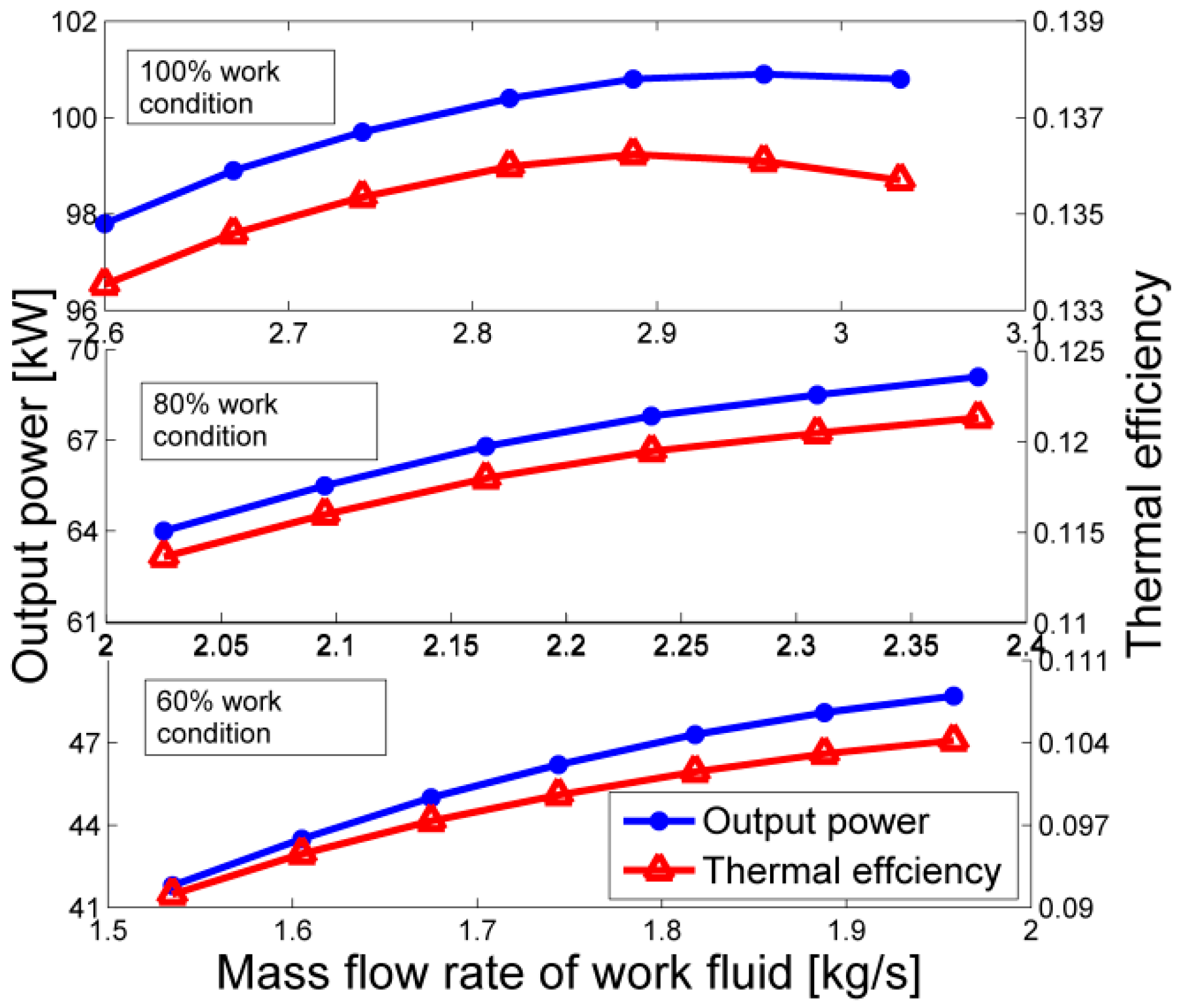
4.1. The Effects of Mass Flow Rate of Hot Water and Working Fluid at Different Working Conditions

Figure 8 and Figure 9 show the effects of working fluid mass flow rate (mf) on degree of superheating, evaporation pressure and isentropic efficiency of the turbine under different working conditions of the gaseous fuel engine. In these figures, including Figure 10, the mass flow rate of hot water remains unchanged. As the working conditions become small, the waste heat amount of exhaust becomes less, so the working fluid mass flow rate must decrease, otherwise the working fluid cannot evaporate totally, which leads to damage to the turbine blades. For every gaseous fuel engine working condition, the max working fluid mass flow rate is the one that makes the degree of superheating become 0 as shown in Figure 8. From Figure 8, it is known that superheat degree decreases with increasing mf, while evaporating pressure rises with it at different working conditions. The turbine is equivalent to a nozzle and when the working fluid mass flow rate increases, more working fluid goes through the turbine, so the pressure before it (evaporating pressure) must get higher.
Figure 10 describes the effects of working fluid mass flow rate on system output power and thermal efficiency. It can be seen from Figure 10 that at 100% working condition the output power and thermal efficiency increase with mf more and more slowly, and finally they show a very small reduction. According to the basic property of ORC [31], the greater the evaporation pressure is, the more output power and thermal efficiency it has. The decreasing degree of superheating has nearly no effect on the thermal efficiency but it leads to a reduction of the output power. The increasing mf and evaporation pressure contribute to the output power, while a decreasing degree of superheating leads to a reduction of the output power. Besides, as is known to all, if the turbine works under part-load conditions, its efficiency will decrease as shown in Figure 9. Therefore, the point where nst is the highest is the design point of the turbine. For these reasons the ORC output power increases and then decreases a little. The thermal efficiency of the ORC increases with evaporation pressure more and more slowly [31], while the turbine isentropic efficiency decreases when mf exceeds the design value, so the thermal efficiency finally also decreases a little. However, under other working conditions of the gaseous fuel engine, because the turbine works under the part-load condition all the time and the increasing mf makes it closer to the design point, the nst rises with increasing mf as shown in Figure 9. Consequently the output power and thermal efficiency also increase with mf all along until mf reaches its maximum value. In a word, Figure 10 indicates that in order to get a large output power and thermal efficiency under different working conditions of gaseous fuel engine, the working fluid mass flow rate should be controlled as large as possible under the condition of no drops at the inlet of the turbine.
Figure 11 shows the effects of hot water mass flow rate on output power and hot water outlet temperature in the exhaust heat exchanger. It can be seen that under different working conditions, the output power almost does not change with the hot water mass flow rate (mw), which means mw cannot improve the system performance. According to the former research [42], the increase of heat source mass flow rate contributes to system output power and thermal efficiency, while a decrease of heat source inlet temperature leads to their reduction. From Figure 11, it is known that the increase of mw brings out the decrease of hot water outlet temperature in exhaust heat exchanger, which is also the heat source inlet temperature of ORC. Therefore, mw almost does not affect system output power and thermal efficiency.
Based on the analysis above, when the working conditions of a gaseous fuel engine change, in order to get a better system performance just the working fluid mass flow rate should be controlled as large as possible with a suitable degree of superheating, leaving alone the hot water mass flow rate. Therefore, a PID controller is used in the ORC system to adjust the working fluid mass flow rate, making the degree of superheating of the working fluid at the end of heating remain constant all the time.

4.2. System Performance with Control

The control result of the degree of superheating of 30 K and working fluid mass flow rate are shown in Figure 12 and Figure 13. In these figures, the working condition of the gaseous fuel engine decrease by 10% every 700 s from 100% to 40%. It can be seen that mf decreases as the working conditions become small and the degree of superheating is positive all along during the dynamic variation process, which ensures the safety of the turbine when the gaseous fuel engine working conditions change. Actually, the degree of superheating can be controlled to be lower. Figure 14 compares the system output power with different controlled degrees of superheating (10 K and 30 K). It can be found that the WHRS with a 10 K degree of superheating always has a greater output power than the system with a 30 K degree of superheating, which proves the conclusion obtained above. With the control of a constant (10K) degree of superheating of the working fluid at the evaporator outlet, the system performance under steady state under seven typical gaseous fuel engine working conditions (100%, 90%, 80, 70%, 60%, 50%, 40%) are shown in Figure 15, Figure 16 and Figure 17.
Figure 15 shows the isentropic efficiency of the turbine (nt), the pump (np) and the thermal efficiency of the ORC (n). It can be found that as the working conditions decease, nt, np and n all become small, especially nt and np which decrease faster and faster. As mentioned above, when the gaseous fuel engine working conditions go down, the exhaust waste heat amount decreases, therefore, the working fluid mass flow rate must be reduced and the reduction of mf leads to the decrease of Pe. The lower Pe the ORC has, the lower thermal efficiency it has. Added to the decrease of isentropic efficiency of pump and turbine, n decreases as the gaseous fuel engine conditions go down. At 100% working condition n is 12.9%, while n becomes 6.5% under 40% working conditions, which means the WHRS performance suffers a great reduction.
Figure 16 and Figure 17 show the improvement of the combined system (ORC WHRS and the gaseous fuel engine). It should be noticed that the improvement of efficiency in Figure 17 excludes the consumed power of the pump and cooling fans. Under 100% working conditions, the ORC has an output power of 100.06 kW. Excluding the consumed power of the cooling fans and pump, the output power of the combined system is 1076.3 kW (the output power of the gaseous fuel engine is 1000 kW) and the thermal efficiency of the combined cycle is 39.4% (the thermal efficiency of the gaseous fuel engine is 36.55%). The output power and thermal efficiency are thus improved by 7.6% and 7.8%, respectively. This is a great advance. However, under 40% working conditions the output power of the combined system is 409.9 kW (the output power of the gaseous fuel engine is 400 kW) and the thermal efficiency of the combined cycle is 28.18% (the thermal efficiency of the gaseous fuel engine is 27.5%). They are improved by 2.5% and 2.47%, respectively. As mentioned above, the WHRS system performance suffers a great reduction under gaseous fuel engine low working conditions, so the improvement of the combined system also decreases. Under 40% working conditions, the increase of output power is just 9.9 kW according to the calculation. If the heat loss of the heat exchanger, and the efficiency of the electric generator connected to the turbine are considered, the increase of output power will be even less. That means the WHRS has nearly no energy-saving effect anymore. Figure 18 indicates that the exhaust temperature at the outlet of hot water heat exchanger decreases as the engine working condition goes down. Therefore, when the system is designed at rated working conditions, the final exhaust temperature should be higher than acid dew point; otherwise the final exhaust temperature may become lower than acid dew point under some part-load working conditions, which can corrode the equipment.

5. Conclusions

In this paper a dynamic model of an ORC-MC system using water as intermediary fluid for exhaust waste heat recovery of a gaseous fuel engine, which has a rated power of 1000 kW, is established. Using this model, the effect of adjustable parameters on the system performance and effective operation strategy under part-load conditions are analyzed. It is found that the intermediary fluid (hot water) mass flow rate nearly has no effect on output power and thermal efficiency of the WHRS, while the mass flow rate of the working fluid has a great effect on them, so when the working conditions of a gaseous fuel engine changes, in order to get a better system performance just the working fluid mass flow rate should be control as large as possible with a suitable degree of superheating, leaving alone the mass flow rate of hot water. Then, the system performance is compared under different controlled degrees of superheating and the results further prove the control direction suggested before. Finally, with the control of a constant degree of superheating (10 K) of the working fluid at the end of the heating process, the system performance at steady state under seven gaseous fuel engine working conditions (100%, 90%, 80%, 70%, 60%, 50%, 40%) are analyzed and the results indicate that the energy-saving effect of WHRS becomes worse and worse as the working conditions decrease. In particular at 40% working conditions the WHRS has nearly no energy-saving effect any more.

Acknowledgments

This work was supported by National Key Technology Support Program of China (No.2015BAG16B00).

Author Contributions

All the authors contributed to the work in this manuscript. Xuan Wang is the main author who established the ORC dynamic model, performed the model validation and control design and wrote the paper. Hua Tian and Gequn Shu provided support and gave useful suggestions during the whole work. All authors revised and approved the manuscript.

Conflicts of Interest

The authors declare no conflict of interest.

Abbreviations

The following abbreviations are used in this manuscript:
TTemperature (K)
ρDensity (kg/m3)
αHeat transfer coefficient (W/m2·K)
CpSpecific heat (J/kg·K)
mMass flow rate (kg/s)
AArea (m2)
tTime (s)
DDiameter (m)
hSpecific enthalpy (J/kg)
ReReynolds number
NuNusselt number
PrPrandtl number
γvoid fraction (m2/s)
SSlip ratio
μDensity ratio
uVelocity (m/s)
LLength (m)
pPressure (Pa)
xVapor quality
ωRevolution speed (rpm)
ηvVolumetric efficiency
VcylCylinder volume (m3)
V ˙ Volume flow rate (m3/s)
CvTurbine coefficient
WWork (W)
ηstIsentropic efficiency of expander
ηspIsentropic efficiency of pump
ηDynamic viscosity (Pa·s) or liquid fraction or efficiency
csIsentropic gas speed(m/s)
lLiquid
gGas or exhaust
eHeat source (hot water)
cCold
fFluid
iInside
oOutside
wWall
inInlet
outOutlet
rWorking fluid
avgAverage
pPump
sIsentropic
tTurbine
caCooling air
ORCOrganic Rankine Cycle
MBMoving Boundary
WHRWaste Heat Recovery
WHRSWaste Heat Recovery System
MCMedium Cycle
ICEInternal Combustion Engine
ODPOzone Depression Potential
GWPGlobal Warming Potential

References

  1. Charles, S. Review of Organic Rankine cycles for internal combustion engine exhaust waste heat recovery. Appl. Therm. Eng. 2013, 51, 711–722. [Google Scholar]
  2. Aghaali, H.; Ångström, H. A review of turbo compounding as a waste heat recovery system for internal combustion engines. Renew. Sustain. Energy Rev. 2015, 49, 819–824. [Google Scholar] [CrossRef]
  3. Wang, T.Y.; Zhang, Y.J.; Peng, Z.J.; Shu, G.Q. A review of researches on thermal exhaust heat recovery with Rankine cycle. Renew. Sustain. Energy Rev. 2011, 15, 2862–2871. [Google Scholar] [CrossRef]
  4. Chammas, R.E.; Clodic, D. Combined cycle for hybrid vehicles. SAE Pap. 2005. [Google Scholar] [CrossRef]
  5. Ringler, J.; Seifert, M.; Guyotot, V.; Hübner, W. Rankine cycle for waste heat recovery of IC engines. SAE Pap. 2009. [Google Scholar] [CrossRef]
  6. Teng, H.; Regner, G.; Cowland, C. Waste heat recovery of heavy-duty diesel engines by Organic Rankine cycle Part I: hybrid energy system of diesel and Rankine engines. SAE Pap. 2007. [Google Scholar] [CrossRef]
  7. Battista, D.D.; Mauriello, M.; Cipollone, R. Waste heat recovery of an ORC-based power unit in a turbocharged diesel engine propelling a light duty vehicle. Appl. Energy 2015, 152, 109–120. [Google Scholar] [CrossRef]
  8. Quoilin, S.; Lemort, V.; Lebrun, J. Experimental study and modeling of an Organic Rankine Cycle using scroll expander. Appl. Energy 2010, 87, 1260–1268. [Google Scholar] [CrossRef]
  9. Yu, G.; Shu, G.; Tian, H.; Wei, H.; Liu, L. Simulation and thermodynamic analysis of a bottoming Organic Rankine Cycle (ORC) of diesel engine (DE). Energy 2013, 51, 281–290. [Google Scholar] [CrossRef]
  10. Manente, G.; Field, R.; DiPippo, R.; Tester, J.W.; Paci, M.; Rossi, N. Hybrid solar geothermal power generation to increase the energy production from a binary geothermal plant. In Proceedings of the ASME 2011 International Mechanical Engineering Congress and Exposition, Denver, CO, USA, 11–17 November 2011.
  11. Jensen, J.M.; Tummescheit, H. Moving boundary models for dynamic simulation of two-phase flows. In Proceedings of the Second International Modelica Conference, Oberpfaffenhofen, Germany, 18–19 March 2002.
  12. Manente, G.; Toffolo, A.; Lazzaretto, A. An Organic Rankine Cycle off-design model for the search of the optimal control strategy. Energy 2013, 58, 97–106. [Google Scholar] [CrossRef]
  13. Yousefzadeh, M.; Uzgoren, E. Mass-conserving dynamic Organic Rankine cycle model to investigate the link between mass distribution and system state. Energy 2015, 93, 1128–1139. [Google Scholar] [CrossRef]
  14. Wei, D.; Lu, X.; Lu, Z.; Gu, J. Dynamic modeling and simulation of an Organic Rankine Cycle (ORC) system for waste heat recovery. Appl. Therm. Eng. 2008, 28, 1216–1224. [Google Scholar] [CrossRef]
  15. Quoilin, S.; Aumann, R.; Grill, A.; Schuster, A.; Lemort, V.; Spliethoff, H. Dynamic modeling and optimal control strategy of waste heat recovery Organic Rankine Cycles. Appl. Energy 2011, 88, 2183–2190. [Google Scholar] [CrossRef]
  16. Mazzi, N.; Rech, S.; Lazzaretto, A. Off-design dynamic model of a real Organic Rankine Cycle system fuelled by exhaust gases from industrial processes. Energy 2015, 90, 537–551. [Google Scholar] [CrossRef]
  17. Rasmussen, B.P.; Shah, R.; Musser, A.B. Control-Oriented Modeling of Transcritical Vapor Compression Systems. Master’s Thesis, University of Illinois Urbana-Champaign, Champaign, IL, USA, 2002. [Google Scholar]
  18. Jensen, J.M. Dynamic Modeling of Thermo-Fluid Systems. Ph.D. Thesis, Technical University of Denmark, Copenhagen, Denmark, 2003. [Google Scholar]
  19. Milián, V.; Navarro-Esbrí, J.; Ginestar, D. Dynamic model of a shell-and-tube condenser. Analysis of the mean void fraction correlation influence on the model performance. Energy 2013, 59, 521–533. [Google Scholar] [CrossRef]
  20. Horst, T.A.; Rottengruber, H.-S.; Seifert, M.; Ringler, J. Dynamic heat exchanger model for performance prediction and control system design of automotive waste heat recovery systems. Appl. Energy 2013, 105, 293–303. [Google Scholar] [CrossRef]
  21. Hou, G.; Sun, R.; Hu, G.; Zhang, J. Supervisory predictive control of evaporator in Organic rankine cycle (ORC) system for waste heat recovery. In Proceedings of the International Conference on Advanced Mechatronic Systems, Zhengzhou, China, 11–13 August 2011.
  22. Zhang, J.; Zhang, W.; Hou, G.; Fang, F. Dynamic modeling and multivariable control of Organic Rankine Cycles in waste heat utilizing processes. Comput. Math. Appl. 2012, 64, 908–921. [Google Scholar] [CrossRef]
  23. Zhang, J.; Zhou, Y.; Gao, S.; Hou, G. Constrained predictive control based on state space model of Organic Rankine Cycle system for waste heat recovery. In Proceedings of the Chinese Control and Decision Conference (CCDC), Taiyuan, China, 23–25 May 2012.
  24. Benato, A.; Kærn, M.R.; Pierobon, L. Analysis of hot spots in boilers of Organic Rankine Cycle units during transient operation. Appl. Energy 2015, 151, 119–131. [Google Scholar] [CrossRef] [Green Version]
  25. Luong, D.; Tsao, T.-C. Linear quadratic integral control of an Organic Rankine Cycle for waste heat recovery in heavy-duty diesel powertrain. In Proceedings of the 2014 American Control Conference (ACC), Portland, OR, USA, 4–6 June 2014.
  26. Gewald, D.; Siokos, K.; Karellas, S. Waste heat recovery from a landfill gas-fired power plant. Renew. Sustain. Energy Rev. 2012, 16, 1779–1789. [Google Scholar] [CrossRef]
  27. Li, X. Research on Design and Performance Optimization of Diesel Engine Waste Heat Recovery Bottoming System and Key Component. Ph.D. Thesis, Tianjin University, Tianjin, China, 2014. [Google Scholar]
  28. Vaja, I. Definition of an Object Oriented Library for the Dynamic Simulation of Advanced Energy Systems: Methodologies, Tools and Application to Combined ICE-ORC Power Plants. Ph.D. Thesis, University of Parma, Parma, Italy, 2009. [Google Scholar]
  29. Sotirios, K.; Andreas, S. Supercritical fluid parameters in Organic Rankine Cycle applications. Int. J. Thermodyn. 2008, 11, 101–108. [Google Scholar]
  30. Schuster, A.; Karellas, S.; Aumann, R. Efficiency optimization potential in supercritical Organic Rankine Cycles. Energy 2010, 35, 1033–1039. [Google Scholar] [CrossRef]
  31. Meinel, D.; Wieland, C.; Spliethof, H. Effect and comparison of different working fluids on a two-stage Organic Rankine Cycle (ORC) concept. Appl. Therm. Eng. 2014, 63, 246–253. [Google Scholar] [CrossRef]
  32. Quoilin, S.; van Den Broek, M.; Declaye, S.; Dewallef, P.; Lemort, V. Techno-economic survey of Organic Rankine Cycle (ORC) systems. Renew. Sustain. Energy Rev. 2013, 22, 168–186. [Google Scholar] [CrossRef]
  33. Xie, H.; Yang, C. Dynamic behavior of Rankine cycle system for waste heat recovery of heavy duty diesel engines under driving cycle. Appl. Energy 2013, 112, 130–141. [Google Scholar] [CrossRef]
  34. Zhang, J.; Zhou, Y.; Wang, R.; Xu, J.; Fang, F. Modeling and constrained multivariable predictive control for ORC (Organic Rankine Cycle) based waste heat energy conversion systems. Energy 2014, 66, 128–138. [Google Scholar] [CrossRef]
  35. Bamgbopa, M.O.; Uzgoren, E. Quasi-dynamic model for an Organic Rankine Cycle. Energy Convers. Manag. 2013, 72, 117–124. [Google Scholar] [CrossRef]
  36. Shiming, Y. Heat Transfer, 4th ed.; Higher Education Press: Beijing, China, 1998; pp. 162–175. (In Chinese) [Google Scholar]
  37. Zivi, S.M. Estimation of steady-state steam void-fraction by means of the principle of minimum entropy production. J. Heat Trans. 1964, 86, 247–252. [Google Scholar] [CrossRef]
  38. Collier, J.G.; Thome, J.R. Convective Boiling and Condensation, 3rd ed.; Clarendon Press: Oxford, UK, 1994. [Google Scholar]
  39. Ahlgren, F.; Mondejar, M.E. Waste heat recovery in a cruise vessel in the Baltic Sea by using an Organic Rankine Cycle: A case study. J. Eng. Gas Turbines Power 2016, 138, 1–15. [Google Scholar]
  40. Peralez, J.; Dufour, P. Towards model-based control of a steam Rankine process for engine waste heat recovery. In Proceedings of the 2011 IEEE Vehicle Power and Propulsion Conference, Seoul, Korea, 9–12 October 2012.
  41. Li, Y.-R.; Wang, J.-N.; Du, M.-T. Influence of coupled pinch point temperature difference and evaporation temperature on performance of organic Ranking cycle. Energy 2012, 42, 503–509. [Google Scholar] [CrossRef]
  42. Shu, G.; Wang, X.; Tian, H. The performance of Rankine Cycle as waste heat recovery system for a natural gas engine at variable working conditions. SAE Pap. 2016. [Google Scholar] [CrossRef]
Figure 1. System diagram of the ORC-MC.
Energies 09 00527 g001
Figure 2. T-S diagram of ORC-MC.
Energies 09 00527 g002
Figure 3. The discretization model of the water heat exchanger.
Energies 09 00527 g003
Figure 4. Notations used in the moving boundary model.
Energies 09 00527 g004
Figure 5. Model validation. (a) The variation of P in Ref. [11]; (b) The variation of P in the paper; (c) The variation of L1 in Ref. [11]; (d) The variation of L1 in the paper.
Energies 09 00527 g005aEnergies 09 00527 g005b
Figure 6. The optimization of work fluid evaporating pressure.
Energies 09 00527 g006
Figure 7. The dynamic variation of evaporation pressure.
Energies 09 00527 g007
Figure 8. The effects of working fluid mass flow rate on evaporation pressure and degree of superheating.
Energies 09 00527 g008
Figure 9. The effects of working fluid mass flow rate on turbine isentropic efficiency.
Energies 09 00527 g009
Figure 10. The effects of working fluid mass flow rate on output power and thermal efficiency of the ORC system.
Energies 09 00527 g010
Figure 11. The effects of hot water mass flow rate on output power and hot water outlet temperature in the exhaust heat exchanger.
Energies 09 00527 g011
Figure 12. Control result of the degree of superheating.
Energies 09 00527 g012
Figure 13. Control result of the working fluid mass fluid rate.
Energies 09 00527 g013
Figure 14. Comparison of the turbine output power with different controlled degrees of superheating (10 K and 30 K).
Energies 09 00527 g014
Figure 15. The isentropic efficiency of the turbine and pump and thermal efficiency of the ORC.
Energies 09 00527 g015
Figure 16. Output power under different working conditions of the gaseous fuel engine.
Energies 09 00527 g016
Figure 17. Thermal efficiency under different working conditions of the gaseous fuel engine.
Energies 09 00527 g017
Figure 18. The exhaust temperature at the outlet of the hot water heat exchanger.
Energies 09 00527 g018
Table 1. Main parameters of the engine.
ParameterUnitValue
Speedr/min600600600600600600600
Working condition load-40%50%60%70%80%90%100%
Effective powerkW4005006007008009001000
Exhaust temperature°C470515525527530532540
Heat consumption rate of gasMJ/kWh13.0911.7611.0810.5910.2010.269.85
Intake air volume flow ratem3/h1774214524652748312035104180
Exhaust volume flow ratem3/h1911231026542959338038004500
Exhaust mass flow ratekg/s0.690.8340.9581.0691.2211.3721.625
Thermal efficiency of engine%27.530.6132.2533.9835.2935.0836.55
Table 2. The design parameters of the ORC-MC WHRS.
Pump and Turbine
ηv = 0.8Vcyl = 2.7313 × 10⁻⁶ m3
Cv = 0.0064ηs = 0.8
ηsp = 0.8
Evaporator and Condenser Parameters
Di = 0.02 mTeout = 373 K
Do = 0.022 mCw = 385 J/kgK
L = 428.79 mρw = 8960 kg/m3
L1 = 117.90 mP = 2000 kPa
L2 = 75.89 mPc = 230 kPa
L3 = 13.01 mdelta Ts = 10 K
Tein = 433 K

