Harnessing the Flexibility of Thermostatic Loads in Microgrids with Solar Power Generation

Abstract

This paper presents a demand response (DR) framework that intertwines thermodynamic building models with a genetic algorithm (GA)-based optimization method. The framework optimizes heating/cooling schedules of end-users inside a business park microgrid with local distributed generation from renewable energy sources (DG-RES) based on two separate objectives: net load minimization and electricity cost minimization. DG-RES is treated as a curtailable resource in anticipation of future scenarios where the infeed of DG-RES to the regional distribution network could be limited. We test the DR framework with a case study of a refrigerated warehouse and an office building located in a business park with local PV generation. Results show the technical potential of the DR framework in harnessing the flexibility of the thermal masses from end-user sites in order to: (1) reduce the energy exchange at the point of connection; (2) reduce the cost of electricity for the microgrid end-users; and (3) increase the local utilization of DG-RES in cases where DG-RES exports to the grid are restricted. The results of this work can aid end-users and distribution network operators to reduce energy costs and energy consumption.

1. Introduction

The stochastic nature of solar and wind energy resources poses several challenges to the large-scale integration of distributed generation from renewable energy sources (DG-RES) into electricity networks, mainly in terms of reliability and economical feasibility [1,2,3]. The flexibility, i.e., the possibility to adapt or shift the electricity generation profile in time, lost on the generation side due to resource variability needs to be compensated by an increased flexibility of the transmission and distribution systems, of the electricity markets and/or of the demand side [4].

The concept of smart grids encompasses different technical solutions that enable flexibility from other sources, such that consumption and/or generation can be shifted with respect to time. This can be achieved through enhanced monitoring and control functionalities, the use of (electrical and/or thermal) buffers and increased consumer participation through demand response (DR) programs [5,6].

DR can be defined as the set of possible actions voluntarily taken by consumers to change their energy usage—either in terms of quantity or timing—in response to an external control signal; e.g., price, resource availability or network security [7,8,9]. Harnessing demand-side flexibility through DR (some examples of which are given in [7,8,10,11,12,13] within the broader concept of demand-side management (DSM)) has become increasingly important within the framework of smart grids. The wide availability and large thermal capacity of thermostatically-controlled loads (e.g., heating, ventilation and air conditioning (HVAC) systems, refrigerators and water heaters) allows for their flexible operation without negatively impacting equipment performance. The aggregation of these types of end-user loads can sum large amounts of energy and have thus become a valuable flexible resource for the implementation of DR programs [14,15,16,17,18,19,20,21,22].

Harnessing the flexibility of end-users is also a more viable solution when compared to other options, such as electrical storage or network reinforcements. The costs of electrical energy storage systems are still prohibitive and, thus, limit their widespread adoption as a source of flexibility. Power system expansions are time consuming and also require significant investments that could be avoided with proper planning and the implementation of DR programs [9].

The benefits of DR are not exclusive to end-users or network operators, nor are their objectives primarily economical.

Table 1. Objectives for deploying demand-side flexibility.

Objective	Stakeholder(s)	References
Improve system balancing	Transmission system operator (TSO)	[9,17,21,23]
Lower fossil fuel-based generation capacity	TSO	[24,25]
Integrate renewable energy sources (RES)	Distribution system operator (DSO)	[26,27]
	Policy makers
	Advocacy groups
Increase system operation efficiency	DSO	[9,16,28,29]
Reduce energy usage and/or costs	Customers (electricity bill and connection capacity)	[19,27]
	DSO (distribution losses)
Reduce CO${}_2$ emissions	Policy makers	[30]
	Advocacy groups

summarizes different objectives for deploying demand-side flexibility found in the literature and the stakeholders involved.

Another concept aimed at meeting emissions reductions, fostering the integration of DG-RES and tackling the hurdles faced by individual end-users is through smart microgrids. Microgrids have historically been proposed as a solution to overcome issues relating to the dispatch, control and interconnection of small generation close to customer loads in islanded situations (e.g., for emergency/backup power) [31]. In recent times, they have been proposed as the building blocks for implementing smart grid functions in the distribution system [5,32,33,34]. Smart microgrids use enhanced communications and controls on top of power system components to enhance traditional functionalities and provide additional services to the grid when operating in grid-parallel mode. These additional services can help reduce the costs of energy supply and open the electricity markets for the participation of individual end-users through aggregation services [31]. They can also improve the overall power system performance, for instance by integrating DG-RES, managing its intermittency at a local level and optimizing the interface with the external grid to flatten out peaks in consumption or control the infeed of renewables. However, DR within the context of smart microgrids is a topic still to be investigated [35].

Moutis et al. propose planned suburban residential areas to be operated as microgrids with DG-RES and electricity storage to support the reliability of the electricity supply [36]. Because the focus of the aforementioned work was on power quality and stability issues, the control of loads, storage and DG-RES were not considered. The authors of [36] nevertheless mention demand-side management as a topic for further research, concluding from their results that, apart from traditional voltage control, demand-side management may also play an important role in the successful, large-scale deployment of smart microgrids.

Efforts to implement DR have been mostly focused on using the flexibility of thermostatic loads of residential customers [9,11,15,18,37,38,39,40,41]. However, the DR potential of this customer segment in demonstration projects has turned out to be lower than expected due to low participation, limited flexibility of resources, large aggregation requirements and prohibitive entrance costs [41,42,43].

The flexibility of end-users in the commercial and industrial (C&I) sector makes an interesting case for the widespread use of DR programs to enable new paradigms for the operation and planning of smart microgrids. This type of end-user has an overall higher consumption footprint (50%–60% of primary energy consumption [44,45]) and a higher peak demand in comparison with residential customers [24,46]. However, the systematic implementation of DR programs for C&I consumers has been limited. This is despite the fact that the C&I sectors were involved in managing power use through contracts with utilities and network operators since the advent of DR and other demand-side management technologies, as discussed in [8,9,37,46]. Some reasons for the limited systematic implementation of DR in the C&I segment are: (1) C&I customers’ individual energy needs and opportunities vary greatly from one another; (2) applications are either restricted in scope or related to ad hoc solutions for a particular industry or location; and (3) there is a lack of consideration and/or documentation of the lessons learned in previous projects [34,46].

An additional limiting factor of the systematic deployment of DR for C&I end-users is that quantifying and unlocking the flexibility of these customers is not always straightforward and requires, in many cases, the support of an extensive data collection framework and a deep understanding of processes inherent to the industry or the specific customer site [46,47,48]. Flexibility can be defined as a function of the available appliances, the nature of the loads and the objectives of flexibility deployment [43]. The problem is that most methods for quantifying flexibility are ex-post and based on the measurement results of very specific projects. Wattjes et al. look at a “quick and dirty” method to quantify flexibility through an ex-ante method by generalizing primary and secondary process loads in C&I premises, but it does not give a very precise indication of the flexibility of each type of load; only whether it could potentially be steered or not [49].

Flexibility can be quantified as a percentage of peak load reduction, but the amount and nature of the peak load needs to be known ex-ante in order to be able to determine what the impact of the flexibility is. This means that there is no input-output relationship given between flexibility and the nature of the loads. Furthermore, knowing the average percentage of flexibility does not guarantee that the flexibility will be available at critical peak moments. How the flexibility is deployed (i.e., what the optimization objectives are) also influences the DR actions that need to be taken.

Existing top-down approaches to quantify flexibility potential for DR, such as those found in [18,29,50,51,52], are very valuable for traditional market players, such as energy suppliers and/or system operators with access to plentiful aggregated historical data, but no way to know what the system characteristics of each individual end-user are. However, one downside of the data-driven approach is that the link between historical and present/future usage could be compromised by a changing system infrastructure and operation, vis-à-vis DG-RES, electric vehicles, storage and other emerging technologies. Such historical data may also not be readily available, including the case of new buildings and business parks. Therefore, we propose a bottom-up, physical modeling approach that is complementary to data-based approaches and that could be useful for new market entities in the power system, such as (microgrid) aggregators, who do not necessarily have access to historical data, but do have access to the technical characteristics of the field devices they control on the supply and demand side.

Bottom-up physical modeling approaches used to determine DR potential from loads’ physical constraints are documented in [53]. The authors of [53] use physical models of household appliances to create aggregate profiles of prototypical residential dwellings, which they use, in conjunction with ambient temperature values, to train piecewise linear regression models to represent DR potential as a function of ambient temperature. Although the DR potential is based on arbitrary testing of different temperature setpoints within a certain comfort range and therefore no optimal temperature settings are achieved, this approach is very useful when dealing with large aggregations (in the order of thousands) of homogeneous buildings, but is not applicable in the business-park microgrid domain due to the heterogeneous nature of the buildings located in these types of areas. Another shortcoming of the DR potential assessment in works such as [53,54] is that, although their modeling approaches are very thorough, their DR quantification methods are based on load response scenarios that are neither dynamic nor optimal.

There are some works in the literature [27,29] that do combine an optimization framework with either a top-down [29] or a bottom-up [27] approach to assess DR potential. However, in order to determine the optimal building load schedule that will yield minimum electricity costs, they require solving two optimization problems ex-ante (energy minimization and energy maximization) to get the maximum and minimum power constraints for the main optimization problem. This approach is useful for small-scale problems with one or few building loads, but does not scale well to the microgrid domain, nor does it consider DG-RES scheduling. Here, we argue for a different methodology that enables us to optimize the load and DG-RES schedules for all customers inside a microgrid simultaneously under a single optimization problem. This is especially important when applied to microgrids with heterogeneous customer types and DG-RES.

In this paper, we propose an automated demand response framework that intertwines the domains of thermal systems and power systems by connecting the thermal dynamics of large buildings to their energy use. We test the proposed DR framework with a case study of a refrigerated warehouse in combination with an office building located in a business park with local PV generation. Our framework iteratively interfaces thermodynamic models of C&I customer premises with an optimization algorithm to show the link between energy flexibility and thermal loads; i.e., how flexibility can be harnessed from customer sites with thermostatic loads and what are the resulting benefit in terms of energy efficiency and cost. The DR framework we propose enables:

• The operation of C&I areas as grid-connected smart microgrids in order to support the local use of DG-RES through flexible demand, optimize multiple building schedules at the same time through a common goal and create benefits for the stakeholders involved.
• The unlocking of the flexibility of thermostatic loads from commercial and industrial (C&I) consumers as the main source for reshaping consumption.

The DR implementation we propose aims to: (1) follow DG-RES production in a grid-connected business park microgrid in order to minimize either energy consumption or cost; and (2) treat DG-RES as a curtailable resource, preparing the ground for situations where the interface between the microgrid and the rest of the distribution grid is constrained.

The main contribution of this paper, thus, is that it combines an optimization-based demand response tool with a bottom-up physical modeling approach to highlight the relationship between flexibility and the nature of the loads independently from historical load data.

The rest of this paper is organized as follows: the motivation for this work and the methodology used are discussed in Section 2. The case study is described in Section 3. Numerical results are given in Section 4 and discussed in Section 5. Finally, conclusions and directions for future work are discussed in Section 6.

2. Methodology

This section first lists the main assumptions and methodology used for (1) the thermodynamic models of C&I buildings and (2) the modeling optimization framework. It also describes the interaction between the two models.

2.1. Assumptions

The scope of the work focuses on quantifying flexible electricity consumption and cost savings related to the heating or cooling processes in C&I end-user sites. For the purposes of this work, we define load flexibility as the ability of loads to be shifted in time by automated DR actions. This means that the loads are neither reparametrized nor curtailed, but rather only hastened or delayed depending on an external control signal. Human interactions with the loads are not considered as part of the flexible load used for our DR program, given that end-user behavior does not account for the main consumption in refrigerated warehouses or other types of industrial loads.

All loads that are not shiftable are considered a part of the buildings’ inflexible baseload, i.e., the processes occurring in the building that are uncontrollable or uninterruptible in nature, and are neglected for the electricity consumption and cost calculations in this study. We assume ventilation gains/losses, as well as internal heat gains from lighting, people and equipment to be constant and, therefore consider the heating or cooling load required to balance out these gains and losses as part of the baseload of our buildings.

We assume that the mechanical heating or cooling system of the buildings has the same principle of operation as a heat pump with a forced air distribution system. We also assume that the forced air distribution system has a constant mass flow rate and is able to maintain a constant air supply temperature.

The heat transfer mechanisms we consider in our building model are conduction and convection. We consider radiative heat transfer as negligible compared to convective heat transfer due to the forced air distribution system of the mechanical heating/cooling system. This is because building materials have generally low emissivity values, and the working temperature differences between the indoor air, the building materials and the ambient are relatively low.

We also assume that all physical and thermal properties of building materials, as well as the indoor and ambient air remain constant, on the grounds that the temperature ranges we are working with are relatively small for any significant change in physical or thermal properties to take place.

The optimization framework aims to optimize the mechanical heating/cooling system schedules of the buildings in the smart microgrid on a day-ahead time horizon and with an hourly resolution. We assume that all end-users in the microgrid (consumers, prosumers and producers alike) are price-takers, meaning that they cannot influence the market electricity prices, and that electricity prices are the same for all consumers. We also assume that for the 24-h time horizon, hourly electricity prices can be perfectly forecasted or are either known via a previous agreement with the customer (i.e., through a contract where pricing schemes are stipulated). We do not consider peak capacity pricing schemes in our work, though they will be included in future work. Lastly, we assume that hourly ambient temperature and DG-RES generation values can be forecasted with a reasonable degree of accuracy.

2.2. Thermodynamic Models

The thermodynamics of C&I customer premises can be described by a first-order dynamic system. Reduced-order building models have been extensively proposed in the literature for satisfying different objectives; e.g., to test the effect of new building components [55], to size building components [56], to optimize building operation schedules and controls [26,27,56,57,58] or forecast the energy performance of buildings [27].

We created a generic, lumped parameter resistance/capacitance (RC) circuit model to achieve a better understanding of how the thermal mass of buildings can unlock demand-side flexibility in terms of available shifting power and duration and possible energy/cost savings. This approach has been previously used in [14,20,55,59], among other works, to capture first-order transients without having to perform a heavily-detailed building simulation that would require an extensive previous knowledge of the buildings and their processes. Another advantage of having a relatively simple building model is that it also facilitates the real-time implementation in control systems, such as the optimization framework we propose in this work.

The energy balance at the building level is given by:

$${\left(m{c}_p\right)}_a\frac{d{T}_{in}\left(t\right)}{dt}={\dot{Q}}_{gains}\left(t\right)-{\dot{Q}}_{losses}\left(t\right)+{\dot{Q}}_{mechanical}\left(t\right)$$

(1)

where $m_a$ is the mass of the indoor air, $c_{p,a}$ is the specific heat capacity of air at 0 °C and the product ${\left(m{c}_p\right)}_a$ is the heat capacity of the indoor air in J/K; $d{T}_i\left(t\right)/dt$ is the rate of change in temperature of the indoor air with respect to time in K/s; and ${\dot{Q}}_{gains}$ are the heat gains, ${\dot{Q}}_{losses}$ the heat losses and ${\dot{Q}}_{mechanical}$ the heat supplied or extracted by the building mechanical heating or cooling system, in watts.

Heat gains and losses are broken down into the following categories [60]:

• internal gains due to, e.g., people, products, lighting and/or equipment present in the building;
• transmission gains or losses through the exterior surfaces of the building, such as the roof, walls, floor and windows; and
• infiltration gains or losses due to mechanical ventilation and unintentional leakage through cracks and seams in the building.

As mentioned in the Assumptions section (Section 2.1), infiltration gains and losses are neglected. Rewriting (1) to expand ${\dot{Q}}_{losses}$ and ${\dot{Q}}_{gains}$, we have:

$$\begin{array}{cc}\hfill {\left(m{c}_p\right)}_a\frac{d{T}_{in}\left(t\right)}{dt}& ={\dot{Q}}_{internal}\left(t\right)+{\dot{Q}}_{transmission}\left(t\right)+{\dot{Q}}_{mechanical}\left(t\right)\hfill \end{array}$$

(2)

The calculation method for each of the terms in (2) will be discussed in the following subsections.

2.2.1. Transmission Gains

Transmission gains through the building envelope are the heat flows between the indoor and ambient environment through each building envelope element n (i.e., the building walls, roof, floor and windows):

$$\begin{array}{c}\hfill {\dot{Q}}_{transmission}=\frac{T_{in}\left(t\right)-T_{amb}\left(t\right)}{R_{env,tot}}\end{array}$$

(3)

where $R_{env,tot}$, given in K/W, is the overall thermal resistance of the building envelope; i.e., the building’s ability to resist heat flows:

$$\begin{array}{c}\hfill R_{env,tot}=\frac{1}{{\sum }_{n=1}^N\frac{1}{R_{conduction,n}+R_{convection,n}}}\end{array}$$

(4)

in which $R_{conduction,n}$ and $R_{convection,n}$ are the total thermal resistances due to each of the heat transfer mechanisms occurring in the building envelope, in K/W.

For each element n of the building envelope:

$$\begin{array}{cc}\hfill R_{conduction,n}& =\frac{L_n}{k_n{A}_n}\hfill \end{array}$$

(5a)

$$\begin{array}{cc}\hfill R_{convection,n}& =\frac{1}{h_{in-env,n}{A}_n}+\frac{1}{h_{env-amb,n}{A}_n}\hfill \end{array}$$

(5b)

where $L_n$ is the material thickness in m, $k_n$ the thermal conductivity coefficient in W/(mK), $A_n$ the heat transfer surface area in m${}^2$ and $h_{in-env,n}$ and $h_{env-amb,n}$ are the convective heat transfer coefficients in W/(m${}^2$K) between the building envelope element and the indoor air or the ambient, respectively. The convective heat transfer coefficient values are experimentally determined and dependent on air velocity, flow regime and surface roughness of the building material. Common values for different types of heat transfer media and surfaces can be found in [60,61].

The time constant of the building envelope is given by ${\tau }_{env}=\left(R_{env,tot}{C}_{env,tot}\right)$, where $C_{env,tot}$ is the overall thermal capacitance of the building; i.e., the building’s capacity to store heat:

$$\begin{array}{c}\hfill C_{env,tot}=\sum _{n=1}^N{m}_n{c}_{p,n}\end{array}$$

(6)

with $m_n$ being the mass of building envelope element n in kilograms and $c_{p,n}$ the specific heat capacity of the material, in J/(kgK).

2.2.2. Internal Gains

As mentioned in the Assumptions section, internal gains from lighting, people and equipment are assumed to be inflexible (i.e., part of the baseload) and are therefore neglected in the building model. Product gains, in the case of the refrigerated warehouse, are not negligible, however, as they account for most of the cooling load of the system and are given by:

$$\begin{array}{c}\hfill {\dot{Q}}_{product}={\left(m{c}_p\right)}_p(T_p\left(t\right)-T_{in}\left(t\right))\end{array}$$

(7)

with $m_p$ and $c_{p,p}$ being the mass in kilograms and specific heat capacity in J/(kgK) of the refrigerated product. Product temperature changes at a rate:

$$\begin{array}{c}\hfill \frac{d{T}_p\left(t\right)}{dt}=\frac{T_{in}\left(t\right)-T_p\left(t\right)}{R_p{C}_p}\end{array}$$

(8)

where $R_p=1/\left(h_{in-p}{A}_p\right)$ is the thermal resistance between the product and the indoor air; $h_{in-p}$ the convective heat transfer coefficient between the product and the indoor air; $A_p$ the surface area of the product exposed to the refrigerated air; and $C_p={\left(m{c}_p\right)}_p$ the thermal capacitance of the product.

Refrigerated warehouses have a lightweight construction with a high insulation value, which means that the thermal mass, i.e., the materials’ inertia against temperature fluctuations, of the building envelope will be low. The bulk of the thermal mass in the refrigerated warehouse is due to the thermal capacitance of the products it stores.

2.2.3. Contribution of the Mechanical Heating/Cooling System

We assume that the mechanical heating or cooling system of the buildings has the same principle of operation as a heat pump with an air distribution system. The heating/cooling capacity of the mechanical system (i.e., the heat supplied or extracted by the building’s mechanical heating or cooling system) is given by:

$${\dot{Q}}_{mechanical}\left(t\right)={\left(\dot{m}{c}_p\right)}_a(T_{supply}-T_{in}\left(t\right))$$

(9)

where ${\dot{m}}_a$ is the mass flow of the conditioned air, $c_{p,a}$ is the specific heat capacity of air and $T_{supply}$ is the temperature of the conditioned air, all of which we assume constant.

The thermodynamic efficiency of the conversion of electrical power into mechanical power by the heat pump’s compressor is given by the coefficient of performance (COP). Also known as the energy efficiency ratio (EER) in cooling applications, the COP is defined, in steady-state operation, as the ratio of heat supplied to or extracted from the building to the electrical power consumed by the heat pump or refrigeration system at a nominal temperature. In reality, the COP, similarly to the heating/cooling capacity of the mechanical system, is dependent on the difference between the the ambient temperature and the conditioned air supply temperature. This means that temperature dynamics are not taken into account with a nominal COP value, and energy performance in practice will be inferior if ambient temperatures deviate too far from the nominal temperature.

While [26,55,58] acknowledge the importance of variable COP, limitations with the black-box simulation software they employed precluded them from modeling a variable COP. We adapted the work of [56,62], where COP for heating and cooling were modeled as a quadratic function for a fixed supply temperature based on regressions from catalog data. In [62], the COP was modeled as a function of the heat source temperature. In [56], the COP was modeled as a function of the ratio between the supply temperature and the temperature difference between supply temperature and heat source. In our work, we approximate the COP as a quadratic function of the conditioned air supply and ambient temperatures, as described in (10):

$$COP(T_{amb}\left(t\right),T_{supply})=b_0+b_1{T}_{amb}\left(t\right)+b_2{T}_{supply}+b_3{T}_{amb}{\left(t\right)}^2+b_4{T}_{supply}^2+b_5{T}_{amb}\left(t\right)T_{supply}$$

(10)

2.2.4. Thermodynamic Model Building Blocks

The building thermodynamics were modeled in MATLAB-Simulink/Simscape by splitting the system into two submodels:

• Building submodel, in which the geometrical characteristics, as well as the physical and thermal properties of the building materials are captured.
• Mechanical heating/cooling system model.

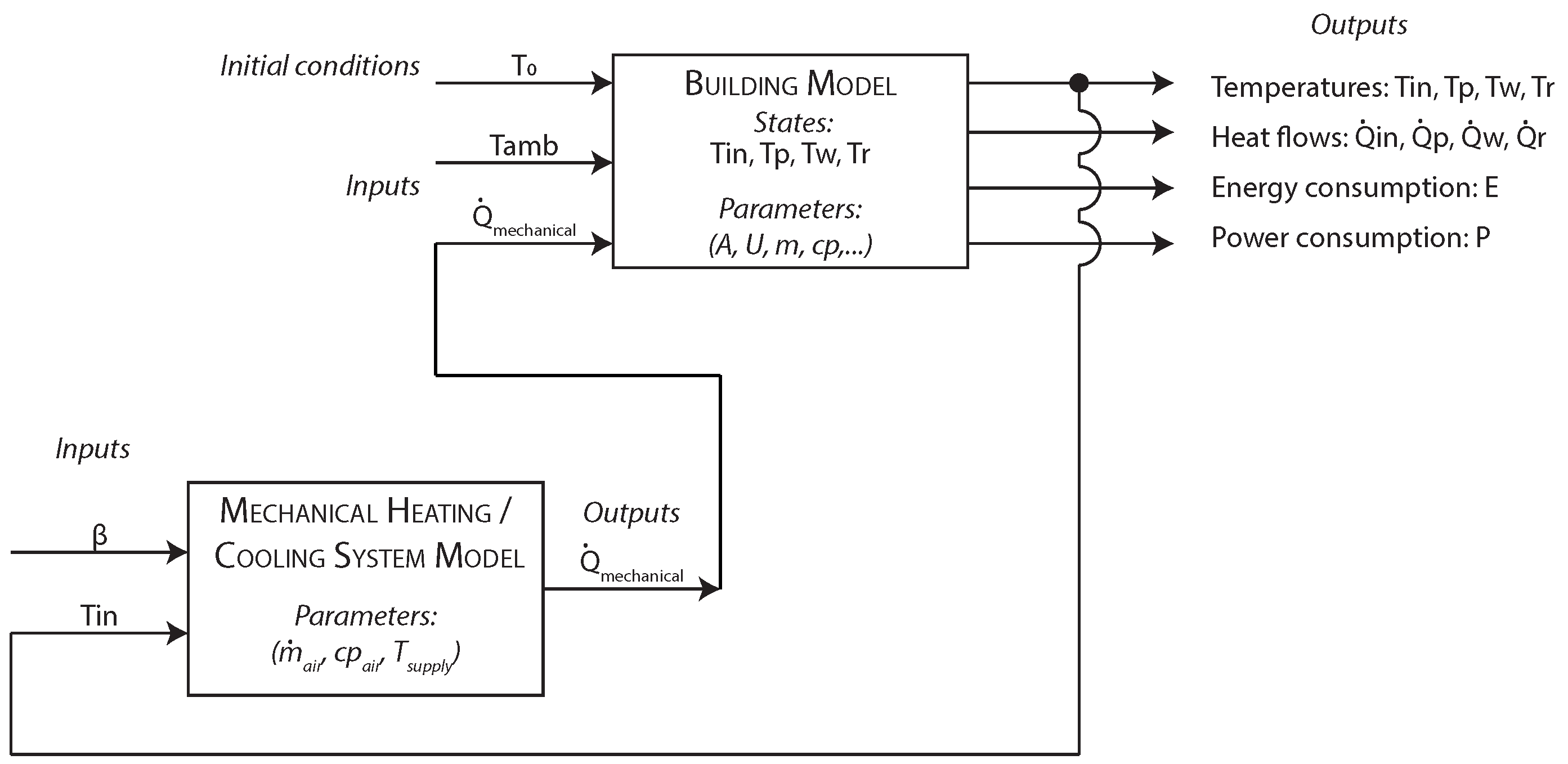
The inputs and outputs of the thermodynamic submodel of a C&I building are shown in Figure 1. The inputs to the mechanical heating/cooling system submodel are functions of time and are:

• an ON/OFF signal to the heating/cooling system, denoted by β in Figure 1; and
• the indoor temperature of the building, denoted by $T_{in}$.

The output of the mechanical heating/cooling system submodel is the heat supplied to or extracted from the building by the heat pump/refrigeration system as a function of time, denoted by ${\dot{Q}}_{mechanical}$ in the diagram.

The inputs to the building submodel are:

• ${\dot{Q}}_{mechanical}$, from the mechanical heating/cooling system submodel; and
• the ambient temperature as a function of time, denoted by $T_{amb}$.

The building submodel’s states are the different temperatures of the building envelope and its contents: temperature of the indoor air, temperature of the products stored (in the case of the refrigerated warehouse) and the temperatures of the different elements of the building envelope. The model also requires some initialization parameters, which include the geometrical and material characteristics of the building and the initial states of the temperatures of the different components.

Apart from the different system temperatures, the outputs of the building submodel are the heat flows in each section of the building envelope and its contents and the power consumption of the building as a function of time, plus the total energy consumption of the building over the designated time horizon.

Section 3 gives the parameters used to populate the model for the case study that we developed.

2.3. Optimization Modeling Framework

This section describes the optimization modeling framework problem formulation. We combine the thermodynamic models of C&I buildings with an optimization modeling framework to show the link between energy flexibility and building temperature settings; i.e., how flexibility can be harnessed from customer sites with thermostatic loads and what the benefits are in terms of energy efficiency and cost.

2.3.1. Problem Formulation

Let us consider that the ON/OFF signal of the mechanical heating or cooling system of end-user i at time t is defined by the binary variable $\beta (i,t)$. Let us also consider that the electricity consumption of the mechanical heating or cooling system of end-user i at time t is given by $E(i,t)$. The net energy imported from the grid of all I end-users connected to the business park microgrid, $E_{net}\left(t\right)$, after the predicted contribution of local DG-RES in the microgrid $E_{RES}\left(t\right)$ at time t is given by:

$$\begin{array}{cc}\hfill E_{net}\left(t\right)& =\sum _{i=1}^I\beta (i,t)E(i,t)-E_{RES}\left(t\right)\hfill \end{array}$$

(11)

The optimization problem is to choose the switching schedules ($\beta (i,t)$) and PV production schedule ($E_{RES}\left(t\right)$) over the whole time horizon, such that either energy consumption (13) or energy cost (14) are minimized; the building temperatures ($T_{in}(i,t)$) will not exceed the critical values determined by the end-users (12b); and local renewable energy exports from the microgrid to the distribution grid are curtailed (12c). The optimization problem is also subject to the physical constraints of local energy generation from renewables in the microgrid (12d). The optimization problem takes on the form:

$$\begin{array}{cc}\hfill {\displaystyle \underset{\beta ,E_{RES}}{min}}& {\displaystyle \mathrm{\Omega }=\mathrm{\Phi }}\hfill \end{array}$$

(12a)

$$\begin{array}{cc}\hfill \mathrm{s}.\mathrm{t}.& T_{min}(i,t)\le T_{in}(i,t)\le T_{max}(i,t)\forall i,t\hfill \end{array}$$

(12b)

$$\begin{array}{c}{E}_{net}\left(t\right)\ge 0\forall t\hfill \end{array}$$

(12c)

$$\begin{array}{cc}& 0\le E_{RES}\left(t\right)\le E_{RES}^{max}\left(t\right)\forall t\hfill \end{array}$$

(12d)

In the energy consumption minimization problem,

$$\mathrm{\Phi }=\sum _{t=1}^T{E}_{net}\left(t\right)$$

(13)

In the energy cost minimization problem:

$$\mathrm{\Phi }=\sum _{t=1}^T\lambda \left(t\right)E_{net}\left(t\right)$$

(14)

with $\lambda \left(t\right)$ being the predicted retail price of electricity at time t.

Constraint (12b) determines the flexibility of the building and enforces the critical temperature ranges for each customer, $T_{min}(i,t)$ and $T_{max}(i,t)$. The values of $T_{in}(i,t)$ are obtained from the thermodynamic building submodels. Constraint (12c) enforces the restriction of local DG-RES exports from the microgrid to the distribution grid. Constraint (12d) enforces the physical upper and lower bounds of local DG-RES production.

The binary variable β makes the problem mixed-integer, which is why we turn to (meta)heuristic methods in general, and genetic algorithms in particular, to solve the optimization problem.

2.3.2. Proposed Genetic Algorithm-Based Control

Although there are many control strategies being developed, there is still room for improvement, and one of the suggestions found in the literature is to use metaheuristic optimization algorithms to improve the performance of DG-RES and DR in microgrids [35]. Genetic algorithms (GA) are an evolutionary optimization approach that iteratively searches for an optimal value of a certain fitness function over randomly-selected points in the definition domain [63]. GA are advantageous to use in nonlinear mixed-integer problems, especially when handling integer variables. Additionally, because they handle multiple search spaces, GAs scale well to higher dimensional problems, especially if the search is parallelized [63].

The GA-based controller we propose is similar to the work of Zong et al. [26], who used this approach for managing the loads of a single refrigerated warehouse to take advantage of local wind production and reduce costs. Said work was done in the context of the Night Wind pilot project [58]. The design variables of our GA-based control strategy are the switching and DG-RES production schedules, and the objective is to minimize electricity costs or energy for the total optimization time horizon and for multiple customer premises in a microgrid. In [26], the objective function is to minimize electricity consumption costs of a single building by using the indoor temperature of the building as the design variable. Our problem formulation introduces local DG-RES as a curtailable resource for instances where exports to the grid are restricted, while in [26], it is assumed that excess DG-RES production can be fed-in back to the distribution grid.

2.4. Interaction between Thermal Models and Optimization Modeling Framework

Conventional mechanical heating/cooling system temperature controls have a fixed set point temperature and fixed temperature trip points. The compressor switches off when the indoor temperature is lower than the difference between the set point and lower trip point (i.e., at $T_{min}$ for cooling applications and $T_{max}$ for heating applications). It switches on when indoor temperature is higher than the difference between the setpoint and the upper trip point (i.e., at $T_{max}$ for cooling applications and $T_{min}$ for heating applications); and takes the state of the previous time step when indoor temperature falls within the deadband.

However, the fixed-setpoint conditions of the temperature control restrict the flexibility of the thermal loads [51]. By contrast, in order to harness and increase the flexibility of the thermal loads at C&I customer premises, we propose coupling the thermal models with the optimization modeling framework to devise an optimal on/off strategy for the heater or chiller to separately achieve the objectives of (1) minimal cost and (2) maximal energy efficiency and discuss the potential benefits of such a strategy. The resulting multidisciplinary DR framework iteratively intertwines the thermodynamic building model with the GA-based optimization. 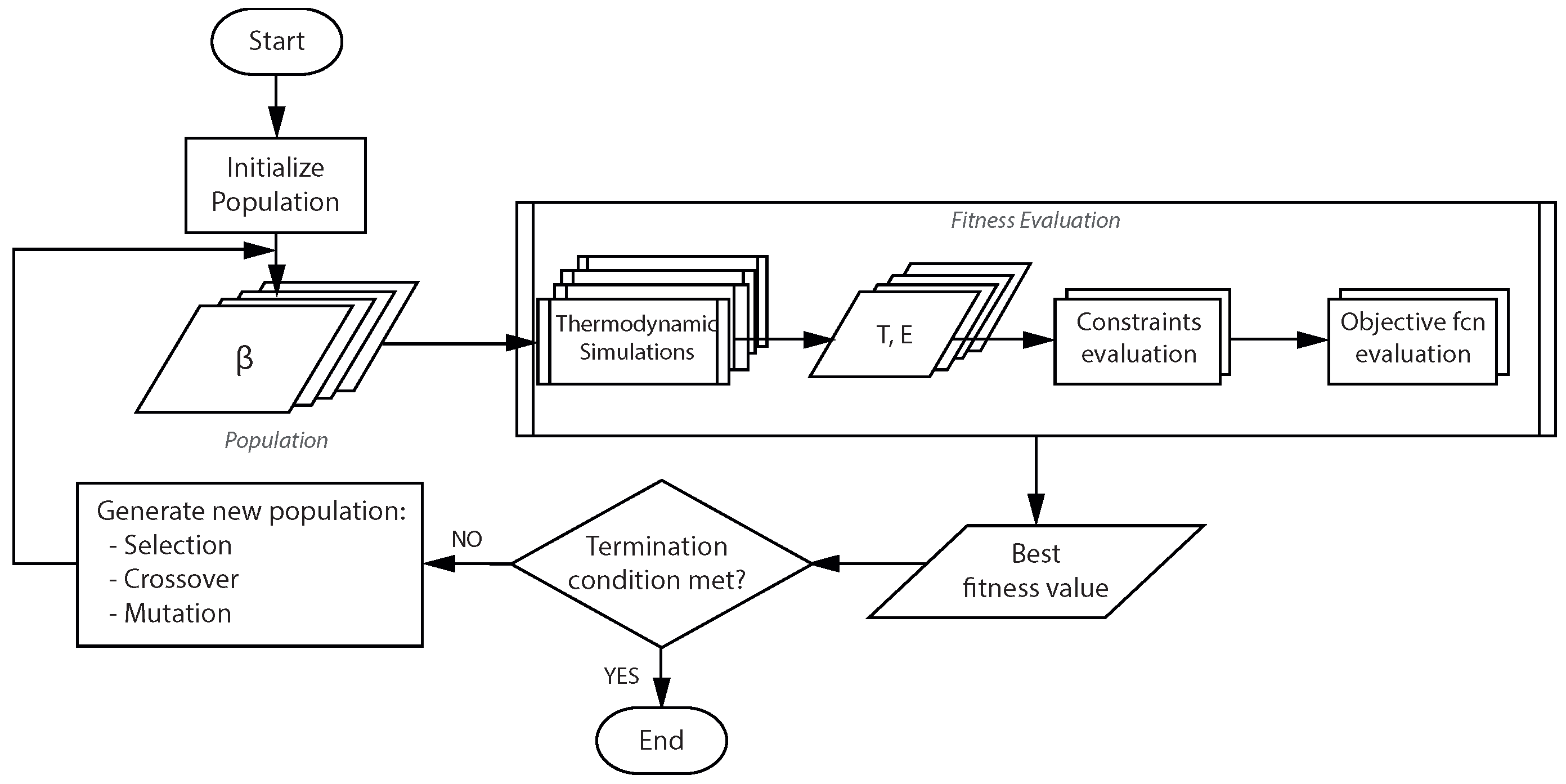Figure 2 visualizes the interactions between the thermal models and the optimization modeling framework.

For every generation in the GA, each individual β in the population of candidate solutions is input into the thermodynamic model to get $T_{in}(i,t)$ and $E(i,t)$. The outputs of the thermodynamic model serve as inputs for the optimization framework, where they are evaluated with respect to the constraints and the objective function. The best individuals of the generation are checked against the termination conditions and used to generate the new population for the next generation if the termination conditions are not met. If the termination conditions are met, the GA ends and returns (1) the optimal β that satisfies the objective function and (2) the objective function value. A block diagram of the GA showing the interaction with the thermal models is shown in Figure 3.

The next section introduces the case study used to test the simulation framework that combines the thermal models with the optimization modeling framework. Numerical results for the case study are given in Section 4 and discussed in depth in Section 5.

3. Case Study

This section describes the case study used to test the interaction of the thermodynamic models with the optimization framework. The case study at hand consists of the business park operated as a grid-parallel microgrid, whose goal is to manage its end-users’ loads and local energy generation in order to (1) minimize end users’ energy costs or (2) maximize local energy consumption from local solar PV generation, per the problem formulation from Section 2.3.1. A refrigerated warehouse and a medium office building are located in the business park.

3.1. Description of Building Characteristics

The office’s building parameters are based on [20,64], though we neglect loads related to user comfort (e.g., moisture control and CO${}_2$ concentration levels) that were considered in [20], on the grounds that we consider them inflexible loads that form part of the building’s baseload.

The refrigerated warehouse is a newly-built, one-story construction, whose building parameters were derived from the reference building stock found in [64]. The design temperature for outdoor conditions of the refrigerating facility are set equal to the 0.4% wet-bulb temperature in the Netherlands: $T_{amb}$ = 20 °C, in accordance with ASHRAEguidelines [60].

The geometrical characteristics, as well as the thermal and physical properties of the materials used to model the refrigerated warehouse and the office building are given in

Table A1. Building parameters.

Parameter	Dimension	Warehouse	Office
Geometric properties
Wall area	m${}^2$	20,840	19,076
Roof area	m${}^2$	32,050	9072
Window area	m${}^2$	0	365
Internal partitions area	m${}^2$	–	11,340
Floor area	m${}^2$	32,050	9072
Floor-to-floor height	m	8.53	10
Gross air volume	m${}^3$	273,387	90,720
Wall thickness	m	0.1066	0.4
Roof thickness	m	0.1286	0.4
Window thickness	m	–	0.1
Internal partitions thickness	m	–	0.0254
Thermal properties
$k_{wall}$	W/(mK)	0.0254	0.038
$k_{roof}$	W/(mK)	0.0254	0.038
$k_{window}$	W/(mK)	–	0.78
$k_{internalpartitions}$	W/(mK)	–	0.16
$c_{p,wall}$	J/(kgK)	701.04	835
$c_{p,roof}$	J/(kgK)	733.34	835
$c_{p,internalpartitions}$	J/(kgK)	–	830
Physical properties
Density, ${\rho }_{wall}$	kg/m${}^3$	146.98	1920
${\rho }_{roof}$	kg/m${}^3$	126.97	32
${\rho }_{window}$	kg/m${}^3$	–	2700

and

Table A2. Convective heat transfer coefficients used for the thermodynamic building models.

Coefficient	Value (W/(m${}^2$K))
Indoor air to wall	24
Indoor air to window	25
Indoor air to roof	12
Wall to ambient	34
Window to ambient	32
Roof to ambient	38
Forced air	2

in Appendix A.

We assume that the refrigerated warehouse serves as a bulk storage cooling facility. By bulk storage facility, it is meant that there is no product in- or out-flow during the 24-h time horizon of the optimization problem. This is a reasonable assumption because the optimization time horizon is less than the storage lifetime of the refrigerated products, which is in the order of weeks or months, depending on the type of product [65]. We assume that the temperature at which the product arrives is equal to the warehouse storage temperature, meaning that the refrigeration system is only used to maintain the product temperature.

Temperature control in both the warehouse and the office occurs with a conventional thermostat. In the business-as-usual scenario, the critical indoor air temperatures of the office building are $T_{min,office}=19$ °C and $T_{max,office}=21$ °C. These limits remain the same for our GA-based controller.

In the business-as-usual scenario, the critical indoor air temperatures of the refrigerated warehouse are $T_{min,warehouse}=1$ °C and $T_{max,warehouse}=3$ °C to keep product temperature stable at around 2 °C. Because the indoor air has less thermal mass than the products stored in the warehouse, indoor air temperatures fluctuate much faster than product temperatures. We propose to use the high thermal mass of the stored products as a source of flexibility.

Industry best practices dictate that product temperature during storage should be kept as stable as possible to avoid the deterioration of product quality and moisture migration of food products [65,66,67], although fluctuations between 1 and 2 °C are permissible [67]. We set the maximum product temperature deviation in the refrigerated warehouse to plus/minus 1 °C with a tolerance of 0.3°, which is well within the 2 °C limit for product quality preservation. Product temperature $T_p$ will be used for the constraints formulation of the optimization problem. This means that $T_p$ will be allowed to oscillate between 1 and 3 ± 0.3 °C in our GA-based controller.

We assume that the products in the warehouse are pelletized and stored in rows of pallets whose surface areas are exposed to forced air cooling. Product directly exposed to the chilled air will be the most sensitive to changes in indoor air temperature. With that in mind, we consider the product temperature to be the temperature at the surface of the pallet and the thermal mass of the product to be the specific heat capacity of the product times the mass of the product on the outer surface of the pallets.

The thermal and physical properties used to model the product inside the refrigerated warehouse are given in

Table 2. Physical and thermal properties of the refrigerated products.

Property	Value
Physical properties
Total volume of product stored, $V_p$	117,560 m${}^3$
Surface area exposed to chilled air, $A_p$	64,077 m${}^2$
Mass of product exposed to chilled air, $m_p$	363,604 kg
Density, ${\rho }_p$	700 kg/m${}^3$
Thermal properties
$k_p$	0.55 W/(mk)
$c_{p,p}$	3851 J/(kgK)

.

3.2. Mechanical Heating and Cooling System Settings

The characteristics of the mechanical cooling and heating systems for the refrigerated warehouse and office building, respectively, are given in

Table 3. Mechanical cooling/heating system characteristics.

Parameter	Unit	Warehouse	Office
Conditioned air mass flow, $\dot{m}$	kg/s	125	0.6
Supply temperature, $T_{supply}$	°C	−5	35

.

Coefficients $b_0$ to $b_5$ used to calculate the COP for the warehouse chiller and office heating system were obtained from catalog values from [68,69], respectively, and are shown in

Table 4. Coefficients for coefficient of performance (COP) calculations.

	COPwarehouse	COPoffice
$b_0$	2.875	3.6853
$b_1$	−0.0425	0.0496
$b_2$	0.14	0
$b_3$	0.000375	−0.0006
$b_4$	0.002775	0
$b_5$	−0.000375	0

.

3.3. Local DG-RES: PV Production

This subsection describes the PV system located on the business park microgrid for use of all end-users of the microgrid. Consider a commercial one kilowatt-peak (kWp), polycrystalline silicone PV module. The theoretical annual yield at standard testing conditions (STC) is 1041.6 kWh/kWp [70]. Using empirical correction factors from [70] to adjust for deviations from STC for conditions in the Netherlands at an optimum orientation angle, we get a yield of 806.3 kWh/kWp. Assuming energy conversion losses of 80% and a module efficiency of 15%, the annual energy yield per square meter of PV panels installed is 98.22 kWh/m${}^2$/year. This means that 8.21 square meters would be required per kWp PV capacity installed.

Assuming there are 1600 square meters available for the installation of PV panels throughout the business park, the total PV capacity installed would be approximately 195 kWp. Solar irradiation values are taken from the Royal Dutch Meteorological Institute (KNMI) archives from a central location in the Netherlands for three representative days in the last 10 years: extreme summer and winter temperatures and a day representing average temperature conditions.

Figure 4 shows the energy production due to PV for the three scenarios of the study. The solid blue line represents the winter PV production profile’ the dashed red line with asterisk markers represents the summer PV production profile’ and the dotted green line with round markers represents the PV production profile for the average temperature scenario. Note that the slight decrease in energy production in the summer PV generation profile that can be observed around noon is most likely due to cloud coverage. The total energy produced over the time horizon for each representative day is tabulated in

Table 5. Maximum PV generation over each representative scenario.

Scenario	$E_{\mathit{RES}}^{\mathit{max}}$ (kWh)
Summer day	1465.3
Winter day	560.53
Average day	874.48

. These values will give the upper bounds for $E_{RES}^{max}$ in the constraint (12 d).

We assume that there is no net-metering scheme nor financial incentive present to feed excess DG-RES production back to the regional distribution grid. For that reason, for the business-as-usual scenario, we curtail excess PV production.

3.4. Electricity Retail Prices

We assume that the microgrid aggregating entity is exposed to dynamic, day-ahead electricity prices and that the end-users connected to the business park microgrid have electricity contracts that follow said prices. Figure 5 plots the hourly electricity prices in €/kWh used for the case study.

3.5. Genetic Algorithm

The design variables of the optimization problem, as mentioned before in Section 2.3.1, are the hourly switching schedules of the mechanical heating or cooling system for all customers, β, and the hourly forecasted DG-RES production schedule, $E_{RES}$. For the 24-hour time horizon of the case study, β has a length of 48 (24 variables per microgrid end-user), and $E_{RES}$ has a length of 24. The resulting phenotype for the GA has 72 elements. Design Variables 1–48 are binary, while Design Variables 49–72 are continuous, whose values are limited by the constraint (12d) in the problem formulation. The fitness function (12a) is subjected to the constraints (12b) and (12c). Additional settings for the GA are as follows: the evolution is limited to 500 generations with a population size of 100 phenotypes; the crossover function rate is set at 0.8. Termination criteria for the GA are a minimum change in the fitness function value of $1\times {10}^{-5}$ and a maximum constraint violation of 0.3.

4. Numerical Results

This section presents the microgrid simulation results for the two optimization objectives formulated in Section 2.3.1—cost minimization and energy minimization—performed in the context of three ambient temperature scenarios for the Netherlands: worst-case summer and winter temperatures and average ambient temperature.

We begin with the business-as-usual (BAU) case, meaning that temperature control is carried out by a conventional thermostat in the buildings and there is no local PV generation, nor any demand-response program in place. We then present the results of the effect of local PV in terms of net cost and energy reduction, but without the effect of DR. Then, we present the effect of DR in our smart microgrid, with regard to the energy consumption and the cost minimization problems solved by our proposed GA-based controller. We compare the optimization results for each temperature scenario (summer, winter, average) to the business-as-usual and PV-with-no-DR scenarios within the framework of the assumptions that we made.

4.1. Business-As-Usual Case

Table 6. Results for the business-as-usual case for three temperature scenarios in the Netherlands.

	Energy (kWh)			€
Scenario	Warehouse	Office	Net load	Total cost
Summer day	3542.7	0.00	3542.7	98.46
Winter day	265.81	1175.1	1440.9	38.79
Average day	1177.6	272.18	1449.78	38.29

shows the results for the BAU case for the business park microgrid, where there is neither local PV generation nor DR.

Table 7. Results for the case illustrating the effect of PV without demand response for three temperature scenarios in the Netherlands.

	Energy (kWh)				€	%
Scenario	Warehouse	Office	PV	Net load	Total cost	Peak reduction	Cost savings
Summer day	3542.7	0.00	976.40	2566.3	68.80	8.77	30.1
Winter day	265.81	1175.1	323.51	1117.4	28.59	0.00	26.3
Average day	1177.6	272.18	341.18	1108.6	28.35	0.82	26.0

shows the effect of having local PV generation in the business park microgrid for each of the three temperature scenarios. From the table, it can be seen that the net load and costs at the point of connection of the microgrid with the regional distribution grid are reduced with respect to the BAU scenario. However, PV by itself does little in general with respect to peak reduction; only in the summer scenario was the peak reduced by approximately eight percent.

4.2. Optimization Framework

This subsection presents the simulation results of the GA-based optimization framework. These results show the effect of DR for both the energy and cost minimization problems on the business park microgrid. Results were obtained by parallelizing the GA computations into eight pools of workers using MATLAB’s Parallel Computing Toolbox. The simulations were carried out using an Intel Core i7-3770 processor running at 3.4 GHz.

It is important to mention that the optimization framework deals with a non-convex combinatorial problem, which means that no global minimum can be guaranteed. We carried out the simulations several times for each scenario and have ported our best results after several iterations of the GA, which means that there could possibly be better solutions for this case than those presented in this work. The outputs of the GA optimization problem are given in

Table 8. GA optimization problem outputs.

Scenario	Objective Function Value	Computing Time (min)	Generations
Energy minimization
Summer day	2139.1	56.1	205
Winter day	723.10	51.1	170
Average day	820.79	64.2	196
Cost minimization
Summer day	54.11	56.3	186
Winter day	18.91	80.0	145
Average day	20.10	66.5	145

.

4.2.1. Energy Minimization

Table 9. Results for the energy minimization problem for three temperature scenarios in the Netherlands.

	Energy (kWh)				(€)	(%)
Scenario	Warehouse	Office	PV	Net load	Total cost	Peak reduction	Cost savings	Energy savings
Summer day	2851.8	86.787	799.44	2139.1	54.13	4.4	21.3	16.7
Winter day	0	1081.6	358.55	723.10	19.58	2.7	31.5	35.3
Average day	1045.4	248.40	473.03	820.79	21.08	0.0	21.3	26.0

tabulates the results of the energy minimization problem. From the table, it can be seen that DR can further improve the energy and cost savings with respect to the scenario with PV, but no DR. The energy minimization problem shifts consumption to the times where PV production is available (see Hours 5–17 in Figure 6), thus reducing the net load seen at the microgrid point of connection with the regional distribution grid and, consequently, the costs.

In the average day scenario, no reductions in peak power were observed. In the summer and winter scenarios, peak reductions of 4.4% and 2.7%, respectively, can be observed.

Figure 6 shows the results for the energy minimization problem in the average temperature scenario. The first subplot shows temperature values for the ambient air (solid yellow line with circle markers), indoor air in the office building and refrigerated warehouse (dashed red line and dotted purple line, respectively), as well as for the products in the refrigerated warehouse (solid blue line). The second subplot shows the optimized switching schedules of the mechanical heating/cooling system of the office (dashed red line) and refrigerated warehouse (solid blue line). Finally, the third subplot shows the energy consumption of the refrigerated warehouse (solid blue line), the office building (dashed red line), the optimized schedule for the PV system (solid yellow line with circle markers), the net energy consumption (dash-dot line with asterisk markers) and the maximum possible PV production over the total time horizon (dotted green line). In the bottom subplot of this figure, it can be seen that consumption has been shifted, inasmuch as possible, to times where PV production is high to keep imports from the electricity distribution grid to a minimum. The flexibility to hasten or delay the load comes from the thermal mass of the buildings.

4.2.2. Cost Minimization

Results for the cost minimization problem for the three temperature scenarios are shown in

Table 10. Results for the cost minimization problem for three temperature scenarios in the Netherlands.

	Energy (kWh)				(€)	(%)
Scenario	Warehouse	Office	PV	Net load	Total cost	Peak reduction	Cost savings	Energy savings
Summer day	2851.8	86.79	800.05	2139.5	54.11	4.4	21.4	16.7
Winter day	0	1111.7	382.32	729.38	18.91	5.2	34.7	34.7
Average day	987.59	230.89	377.47	841.01	20.10	0.0	29.1	24.1

. Figure 7 shows the results of the cost minimization problem for the average temperature scenario, the subplots and legends of which are homologous to those of Figure 6. Table 10 shows the positive effect of DR on energy and cost savings with respect to the scenario with PV, but no DR. Optimization results in terms of cost savings do not differ greatly from the results for the the energy minimization problem, despite the electricity consumption being slightly higher and energy savings being more modest in the cost minimization problem (e.g., consumption increase of 2.4% and savings decrease of 7% in the average temperature scenario). However, the load profile patterns in the cost minimization problem are more spread-out throughout the day to take advantage of both the low prices (see Hours 0–6 in Figure 7) and the availability of PV during the daylight hours (see Hours 5–17 in Figure 7); whereas, in the energy minimization problem, the loads are lumped around the times PV production is high (see Hours 5–17 in Figure 6).

Table 11. PV utilization with and without demand response (DR).

	Local PV Utilization (%)
Case	Summer Day	Winter Day	Average Day	Mean
PV with no DR	67	58	39	54
PV + DR: Energy minimization	55	64	54	61
PV + DR: Cost minimization	55	44	43	47

shows the percentage of local PV utilization under the three temperature scenarios for: the case with PV, but no DR; and the cases with PV and DR. From the table, it can be seen that in the winter and average temperature scenarios, DR can improve the utilization of local PV resources under the energy minimization problem. In the summer scenario, the PV with no DR case has a better local PV utilization ratio than the cases with DR; however, net load and cost are still lower with DR activated. The energy minimization problem has a better local PV utilization ratio because, as mentioned before, the GA optimization harnesses the buildings’ internal thermal masses to shift the loads and cluster them around the times where PV production is occurring, whereas the cost minimization algorithm uses the internal mass of the buildings to spread the loads throughout the day to take advantage of both low electricity prices and PV production times.

Unlike the winter and average temperature scenarios, the PV utilization ratio is the same in the summer scenario for both the energy and cost minimization problems. The similarity of results observed among the summer scenarios can be explained by the fact that there is less load flexibility in the refrigerated warehouse. That is, because the refrigerated warehouse experiences larger heat gains due to the high ambient temperature, the rate of change in product temperature also increases. That means that the chiller has to cycle on and off more frequently to maintain the product temperature stable, leaving less space for the loads to be hastened or delayed.

5. Discussion

This section further discusses the results obtained and their practical implications. The limitations of the work are also discussed in this section.

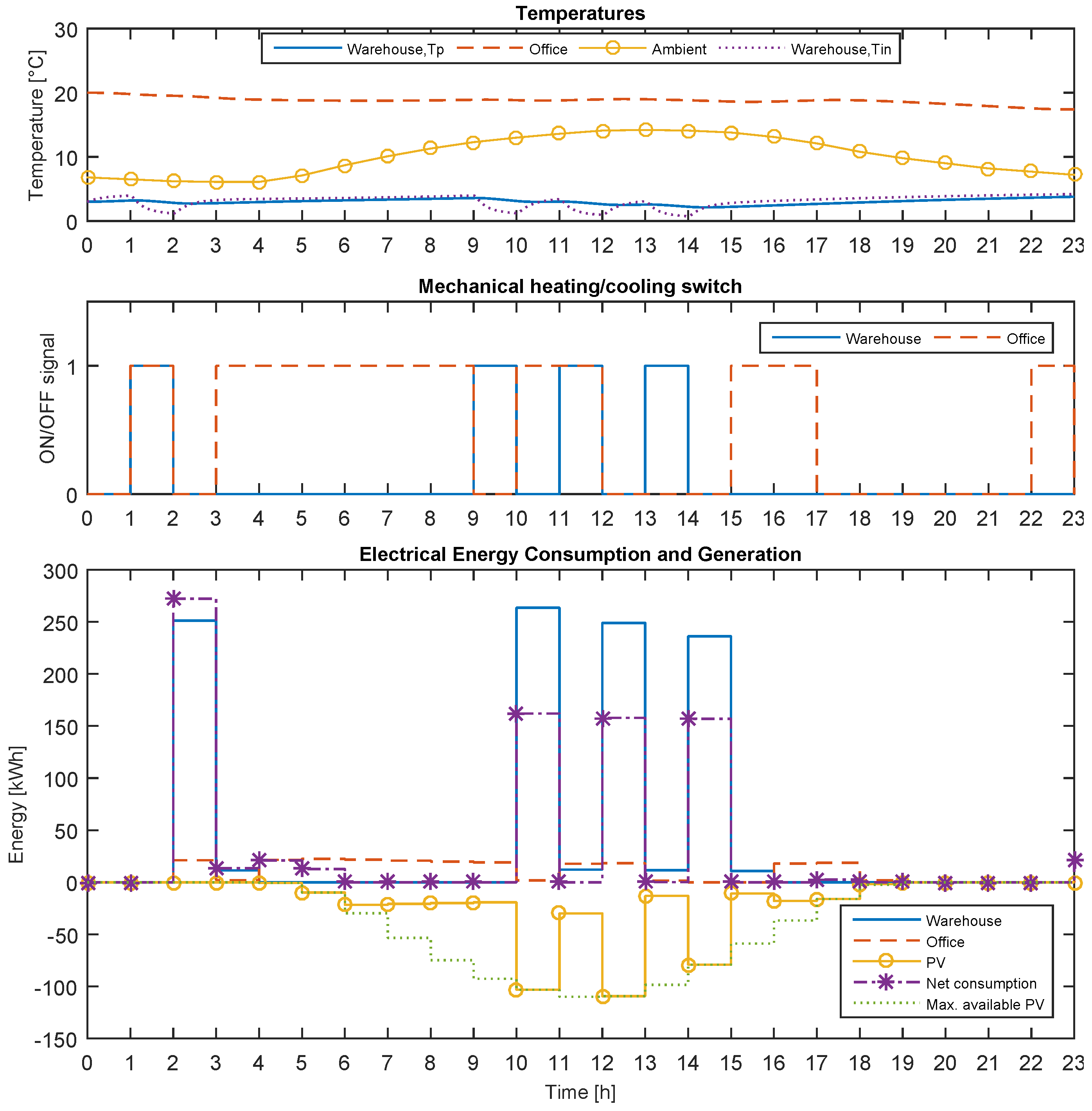
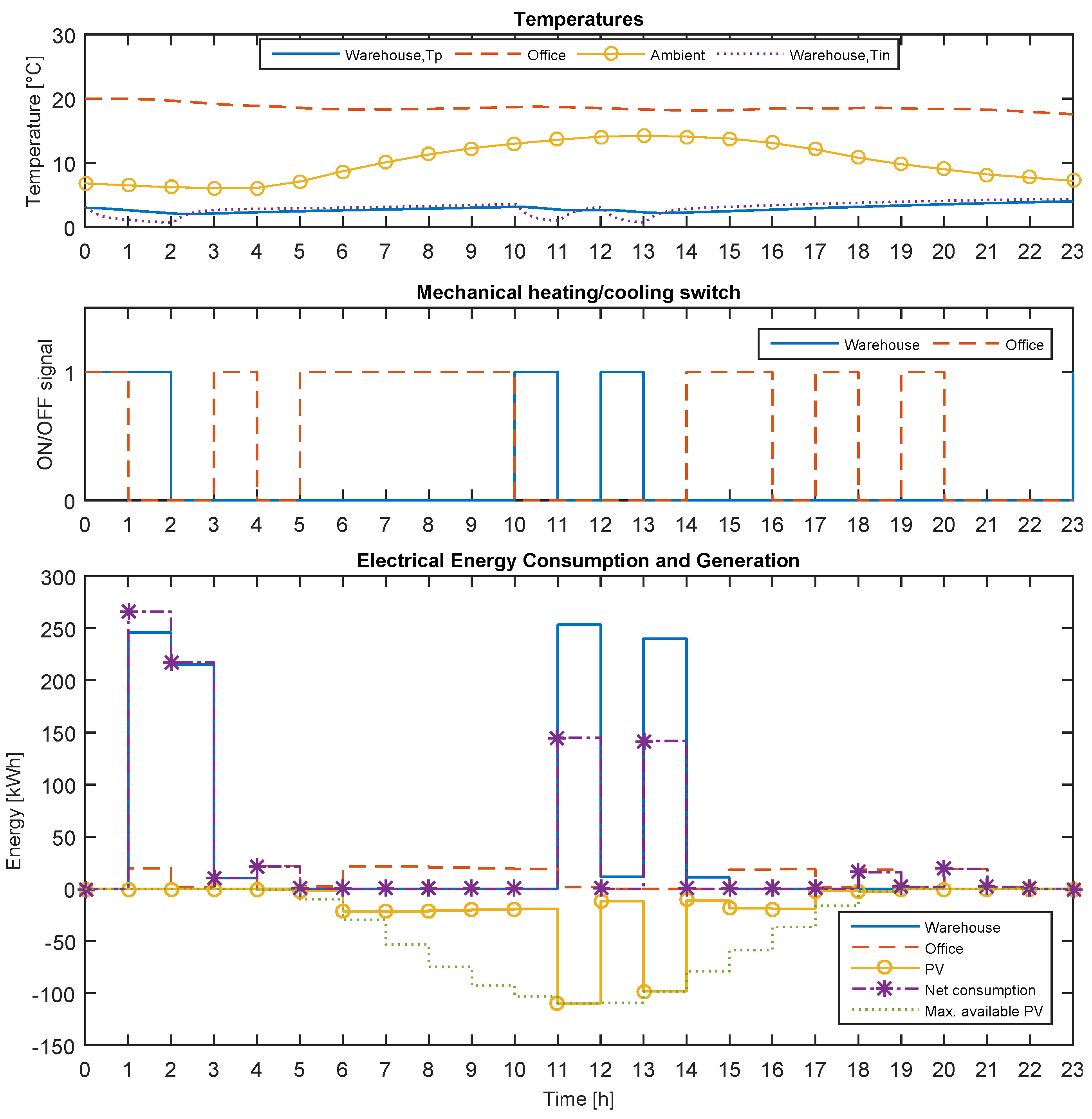
The results obtained show in general terms that DR improves the utilization of local DG-RES by reducing (1) the net apparent load of the microgrid entity at the point of connection with the public electricity grid and (2) the overall cost of energy for the end-users connected to the microgrid. Both DR optimization objectives are an improvement with respect to the BAU scenario and the scenario with PV, but no DR.

Because of the non-convex, combinatorial nature of the optimization problem our DR framework attempts to solve, it is not possible to guarantee that the solution obtained at the end of a given simulation run will be the best one (i.e., a global minimum cannot be guaranteed), but the results presented in this work, based on a number of successive runs from which the best local optimum was selected, show a clear indication of the benefits of this framework.

From the end-users’ perspective, the cost minimization objective for DR is the most desirable, as they pay less for the energy they consume. From the distribution network operator’s perspective, the energy minimization objective for DR in the microgrid is more desirable. In the latter, consumption is shifted to times of high DG-RES production, thereby potentially reducing both peak loads and peak injections.

The ability to curtail DG-RES in our framework only becomes interesting in the event of aging network assets that cannot cope with the large infeed of DG-RES, regulatory frameworks that restrict feed-in due to potential network problems or to avoid negative retail electricity pricing situations. Hence, the applicability of this feature depends on network constraints and also on policy decisions regarding the infeed of DG-RES. Adding network constraints to the model is the first direction that will be explored in our future work.

The results also give insight into the technical potential of using buildings’ internal thermal masses to harness economic benefits for all end-users of the microgrid when using shared resources. Synergies/complementarity between the different loads and DG-RES can be observed from the results, especially for the average (spring/fall scenario). For the summer and winter scenarios, the effect of having diverse users connected to the microgrid is diminished for our particular case study, as almost no energy was being consumed by the refrigerated warehouse in the winter, and the same went for the office building in the summer.

Nevertheless, by pooling shared resources and using DR to reshape the different customer loads to get complementary profiles, we can think of creating local, sustainable ‘energy communities’ in C&I business parks. However, clear contracts or agreements should be put in place on how to distribute these benefits among the end-users, perhaps based on their contribution to reshaping the apparent load profile on the point of connection with the regional electricity grid.

For this framework to be realized in a real-life implementation, an extensive monitoring and control infrastructure needs to be put in place. We also require reliable forecasting methods for DG-RES and temperature, in order to employ the deterministic approach used for the DR framework in this paper. Another precondition required for our model is to have previous knowledge of end-users’ building parameters and characteristics (although not in great detail) to be used as an input for the thermodynamic models. Generic building models can be used to approximate real-life customer sites, but the more information that can be gathered on the building characteristics and processes, the more accurate the simulation results will be.

6. Conclusions

This work presented a multidisciplinary demand response framework that connects the thermal behavior of a building to its energy use by means of a dynamic model and is able to optimize the local energy generation and consumption of all end-users of the microgrid simultaneously. We tested the proposed DR framework with a case study of a refrigerated warehouse and an office building located in a business park with local PV generation in which energy use and electricity costs were optimized in two separate optimization problems.

Results showed the technical potential of DR for C&I customers in terms of: (1) a positive effect of automated solutions for thermostatically-controlled climate; and (2) a positive effect of local use of DG-RES (PV) on the ‘energy community’ as a whole.

Our framework demonstrated that flexibility can be harnessed from customer sites using the buildings’ internal thermal masses in order to: (1) reduce the energy exchange at the point of connection of the microgrid to the regional electricity distribution network; and (2) reduce the cost of electricity for the end-users connected to the microgrid.

The combination of the thermodynamic physical models and the optimization method can be employed as a practical tool in future demonstration projects or commercial endeavors to gain insight on the value of flexibility from C&I loads in concentrated business areas in terms of cost and energy efficiency without the need to resort to expensive field trials. We believe this tool represents a step forward towards the systematic implementation of DR schemes in the C&I domain, especially for end-users clustered as a local energy community that manages their own energy flows.

One possible extension of this work could be not only to set up an interaction framework that defines roles, functionalities and mechanisms within the smart microgrid stakeholders to distribute benefits, but to extend the framework in such a way that it can link and expand the effects of DR in the microgrid to a greater distribution area. Other future directions of the work include: adding network constraints to increase the realism of the model and test its robustness and considering capacity pricing in addition to energy pricing in the cost minimization problem formulation. We also intend to test different mixes of DG-RES (wind and solar) and also consider adding dedicated thermal and/or electrical buffers to test their effect on possible off-grid applications. Adding more types of customers to the microgrid is necessary to test the scalability of our framework. Finally, another possible future direction of the work is addressing the uncertainties inherent in temperature, irradiation and pricing forecasts through a stochastic representation of input data and resulting problem formulation.

References

1. European Commission. Energy 2020: A Strategy for Competitive, Sustainable, and Secure Energy; European Commission: Luxembourg, Luxembourg, 2011. [Google Scholar]
2. European Commission. 2011 Technology Map of the European Strategic Energy Technology Plan; Joint Research Centre-Institute for Energy and Transport: Luxembourg, Luxembourg, 2011. [Google Scholar]
3. Hewicker, C.; Hogan, M.; Mogren, A. Power Perspectives 2030: On the Road to a Decarbonised Power Sector; European Climate Foundation: Den Haag, The Netherlands, 2012. [Google Scholar]
4. Mansoor, A.; Gellings, C.; Schoff, R. Power System Flexibility. Smart Grid 2013. [Google Scholar]
5. European Commission. EUR 22040—European Technology Platform SmartGrids; Office for Official Publications of the European Communities: Luxembourg, Luxembourg, 2006; pp. 1–44. [Google Scholar]
6. EU Commission Task Force for Smart Grids. Expert Group 1: Functionalities of Smart Grids and Smart Meters; European Commission: Brussels, Belgium, 2010. [Google Scholar]
7. IndEco Strategic Consulting. Demand Side Management and Demand Response in Municipalities; IndEco Strategic Consulting: Toronto, ON, Canada, 2004. [Google Scholar]
8. Lampropoulos, I.; Kling, W.L.; Ribeiro, P.F.; van den Berg, J. History of demand side management and classification of demand response control schemes. In Proceedings of the 2013 IEEE Power & Energy Society General Meeting, Vancouver, BC, Canada, 21–25 July 2013; pp. 1–5.
9. Siano, P. Demand response and smart grids—A survey. Renew. Sustain. Energy Rev. 2014, 30, 461–478. [Google Scholar] [CrossRef]
10. Palensky, P.; Dietrich, D. Demand Side Management: Demand Response, Intelligent Energy Systems, and Smart Loads. IEEE Trans. Ind. Inf. 2011, 7, 381–388. [Google Scholar] [CrossRef]
11. Soares, A.; Gomes, A.; Antunes, C.H. Domestic load characterization for demand-responsive energy management systems. In Proceedings of the IEEE International Symposium Sustainable System Technology, Boston, MA, USA, 16–18 May 2012.
12. ENA Electricity Demand Side Response Shared Service Group. Demand Side Response Shared Services Framework; Energy Networks Association: London, UK, 2014. [Google Scholar]
13. Shen, J.; Jiang, C.; Li, B. Controllable Load Management Approaches in Smart Grids. Energies 2015, 8, 1187–11202. [Google Scholar] [CrossRef]
14. Kalsi, K.; Chassin, F.; Chassin, D. Aggregated modeling of thermostatic loads in demand response: A systems and control perspective. In Proceedings of the 2011 50th IEEE Conference Decision Control European Control Conference (CDC-ECC), Orlando, FL, USA, 12–15 December 2011; pp. 15–20.
15. Baghina, N.; Lampropoulos, I.; Asare-Bediako, B.; Kling, W.L.; Ribeiro, P.F. Predictive control of a domestic freezer for real-time demand response applications. In Proceedings of the 2012 3rd IEEE PES Innovative Smart Grid Technologies Europe, ISGT Europe, Berlin, Germany, 14–17 October 2012; pp. 1–8.
16. Klaassen, E.; Zhang, Y.; Lampropoulos, I.; Slootweg, H. Demand side management of electric boilers. In Proceedings of the 2012 3rd IEEE PES Innovative Smart Grid Technologies Europe, ISGT Europe, Berlin, Germany, 14–17 October 2012; pp. 1–6.
17. Vrettos, E.; Koch, S.; Andersson, G. Load frequency control by aggregations of thermally stratified electric water heaters. In Proceedings of the 2012 3rd IEEE PES Innovative Smart Grid Technologies Europe, ISGT Europe, Berlin, Germany, 14–17 October 2012; pp. 1–8.
18. Kara, E.; Tabone, M.D.; MacDonald, J.; Callaway, D.S.; Kiliccote, S. Quantifying Flexibility of Residential Thermostatically Controlled Loads for Demand Response: A Data-driven Approach. In Proceedings of the 1st ACM Conference on Embedded Systems for Energy-Efficient Buildings, Memphis, TN, USA, 5–6 November 2014.
19. Yoon, J.H.; Baldick, R.; Novoselac, A. Dynamic Demand Response Controller Based on Real-Time Retail Price for Residential Buildings. IEEE Trans. Smart Grid 2014, 5, 121–129. [Google Scholar] [CrossRef]
20. Hurtado, L.; Mocanu, E.; Nguyen, P.; Kling, W. Comfort-constrained demand flexibility management for building aggregations using a decentralized approach. In Proceedings of the SmartGreens 2015—4th International Conference Smart Cities Green ICT System, Lisbon, Portugal, 20–22 May 2015; pp. 157–166.
21. Tindemans, S.H.; Trovato, V.; Strbac, G. Decentralized Control of Thermostatic Loads for Flexible Demand Response. IEEE Trans. Control Syst. Technol. 2015, 23, 1685–1700. [Google Scholar] [CrossRef]
22. Gelažanskas, L.; Gamage, K.A.A. Distributed Energy Storage Using Residential Hot Water Heaters. Energies 2016, 9, 127. [Google Scholar] [CrossRef] [Green Version]
23. Paulus, M.; Borggrefe, F. The potential of demand-side management in energy-intensive industries for electricity markets in Germany. Appl. Energy 2011, 88, 432–441. [Google Scholar] [CrossRef]
24. Grünewald, P.; Torriti, J. Demand response from the non-domestic sector: Early UK experiences and future opportunities. Energy Policy 2013, 61, 423–429. [Google Scholar] [CrossRef]
25. Atia, R.; Yamada, N. Distributed Renewable Generation and Storage System Sizing Based on Smart Dispatch of Microgrids. Energies 2016, 9, 176. [Google Scholar] [CrossRef]
26. Zong, Y.; Cronin, T.; Gehrke, O.; Bindner, H.; Hansen, J.C.; Latour, M.I.; Arcauz, O.U. Application genetic algorithms for load management in refrigerated warehouses with wind power penetration. In Proceedings of the 2009 IEEE PowerTech, Bucharest, Romania, 28 June–2 July 2009; pp. 1–6.
27. De Coninck, R.; Helsen, L. Bottom-up quantification of the flexibility potential of buildings. In Proceedings of the BS2013 13th Conference International Building Performance Simulation Association, Chambéry, France, 25–28 August 2013; pp. 3250–3257.
28. Veldman, E. Power play: Impacts of flexibility in future residential electricity demand on distribution network utilisation. Ph.D Thesis, Eindhoven University of Technology, Eindhoven, The Netherlands, 2013. [Google Scholar]
29. Oldewurtel, F.; Sturzenegger, D.; Andersson, G.; Morari, M.; Smith, R.S. Towards a standardized building assessment for demand response. In Proceedings of the 2013 IEEE 52nd Annual Conference Decision Control (CDC), Florence, Italy, 10–13 December 2013; pp. 7083–7088.
30. Horn, K.E.V.; Apostolopoulou, D. Assessing Demand Response Resource locational impacts on system-wide carbon emissions reductions. In Proceedings of the North American Power Symposium (NAPS), Champaign, IL, USA, 9–11 September 2012; pp. 1–6.
31. Morales González, R.; Wattjes, F.; Gibescu, M.; Vermeiden, W.; Slootweg, J.; Kling, W. Applied Internet of Things Architecture to Unlock the Value of Smart Microgrids. IEEE Internet Things J. 2016, in press. [Google Scholar]
32. Lasseter, B. Microgrids [distributed power generation]. In Proceedings of the IEEE Power Engineering Society Winter Meeting 2001, Columbus, OH, USA, 28 January–1 February 2001; Volume 1, pp. 146–149.
33. Lasseter, R.H. Smart Distribution: Coupled Microgrids. Proc. IEEE 2011, 99, 1074–1082. [Google Scholar] [CrossRef]
34. Ton, D.; Smith, M. The U.S. Department of Energy’s Microgrid Initiative. Electr. J. 2012, 25, 84–94. [Google Scholar] [CrossRef]
35. A. Rahman, H.; Majid, M.S.; Rezaee Jordehi, A.; Chin Kim, G.; Hassan, M.Y.; O. Fadhl, S. Operation and control strategies of integrated distributed energy resources: A review. Renew. Sustain. Energy Rev. 2015, 51, 1412–1420. [Google Scholar] [CrossRef]
36. Moutis, P.; Skarvelis-Kazakos, S.; Brucoli, M.; Hung, J.; Wu, S.W. Planned communities as microgrid applications. In Proceedings of the 2014 IEEE PES Innovative Smart Grid Technology Conference Europe (ISGT-Europe), Istanbul, Turkey, 12–15 October 2014; pp. 1–7.
37. Torriti, J.; Hassan, M.G.; Leach, M. Demand response experience in Europe: Policies, programmes and implementation. Energy 2010, 35, 1575–1583. [Google Scholar] [CrossRef]
38. Lampropoulos, I.; Băghina, N.; Kling, W.L.; Ribeiro, P.F. A predictive control scheme for real-time demand response applications. IEEE Trans. Smart Grid 2013, 4, 2049–2060. [Google Scholar] [CrossRef]
39. Liu, W.; Wu, Q.; Wen, F.; Ostergaard, J. Day-Ahead Congestion Management in Distribution Systems Through Household Demand Response and Distribution Congestion Prices. IEEE Trans. Smart Grid 2014, 5, 2739–2747. [Google Scholar] [CrossRef] [Green Version]
40. D’hulst, R.; Labeeuw, W.; Beusen, B.; Claessens, S.; Deconinck, G.; Vanthournout, K. Demand response flexibility and flexibility potential of residential smart appliances: Experiences from large pilot test in Belgium. Appl. Energy 2015, 155, 79–90. [Google Scholar] [CrossRef]
41. Labeeuw, W.; Stragier, J.; Deconinck, G. Potential of Active Demand Reduction With Residential Wet Appliances: A Case Study for Belgium. IEEE Trans. Smart Grid 2015, 6, 315–323. [Google Scholar] [CrossRef]
42. He, X.; Keyaerts, N.; Azevedo, I.; Meeus, L.; Hancher, L.; Glachant, J.M. How to engage consumers in demand response: A contract perspective. Util. Policy 2013, 27, 108–122. [Google Scholar] [CrossRef] [Green Version]
43. Klaassen, E.; Frunt, J.; Slootweg, J. Method for Evaluating Smart Grid Concepts and Pilots. In Proceedings of the IEEE Young Research Symposium 2014 (YRS 2014), Ghent, Belgium, 24–25 April 2014; pp. 1–6.
44. U.S. Department of Energy. NewsRoom Features—August 2009 Energy Efficiencies in Buildings to Improve Under NETL-Directed ARRA Funding, 2009. Available online: http://www.netl.doe.gov/newsroom/features/08-2009.html (accessed on 10 October 2013).
45. European Energy Agency. Final Energy Consumption by Sector and Fuel (CSI 027/ENER 016), 2015. Available online: http://www.eea.europa.eu/data-and-maps/indicators/final-energy-consumption-by-sector-8/assessment-2 (accessed on 4 March 2015).
46. Samad, T.; Kiliccote, S. Smart grid technologies and applications for the industrial sector. Comput. Chem. Eng. 2012, 47, 76–84. [Google Scholar] [CrossRef]
47. Encinas, N.; Alfonso, D.; Alvarez, C.; Pérez-Navarro, A. Energy market segmentation for distributed energy resources implementation purposes. Gener. Transm. Distrib. IET 2007, 1, 324–330. [Google Scholar] [CrossRef]
48. Álvarez Bel, C.; Ortega, M.A.; Escrivá, G.E.; Gabaldón Marín, A. Technical and economical tools to assess customer demand response in the commercial sector. Energy Convers. Manag. 2009, 50, 2605–2612. [Google Scholar]
49. Wattjes, F.D.; Janssen, S.L.L.; Slootweg, J.G. Framework for estimating flexibility of commercial and industrial customers in Smart Grids. In Proceedings of the 2013 4th IEEE/PES Innovative Smart Grid Technology Europe ISGT Europe, Copenhagen, Denmark, 6–9 October 2013; pp. 1–5.
50. Pielow, A.; Sioshansi, R.; Roberts, M.C. Modeling short-run electricity demand with long-term growth rates and consumer price elasticity in commercial and industrial sectors. Energy 2012, 46, 533–540. [Google Scholar] [CrossRef]
51. Zavala, V.M. Real-time optimization strategies for building systems. Ind. Eng. Chem. Res. 2013, 52, 3137–3150. [Google Scholar] [CrossRef]
52. Albert, A.; Rajagopal, R. Finding the right consumers for thermal demand-response: An experimental evaluation. IEEE Trans. Smart Grid 2016, 99. [Google Scholar] [CrossRef]
53. Yin, R.; Kara, E.C.; Li, Y.; DeForest, N.; Wang, K.; Yong, T.; Stadler, M. Quantifying flexibility of commercial and residential loads for demand response using setpoint changes. Appl. Energy 2016, 177, 149–164. [Google Scholar] [CrossRef]
54. Ghatikar, G.; Mashayekh, S.; Stadler, M.; Yin, R.; Liu, Z. Distributed energy systems integration and demand optimization for autonomous operations and electric grid transactions. Appl. Energy 2016, 167, 432–448. [Google Scholar] [CrossRef]
55. Wilson, M.B.; Luck, R.; Mago, P.J. A First-Order Study of Reduced Energy Consumption via Increased Thermal Capacitance with Thermal Storage Management in a Micro-Building. Energies 2015, 8, 12266–12282. [Google Scholar] [CrossRef]
56. Li, S.; Zhang, W.; Lian, J.; Kalsi, K. On Market-Based Coordination of Thermostatically Controlled Loads With User Preference. In Proceedings of the 53rd IEEE Conference on Decision Control, Los Angeles, CA, USA; 2014; pp. 2474–2480. [Google Scholar]
57. Treado, S.; Chen, Y. Saving Building Energy through Advanced Control Strategies. Energies 2013, 6, 4769. [Google Scholar] [CrossRef]
58. Cronin, T.; Bindner, H.; Zong, Y. Night Wind—Deliverable D.3.2: Main Simulation Report; Risø National Laboratory for Sustainable Energy: Roskilde, Denmark, 2008. [Google Scholar]
59. Zaparoli, E.L.; de Lemos, M. Simulation of Transient Response of Domestic Refrigeration Systems. In International Refrigeration and Air Conditioning; Purdue University: West Lafayette, IN, USA, 1996; pp. 495–500. [Google Scholar]
60. American Society of Heating, Refrigerating, and Air-Conditioning Engineers (ASHRAE). 2009 ASHRAE Handbook—Fundamentals (SI units); ASHRAE: Atlanta, GA, USA, 2009. [Google Scholar]
61. American Society of Heating, Refrigerating, and Air-Conditioning Engineers (ASHRAE). 2006 ASHRAE Handbook: Refrigeration; ASHRAE: Atlanta, GA, USA, 2006. [Google Scholar]
62. Nam, Y.; Ooka, R.; Hwang, S. Development of a numerical model to predict heat exchange rates for a ground-source heat pump system. Energy Build. 2008, 40, 2133–2140. [Google Scholar] [CrossRef]
63. Rojas, R. Neural Networks; Springer-Verlag: Berlin, Germany, 1996. [Google Scholar]
64. U.S. Department of Energy. Reference Buildings by Building Type: Warehouse; U.S. Department of Energy: Washington, DC, USA, 2010.
65. Food and Beverage Stability and Shelf Life; Kilcast, D.; Subramaniam, P. (Eds.) Woodhead: Cambridge, MA, USA, 2011.
66. Çengel, Y.A. Refrigeration and freezing of foods. In Heat and Mass Transfer: A Practical Approach, 3rd ed.; McGraw-Hill: New York, NY, USA, 2007; Chapter 17. [Google Scholar]
67. Dermesonlouoglou, E.; Giannou, V.; Tzia, C. Chilling. In Handbook of Food Processing: Food Preservation; CRC Press: Boca Raton, FL, USA, 2016; Chapter 6; pp. 223–258. [Google Scholar]
68. Stoeckle, R. Refrigerated Warehouse Operation Under Real Time Pricing. Master’s Thesis, University of Wisconsin-Madison, Madison, WI, USA, 2000. [Google Scholar]
69. 10kw EVI Air Source Heat Pumps. Available online: http://air-sourceheatpump.com/products-2/evi-cold-climate-heat-pump/10kw-evi-air-source-heat-pumps/ (accessed on 29 February 2016).
70. Deutsche Gesellschaft für Sonnenenergie. Planning and Installing Photovoltaic Systems : A Guide for Installers, Architects, and Engineers, 2nd ed.; Earthscan: Sterling, VA, USA, 2008; pp. 1–384. [Google Scholar]
Figure 1. Inputs and outputs of the physical model.
Energies 09 00547 g001
Figure 2. Smart microgrid simulation framework: interactions between the physical model and the optimization framework.
Energies 09 00547 g002
Figure 3. Flowchart of the genetic algorithm-based controller.
Energies 09 00547 g003
Figure 4. Solar PV generation for three representative days in the Netherlands.
Energies 09 00547 g004
Figure 5. Dynamic electricity pricing scheme for the end-users of the business park microgrid.
Energies 09 00547 g005
Figure 6. Energy minimization results for the average temperature scenario.
Energies 09 00547 g006
Figure 7. Cost minimization results for the average temperature scenario.
Energies 09 00547 g007