
Electromagnetohydrodynamic Effects on Steam Bubble Formation in Vertical Heated Upward Flow

 and
and 
Abstract
:
1. Introduction
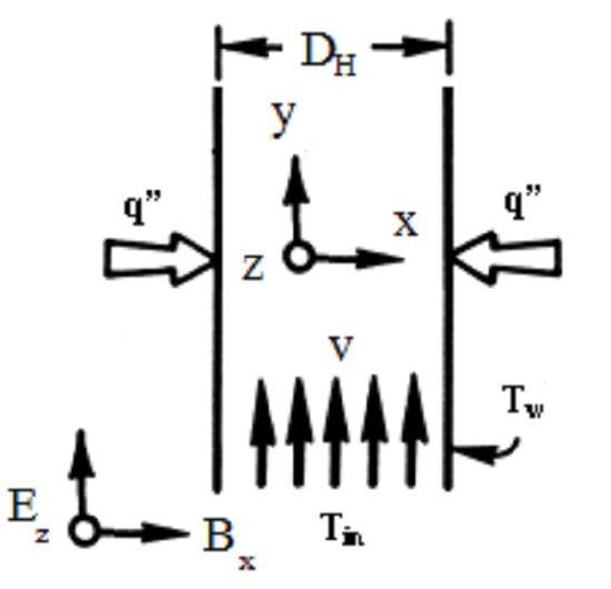
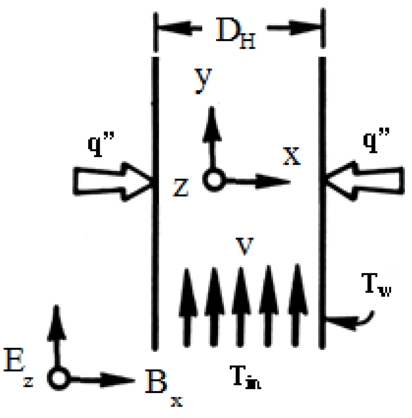
2. Problem Definition
3. Mathematical Model
3.1. Conservation of Mass: Continuity Equation
3.2. Conservation of Momentum
- The Reynolds stresses, viscous stresses and co-variance terms are neglected.
- The surface tension forces are negligible. Therefore, the same pressure for both of the phases and interfacial are assumed.
- The interfacial momentum storage is neglected.
- The interface force terms consist of both pressure and viscous stresses.
- The constant area is assumed.
- The virtual mass formulation is used (for the more stability in the numerical solution, the continuity equation at each phase is multiplied by a percentage of the corresponding phase velocity, and the consequential equation is subtracted from the related momentum equation).
3.3. Conservation of Energy
4. Numerical Procedure
5. Results and Discussion
6. Conclusions
- To get a correct understanding of the mechanism of heat transfer enhancement in the present investigation, the system was studied in a steady state condition.
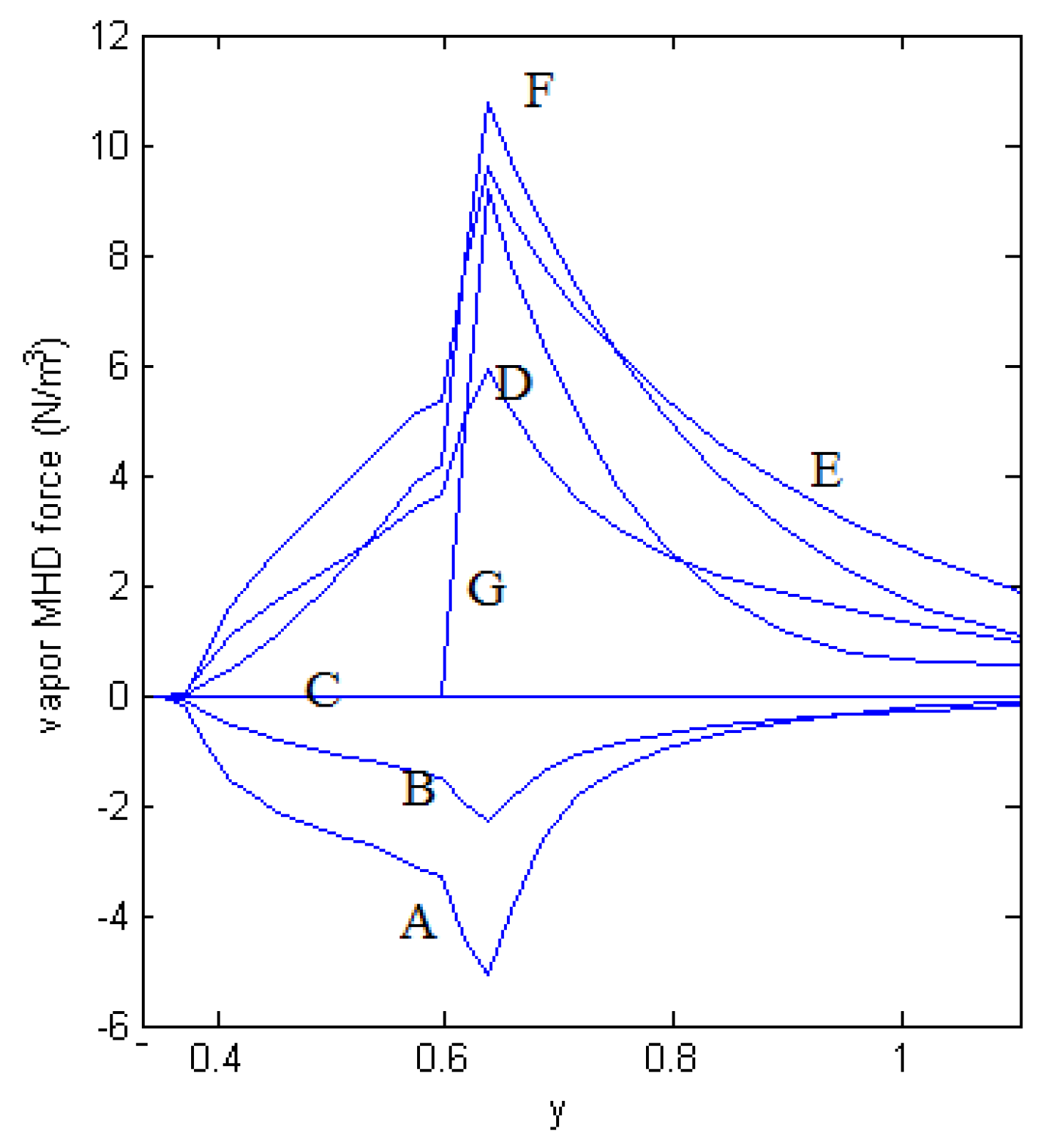
- Positive Lorentz force (in the flow direction) decreases and postpones the bubble generation.
- Negative Lorentz force (opposite of the flow direction) increases the bubble generation.
- Increasing of the positive Lorentz force increases the wall friction coefficient and wall friction force in both phases.
- By the increase of the electromagnetodynamic field, The net force on the fluid dramatically increased.
- Slip velocity changes such that it cannot be predicted by the previous relationships, and the new correlations for the slip velocity under MHD forces are presented (Equations (12)–(13)). The drift flux model is valuable only when the drift velocity is significant compared to the total volumetric flux. This limits its usefulness to the bubbly, slug and churn flow patterns.
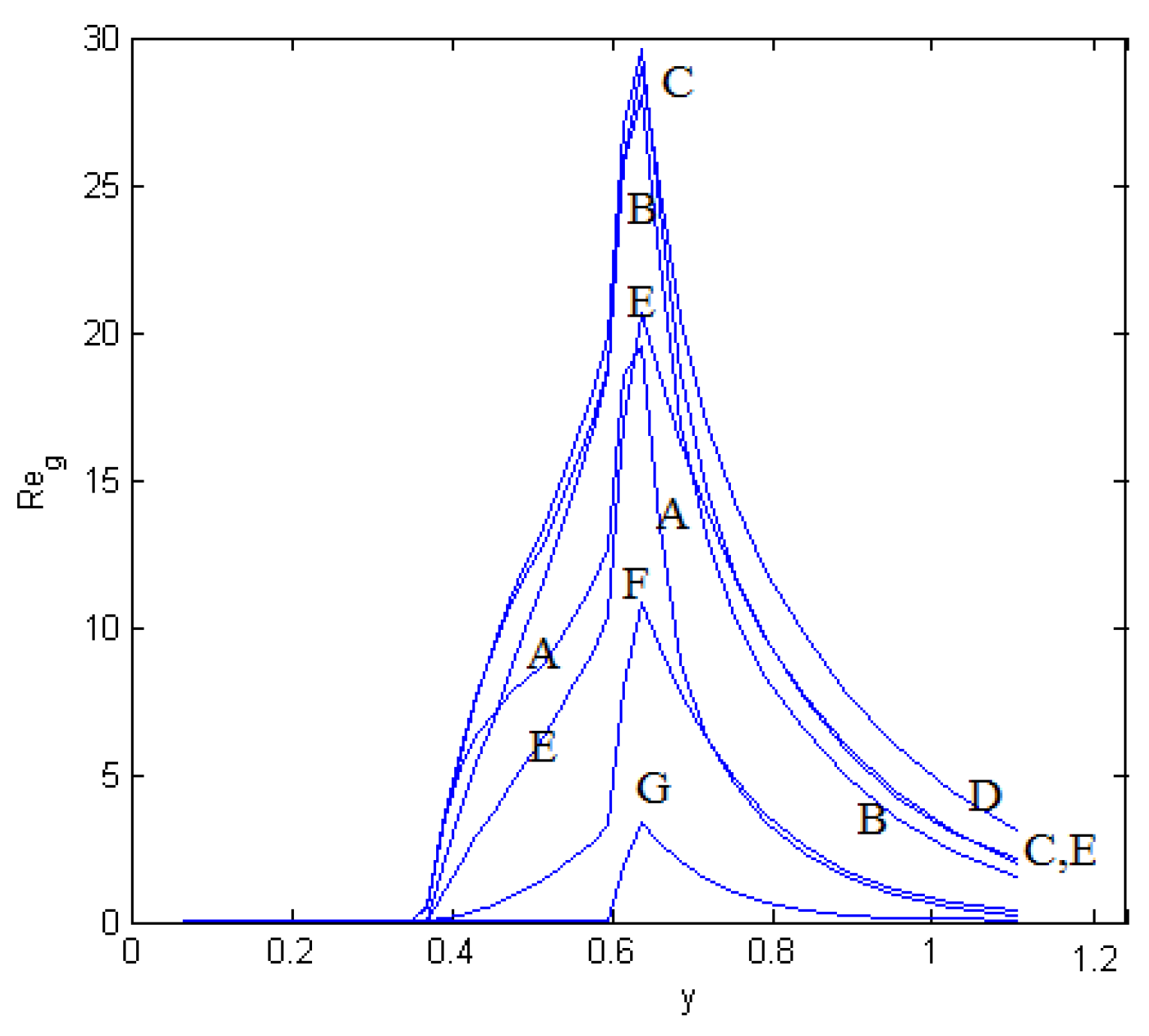
- The vapor phase Reynolds number decreases. This leads to diminishing of the velocity in the churn-turbulent region of bubbly flow.
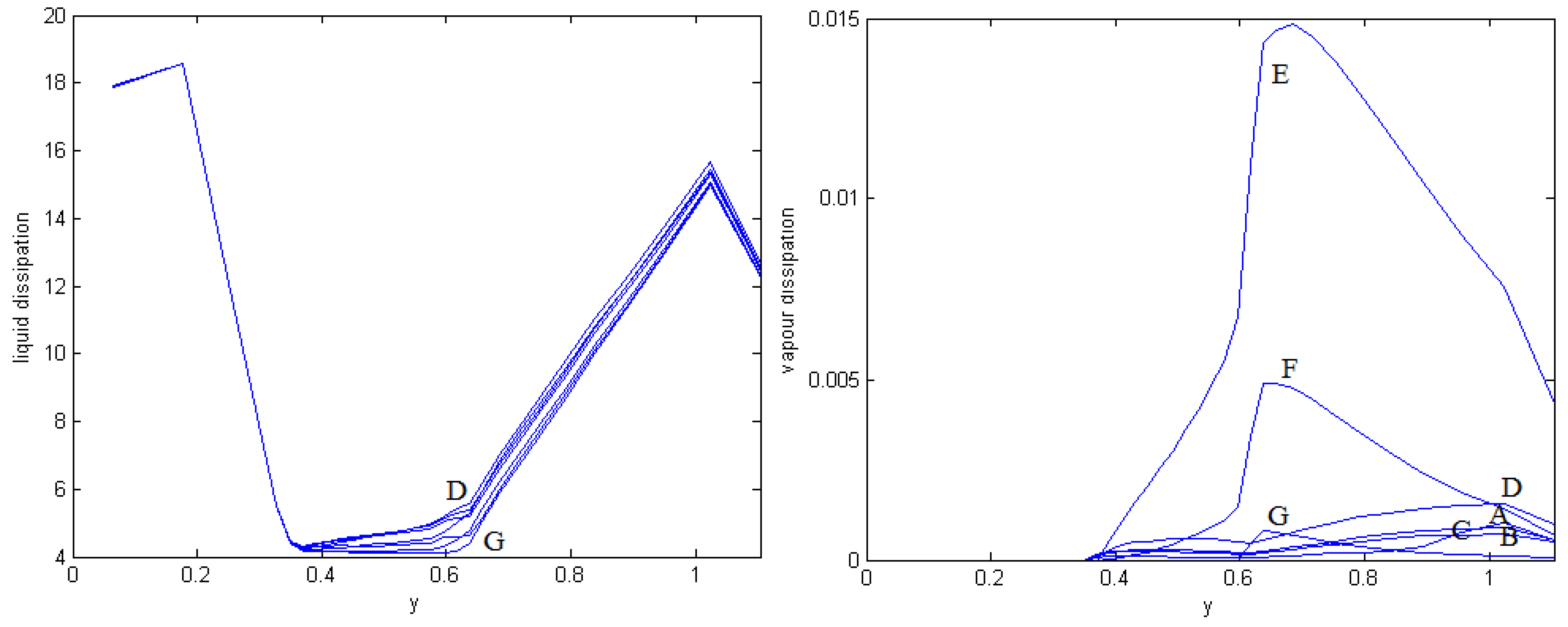
- By the increase of the electric and magnetic field, the vapor phase MHD force and, hence, the viscous dissipation in the fluid and liquid phases increases.
- By the increase of the liquid phase and postponement of the bubble generation, the density of the high absorbing medium increases, and the incident radiation and volumetric contribution of thermal radiation increases.
Author Contributions
Conflicts of Interest
Nomenclature
| A | area cross-section (m) |
| B | magnetic flux (T) |
| heat capacity, J/(kg·K) | |
| d | bubble diameter (m) |
| D | hydraulic diameter (m) |
| E | electric field, V/m |
| F | view factor |
| h | specific enthalpy (J/kg) |
| latent heat of evaporation (J) | |
| H | incident radiation (J/m s) |
| friction coefficient at wall | |
| f | bubble generation frequency (1/s) |
| g | gravitational acceleration (m/s) |
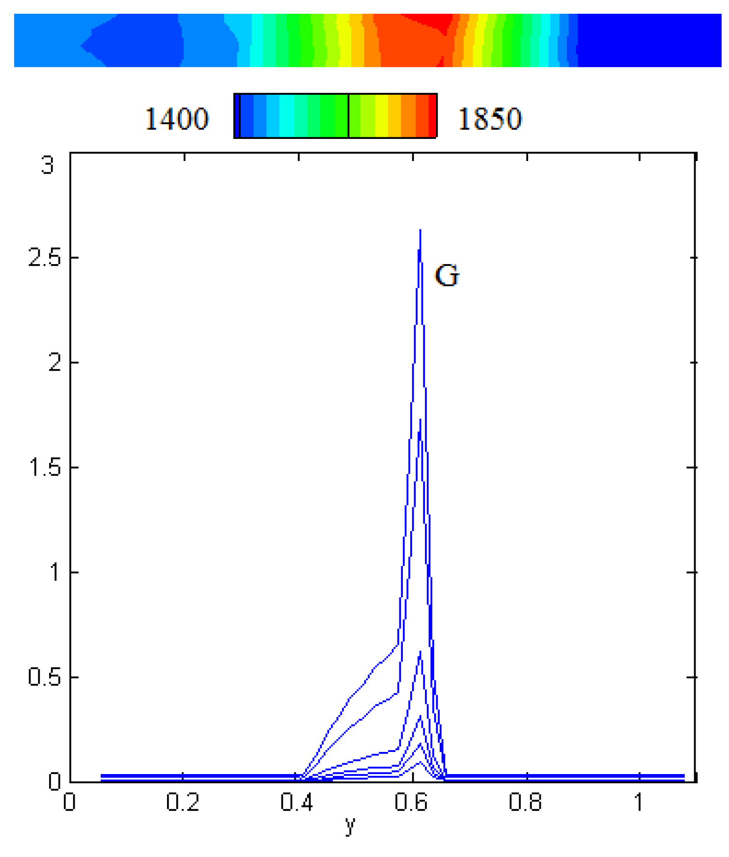
| G | mass velocity (kg/ms) |
| k | thermal conductivity (W/mK) |
| L | channel length (m) |
| m | mass flow rate (kg/s) |
| n | density of active nucleation sites |
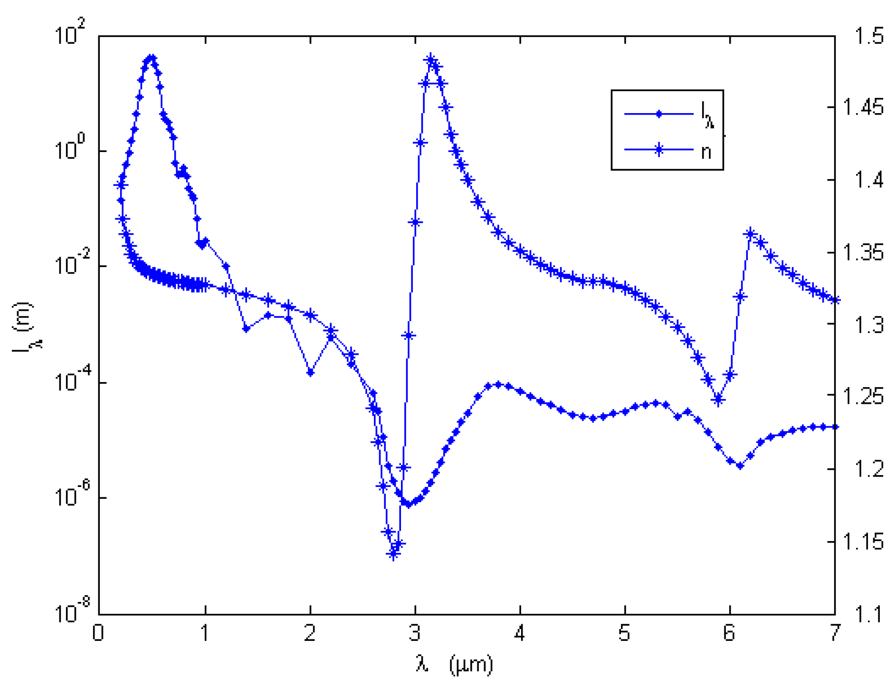
| index of refraction of water | |
| p | pressure (Pa) |
| radiation heat flu (J/ms) | |
| density of heat transfer at the wall (J/ms) | |
| S | slip velocity, (m/s) |
| T | temperature (K) |
| u | specific internal energy (J/kg) |
| v | velocity (m/s) |
| x | coordinate system along the magnetic field (m) |
| y | coordinate system along the tube (m) |
| z | coordinate system along the electric field (m) |
Greek symbols
| α | void fraction (m/s) |
| spectral absorption coefficient of water, = | |
| index of absorption of water | |
| ρ | fluid density (kg/m) |
| φ | electric potential (V) |
| μ | viscosity (kg/(s.m)) |
| Stefan-Boltzmann constant, =5.670373×10 (W·m·K) | |
| electric conductivity (S/m) | |
| surface tension (N/m) | |
| scattering coefficient (1/m) | |
| τ | wall shear stress (Pa) |
| ν | specific volume (m/kg) |
Superscript
| f | fluid phase |
| g | gas phase |
| max | maximum |
| min | minimum |
| r | radiation |
| sat | saturation |
| ∞ | ambient |
References
- Levy, S. Two-Phase Flow in Complex Systems; Wiley: New York, NY, USA, 1999. [Google Scholar]
- Joodaki, H.; Forman, J.; Forghani, A.; Overby, B.; Kent, R.; Crandall, J.; Beahlen, B.; Beebe, M.; Bostrom, O. Comparison of Kinematic Behaviour of a First Generation Obese Dummy and Obese PMHS in Frontal Sled Tests. In Proceedings of the 2015 IRCOBI Conference, Lyon, France, 9–11 September 2015; pp. 454–466.
- Foreman, J.; Joodaki, H.; Forghani, A.; Riley, P.; Bollapragada, V.; Lessley, D.; Overby, B.; Heltzel, S.; Kerrigan, J.; Crandall, J. Whole-body Response for Pedestrian Impact with a Generic Sedan Buck. Stapp Car Crash J. 2015, 59, 401–444. [Google Scholar]
- Forman, J.; Joodaki, H.; Forghani, A.; Riley, P.; Bollapragada, V.; Lessley, D.; Overby, B.; Heltzel, S.; Crandall, J. Biofidelity Corridors for Whole-Body Pedestrian Impact with a Generic Buck. In Proceedings of the 2015 IRCOBI Conference, Lyon, France, 9–11 September 2015; pp. 356–372.
- Yeoh, G.; Tu, J. Numerical modelling of bubbly flows with and without heat and mass transfer. Appl. Math. Modell. 2006, 30, 1067–1095. [Google Scholar] [CrossRef]
- Jamalabadi, M. Joule Heating in Low-Voltage Electroosmotic with Electrolyte containing nano-bubble mixtures through Microchannel Rectangular Orifice. Chem. Eng. Res. Des. 2015, 102, 407–415. [Google Scholar] [CrossRef]
- Roy, R.; Kang, S.; Zarate, J.; Laporta, A. Turbulent Subcooled Boiling Flow—Experiments and Simulations. ASME J. Heat Transfer 2002, 124, 72–93. [Google Scholar] [CrossRef]
- Makhmalbaf, M. Experimental study on convective heat transfer coefficient around a vertical hexagonal rod bundle. Heat Mass Transfer 2012, 48, 1023–1029. [Google Scholar] [CrossRef]
- Ghiaasiaan, S.M. Two-Phase Flow, Boiling, and Condensation: In Conventional and Miniature Systems; Cambridge University Press: Cambridge, UK, 2008. [Google Scholar]
- Lohrasbi, J.; Sahai, V. Magnetohydrodynamic heat transfer in two-phase flow between parallel plates. Appl. Sci. Res. 1988, 45, 53–66. [Google Scholar] [CrossRef]
- Jamalabadi, M.; Park, J. Electro-Magnetic Ship Propulsion Stability under Gusts. Int. J. Sci.: Basic Appl. Res. Sci. 2014, 14, 421–427. [Google Scholar]
- Makhmalbaf, M.; Liu, T.; Merati, P. Experimental Simulation of Buoyancy-Driven Vortical Flow in Jupiter Great Red Spot. In Proceedings of the 68th Annual Meeting of the APS Division of Fluid Dynamics, Boston, MA, USA, 22–24 November 2015.
- Malashetty, M.; Leela, V. Magnetohydrodynamic heat transfer in two phase flow. Int. J. Eng. Sci. 1992, 30, 371–377. [Google Scholar] [CrossRef]
- Branover, H. Liquid-metal MHD. In Proceedings of the 9th International Conference on Magnetohydrodynamic Power Generation, Tsukuba, Japan, 17–21 November 1986; pp. 1735–1749.
- Inoue, A.; Aritomi, M.; Takahash, M.; Narita, Y.; Yano, T.; Matsuzaki, M. Studies on MHD pressure drop and heat transfer of helium-lithium annular-mist flow in a transverse magnetic field. JSME Int. J. 1987, 30, 1768–1775. [Google Scholar] [CrossRef]
- Arosio, S.; Guilizzoni, M. Local Structure of Two-Phase Flows in Horizontal Ducts Effects of Uniform and Suddenly Varying Duct Sections. J. Vis. 2008, 11, 143–152. [Google Scholar] [CrossRef]
- Antal, S.; Lahey, R.; Flaherty, J. Analysis of phase distribution in fully developed laminar bubbly two-phase flow. Int. J. Multiph. Flow 1991, 17, 635–652. [Google Scholar] [CrossRef]
- Končar, B.; Kljenak, I.; Mavko, B. Modelling of local two-phase flow parameters in upward sub-cooled flow boiling at low pressure. Int. J. Heat Mass Transfer 2004, 47, 1499–1513. [Google Scholar]
- Chen, E.; Li, Y.; Cheng, X. CFD simulation of upward subcooled boiling flow of refrigerant-113 using the two-fluid model. Appl. Thermal Eng. 2009, 29, 2508–2517. [Google Scholar] [CrossRef]
- Shail, R. On laminar two-phase flows in magnetohydrodynamics. Int. J. Eng. Sci. 1973, 11, 1103–1108. [Google Scholar] [CrossRef]
- Moghaddam, S. Analytical solution of MHD micropump with circular channel. Int. J. Appl. Electromagn. Mech. 2012, 40, 309–322. [Google Scholar]
- Roman, C.; Dumont, M.; Letout, S.; Courtessole, C.; Vitry, S.; Rey, F.; Fautrelle, Y. Modeling of fully coupled MHD flows in annular linear induction pumps. Int. J. Appl. Electromagn. Mech. 2014, 44, 155–162. [Google Scholar]
- Jang, J.; Lee, S.S. Theoretical and experimental study of MHD (magnetohydrodynamic) micropump. Sens. Actuators A: Phys. 2000, 80, 84–89. [Google Scholar] [CrossRef]
- Malashetty, M.S.; Umavathi, J.C. Two-phase magnetohydrodynamic flow and heat transfer in an inclined channel. Int. J. Multiph. Flow 1997, 23, 545–560. [Google Scholar] [CrossRef]
- Cotton, J.; Robinson, A.; Shoukri, M.; Chang, J. A two-phase flow pattern map for annular channels under a DC applied voltage and the application to electrohydrodynamic convective boiling analysis. Int. J. Heat Mass Transfer 2005, 48, 5563–5579. [Google Scholar] [CrossRef]
- Sadek, H.; Robinson, A.; Cotton, J.; Ching, C.; Shoukri, M. Electrohydrodynamic enhancement of in-tube convective condensation heat transfer. Int. J. Heat Mass Transfer 2006, 49, 1647–1657. [Google Scholar] [CrossRef]
- Sadek, H.; Cotton, J.; Ching, C.; Shoukri, M. Effect of frequency on two-phase flow regimes under high-voltage AC electric fields. J. Electrostatics 2008, 66, 25–31. [Google Scholar] [CrossRef]
- Cotton, J.; Robinson, A.; Shoukri, M.; Chang, J. AC voltage induced electrohydrodynamic two-phase convective boiling heat transfer in horizontal annular channels. Exp. Thermal Fluid Sci. 2012, 41, 31–42. [Google Scholar] [CrossRef]
- Zeitoun, O.; Shoukri, M. Axial Void Fraction Profile in Low Pressure Subcooled Flow Boiling. Int. J. Heat Mass Transfer 1997, 40, 867–879. [Google Scholar] [CrossRef]
- Owen, R.G.; Hunt, J.C.R.; Collier, J.G. magnetohydrodynamic pressure drop in ducted two-phase flows. Int. J. Multiph. Flow 1976, 3, 23–33. [Google Scholar] [CrossRef]
- Serizawa, A.; Ida, T.; Takahashi, O.; Michiyoshi, I. MHD effect on nak-nitrogen two-phase flow and heat transfer in a vertical round tube. Int. J. Multiph. Flow 1990, 16, 761–788. [Google Scholar] [CrossRef]
- Collier, J.G.; Thome, J.R. Convective Boiling and Condensation, 3rd ed.; Oxford Engineering Science Series; Oxford Univercity Press: New York, NY, USA, 1996. [Google Scholar]
- Tu, J.Y. The influence of bubble size on void fraction distribution in sub-cooled flow boiling at low pressure. Int. Commun. Heat Mass Transfer 1999, 26, 607–616. [Google Scholar]
- Ranz, W.E.; Marshall, W.R. evaporation form drops. Chem. Eng. Prog. 1952, 48, 141–148. [Google Scholar]
- Shawkat, M.; Ching, C.; Shoukri, M. On the liquid turbulence energy spectra in two-phase bubbly flow in a large diameter vertical pipe. Int. J. Multiph. Flow 2007, 33, 330–316. [Google Scholar] [CrossRef]
- Shawkat, M.; Ching, C.; Shoukri, M. Bubble liquid turbulence characteristics of bubbly flow in a large diameter vertical pipe. Int. J. Multiph. Flow 2008, 34, 767–785. [Google Scholar] [CrossRef]
- Ransom, V.H. Course A-Numerical Modeling of Two-Phase Flows for Presentation at Ecole d’Ete d’Analyse Numerique; EGG-EAST-8546; Idaho National Engineering Laboratory: Idaho Falls, ID, USA, 1989. [Google Scholar]
- Tu, J.Y.; Yeoh, G.H.; Park, G.C.; Kim, M.O. On Population Balance Approach for Subcooled Boiling Flow Prediction. J. Heat Transfer 2005, 127, 253–264. [Google Scholar] [CrossRef]
- Mandhane, J.M.; Gregory, G.A.; Aziz, K. A Flow Pattern Map for Gas-Liquid Flow in Horizontal Pipes. Int. J. Multiph. Flow 1974, 1, 537–553. [Google Scholar] [CrossRef]
- Tu, J.Y.; Yeoh, G.H. On numerical modelling of low-pressure sub-cooled boiling flows. Int. J. Heat Mass Transfer 2002, 45, 1197–1209. [Google Scholar] [CrossRef]
- Peles, Y.; Haber, S. A steady state, one dimensional, model for boiling two phase flow in triangular micro-channel. Int. J. Multiph. Flow 2000, 26, 1095–1115. [Google Scholar] [CrossRef]
- Jamalabadi, M. MD Simulation of Brownian Motion of Buckminsterfullerene Trapping in nano-Optical Tweezers. Int. J. Opt. Appl. 2015, 5, 161–167. [Google Scholar]
- Jamalabadi, M. Entropy generation in boundary layer flow of a micro polar fluid over a stretching sheet embedded in a highly absorbing medium. Front. Heat Mass Transfer 2015, 6, 1–13. [Google Scholar]
- Jamalabadi, M. Numerical Investigation of Thermal Radiation Effects on Electrochemical Impedance Spectroscopy of a Solid Oxide Fuel Cell Anodes. Mater. Perform. Charact. 2015, 4, 1–28. [Google Scholar]
- Modest, M. Radiative Heat Transfer; Academic Press: San Diego, CA, USA, 2003. [Google Scholar]
- Reed, W.; Stewart, H.B.; Wolf, L. Applications of the THERMIT code to 3D Thermal Hydraulic Analysis of LWR Cores. In Proceeding of top meeting on Computational methods in nuclear engineering, Williamsburg, VA, USA, 23–25 April 1979. BNL-25484.
- Zolotarev, V.; Demin, A. Optical properties of water in the wide wavelength range 0.1A 1 m. Opt. Spectrosc. 1977, 43, 271–279. [Google Scholar]
- Hale, G.; Querry, M. Optical constants of water in the 200 nm to 200 lm wavelength region. Appl. Opt. 1973, 12, 555–563. [Google Scholar] [CrossRef] [PubMed]
- Mobley, C.D.; Rudolph, W.P. Light and Water: Radiative Transfer in Natural Water; Academic Press: San Diego, CA, USA, 1994. [Google Scholar]
- Pope, R.M.; Fry, E.S. Absorption spectrum (380–700 nm) of pure water. II. Integrating cavity measurements. Appl. Opt. 1977, 36, 8710–8723. [Google Scholar] [CrossRef]
- Dombrovsky, L. Large-cell model of radiation heat transfer in multiphase flows typical for fuel–coolant interaction. Int. J. Heat Mass Transfer 2007, 50, 3401–3410. [Google Scholar] [CrossRef]
- Lu, X.; Wang, T. Investigation of radiation models in entrained-flow coal gasification simulation. Int. J. Heat Mass Transfer 2013, 67, 377–392. [Google Scholar] [CrossRef]
- Wallis, G.B. One-Dimensional Two-Phase Flow; McGraw-Hill: New York, NY, USA, 1969. [Google Scholar]
- Zuber, N. The dynamics of vapor bubbles in nonuniform temperature fields. Int. J. Heat Mass Transfer 1961, 2, 83–98. [Google Scholar] [CrossRef]


| () | (T) | Case |
|---|---|---|
| A | 0.1 | |
| B | 0.1 | |
| C | 0 | 0 |
| D | 1 | 0.2 |
| E | 2.5 | 0.25 |
| F | 5 | 0.3 |
| G | 10 | 0.45 |
© 2016 by the authors; licensee MDPI, Basel, Switzerland. This article is an open access article distributed under the terms and conditions of the Creative Commons Attribution (CC-BY) license (http://creativecommons.org/licenses/by/4.0/).
Share and Cite
Mirzaee, M.; Hooshmand, P.; Ahmadi, H.; Balotaki, H.K.; KhakRah, H.; Abdollahzadeh Jamalabadi, M.Y. Electromagnetohydrodynamic Effects on Steam Bubble Formation in Vertical Heated Upward Flow. Energies 2016, 9, 657. https://doi.org/10.3390/en9080657
Mirzaee M, Hooshmand P, Ahmadi H, Balotaki HK, KhakRah H, Abdollahzadeh Jamalabadi MY. Electromagnetohydrodynamic Effects on Steam Bubble Formation in Vertical Heated Upward Flow. Energies. 2016; 9(8):657. https://doi.org/10.3390/en9080657
Chicago/Turabian StyleMirzaee, Mojtaba, Payam Hooshmand, Hamed Ahmadi, Hassan Kavoosi Balotaki, HamidReza KhakRah, and Mohammad Yaghoub Abdollahzadeh Jamalabadi. 2016. "Electromagnetohydrodynamic Effects on Steam Bubble Formation in Vertical Heated Upward Flow" Energies 9, no. 8: 657. https://doi.org/10.3390/en9080657
APA StyleMirzaee, M., Hooshmand, P., Ahmadi, H., Balotaki, H. K., KhakRah, H., & Abdollahzadeh Jamalabadi, M. Y. (2016). Electromagnetohydrodynamic Effects on Steam Bubble Formation in Vertical Heated Upward Flow. Energies, 9(8), 657. https://doi.org/10.3390/en9080657