MMCS: Multi-Module Charging Strategy for Increasing the Lifetime of Wireless Rechargeable Sensor Networks

Abstract

In recent years, wireless charging technology has provided an alternative to charging equipment. Wireless charging technology has already proved to be useful in our daily lives in phones, buses, restaurants, etc. Wireless charging technology can also be applied in energy-bounded wireless sensor networks (WSNs), and these are called wireless rechargeable sensor networks (WRSNs). The optimized charging path problem is the most widely discussed issue in employing WRSNs with wireless charging vehicles (WCVs). This problem involves determining the most efficient path for charging sensor nodes. Further, charging-scheduling problems also need to be considered in the optimized charging path problem. In this paper, we proposed a multi-module charging strategy (MMCS) used to prolong the lifetime of the entire WRSN. MMCS can be divided into three stages: the charging topology, charging scheduling, and charging strategy stages, with multiple modules in each stage. The best module combination of MMCS is the distance-based module in the charging topology stage, delay-based module in the charging schedule stage, and the average lifetime module in the charging strategy stage. The best module combination enables prolonging the lifetime efficiently, as it considers not only the priority of urgent nodes but also the travel distance of WCV; the delay-based module of the charging schedule stage considers the delay effect on the follow-up nodes. The experimental results show that the proposed MMCS can improve the lifetime of the entire WRSN and that it substantially outperforms the nearest job next with preemption (NJNP) method in terms of lifetime improvement of the entire WRSN.

1. Introduction

As the maturity of wireless charging technology increased, researchers began using wireless charging for wireless sensor networks (WSNs), resulting in implementations defined as wireless rechargeable sensor networks (WRSNs). WSNs are becoming more and more popular, from indoor applications to the monitoring of environmental pollution. Because the features of the WSNs contribute to high node replacement costs, the deployed sensor nodes are not changed after deployment. One reason for this is the multitude of deployed sensor nodes in WSNs. Additionally, WSNs are often deployed in inaccessible areas in order to remotely monitor the special environment. Replacing large numbers of the sensor nodes or replacing nodes in remote areas therefore drives the high replacement costs.

However, these sensor nodes are limited by battery. Some of these sensor nodes may serve as an important packet transmission route, leading to higher energy consumption due to increased usage of the node. These sensor nodes that serve as key components will therefore exhaust their energy supply earlier, impacting availability in WSNs by causing a gap in sensing capability or even collapse of the WSN. These issues cause inaccurate sensing results or unacceptably reduce the precision of recovery information.

These dead sensor nodes with depleted energy sources can be rescued manually, but manual intervention incurs enormous costs. Therefore, follow-up studies have examined other methods to extend the lifetime of WSNs. The first method reduces the energy consumption of network nodes. For example, the cluster algorithm reduces the loading of the sensor nodes by using clusters to centralize packet transfers. The other method uses extra energy harvested from the environment, such as the use of solar energy to supply power to the sensor nodes.

Wireless charging technology is an effective solution to extend the lifetime of WSNs. Wireless charging technology can utilize a mobile wireless charging vehicle (WCV) to rescue the dying nodes by supplementing their remaining energy. However, the wireless charging technology in the WSNs is facing several challenges. Since the sensor nodes are randomly distributed in the ground, the WCV must determine an appropriate travel path to charge the sensor nodes. Since these sensor nodes perform different workloads, they exhibit differing energy consumption profiles over time. This necessitates the determination of a charging priority for some sensor nodes based on the expected death order. Thus, this paper proposed an algorithm that accounts for charging order as well as the WCV travel path.

2. Related Works

In recent years, wireless power transfer (WPT) has been widely used in WSNs. WCVs were introduced to periodically charge the batteries in the sensors, thereby extending the lifecycles of WSNs [1]. WCV-related issues are examined in a large number of studies. The most important issue involves the determination of the charging schedule, such that each sensor node receives an appropriate charge to maximize the lifecycle of the WSN.

Xie et al. [2] first defined the application of WPT technology to WSNs. As shown in Figure 1, the authors identify the WCV in WSNs as periodically patrolling and charging each sensor node. Each cycle is divided into two stages. The first stage represents the WCV patrol service. The WCV charges all sensor nodes and gathers information during this stage. In the second stage, the WCV returns to its service station and idles until the next patrol service begins.

To ensure that each sensor node can be promptly charged, Xie et al. [2] propose a new concept of the renewable energy cycle and define the necessary and sufficient conditions for the case. Once all conditions are met, their method can provide a renewable energy cycle, so that the WSNs’ lifecycles are extended indefinitely. They further study the period optimization problem that aims to maximize the ratio of time spent during the idle stage in the service station to the duration of the patrol cycle, thereby achieving the most efficient patrol-charging mode. For this problem, they demonstrated that the optimal route is the shortest Hamiltonian cycle.

Although Xie et al. [2] proposed a sustainable WSN deployment environment, the solution exhibits a major drawback in its lack of scalability. It must meet all the specified conditions for the use of the method proposed by Xie et al. Once a WSN’s sensor node density increases, the issue of how to use WPT technology to extend the lifecycle of WSNs must still be effectively addressed. Kurs et al. [3] also defined WRSN scalability issues and proposed the development of an enhanced magnetic resonance coupling technology that allows more than one WCV to charge the sensor nodes at the same time. Xie et al. [4,5,6,7] adopt the concept Kurs et al. [3] proposed to improve the method for applying WPT in high-density WSNs. Xie et al. [2] believe the WCV will follow the same two-stage cycle. The WCV starts from the service station and travels throughout the WSN to charge sensor nodes, and then returns to idle in the service station until the next cycle begins. Differing from Xie et al. [2], the WCV can simultaneously charge the sensor nodes that are located within the energy transmission range. Based on the energy transmission range of the WCV, Xie et al. [4,5,6,7] proposed a hexagonal cell, similar to cellular networks, and selected the best rechargeable point within those hexagonal cells, as in Figure 2. Based on the general power charging mode, they combined the cycle optimization problem with the path planning optimization problem. For this issue, they provide a method to determine the optimal solution.

In addition to Xie et al., there are many scholars researching the field of wireless charging. Guo et al. [8] studied the issue of combining simultaneous wireless charging with mobile data collection in WRSNs, with a goal of maximizing the efficiency of the WSN using the WCV. Fu et al. [9] presented an optimized travel strategy that finds the best location for multi-charging situations and proved that this method has low complexity. The above methods are mostly focused on providing WCV travel path optimization and aim to provide efficiency during charging. However, the above-mentioned methods do not account for differing energy consumption between sensor nodes. Different energy consumption rates arise due to the differing importance of sensor nodes, and thus different data generation rates.

Hu et al. [10] considered the effect of the imbalance between WRSN sensor node energy consumption and proposed an on-demand mobile charging planning and deployment method for the service station. The goal of the approach is to minimize the total energy consumption of the WCV. On-demand charging problems are always defined as scheduling issues. The most intuitive and easiest scheduling solution is first-come, first-served (FCFS), whose effectiveness has been extensively studied in queueing theory [11]. However, scheduling a FCFS system is based on the order of the request time. Regarding spatial traversal of the WSN, FCFS would lead the WCV back and forth repeatedly to already-visited sensor nodes [12]. He et al. [13,14] observe the contrast of FCFS to an on-demand mobile charging theory. He et al. [13,14] proposed the concept of nearest job next with preemption (NJNP), which is based on FCFS. Although NJNP can take account of both the request time and spatial characteristics to move and charge sensor nodes, NJNP does not ensure the survival of the sensor nodes by prioritizing sensor nodes with higher energy exhaustion probability. Also, He et al. do not consider the capacity of the battery of the WCV.

As shown in

Table 1. Comparison of the recent developments in wireless rechargeable sensor network (WRSN).

Reference	Focus on	Energy Constraints of WCV 1	Traveling Path (Static/Dynamic)
Guo et al. (2013) [8]	Traveling path of WCV	No	Static
Fu et al. (2013) [9]	Traveling path of WCV	No	Static
Hu et al. (2013) [10]	On-demand mobile charging problem (scheduling)	No	Dynamic
Xie et al. (2012–2015) [4,5,6,7]	Traveling path of WCV	No	Static
He et al. (2013–2015) [13,14]	On-demand mobile charging problem (scheduling)	No	Dynamic

¹: The energy constraints of WCV is considered in this work.

, most recent WRSN research focuses on path optimization and scheduling issues, but WRSN solutions based on the optimized travel path problem are mostly static-path solutions. These proposals did not take into account the different power consumption rates due to the differing importance of sensor nodes, resulting in the failure of the sensor nodes to effectively charge. Although the algorithms based on on-demand charging can provide dynamic travel path planning, such algorithms assume the WCV has sufficient energy. In real world applications, WCV power is limited by the size of the battery, thereby affecting the path planning and scheduling. Current multi-charging technology is affected by the energy transmission distance and produces unnecessary energy consumption of from the WCV. Therefore, this paper used a single-point charging technology to reduce energy waste and proposed a dynamic algorithm designed to improve energy allocation efficiency to maximize the lifecycles of WSNs.

This paper also surveyed for existing wireless charging technology, as shown in

Table 2. Comparisons between wireless charging technologies.

Type	Electromagnetic Induction	Coupling Magnetic Resonance	Micro-Wave Conversion	Laser Light Sensor
Theory	Faraday‘s law	Same resonance frequency energy transfer	Electromagnetic wave transfer	Laser and the Solar panels
Power transmission	W~hundreds of KW	W~hundreds of KW	>100 mW	hundreds of KW
Transmission distance	<10 cm	5 m	>10 m	>100 m
Conversion efficiency	70%	50%	1.6%	25%
Advantage	High conversion efficiency	Multiple charging	Radio wave transmission and automatic charging anywhere	Technology matures over long distances

. As electromagnetic inductive (EI) charging technology has high efficiency, it can reduce the charging time for extending the life cycle of WSNs in the least amount of time. Therefore, we chose EI in our simulations. However, EI has a limited charging distance. Therefore, we designed an efficient charging path through which WCV reaches each low-power sensor in the shortest time.

3. Multi-Module Charging Strategy

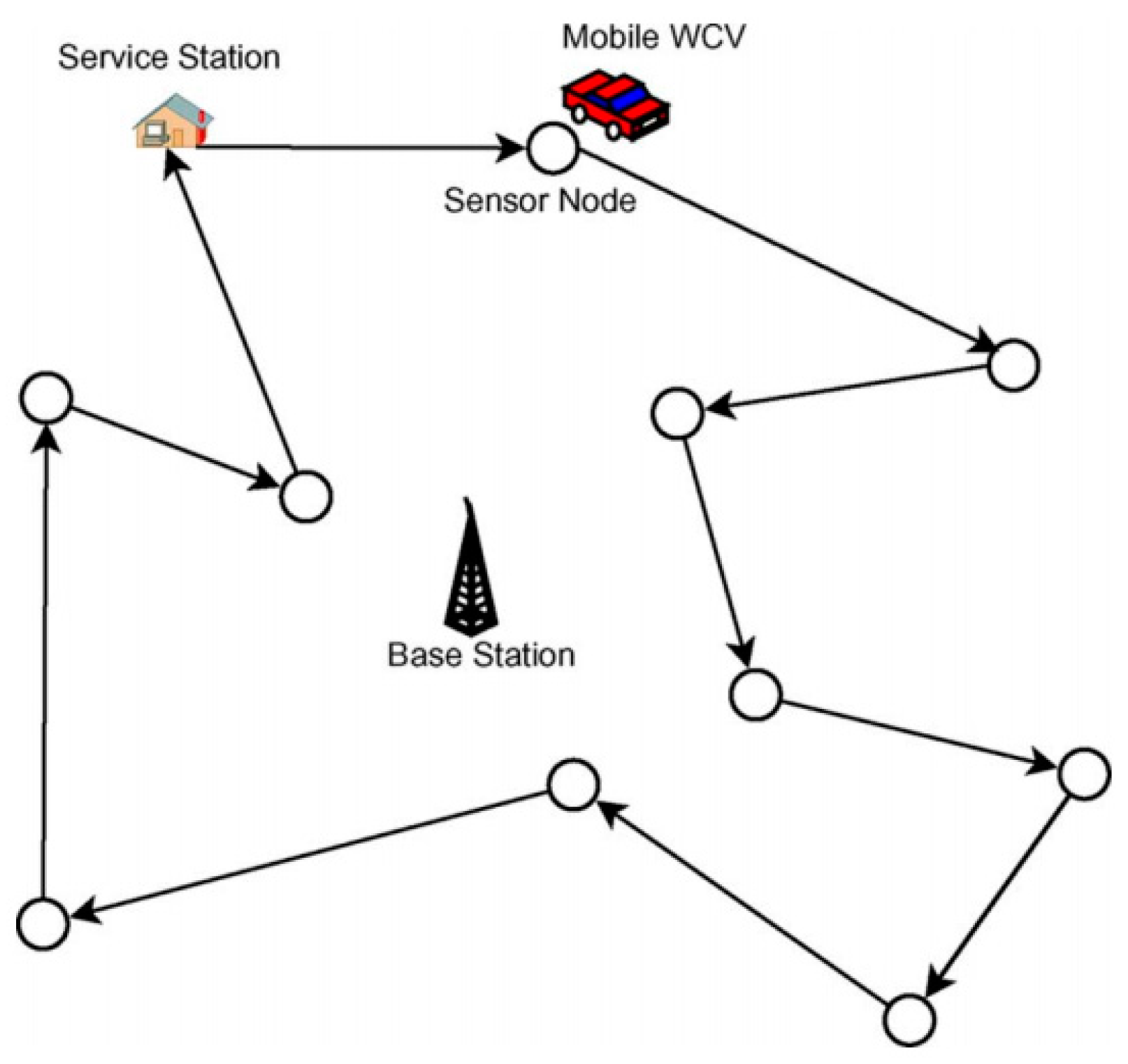
3.1. Problem Definition

The optimized charging path problem is the most widely discussed issue in employing WCV in WRSNs. This problem involves determining the most efficient path for charging sensor nodes. Further, charging-scheduling problems also need to be considered in the optimized charging path problem. A key point of the optimized charging path problem is scheduling the charging order of sensor nodes without any dead nodes. Thus, in this study, we integrate the optimized charging path problem and the charging-scheduling problem. Further, we considered the energy constrains of WCV and proposed a dynamic path planning method to extend the lifetime of WRSNs.

This study adopts the sensor nodes are randomly deployment in the given area, as shown in Figure 3. A base station is not only the starting point for WCVs, but also the place for replacing the WCV’s battery. The base station is a data sink located at the central of the WRSNs. The parameter definitions of the sensor nodes and WCVs are listed in

Table 3. The definition of related parameters.

Parameter	The Definition of Parameter
BS	Base station
N	Set of all sensor nodes
CNs	Candidate nodes are the set of nodes selected for charging, $CNs\in N$
En	Energy of sensor node n. $n\in \text{integer}$
Cn	Energy consumption for sensor node n
LTn	Rest of the lifetime of sensor node n
EDn	Energy demand of sensor node n
Bm	Battery for WCV moving
Bc	Battery for WCV charging sensor nodes
V	Travelling speed of WCV
CM	Energy consumption of WCV
R	Charging rate of the sensor nodes
Di,j	Path distance of Nodei to Nodej
Tt	Total travelling time of WCV
CG	Consumption grades of sensor nodes
CDik	Cumulative total travel time of WCV from Nodei to Nodek
CEDik	Cumulative total time of charging the noden from Nodei to Nodek
DTik	Delay time of Nodek

.

In WRSNs, all sensor nodes have the same battery capacity; however, they have different energy consumptions for different workloads. Therefore, each sensor Node_n can use Equation (1) to calculate LT_n:

$$L{T}_n=\frac{E_n}{C_n}$$

(1)

This paper discusses the optimized charging path problem with one WCV to rescue the Node_n in WRSNs. Each WCV has two independent batteries: One for moving the vehicle and the other for charging Node_n. When WRSNs run for a while, Node_n needs to be charged. The optimized charging path problem is to improve total lifetime of WRSNs. In addition, there is the problem of how to select urgent nodes as candidate nodes CNs, and charge the CNs efficiently to prolong the lifetime of WRSNs.

In order to simplify the calculation of the charging scheduling problem, the calculation transformed the distance into time. D_i,j represents the distance between the source Node_i and the destination Node_j, and $\frac{D_{i,j}}{V}$ represents WCV’s travel time without the time for charging. ED_n represents the energy demand for noden. The travel time considering the time for charging Node_n represents the total travelling time of WCV, as shown in Equation (2):

$$T_{\mathrm{t}}=\frac{D_{i,j}}{V}+\frac{{\displaystyle {\sum }_{n\in CNs}E{D}_n}}{R},\text{ that }CNs\in N,i\ne j$$

(2)

Path planning and charging scheduling are subject to the restrictions in both battery power B_c and B_m of WCV, and it seeks to minimize T_t and as well as maximize the life time of the WRSNs, as shown in Equations (3) and (4):

$$\text{Min }{T}_{\mathrm{t}}=\frac{D_{i,j}}{V}+\frac{{\displaystyle {\sum }_{n\in CNs}E{D}_n}}{R},\text{ that }CNs\in N,i\ne j$$

(3)

$$\text{Max }{\displaystyle {\sum }_{n\in CNs}\frac{E_n+E{D}_n}{C_n}}$$

(4)

The battery capacity constraints of WCV are:

$$BC\ge {\displaystyle {\sum }_{n\in CN}E{D}_n}$$

(5)

$$BM\ge T_{\mathrm{t}}\times C_M$$

(6)

3.2. Method Description

This paper proposes multi-module charging strategy (MMCS) based on the Dijkstra algorithm, which is used for finding the shortest paths between nodes in a graph. MMCS defined the charging topology between nodes based on distance, energy, and lifetime. Owing to the two constraints of the WCV’s battery capacity, WCV cannot charge all sensor nodes at the same time. Furthermore, MMCS proposes two different charging scheduling methods. In addition, in order to prolong the lifetime of the entire WRSNs, MMCS is designed such that the two charging strategies improve energy consumption and lifetime of the WRSNs. MMCS can be divided into three stages, as shown in the Figure 4: the charging topology, charging scheduling, and charging strategy stages, with multiple modules in each stage: the charging topology stage defines the charging scope and constructs the charging topology; the charging scheduling stage selects the Node_n for charging; MMCS has designed two charging scheduling methods based on Dijkstra; and the charging strategy stage is used to calculate the energy demand ED_n of Node_n. The details of all three stages are introduced in this section, and the simulated results are presented in Section 4.

3.2.1. The Stage of Charging Topology

The charging topology stage is used to select candidate nodes CNs that will be scheduled to charge in the travel path. To improve the energy level of low-energy nodes, the CNs are chosen according to their LT_n. However, WCV’s power is limited by the size of its battery; therefore, MMCS was used to design three methods to construct the topology and plan a travel path with reduced cost.

Definition of charging scope: MMCS utilizes the Expectations E(N) to define the number of candidate nodes |CNs|; |N| represents the number of nodes. Owing to the energy consumption of nodes are randomized, each Node_n is categorized into an energy consumption grade (CG). The number of nodes in each CG could be estimated by $E\left(N\right)=\left|N\right|\times \frac{1}{CG}$. Obviously, the first grade consists of death nodes with the highest energy consumption. However, the second grade must also be considered. Therefore, in the MMCS, $\left|CNs\right|=E\left(N\right)\times 2$ is defined to be the number of candidate charging nodes, indicating that MMCS selects $\left|CNs\right|$ nodes with lowest LT_n as CNs.

Topology construction: The topology is constructed according to three aspects (distance, energy and lifetime) to establish three modules:

• Distance-based module: The travel distance of a WCV is limited by its battery capacity. In MMCS, a distance-based topology is designed to plan the shortest travel path. The first node S is the ${\text{Node}}_{n\in CNs}$ with the lowest LT_n. Node S then establishes adjacent relations with three ${\text{Node}}_{n\in CNs}$ with the shortest distance to S. The next node is the ${\text{Node}}_{n\in CNs}$ with the shortest path to S. Repeat this process until all the CNs are complete.
• Energy/Lifetime-based module: The energy consumption rate of each ${\text{Node}}_{n\in CNs}$ is different; however, there are different degrees of criticality. Therefore, MMCS utilizes the remainder of energy/lifetime as a basis for establishing the topology. In terms of energy-based topology construction, each ${\text{Node}}_{n\in CNs}$ is first sorted in the ascending order, then the ${\text{Node}}_{n\in CNs}$ is sequentially chosen as Node S, which establishes adjacent relations with three ${\text{Node}}_{n\in CNs}$ with the lowest E_n. In lifetime-based construction, ${\text{Node}}_{n\in CNs}$ is selected because of its lifetime.

3.2.2. The Stage of Charging Scheduling

The ${\text{Node}}_{n\in CNs}$ with the lowest remaining lifetime should be the node the most in need to be rescued. Owing to the random deployment of sensor nodes, only considering the lifetime may exhaust B_m in one round trip. We believe that the energy consumption due to repeated movements could be reduced if the WCV is able to rescue other CNs on the path to the nodes with the lowest lifetime. Therefore, the MMCS based on the Dijkstra algorithm proposed the best-effort and delay-based modules:

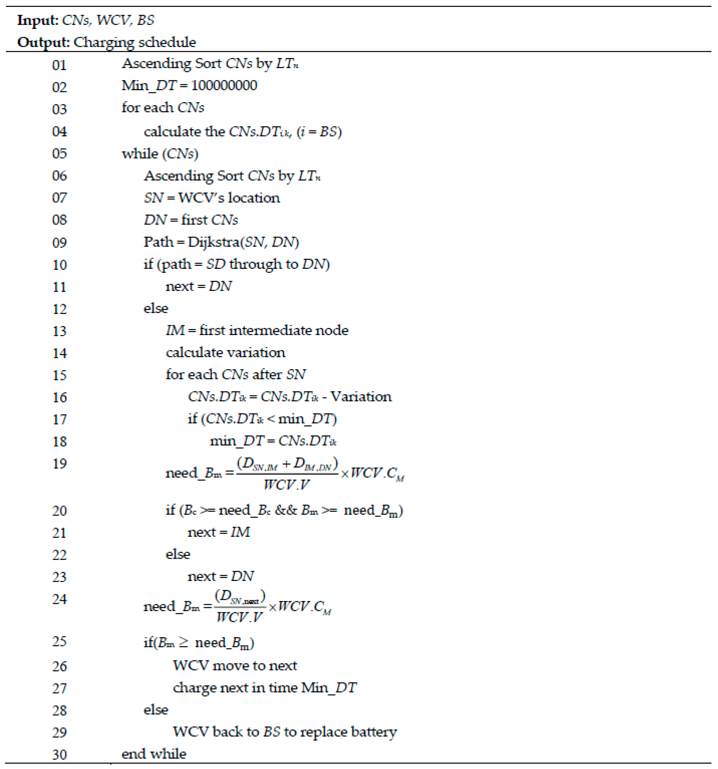
• Best-effort module: Best effort is a concept used for attempting the rescue of ${\text{Node}}_{n\in CNs}$ which WCV can pass. The best-effort module algorithm is shown in Figure 5. The nodes in ${\text{Node}}_{n\in CNs}$ are first sorted in an ascending order; then, MMCS is used to define the source (SN) as the present location of WCV and its destination (DN) as the location of ${\text{Node}}_{n\in CNs}$ with lowest LT_n. Next, the Dijkstra algorithm is executed to determine the shortest path. If SN does not directly connect with the DN, check if B_c and B_m are sufficient to charge and move to the first relay ${\text{Node}}_{n\in CNs}$ between SN and DN, and then from first relay ${\text{Node}}_{n\in CNs}$ to DN. If energy is sufficient, the first relay ${\text{Node}}_{n\in CNs}$ is defined as the next node to which WCV will move to charge.
• Delay-based module: The concept of best effort only considers the relay station bringing the result of DN. However, the insert relay ${\text{Node}}_{n\in CNs}$ not only affect the DN but also other ${\text{Node}}_{n\in CNs}$ that are subsequent to SN. If a ${\text{Node}}_{n\in CNs}$ subsequent to SN is more critical than relay ${\text{Node}}_{n\in CNs}$, it may lead to node death. Therefore, in the MMCS the delay time is considered instead of the scheduling time, and the delay-based method is proposed. Figure 6 shows the process of delay time.

The ${\text{Node}}_{n\in CNs}$ nodes are first sorted in an ascending order. Next, by using MMCS, source SN is defined as present location of WCV and destination DN is the location of ${\text{Node}}_{n\in CNs}$ with lowest LT_n. The Dijkstra algorithm is then executed to determine the shortest path. Equation (7) is used to calculate the delay time DT_ik of CNs that are scheduled by ascending values of LT_k, which reduces the time spent on travelling to Node_k. DT_ik implies the time that can be delayed for reaching Node_k. The cumulative total travel time CD_ik is defined by Equation (8), and cumulative total energy demand of sensor nodes CED_ik is shown in Equation (9):

$$D{T}_{ik}=L{T}_k-C{D}_{ik}-CE{D}_{ik}$$

(7)

$$C{D}_{ik}=\frac{D_{ik}}{V}$$

(8)

$$CE{D}_{ik}=\frac{{\displaystyle {\sum }_{n\in N_{ik}}E{D}_n}}{R},\text{ that }{N}_{ik}\in N,i\ne k$$

(9)

If SN does not directly connect DN, check whether B_c and B_m are sufficient to charge and move to first relay ${\text{Node}}_{n\in CNs}$ between SN and DN, and from first relay ${\text{Node}}_{n\in CNs}$ to DN. If the energy is sufficient, it is confirmed that no more death nodes are caused by the insert relay ${\text{Node}}_{n\in CNs}$ in the schedule. If there are no dead ${\text{Node}}_{n\in CNs}$, relay ${\text{Node}}_{n\in CNs}$ is defined as the next node that the WCV will move to. Next, the values of LT_n are then updated and resorted after charging ${\text{Node}}_{n\in CNs}$.

In the charging process, Equation (10) can be used to verify whether the relay node has resulted in a death node. Figure 7 shows the process of scheduling, which is represented by a solid line LT_i (Node_i → Node_x → Node_x+1 → Node_x+2 → Node_y → Node_j). Further, the dotted line represents the process for inserting Node_y between Node_i and Node_x (Node_i → Node_y → Node_x → Node_x+1 → Node_x+2 → Node_j). Changing the schedule would mean ${\text{Node}}_{n\in CNs}$ is divided into three cases. In Case 1, ${\text{Node}}_{n\in CNs}$ is scheduled before Node_x. Owing to these nodes being charged, they are not affected by the relay node. In Case 2, ${\text{Node}}_{n\in CNs}$ is scheduled after Node_y. The DT_ik of these nodes are affected by the changing schedule. The change in schedule causes distance variation. However, Node_y represents the relay node, and charging Node_y on the way from Node_i to Node_x can reduce energy consumption. Therefore, when Node_y becomes the relay node, it does not result in an extra death node. In Case 3, ${\text{Node}}_{n\in CNs}$ is scheduled between Node_x and Node_y. The DT_ik of these nodes are affected by the changing schedule. The distance variation can be calculated using Equation (10). If any DT_ik of nodes in Case 3 are shorter than the variation, Node_y would cause a death node. As shown in Equation (11), Node_y is not the most critical node; therefore, the maximum charging time is the minimum delayable time of ${\text{Node}}_{n\in CNs}$ in Case 3.

$$Variation(\mathsf{\tau })=\frac{D_{iy}+D_{yx}-D_{ix}}{v}$$

(10)

$$\text{Min }\{D{T}_{i,2}-\mathsf{\tau },D{T}_{i,3}-\mathsf{\tau },D{T}_{i,4}-\mathsf{\tau },\dots D{T}_{i,k-1}-\mathsf{\tau }\}$$

(11)

3.2.3. The Stage of Charging Strategy

The charging strategy stage is used to define ED_n of each node. The MMCS considers E_n and LT_n to develop two charging modules: average energy and average lifetime, respectively.

• Average energy module: As shown in Equation (12), CNs selected in the charging topology stage are nodes that are more urgent. To enhance CNs to a high-energy level, MMCS uses double CNs (dCNs) as threshold for improving energy. Next, the E_n of urgent nodes is enhanced by enhancing energy of nodes with the lowest E_n to next higher energy level.

  $$E{D}_n=\frac{{\displaystyle {\sum }_{n\in dCNs}{E}_n}}{\left|dCNs\right|}-E_i$$

  (12)
• Average lifetime module: As shown in Equation (13), to enhance CNs to a high-energy level, MMCS uses dCNs as threshold for improving energy. The LT_n of critical nodes is enhanced by enhancing the energy of nodes with the lowest LT_n to next higher lifetime level.

  $$L{T}_n=\left(\frac{{\displaystyle {\sum }_{n\in dCNs}L{T}_n}}{\left|dCNs\right|}-L{T}_n\right)\times C_R$$

  (13)

3.3. An Example of Multi-Module Charging Strategy

This section introduces the example of the best MMCS combination (distance-based topology, delay-based charging schedule, and average lifetime charging strategy), which is the better experimental result, shown in Section 4.

Table 4. Assumed parameters of the example.

Parameters	The Value of Parameters	Unit
Number of sensor nodes	5	-
Energy consumption for sensor nodes.	10–20	J/min
Battery capacity of the sensor nodes	15,000	J
Charging rate of the sensor nodes.	20	J/min

lists the related parameters. The example utilizes five sensor nodes, and the energy consumption rate is between 10 units and 20 units. The battery capacity is 15,000 units, and the charging rate is 20 units. In the example, the travel time of WCV is not included for sake of simplicity.

For example, the environment of WRSNs, as shown in Figure 8a, and the setting of Nodes 1–5 (the current power and energy consumption rate) are (2000, 10), (4000, 10), (8000, 10), (6000, 20), and (10,000, 10), respectively. Figure 8b shows the result of the distance-based topology. In the first stage of the topology, Equation (1) is used to calculate LT, and the node with the smallest LT (Node1) is selected as the first node. Next, Node 1 is connected to the three nearest nodes to generate the shortest edge. Further, the nearest Node 2 is selected as the next node and is connected to the three nearest nodes to generate the shortest edge, which is not repeated. Again, the nearest Node 3 is selected as the next node. This procedure is repeated until all the nodes are selected.

In the second stage involving charge scheduling, the delay-based module is used as the scheduling method. First, by using LT, each node is sorted from low to high as follows: Node 1 (LT = 200), Node 4 (LT = 300), Node 2 (LT = 400), Node 3 (LT = 800), and Node 5 (LT = 1000). In addition, the amount of energy required to be supplemented is calculated. In this example, the average lifetime-charging strategy is used as the charging rule. The calculated average lifetime in WRSNs is 540, so that only Nodes 1, 2 and 4 must be supplemented energy, that is, Node 1 ((540 − 200) × 10 = 3400), Node 2 ((540 − 400) × 10 = 1400) and Node 4 ((540 − 300) × 20 = 4800) respectively must be supplemented energy.

The initial scheduling is based on the order of LT, and the maximum delay time can be obtained using Equation (7). The maximum delay time of Node 1 is 200 − 0 − 0 = 200 (in this example, the distance was not calculated, and there is no need for charging before Node 1). The next node is Node 4 with a maximum delay time of 300 − 0 − (3400/20) = 130, indicating that LT loses the charging time before Node 4. Finally, the maximum delay time of Node 2 is 400 − 0 − (3400 + 1400)/20 = 160.

The WCV starts from the BS and sets its destination to Dijkstra according to the node with lowest LT; Node 1 (LT = 200), Node 4 (LT = 300), and Node 2 (LT = 400). The next node is selected using Equations (10) and (11). First, Dijkstra (BS, Node 1) is executed and the path toward Node 1 is obtained. Next, the WCV travels toward Node 1 and the charging process is executed. After charging Node 1, Dijkstra (Node 1, Node 4) is executed, and the low-cost path Node 1→Node 2→Node 4 is obtained. This indicates that Node 2 can incidentally charge when the WCV travels from Node 1 to Node 4.

Next, Node 2 is checked in advance for charging by using Equation (10). Then, Equation (11) is used to limit the maximum charging time of Node 2. This prevents the other nodes from dying. In this example, Node 1 was not affected because it was charged completely. However, Node 4 was delayed by Node 2. Therefore, the maximum charging time of Node 2 is the maximum delay time of Node 4 (130). Energy required from Node 2 is 1400; thus, the charging time required for Node 2 is 70. The charging time of Node 2 still within the range can be delayed. The WCV travels toward Node 2 and charges it.

After charging, the current minimum LT is Node 4. Dijkstra (Node 2, Node 4) is executed and a direct path toward Node 4 is obtained, to which the WCV travels and performs charging. Next, Dijkstra is executed and charging is performed until the energy of WCV declines. The WCV then returns to BS and starts again.

4. Experimental Results and Analysis

In this chapter, the three-stage MMCS is compared with the method that implements the NJNP [14]. NJNP takes the distance factor into consideration. NJNP chooses the node nearest to the current location of WCV for charging dying sensor nodes. In this paper, in addition to the distance factor, we add the energy and lifetime factors to NJNP. In the experiment, the base station (charging station) provided in the center of the map takes 30 times the average value obtained from the experiment as the experimental results. Simulation-related environmental parameters are shown in

Table 5. The parameters of experiment.

Parameters	The Value of Parameters	Unit
Map scale	100 × 100	m2
Number of sensor nodes	100	-
Energy consumption for sensor nodes	0.2–1	J/min
Battery capacity of the sensor nodes	15,000	J
Charging rate of the sensor nodes.	6	J/min
Energy consumption for WCV	80	J/min
Moving speed of WCV	1	m/s
Battery capacity of the WCV’s battery for moving	45,000	J
Battery capacity of the WCV’s battery for charging	45,000	J

.

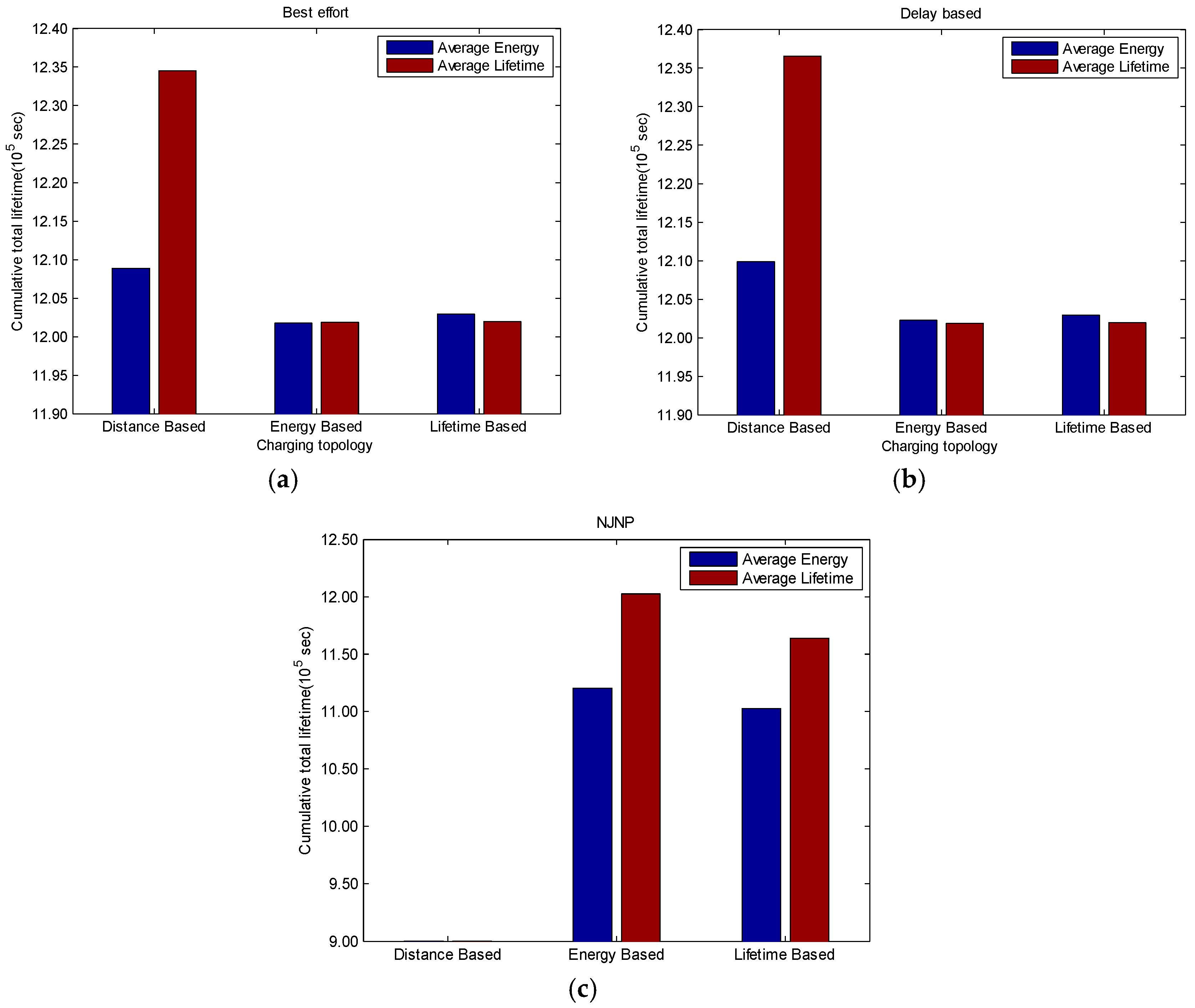
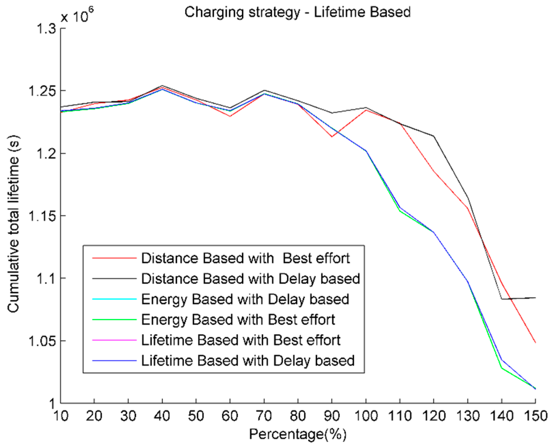
4.1. The Combination Experiment of Multi-Module Charging Strategy

Figure 9 shows the combination experiment of MMCS with different charging scheduling module. The x-axis and y-axis presents the charging topology and WRSNs’ total survival time, respectively, with two different charging strategies (based on the average energy module and average lifetime module). Figure 9a–c presents the MMCS with the best-effort charging module, MMCS with delay-based charging module, and MMCS with NJNP. Overall, MMCS with the best-effort and delay-based charging modules perform better than the NJNP in prolonging the WRSNs’ lifetime. However, all the combinations of MMCS provide different results because of the use of different charging topologies, charging schedules, and charging strategies. Further, Figure 9a,b shows that the distance-based topology is better than the energy-based and lifetime-based topologies. However, energy-based and lifetime-based topologies perform well in NJNP. This is because the NJNP considers only the next sensor node; considering the quantity of energy will enable it to rescue the most critical node.

However, to fulfill the goal of maximizing the survival time of the WRSNs, it should consider not only the energy but also the distance to prevent increasing the cost of WCV and delay. Therefore, the best combination of MMCS is the distance-based topology, delay-based charging schedule, and average lifetime charging strategy. The best combination is capable of prolonging the lifetime efficiently because it gives priority to the critical node and distance, and delay-based charging schedule considers the effect on the follow-up nodes.

4.2. Result of Return on Investment Analysis of Battery

Because the energy is exhausted, the group of batteries (B_c and B_m) need to be replaced. Therefore, additional cost is incurred for replacing the group of batteries (B_c and B_m). As shown in Equation (14), the return on investment (ROI) represents the extension in the lifetime achieved using a group of batteries. The results shown in Figure 10 are classified according to the charging strategies. Figure 10a presents the average energy charging strategy, whereas Figure 10b presents the average lifetime charging strategy. The x-axis and y-axis presents the charging topology and the extension in lifetime achieved by using the group of batteries, respectively. Overall, the average lifetime charging strategy provides higher ROI and gives credit to the different ED between nodes.

The average lifetime strategy calculates the ED according to the different energy consumptions between nodes, with the result that energy is replenished according to different energy consumptions. It ensures that the lifetime of nodes with different energy consumptions is the same. Although the best ROI is provided by the average lifetime charging strategy combined with lifetime-based topology, it was not the most efficient in terms of the total survival time of WRSNs.

$$ROI=\frac{\text{time of extended}}{\text{number of replacing the battery}}$$

(14)

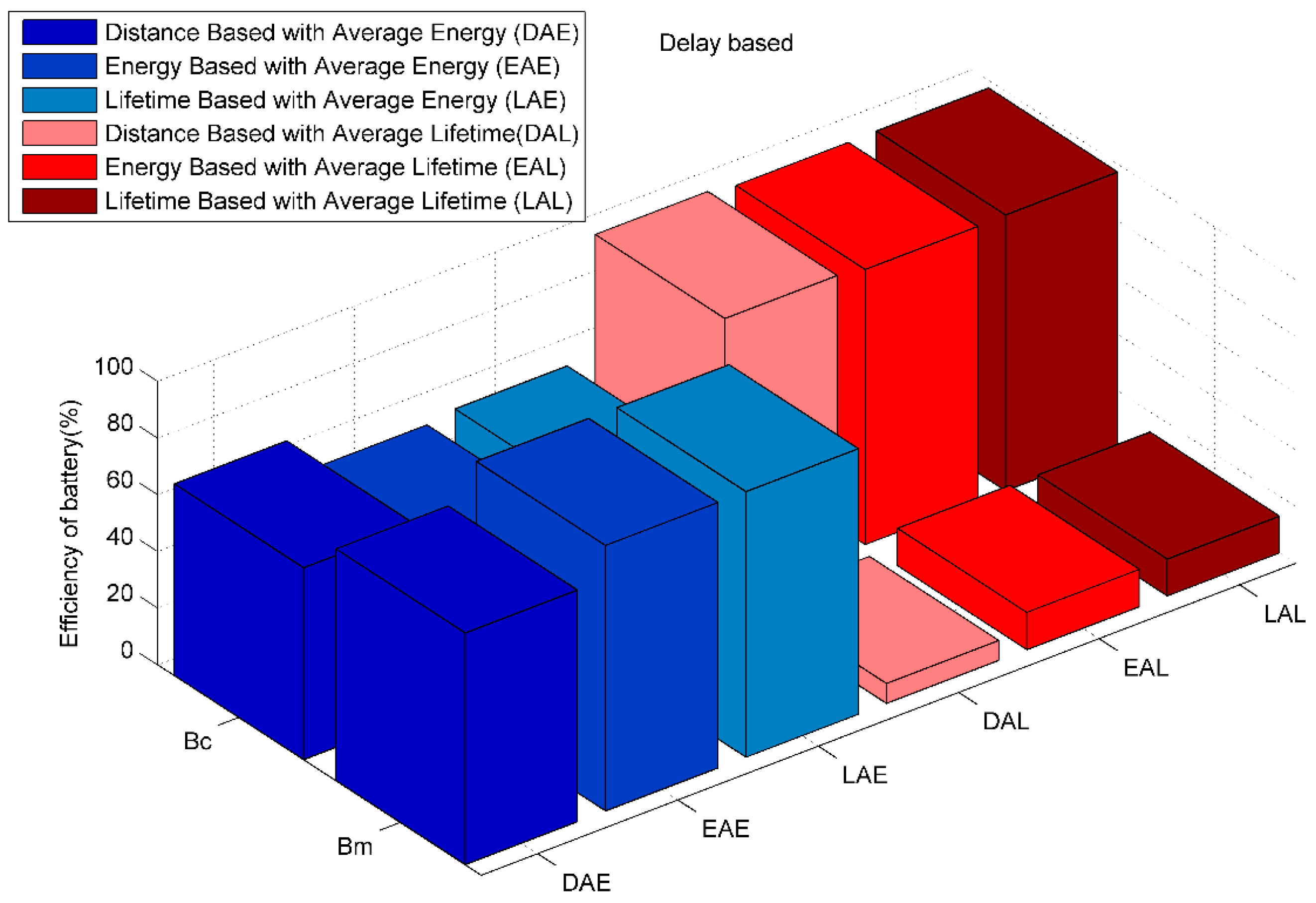
4.3. Efficiency of Battery

We observe that the average lifetime charging strategy is a better choice than the average energy strategy. In addition to the ROI, this paper further compares the usage efficiency. This section analyzed the effect of the charging strategy on B_m and B_c. In Figure 11, the x-axis presents the combination of charging topology and charging strategy, the y-axis presents the type of battery, and the z-axis presents the usage efficiency of the battery. The usage efficiency of the battery is calculated by Equation (15). Indeed, the most efficient battery is B_c, which is used in the average lifetime charging strategy. However, there is a great disparity between B_m and B_c in the average lifetime charging strategy. In contrast, it is more balanced between B_m and B_c in the average energy charging strategy. The unbalanced usage efficiency is caused by the oversized battery. It implies that a lot of energy is wasted at B_m and B_c while replacing the group of batteries. This analysis of the results is used to determine the capacity of the battery.

$$efficiency=\frac{\text{total power consumption}}{\text{number of battery used}}\times 100\%$$

(15)

4.4. Extended Lifetime of Wireless Rechargeable Sensor Networks

Figure 12 presents the extended lifetime of each sensor node obtained by the best combination of MMCS. The x-axis presents each sensor node, and the y-axis presents the total survival time of each sensor node. The red line depicts the situation without charging, and the blue line depicts the situation with the best combination of MMCS. The best combination of MMCS extends the lifetime of the nodes that were dead earlier, and it takes approximately 4166 s to extend the lifetime of WRSNs. This means that the MMCS added 2 days, 21 h, and 26 min to the WRSNs’ survival time.

4.5. Distribution of the Rescued Sensor Nodes

This section discusses the distribution of the rescued sensor nodes. In Figure 13, the sensor nodes are sorted according to the energy consumption rate in descending order, and grouped according to the number of E(N). This study discusses the rescue conditions of the top five groups. The x-axis presents the groups according to the number of E(N), and the y-axis presents the total extended lifetime of each sensor node.

The best combination of MMCS does the best job in rescuing the sensor nodes with a higher energy consumption rate, and the lifetime of the nodes with lower energy consumption rate is extended by a smaller amount. The energy of the dying sensor nodes are enhanced for prolonging the lifetime of the entire WRSN.

4.6. Comprehensive Comparison

This section presents a comprehensive comparison of the top three combinations of MMCS as shown in Figure 14. DDE denotes the combination of distance-based topology, delay-based charging schedule, and average energy charging strategy. DBL denotes the combination of distance-based topology, best effort-charging schedule, and average lifetime charging strategy. DDL denotes the combination of distance-based topology, delay-based charging schedule, and average lifetime charging strategy. The score of each aspect is calculated by Equation (16). DBL and DDL provide better performance. Furthermore, compared to DBL, DDL scores higher on every aspect, except on B_m’s efficiency.

$${score}_{\text{aspect}}=\frac{\text{original score of the aspect}-\text{the lowest score in the aspect}}{\text{the highest score in the aspect}-\text{the lowest score in the aspect}}\times 100\%$$

(16)

4.7. Effect of Variation of the Amount of Charge

It is known that the average lifetime-charging strategy performs better in extending the lifetime. This paper further discusses the effect of the amount of charge. The experiment only varies the charging quantity in the best combination of MMCS, and the changing interval varies from 10% to 150% of ED. The result is shown in Figure 15, in which the x-axis presents the percentage of ED and the y-axis presents the total survival time of WRSNs. It is found that a larger charging quantity cannot increase the lifetime. Similarly, a lower charging quantity also cannot increase the lifetime by any significant amount.

A larger charge quantity requires more time to charge the sensor node, which may lead to the node’s death in the charging process. However, lower charging quantity is not effective in prolonging the lifetime. Therefore, it is very important to balance the charging time and charging quantity. From the results, the charging quantity is reduced to 40%–70% ED calculated by the average lifetime charging strategy, which provides the best performance in terms of prolonging the lifetime.

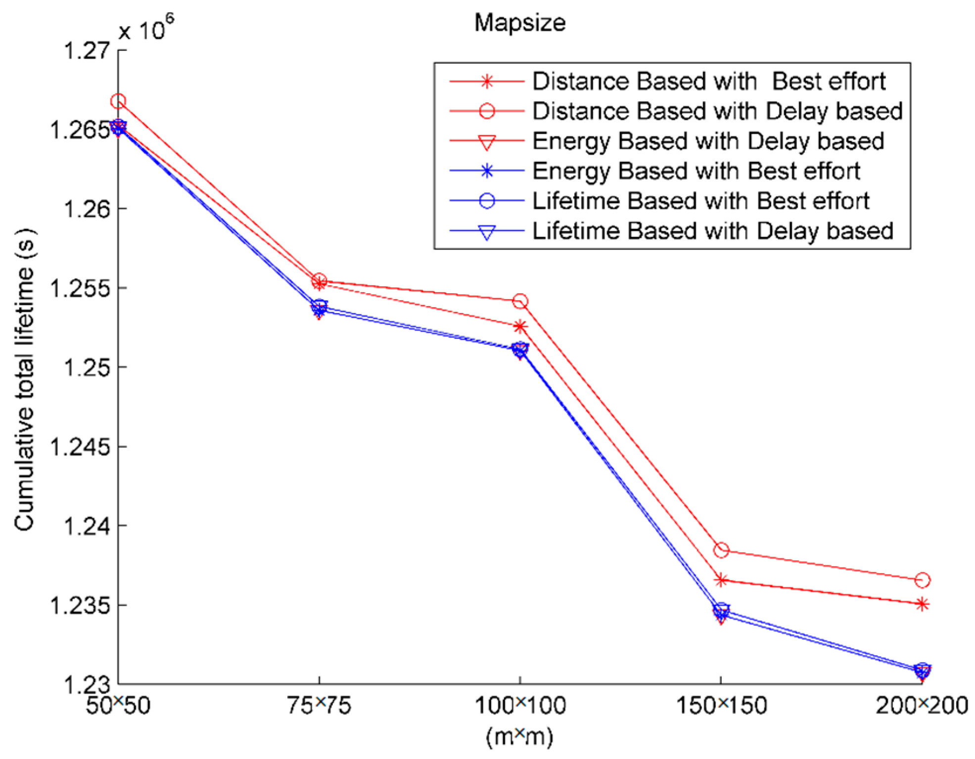
4.8. The Analysis of Density

In addition to the effect of charging quantity on the results, this paper also explores the effect of the distribution of the sensor nodes on the charging efficacy. This paper tests five different map sizes from 50 m × 50 m to 200 m × 200 m, and implements them with the average lifetime charging strategy. From the results shown in Figure 16, it is seen that MMCS performs better in high-density areas. This is because the map size affects the density of sensor nodes, and the WCV requires more time for moving. In an empty environment, the sensor nodes may die during the movement of the WCV. On the contrary, WCV’s better performance in rescuing the sensor nodes is attributable to the decrease in the time spent on moving.

5. Conclusions

The optimized charging path problem is the most widely discussed issue in employing WRSNs with WCV. This problem involves determining the most efficient path for charging sensor nodes. Further, charging-scheduling problems also need to be considered in the optimized charging path problem. In this paper, we proposed a MMCS used to prolong the lifetime of the entire WRSN. MMCS can be divided into three stages: the charging topology, charging scheduling, and charging strategy stages, with multiple modules in each stage. The best module combination of MMCS is the distance-based module in the charging topology stage, delay-based module in the charging schedule stage, and the average lifetime module in the charging strategy stage. The best module combination enables prolonging the lifetime efficiently, as it considers not only the priority of urgent nodes but also the travel distance of WCV; the delay-based module of the charging schedule stage considers the delay effect on the follow-up nodes. The experimental results show that the proposed MMCS can improve the lifetime of the entire WRSN and that it significantly outperforms the NJNP method in terms of lifetime improvement of the entire WRSN. In the future, we will consider more than one WCV and multi-point charging technology in the optimized charging path problem.

References

1. Shi, Y.; Xie, L.; Thomas Hou, Y.; Sherali, H.D. On renewable sensor networks with wireless energy transfer. In Proceedings of the 2011 IEEE International Conference on Computer Communications (INFOCOM), Shanghai, China, 10–15 April 2011; pp. 1350–1358.
2. Xie, L.; Shi, Y.; Thomas Hou, Y.; Sherali, H.D. Making sensor networks immortal: An energy-renewal approach with wireless power transfer. IEEE/ACM Trans. Netw. 2012, 20, 1748–1761. [Google Scholar] [CrossRef]
3. Kurs, A.; Karalis, A.; Moffatt, R.; Joannopoulos, J.D.; Fisher, P.; Soljačić, M. Wireless power transfer via strongly coupled magnetic resonances. Science 2007, 317, 83–86. [Google Scholar] [CrossRef] [PubMed]
4. Xie, L.; Shi, Y.; Thomas Hou, Y.; Lou, W.; Sherali, H.D.; Midkiff, S.F. On renewable sensor networks with wireless energy transfer: The multi-node case. In Proceedings of the 2012 9th Annual IEEE Communications Society Conference on Sensor, Mesh and Ad Hoc Communications and Networks (SECON), Seoul, Korea, 18–21 June 2012; pp. 10–18.
5. Xie, L.; Shi, Y.; Thomas Hou, Y.; Lou, A. Wireless power transfer and applications to sensor networks. IEEE Wirel. Commun. 2013, 20, 140–145. [Google Scholar]
6. Xie, L.; Shi, Y.; Thomas Hou, Y.; Lou, W.; Sherali, H.D.; Midkiff, S.F. Bundling mobile base station and wireless energy transfer: Modeling and optimization. In Proceedings of the 2013 Proceedings IEEE International Conference on Computer Communications (INFOCOM), Turin, Italy, 14–19 April 2013; pp. 1636–1644.
7. Xie, L.; Shi, Y.; Thomas Hou, Y.; Lou, W.; Sherali, H.D.; Zhou, H.; Midkiff, S.F. A mobile platform for wireless charging and data collection in sensor networks. IEEE J. Sel. Areas Commun. 2015, 33, 1521–1533. [Google Scholar] [CrossRef]
8. Guo, S.; Wang, C.; Yang, Y. Mobile data gathering with wireless energy replenishment in rechargeable sensor networks. In Proceedings of the 2013 Proceedings IEEE International Conference on Computer Communications (INFOCOM), Turin, Italy, 14–19 April 2013; pp. 1932–1940.
9. Fu, L.; Cheng, P.; Gu, Y.; Chen, J.; He, T. Minimizing charging delay in wireless rechargeable sensor networks. In Proceedings of the 2013 Proceedings IEEE International Conference on Computer Communications (INFOCOM), Turin, Italy, 14–19 April 2013; pp. 2922–2930.
10. Hu, C.; Wang, Y.; Zhou, L. Make Imbalance Useful. In Joint International Conference on Pervasive Computing and the Networked World; Springer International Publishing: Istanbul, Turkey, 2013; pp. 160–171. [Google Scholar]
11. Gross, D.; Shortle, J.F.; Thompson, J.M.; Harris, C.M. Fundamentals of Queueing Theory, 4th ed.; John Wiley & Sons: New York, NY, USA, 2008. [Google Scholar]
12. Peng, Y.; Li, Z.; Zhang, W.; Qiao, D. Prolonging sensor network lifetime through wireless charging. In Proceedings of the 2010 IEEE 31st Real-Time Systems Symposium (RTSS), San Diego, CA, USA, 30 November–3 December 2010; pp. 129–139.
13. He, L.; Gu, Y.; Pan, J.; Zhu, T. On-demand charging in wireless sensor networks: Theories and applications. In Proceedings of the 2013 IEEE 10th International Conference on Mobile Ad-Hoc and Sensor Systems, Hangzhou, China, 14–16 October 2013; pp. 28–36.
14. He, L.; Gu, Y.; Pan, J.; Zhu, T. Evaluating the on-demand mobile charging in wireless sensor networks. IEEE Trans. Mob. Comput. 2015, 14, 1861–1875. [Google Scholar] [CrossRef]
Figure 1. A wireless sensor networks with a wireless charging vehicle (WCV).
Energies 09 00664 g001
Figure 2. Wireless sensor network with a WCV using cell centers to find stay points on the traveling path.
Energies 09 00664 g002
Figure 3. Example of WRSNs.
Energies 09 00664 g003
Figure 4. The schematic diagram of MMCS.
Energies 09 00664 g004
Figure 5. Best-effort module algorithm.
Energies 09 00664 g005
Figure 6. Delay-based module algorithm.
Energies 09 00664 g006
Figure 7. The schematic diagram of delay caused by charging order.
Energies 09 00664 g007
Figure 8. The topology of the example.
Energies 09 00664 g008
Figure 9. The combination experiment of MMCS with different charging scheduling module (a) MMCS with the best effort-charging module; (b) MMCS with delay-based charging module; and (c) MMCS with NJNP.
Energies 09 00664 g009
Figure 10. Result of return on investment (ROI) analysis of battery.
Energies 09 00664 g010
Figure 11. Efficiency of battery.
Energies 09 00664 g011
Figure 12. Extended lifetime of WRSNs.
Energies 09 00664 g012
Figure 13. Distribution of the rescued sensor nodes.
Energies 09 00664 g013
Figure 14. Comprehensive comparison.
Energies 09 00664 g014
Figure 15. Result of charging quantity effect.
Energies 09 00664 g015
Figure 16. The analysis results of different density effect.
Energies 09 00664 g016