Diffusion Length Mapping for Dye-Sensitized Solar Cells

Abstract

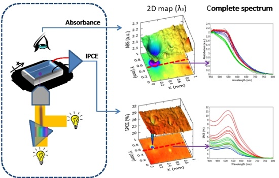
The diffusion length (L) of photogenerated carriers in the nanoporous electrode is a key parameter that summarizes the collection efficiency behavior in dye-sensitized solar cells (DSCs). At present, there are few techniques able to spatially resolve L over the active area of the device. Most of them require contact patterning and, hence, are intrinsically destructive. Here, we present the first electron diffusion length mapping system for DSCs based on steady state incident photon to collected electron (IPCE) conversion efficiency (${\mathsf{\eta }}_{IPCE}$) analysis. The measurement is conducted by acquiring complete transmittance ($T_{\text{DSC}}$) and ${\mathsf{\eta }}_{IPCE}$ spectra from the photo electrode (PE) and counter electrode (CE) for each spatial point in a raster scan manner. $L(x,y)$ is obtained by a least square fitting of the IPCE ratio spectrum ($IPC{E}_{\text{R}}=\frac{{\mathsf{\eta }}_{IPCE\text{-CE}}}{{\mathsf{\eta }}_{IPCE\text{-PE}}}$). An advanced feature is the ability to acquire ${\mathsf{\eta }}_{IPCE}$ spectra using low-intensity probe illumination under weakly-absorbed background light (625 nm) with the device biased close to open circuit voltage. These homogeneous conditions permit the linearization of the free electron continuity equation and, hence, to obtain the collection efficiency expressions (${\mathsf{\eta }}_{\text{COL-PE}}$ and ${\mathsf{\eta }}_{\text{COL-CE}}$). The influence of the parameter’s uncertainty has been quantified by a sensitivity study of L. The result has been validated by quantitatively comparing the average value of L map with the value estimated from electrochemical impedance spectroscopy (EIS).

1. Introduction

It has long been recognized that the spatial distribution of local parameters, such as optical absorption, electroluminescence, diffusion length, etc., can provide valuable information on the stability, performance and degradation prediction of solar cells [1,2]. Moreover, spatial visualization of these properties is crucial to better address the up-scaling procedure that every photovoltaic technology has to tackle [3]. Mapping techniques can be grouped into ex situ and in situ methods according, respectively, to the need for cell disassembly or not [4]. We will focus our attention on in situ mapping techniques that are based on optical probes, such as Raman [5,6], transmittance-reflectance and photo-luminescence [7] microscopy and electro-optical techniques [8], such as light-beam-induced current (LBIC) [9,10,11] and electro-luminescence [12] microscopy. The good performances of DSCs require improving the charge collection efficiency over the entire semiconducting electrode (generally, titanium dioxide (TiO${}_2$)) to the contact [13,14]; in particular, the electronic property and the surface area of the photoanode determine the current output of the device [13,15]. Accordingly, good light harvesting ability, charge transport and low recombination are key challenges for hybrid solar cells [16,17]. The charge collection capability of the photoanode is quantified with the diffusion length of the injected charges; recent papers present an LBIC-based technique [18,19,20] to directly extract the absolute value of L; unfortunately, despite the simplicity of the analysis, these techniques require a substrate contact patterning that limits the application to customized devices. Here, we present a new in situ technique, spectrally-resolved analysis by transmittance and efficiency mapping (SATEM), to extract the (L) distribution by contemporary mapping the transmittance ($T_{\text{DSC}}$) and the incident photons to current conversion efficiency (${\mathsf{\eta }}_{IPCE}$). As such, SATEM provides 2D maps of both electro-optical and topographic information simultaneously. The L estimation is based on an accurate modeling of the incident photon to collected electron (IPCE) spectra, as already discussed by Barnes et al. [21,22] and Jennings et al. [23]. Therefore, spectrally-resolved mapping of the IPCE ratio ($IPC{E}_{\text{R}}$) and $T_{\text{DSC}}$ contains more information on physical and electrochemical solar cell properties than classical LBIC techniques. We introduced SATEM analysis in a recent article [24] focused on the degradation mechanisms induced by the reverse bias condition on the large area DSC module (five cells of 3.6 cm${}^2$ each); spatially-resolved transmittance and IPCE spectra were combined with the resonance Raman technique to investigate the effect of by-products on the regeneration efficiency of the dye and the free charge recombination losses inside the TiO${}_2$ film. Moreover, the ability to tune both the background and monochromatic beam was used to highlight areas with trap-limited charge collection and the limitation of iodide diffusion. Differently, in the present work, we demonstrate that the combination of an SATEM analysis with an accurate modeling can provide the spatial distribution of L. In order to confirm the results, electrochemical impedance spectroscopy (EIS) has been chosen as the independent determination of L; in particular, the average value of L provided by SATEM analysis (the steady state technique) is in agreement with the value extracted from the fitting of the EIS spectra (the dynamic technique).

2. Theoretical Basis

The diffusion length, considered normal to the plane of the film, is the average distance an injected electron can travel through the cell before recombining with tri-iodide ions or oxidized dye species. If L is lower than the TiO${}_2$ film thickness ($L<d$), only a small injected charge fraction will be collected, making a long diffusion length desirable [25]. Assuming a first order recombination in free electron concentration, the electron diffusion length can be defined as $L=\sqrt{D_{\text{n}}{\mathsf{\tau }}_{\text{n}}}$, where $D_{\text{n}}$ is the diffusion coefficient of electrons in the conduction band of the TiO${}_2$ and ${\mathsf{\tau }}_{\text{n}}$ is the free electron lifetime.

2.1. Estimation of L from Electrochemical Impedance Spectroscopy Measurements

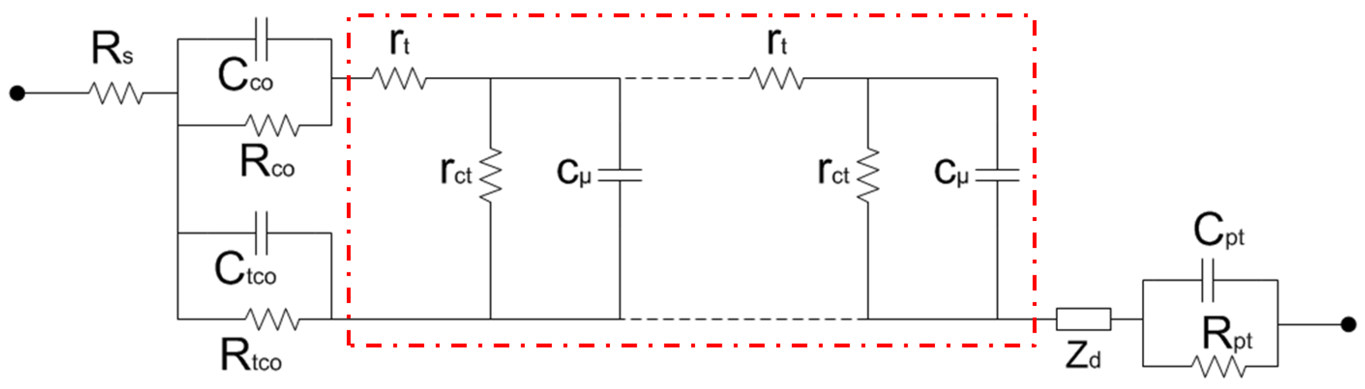
Following the suggestion of Jennings et al. [23], EIS analysis has been chosen to quantitatively validate the SATEM results. In particular, EIS experiments can be performed under the same homogeneous conditions of SATEM (open circuit voltage bias condition with weekly-absorbed background light), unlike other dynamic techniques (transient photocurrent and intensity-modulated photocurrent spectroscopy [26]) that operate under short circuit conditions. The diffusion length of DSCs is well defined from the impedance Z of the cell estimated by EIS [14,27,28,29]. The EIS technique is based on the superimposing of a small amplitude harmonic AC voltage modulation on the DC voltage of the cell for a set of frequencies and by measuring the resulting AC current. The final impedance spectrum can be fitted with a suitable electrical circuit model generally based on a transmission line that models the TiO${}_2$ layer [30]. The model used in our analysis (Figure 1) is discussed in detail in several works [30,31,32]. The distributed resistance $r_{\text{t}}$ (total resistance $R_{\text{t}}=r_{\text{t}}d$) represents the local resistance to electron transport in the TiO${}_2$ layer that is related to the carrier concentration ($n_{\text{c}}$) and diffusion coefficient ($D_{\text{n}}$). The distributed component $r_{\text{ct}}$ (total resistance $R_{\text{ct}}=\frac{r_{\text{ct}}}{d}$) models the local resistance to the charge transfer across the TiO${}_2$-electrolyte layer that is determined by $n_{\text{c}}$ and the free electron lifetime (${\mathsf{\tau }}_{\text{n}}$). The diffusion length is then defined as:

$$L=d\sqrt{\frac{R_{\text{ct}}}{R_{\text{t}}}}$$

(1)

Since the measured $R_{\text{ct}}$ and $R_{\text{t}}$ are an averaged value of the local contributions over the TiO${}_2$ thickness, the homogeneous conditions are indispensable to obtain a reliable estimation of the collection capability of the photoelectrode and, hence, of the absolute value of L. In particular, EIS analysis under illumination at open circuit allows characterizing $r_{\text{t}}$ and $r_{\text{ct}}$ under the flat quasi-Fermi level unlike what happens under dark and forward bias [17,26,33]. The disadvantage of the impedance method is that it becomes difficult to measure the transport phenomena at high light intensities, particularly in the case of cells with long diffusion lengths, where $r_{\text{t}}$ becomes much smaller than the series and cathode impedance at open circuit voltages and fitting becomes unreliable.

2.2. Estimation of L from Incident Photon to Collected Electron Measurements

The ${\mathsf{\eta }}_{IPCE}$ is composed of three components, such that:

$${\mathsf{\eta }}_{\text{IPCE}}\left(\mathsf{\lambda }\right)=\frac{j_{\text{SC}}\left(\mathsf{\lambda }\right)}{q\mathsf{\varphi }\left(\mathsf{\lambda }\right)}={\mathsf{\eta }}_{\text{LH}}\left(\mathsf{\lambda }\right){\mathsf{\eta }}_{\text{sep}}\left(\mathsf{\lambda }\right){\mathsf{\eta }}_{\text{col}}\left(\mathsf{\lambda }\right)$$

(2)

where $j_{\text{SC}}$ is the short-circuit current, q is the elementary charge, $\mathsf{\varphi }$ is the photon flux density, ${\mathsf{\eta }}_{\text{LH}}$ is the efficiency of photon harvesting by dye molecules, ${\mathsf{\eta }}_{\text{sep}}$ is the charge separation efficiency and ${\mathsf{\eta }}_{\text{col}}$ is the electron collection from the TiO${}_2$ to the external circuit [14].

In semitransparent DSCs, the ones discussed in this work, ${\mathsf{\eta }}_{IPCE}$ can be measured from the photo electrode (PE) or counter electrode (CE) side. In the following, we differentiate the parameters obtained with PE or CE side illumination by the PE or CE subscript, respectively. As proposed by Halme et al. [34], a simple analytic expressions of ${\mathsf{\eta }}_{\text{LH},\text{PE}}$ and ${\mathsf{\eta }}_{\text{LH},\text{CE}}$ can be derived from the optical model shown in Figure 2.

$${\mathsf{\eta }}_{\text{LH},\text{PE}}=T_{\text{TCO}}\left(1-R_{\text{PE}}\right)\frac{{\mathsf{\alpha }}_{\mathrm{D}}}{\mathsf{\alpha }}\left(1-e^{-\mathsf{\alpha }d}\right)$$

(3)

$${\mathsf{\eta }}_{\text{LH},\text{CE}}=T_{\text{CE}}{T}_{\text{EL}}\left(1-R_{\text{PE}}\right)\frac{{\mathsf{\alpha }}_{\mathrm{D}}}{\mathsf{\alpha }}\left(1-e^{-\mathsf{\alpha }d}\right)$$

(4)

where $T_{\text{TCO}}$, $T_{\text{CE}}$ and $T_{\text{EL}}$ are the transmittances of the TCO-coated glass substrate of the photoelectrode, the counter electrode and the free-electrolyte, respectively. $R_{\text{PE}}$ is the photoelectrode film reflectance, and d is its thickness. $\mathsf{\alpha }$ is the absorption coefficient of the electrolyte-filled dyed photoelectrode film:

$$\mathsf{\alpha }\left(\mathsf{\lambda }\right)={\mathsf{\alpha }}_{\text{D}}\left(\mathsf{\lambda }\right)+\mathsf{ϵ}\left(\mathsf{\lambda }\right)P{\mathsf{\alpha }}_{\text{EL}}\left(\mathsf{\lambda }\right)$$

(5)

where ${\mathsf{\alpha }}_{\text{D}}$ is the absorption coefficient of the dyed photoelectrode film, ${\mathsf{\alpha }}_{\text{EL}}$ is the absorption coefficient of the bulk electrolyte solution, P is the porosity of the film (assumed to be 0.5) and $\mathsf{ϵ}$ is the average optical mean path length parameter that takes into account light scattering phenomena (a value of 1.5 is assumed here). Analytic expressions of the collection efficiencies are obtained by the resolution of the steady state free-electron continuity equation:

$$\frac{\partial n_{\text{c}}}{\partial t}={\mathsf{\eta }}_{\text{reg}}\left(n_{\text{c}}\left(x\right)\right)G\left(x\right)+D_{\text{n}}\frac{{\partial }^2{n}_{\text{c}}\left(x\right)}{\partial x^2}-k_{\text{n}}^{\prime }{\left(n_{\text{c}}\left(x\right)-n_{\text{eqm}}\right)}^{{\mathsf{\gamma }}_{\text{n}}}=0$$

(6)

where ${\mathsf{\eta }}_{\text{reg}}$ is the sensitizer regeneration efficiency expressed as:

$${\mathsf{\eta }}_{\text{reg}}\left(n_{\text{c}}\left(x\right)\right)=\frac{k_{\text{r}}^{\prime }}{k_{\text{g}}{\left(n_{\text{c}}\left(x\right)-n_{\text{eqm}}\right)}^{{\mathsf{\gamma }}_{\text{g}}}+k_{\text{r}}^{\prime }}$$

where $n_{\text{c}}$ is the equilibrium concentration of free electrons in the dark, $G\left(x\right)$ is the position-dependent photogeneration rate, $D_{\text{n}}$ is the diffusion coefficient of free electrons, $k_{\text{n}}^{\prime }$ and $k_{\text{g}}$ are rate constants for recombination of electrons with tri-iodide and oxidized sensitizer molecules, respectively, $k_{\text{r}}^{\prime }$ is the rate constant for the sensitizer regeneration reaction with iodide, ${\mathsf{\gamma }}_{\text{n}}$ and ${\mathsf{\gamma }}_{\text{g}}$ are the reaction orders with respect to free electron concentration and $n_{\text{eqm}}$ is the free electron concentration at thermal equilibrium in the dark.

2.2.1. Linearization of the Free Electron Continuity Equation

Classical expressions of ${\mathsf{\eta }}_{\text{col},\text{PE-CE}}$ are obtained from a linearization of the free electron continuity equation, where a first order recombination with tri-iodide (${\mathsf{\gamma }}_{\text{n}}=1$) and a negligible recombination with oxidized dye ($k_{\text{g}}=0$) are assumed [25,32,35]. These assumptions are the main cause of the discrepancies between different methodological approaches that estimate the diffusion length parameter [22,23,34,36]. For a position-independent background generation rate, $G_{\text{bg}}$, and electron concentration (i.e., open-circuit condition), $n_{\text{bg}}$, the free electron continuity equation for $n_{\text{bg}}$ can be written as ${\text{I}}^{-}$:

$$\frac{\partial n_{\text{bg}}}{\partial t}={\mathsf{\eta }}_{\text{reg}}{G}_{\text{bg}}-k_{\text{n}}^{\prime }{n}_{\text{bg}}^{{\mathsf{\gamma }}_{\text{n}}}=0$$

Then, the background generation rate can be written as:

$$G_{\text{bg}}=\frac{k_{\text{n}}^{\prime }{n}_{\text{bg}}^{{\mathsf{\gamma }}_{\text{n}}}}{{\mathsf{\eta }}_{\text{reg}}}$$

(7)

Assuming small perturbations of $G\left(x\right)$ around $G_{\text{bg}}$ and $n_{\text{c}}\left(x\right)$ around $n_{\text{bg}}$, Equation (6) can be linearized resulting in a familiar equation with a linear recombination term:

$$\frac{\partial n_{\text{c}}\left(x\right)}{\partial t}\approx {\mathsf{\eta }}_{\text{reg}}\left(G\left(x\right)-G_{\text{bg}}\right)-D_{\text{n}}\frac{{\partial }^2{n}_{\text{c}}\left(x\right)}{\partial x^2}-\widehat{k_{\text{n}}}\left(n_{\text{c}}\left(x\right)-n_{\text{bg}}\right)$$

(8)

where:

$$\widehat{k_{\text{n}}}=k_{\text{n}}^{\prime }{n}_{\text{bg}}^{{\mathsf{\gamma }}_{\text{n}}-1}\left({\mathsf{\gamma }}_{\text{n}}+{\mathsf{\gamma }}_{\text{g}}\left(1-{\mathsf{\eta }}_{\text{reg}}\right)\right)$$

From Equation (8), it follows that existing solutions to the electron continuity equation remain valid, even for ${\mathsf{\gamma }}_{\text{n}}\ne 1$ and non-negligible recombination with oxidized sensitizer molecules. This conclusion applies to the employed characterization techniques; therefore, if the provided measurements are performed under homogeneous conditions, the expressions of electron collection efficiency ${\mathsf{\eta }}_{\text{col},\text{PE-CE}}$ can be described by the standard diffusion model of electron generation, transport and recombination at the nanostructured photoelectrode introduced originally for DSCs by Sodergen et al. [25]:

$${\mathsf{\eta }}_{\text{col},\text{PE}}=\frac{\left[-L\mathsf{\alpha }cosh\left(\frac{d}{L}\right)+sinh\left(\frac{d}{L}\right)+L\mathsf{\alpha }{e}^{-\mathsf{\alpha }d}\right]L\mathsf{\alpha }}{\left(1-e^{-\mathsf{\alpha }d}\right)\left(1-L^2{\mathsf{\alpha }}^2\right)cosh\left(\frac{d}{L}\right)}$$

(9)

$${\mathsf{\eta }}_{\text{col},\text{CE}}=\frac{\left[L\mathsf{\alpha }cosh\left(\frac{d}{L}\right)+sinh\left(\frac{d}{L}\right)-L\mathsf{\alpha }{e}^{-\mathsf{\alpha }d}\right]L\mathsf{\alpha }{e}^{-\mathsf{\alpha }d}}{\left(1-e^{-\mathsf{\alpha }d}\right)\left(1-L^2{\mathsf{\alpha }}^2\right)cosh\left(\frac{d}{L}\right)}$$

(10)

2.2.2. Incident Photon to Collected Electron Ratio

Considering that ${\mathsf{\eta }}_{\text{sep}}$ can be assumed independent upon the light direction (PE or CE side) [21,34], it follows from Equations (3), (4), (9) and (10) that the $IPC{E}_{\text{R}}$ is given by:

$$IPC{E}_{\text{R}}=\frac{T_{\text{CE}}{T}_{\text{EL}}}{T_{\text{TCO}}}·\frac{\left[cosh\left(\frac{d}{L}\right)+\frac{1}{L\mathsf{\alpha }}sinh\left(\frac{d}{L}\right)\right]·e^{-\mathsf{\alpha }d}-1}{-cosh\left(\frac{d}{L}\right)+\frac{1}{L\mathsf{\alpha }}sinh\left(\frac{d}{L}\right)+e^{-\mathsf{\alpha }d}}$$

(11)

The expression can be improved by introducing the analytic expression $T_{\text{DSC}}$, that is experimentally obtained from SATEM:

$$T_{\text{DSC}}=T_{\text{TCO}}{T}_{\text{EL}}{T}_{\text{CE}}{T}_{\text{film}}=T_{\text{TCO}\mid \text{EL}\mid \text{CE}}\left(1-R_{\text{PE}}\right)e^{-\mathsf{\alpha }d}$$

(12)

where $T_{\text{TCO}\mid \text{EL}\mid \text{CE}}=T_{\text{TCO}}{T}_{\text{EL}}{T}_{\text{CE}}$ represents the transmittance of a cell composed of the CE and electrolyte, and its spectrum is extracted and averaged over the perimeter points around the active area of the cell. $IPC{E}_{\text{R}}$ can be rearranged as follow:

$$IPC{E}_{\text{R}}=\frac{T_{\text{DSC}}}{T_{\text{TCO}}^2·\left(1-R_{\text{PE}}\right)e^{-\mathsf{\alpha }d}}·\frac{\left[cosh\left(\frac{d}{L}\right)+\frac{1}{L\mathsf{\alpha }}sinh\left(\frac{d}{L}\right)\right]·e^{-\mathsf{\alpha }d}-1}{-cosh\left(\frac{d}{L}\right)+\frac{1}{L\mathsf{\alpha }}sinh\left(\frac{d}{L}\right)+e^{-\mathsf{\alpha }d}}$$

(13)

The spatially-resolved absorbance coefficient ($\mathsf{\alpha }$) is obtained by inverting Equation (12):

$$\mathsf{\alpha }=\frac{ln\left(\frac{\left(1-R_{\text{PE}}\right)T_{\text{TCO}\mid \text{EL}\mid \text{CE}}}{T_{\text{DSC}}}\right)}{d}$$

(14)

On the contrary, $T_{\text{TCO}}$, $R_{\text{PE}}$ and d are provided by independent measurements, but it is important to reiterate that: the spatial variation $T_{\text{TCO}}$ can be assumed negligible; the spatial variation of d is averaged by increasing the spot size of the optical probe during the spectral resolved mapping; and as will be shown in the sensitivity analysis, the influence of $R_{\text{PE}}$ over the estimation of L is demonstrated to be irrelevant. Equation (13) can be fitted to experimental $IPC{E}_{\text{R}}$ with L and d as the only free-fitting parameters. By allowing also d to vary around the experimental value, a better fitting to the spectra is obtained without the influence of the value of L [23].

3. Scanning Apparatus (Spectrally-Resolved Analysis by Transmittance and Efficiency Mapping)

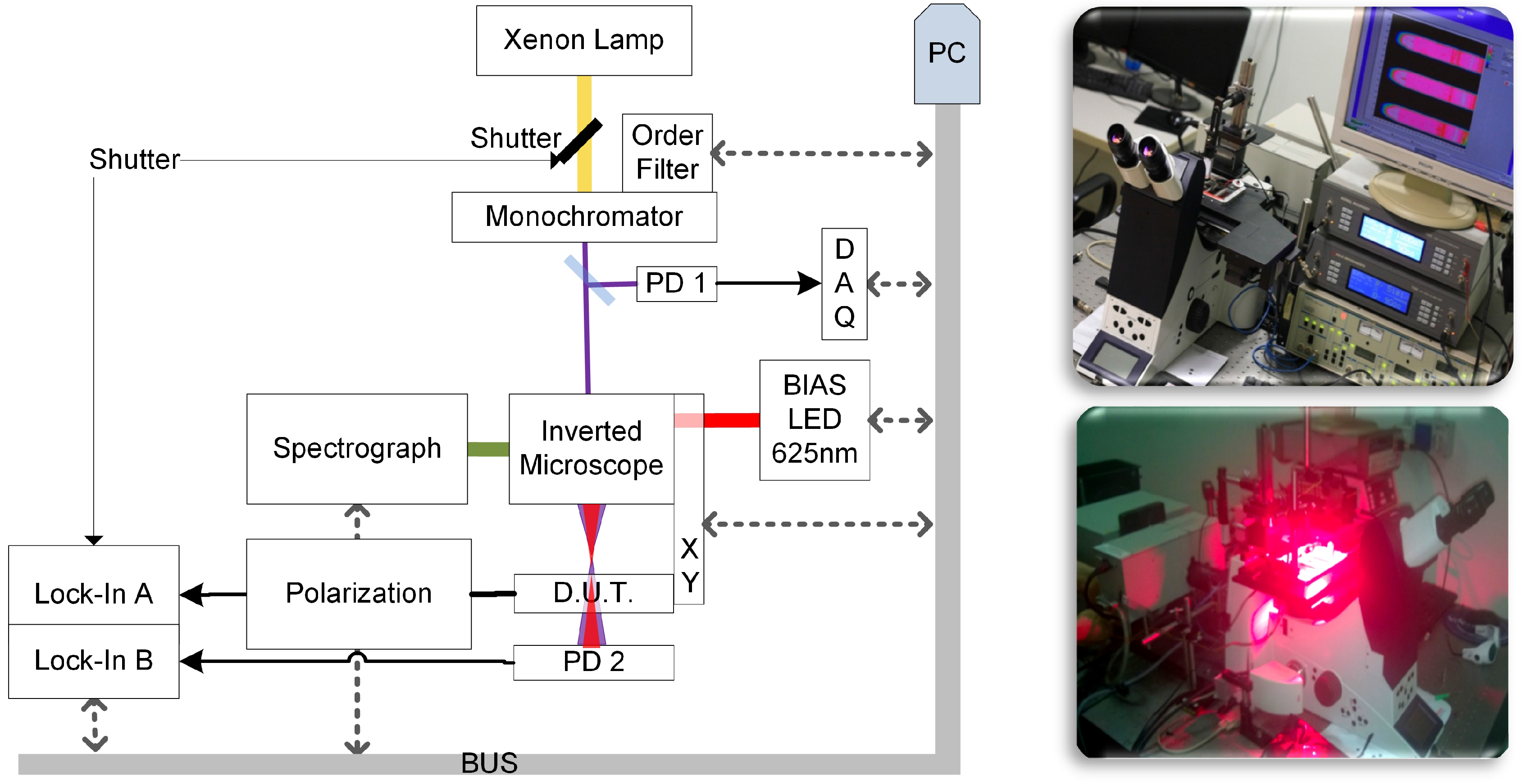
The SATEM system (Figure 3) is built around an inverted microscope DMI 5000 from Leica (Wetzlar, Germany) that includes a charge-coupled device (CCD) camera, a motorized XY stage and two optical entrances; one of the latter is dedicated to the monochromatic light coming from a Xenon lamp (200 W Apex Source Model 66450) and a monochromator ($\frac{1}{8}$ m Cornerstone 130) from Newport, Irvine, CA, USA. The spectral resolution is 2 nm on a range from 300 nm to 1000 nm. The sample is completely illuminated from the back-side with a red light-emitting diode array (Oslon ILR-ON 625 nm 20 W from Osram, Munich, Germany) that allows one to fix an irradiation level up to the 1.5 sun in the visible range of 2 cm${}^2$. The absorption length calculated at 625 nm over the TiO${}_2$ film is ca. 10 $\mathsf{\mu }$m, approximately equal to the commonly-used layer thicknesses. The background light of the red led array is fine-tuned in order to ensure the same V${}_{\text{oc}}$ for PE and CE illuminations. The transmitted optical signal can be registered either by a large area photodetector ($P{D}_2$, Model FDS 1010 from Thorlabs, Newton, NJ, USA) close to the back side of the device or an integrating sphere, depending on the device layout and scattering phenomena. The short circuit currents of the device and $P{D}_2$ are discriminated in a phase-sensitive detection system composed of an optical chopper (Newport Model 75159) and two digital lock-in amplifiers (Eg&g 7265 from Signal Recovery, Oak Ridge, TN, USA). Frequency modulation in the sub-Hz range is necessary to avoid the underestimation of the IPCE value [37]. An embedded transimpedance amplifier connected to $P{D}_1$ and a data acquisition board (Model 9205 from National Instruments, Austin, TX, USA) provides the incident optical power information. Thanks to the simultaneous acquisitions of the incident ($P{D}_1$) and transmitted ($P{D}_2$) optical powers and short circuit current of the device, spectra and maps of both IPCE and transmittance will be independent of possible fluctuations of the monochromatic light source. The system is completely automated under the LabVIEW programming environment, and the IPCE/transmittance spectra are acquired and elaborated in parallel.

The advantages of the SATEM approach over previous spectroscopic and scanned probe studies are: (i) direct spatial correlation between optical (transmittance) and electro-optical (${\mathsf{\eta }}_{IPCE}$) information; (ii) the ability to extract wide spectra (350–1100 nm) with 2 nm of resolution; (iii) differential IPCE with localized white bias light (tunable up to 1.5 sun) to investigate electron collection and mass transport limitations [38,39,40]; (iv) sub-Hz optical chopping frequency to avoid the underestimation of the IPCE spectrum [41,42,43,44]; and (v) lamp power fluctuation immunity thanks to simultaneous acquisition of incident and transmitted optical signals and the short circuit current of the sample.

4. Results and Discussion

In order to focus attention on the potential of the technique rather than the specific device under study, a standard and stable DSC configuration has been chosen; in particular, a commercial iodine-based electrolyte (HSE) and Z907 sensitizer [45] from Dyesol (Queanbeyan, Australia) ensured an excellent stability that helped during extended measurements.

4.1. Sensitivity Analysis

Since the spatial estimation of L requires a nontrivial fitting procedure with several parameters involved, we conducted a sensitivity study in order to quantify the influence of parameter uncertainty ($e_{x_i}$) on the L. In particular, $x_i$ stands for d, $\mathsf{\alpha }$, $R_{\text{PE}}$, $T_{\text{DSC}}$, $T_{\text{TCO}}$, ${\mathsf{\eta }}_{IPCE,\text{PE}}$ and ${\mathsf{\eta }}_{IPCE,\text{CE}}$. The SATEM system acquires $T_{\text{DSC}}$, ${\mathsf{\eta }}_{IPCE,\text{PE}}$ and ${\mathsf{\eta }}_{IPCE,\text{CE}}$ for each spatial point; therefore, its contribution over the L uncertainty ($e_L$) is related only to the measurement errors. Film thickness d is equal for each spatial point and assumed equal to the average value of the thickness 1D profile obtained with the profilometer system; this is a reliable assumption because diffusion length mapping is time consuming, and hence, a large step and spot sizes are adopted (600 × 600 $\mathsf{\mu }$m${}^2$). $R_{\text{PE}}$ can be assumed constant due to the extremely low sensitivity value. $S_{T_{\text{TCO}}}^L$ reaches high values, but assuming an uniform deposition of the TCO film, its effect can be neglected. The absorption coefficient of the film ($\mathsf{\alpha }$) is evaluated by Equation (14) where $T_{\text{TCO}\mid \text{EL}\mid \text{CE}}$ is evaluated outside the active area where only the CE and electrolyte are present; several acquisitions with a large spot area have demonstrated that $T_{\text{TCO}\mid \text{EL}\mid \text{CE}}$ can be assumed constant. The relative error of L is expressed as $e_L={\sum }_i{S}_{x_i}^L{e}_{x_i}$, where $S_{x_i}^L$ are the sensibility functions of L with respect to the involved parameters ($x_i$) and are defined as follows:

$$S_{x_i}^L=\underset{▵x_i\to 0}{lim}\left\{\frac{\frac{▵L}{L_0}}{\frac{▵x_i}{x_{i0}}}\right\}={\left.\frac{\partial L}{\partial x_i}\right|}_{x_{i0}}·\frac{x_{i0}}{L_0}$$

(15)

where $x_{i0}$ and $L_0$ are the nominal values.

Due to the implicity of Equation (13) with respect to L, Equation (15) cannot be directly used. By considering an implicit form equation as:

$$F(\mathbf{x},L)=IPC{E}_{\text{R}}^{\text{analytical}}-IPC{E}_{\text{R}}^{\text{experimental}}$$

$F\left({\mathbf{x}}_{\mathbf{0}},L_0\right)=0$ and $F(\mathbf{x},L)$ is a continuous and differentiable function around nominal values $({\mathbf{x}}_{\mathbf{0}},L_0)$. Therefore, by implementing the implicit function theorem, it is possible to express $S_{x_i}^L$ as:

$$S_{x_i}^L={\left.-\frac{\frac{\partial F}{\partial x_i}}{\frac{\partial F}{\partial L}}\right|}_{x_{i_0,}{L}_0}·\frac{x_{i_0}}{L_0}$$

(16)

As shown in Figure 4, L has the opposite sensitivity trends with respect to ${\mathsf{\eta }}_{IPCE,\text{PE}}$ and ${\mathsf{\eta }}_{IPCE,\text{CE}}$. The variation in the thickness of the film is neglected due to the reason that the thickness variation has been averaged in the spot light area.

Between 470 nm and 580 nm, $S_{T_{\text{TCO}}}^L$ and $S_{T_{\text{DSC}}}^L$ are around $+2.5$ and $-1.5$; thus, an equal error of $+e\%$ in the evaluation of these parameters becomes respectively $+2.5e\%$ and $-1.5e\%$ of error on L. $S_{R_{\text{PE}}}^L$ is approximated to $R_{\text{PE}}$, which means very small values over the visible spectra. For the accuracy of the absorption coefficient, $\mathsf{\alpha }$ can be calculated spatially by the total transmittance of the cell and the transmittance of TCO/EL/CE. The most important indication coming from Figure 4 is that the sensitivities of L are confined to acceptable values over a range between 450 nm and 550 nm.

4.2. Estimation of L by Spectrally-Resolved Analysis by Transmittance and Efficiency Mapping

The SATEM technique and the fitting procedure described above have been applied to investigate the influence of spatial inhomogeneities (fabrication defects, deposition problems, etc.) present in a typical DSC cell (Figure 5a). To investigate such inhomogeneities, which produce a variation in the electro-optical parameter of the cell, we performed a preliminary mapping at fixed wavelength (e.g., 530 nm) with a spatial resolution of 50 $\mathsf{\mu }$m. Figure 5b–d shows the corresponding $IPC{E}_{\text{PE}}$, $IPC{E}_{\text{CE}}$ and absorbance maps. Interestingly, all of the maps show some uncorrelated trends; in particular, $IPC{E}_{\text{CE}}$ is characterized by a relatively higher efficiency on the center of the active area.

Focusing on the main goal of the paper, a spectrally-resolved analysis was performed under homogeneous conditions on a reduced number of points (64) with a spot size increased to 650 × 650 $\mathsf{\mu }$m${}^2$. As discussed in the sensitivity analysis, this trick is adopted to average spatial fluctuations of film thickness (d) and $T_{\text{TCO}}$ transmittance.

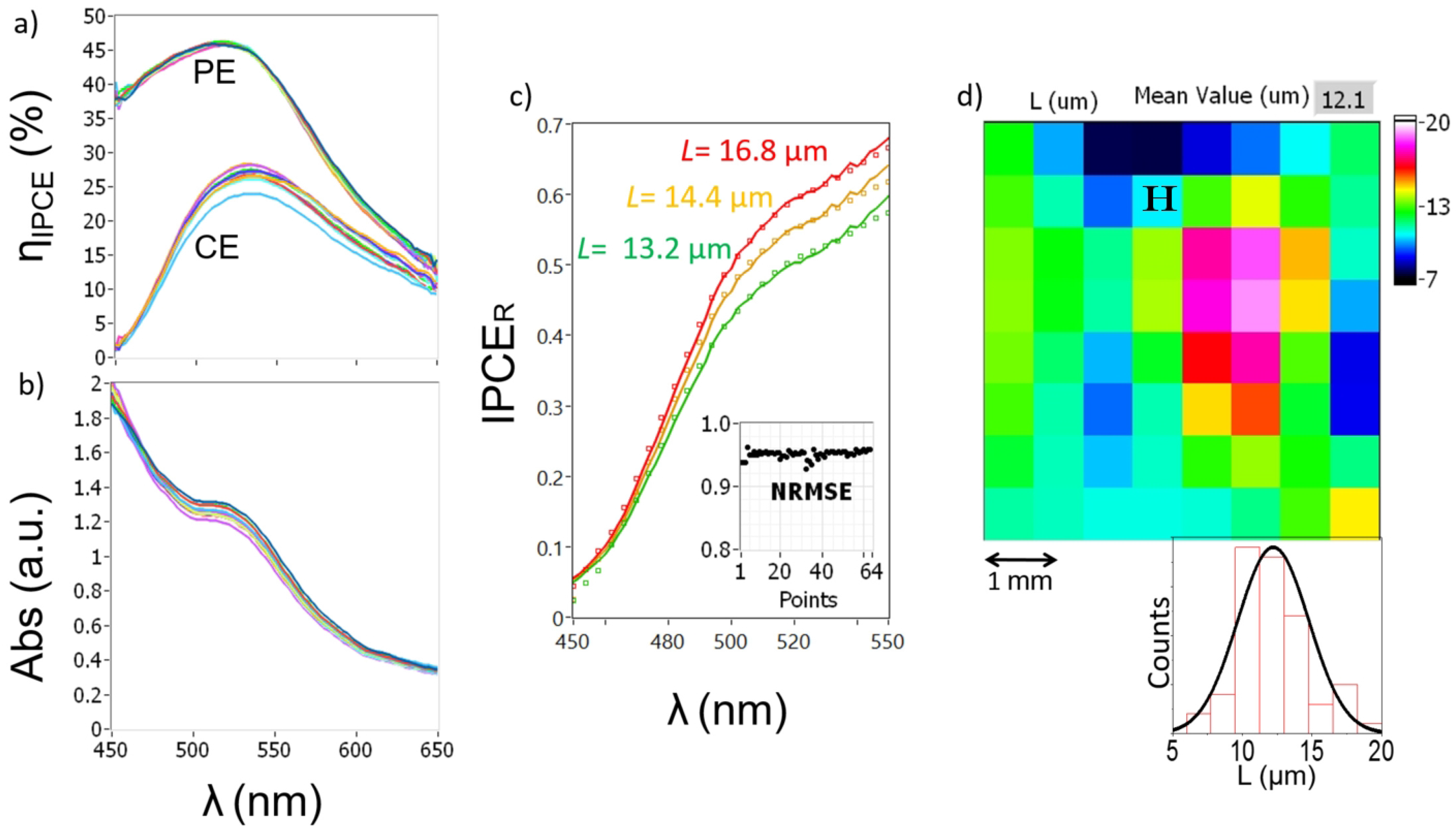
The spectral range between 450 nm and 650 nm with 2 nm of resolution was investigated. Underestimation of the IPCE values [41,42] was avoided by modulating the monochromatic beam at 0.33 Hz with an integration time of 10 s, resulting in a total acquisition period of 7.1 h for one side of the cell. This is responsible for the higher absolute values of ${\mathsf{\eta }}_{IPCE}$ compared to the high resolution scan (Figure 5b,c). Figure 6a,b shows the $IPC{E}_{\text{PE}}$, $IPC{E}_{\text{CE}}$ and absorbance spectra that show an evident variation of $IPC{E}_{\text{CE}}$ and absorbance. $IPC{E}_{\text{R}}$ spectrum fittings are performed between 450 nm and 550 nm in order to minimize the sensitivity of L. For clarity, only three spatial points have been chosen to highlight the fitting results (Figure 6c). The normalized root mean square (NRMS) error for each point is plotted in the inset showing an average value of 0.95 that confirms the goodness of fit. The resulting diffusion length map (Figure 6d) reports an increase up to 19 $\mathsf{\mu }$m located in the center of the device and several points with values lower than the film thickness (d = 11 $\mathsf{\mu }$m). The histogram reports an average value of 12.1 $\mathsf{\mu }$m that confirms the low ${\mathsf{\eta }}_{IPCE}$ recorded on the device.

The estimated $L(x,y)$ can be used to readily calculate ${\mathsf{\eta }}_{\text{col}}$ spectra from Equations (9) and (10) leaving ${\mathsf{\eta }}_{\text{sep}}$ the only unknown parameter in Equation (2). As already reported by Halme et al. [34] and Jennings et al. [23], a second fitting procedure with the experimental ${\mathsf{\eta }}_{IPCE}$ for CE and PE illumination allows one to estimate the wavelength-dependent ${\mathsf{\eta }}_{\text{sep}}$. Figure 7a shows the experimental (dot) and fitted (line) of ${\mathsf{\eta }}_{IPCE}$ for a single spatial point (Point “H” reported on Figure 6d); the estimated ${\mathsf{\eta }}_{\text{sep}}$ is reported in Figure 7b already with the calculated ${\mathsf{\eta }}_{\text{col}}$ and ${\mathsf{\eta }}_{\text{LH}}$. The low ${\mathsf{\eta }}_{\text{sep}}$ and the short L values are the main causes of the poor performance of the device under investigation. Unfortunately, the strong wavelength dependence of ${\mathsf{\eta }}_{\text{sep}}$ cannot be uniquely associated with the injection or regeneration problems of the sensitizer; anyway, two causes can be hypothesized: a mismatch between the excited-state energy levels of the dye and the electron acceptor states in the TiO${}_2$ (injection process) [23] or/and a poor regeneration efficiency that results in a strong dependence of the regeneration process with light intensity or [46,47].

4.3. Estimation of L by Electrochemical Impedance Spectroscopy

The diffusion length value obtained by the $IPC{E}_{\text{R}}$ technique was compared with EIS data fitted with the equivalent circuit shown in Figure 1. Measurement was performed under the same homogeneous circumstances as for the IPCE test (red light illumination and open circuit condition). In order to improve the quality of the fitting, all of the capacitors were replaced by constant phase elements (CPE) with an exponent ranging from 0.85 to 0.99. Interestingly, the EIS spectrum reported in Figure 8 resembles that of a Gerischer impedance instead of a classic transmission line [14] that is necessary to evaluate $R_{\text{ct}}$ and $R_{\text{t}}$. However, as already demonstrated [23,34], the transmission line model can still be adopted for $L>d/2$. In this study, a slightly higher value of L (15.1 $\mathsf{\mu }$m) with respect to the SATEM analysis is obtained. This result confirms the potentiality of the SATEM technique to map the distribution of the diffusion length over the sample accurately.

5. Materials and Methods

A 0.25 cm${}^2$ active area cell was fabricated with transparent nanoporous TiO${}_2$ paste (DSL 18NR-T) from Dyesol screen-printed through a 43T mesh screen onto fluorine-doped tin oxide (FTO)-coated glass substrate (NSG TEC 8/from Pilkington Group Limited, St Helens, UK). After 15 min of drying at 80 ${}^{\circ }$C, TiO${}_2$ films were sintered at 525 ${}^{\circ }$C for 30 min. The resulting thickness of the TiO${}_2$ films was measured with a surface profilometer Dektak 150 from Veeco and was observed to be 6.7 $\mathsf{\mu }$m. TiO${}_2$ electrodes were dyed for 16 h in a 0.3 mM solution of Z907 from Dyesol. After dyeing, the PEs were rinsed with ethanol in order to remove the excess dye before the assembling process. Platinized CEs were made by screen-printing platinum paste through a 100T mesh screen onto FTO-coated glass substrate. The CEs were dried at 80 ${}^{\circ }$C and then sintered at 525 ${}^{\circ }$C for 30 min. The two electrodes were laminated with Bynel from Solaronix (Aubonne, Switzerland). After the hot-melting step, the distance between the two electrodes was measured to be about 45 $\mathsf{\mu }$m. The used electrolyte was a commercial iodine-based electrolyte HSE from Dyesol.

6. Conclusions

SATEM is the first scanning apparatus that implements the steady state $IPC{E}_R$ technique under homogeneous conditions for an indirect estimation of the diffusion length in a DSC. The current study is believed to give insight into the system design and analytic procedure for reliable estimates of spatially-resolved L. The homogeneous conditions are the main peculiarity of the technique. In particular, $IPC{E}_{\text{PE}}$, $IPC{E}_{\text{CE}}$ and absorbance spectra were acquired with uniform background generation (bias light at 625 nm) and uniform background electron density (open circuit voltage). We highlighted the most delicate parameters through a depth sensitivity analysis of L; in particular, the high value of the sensitivity with respect to the film thickness ($S_d^L$) has been mitigated by increasing the optical spot size to 650 $\mathsf{\mu }$m, resulting in a lower spatial resolution of the L distribution. This point can be easily improved by arranging an experimental $d(x,y)$ with a profilometer measurement over the photoanode instead of the average value. Moreover, a better design of the optical line will give more room of improvement. Good agreement was obtained with the integral value of L estimated by an EIS analysis under the same operative conditions, confirming the remarkable setting of SATEM analysis. We believe that these results provide a solid base to extend the technique to different semi-transparent technologies, such as perovskite-based cells [48,49,50] and organic cells [51,52,53]). Unfortunately, a role in transport and recombination can be played by other contributions (for instance drift) that may have to be taken into account for precise collection efficiency modeling [54,55]. However, it has been demonstrated that the electric field contribution in organic solar cells arises mainly at a high level of irradiation (1 sun) as a consequence of a charge accumulation in the device [56], and we suppose it to be negligible in our experimental conditions. In perovskite solar cells, a recent article [57] demonstrated the field free condition of the methyl-ammonium lead iodide (MAPI) layer under short and open circuit conditions; moreover, as already assumed in several works [58,59,60], we believe that a diffusion-based transport model could be a starting point for an investigation with the SATEM analysis. Further research is required in this direction to unravel the limiting mechanisms of the IPCE and optical-based analysis for the extraction of the charge collection capabilities of hybrid-organic solar cells.

References

- Chen, W.; Nikiforov, M.P.; Darling, S.B. Morphology characterization in organic and hybrid solar cells. Energy Environ. Sci. 2012, 5, 8045–8074. [Google Scholar] [CrossRef]
- Pfannmoller, M.; Kowalsky, W.; Schroder, R.R. Visualizing physical, electronic, and optical properties of organic photovoltaic cells. Energy Environ. Sci. 2013, 6, 2871–2891. [Google Scholar] [CrossRef]
- Fakharuddin, A.; Jose, R.; Brown, T.M.; Fabregat-Santiago, F.; Bisquert, J. A roadmap for dye-sensitized solar modules. Energy Environ. Sci. 2014, 7, 3952–3981. [Google Scholar] [CrossRef]
- Asghar, M.I.; Miettunen, K.; Halme, J.; Vahermaa, P.; Toivola, M.; Aitola, K.; Lund, P. Review of stability for advanced dye solar cells. Energy Environ. Sci. 2010, 3, 418–426. [Google Scholar] [CrossRef]
- Gao, Y.; Martin, T.P.; Thomas, A.K.; Grey, J.K. Resonance Raman spectroscopic- and photocurrent imaging of polythiophene/fullerene solar cells. J. Phys. Chem. Lett. 2010, 1, 178–182. [Google Scholar] [CrossRef]
- Gao, Y.; Martin, T.P.; Niles, E.T.; Wise, A.J.; Thomas, A.K.; Grey, J.K. Understanding morphology-dependent polymer aggregation properties and photocurrent generation in polythiophene/fullerene solar cells of variable compositions. J. Phys. Chem. C 2010, 114, 15121–15128. [Google Scholar] [CrossRef]
- Brenner, T.J.K.; McNeill, C.R. Spatially resolved spectroscopic mapping of photocurrent and photoluminescence in polymer blend photovoltaic devices. J. Phys. Chem. C 2011, 115, 19364–19370. [Google Scholar] [CrossRef]
- Bokalič, M.; Topič, M. Spatially Resolved Characterization in Thin-Film Photovoltaics; Springer: Cham, Switzerland, 2015. [Google Scholar]
- Marek, J. Light-beam-induced current characterization of grain boundaries. J. Appl. Phys. 1984, 55, 318–326. [Google Scholar] [CrossRef]
- Carstensen, J.; Popkirov, G.; Bahr, J.; Föll, H. CELLO: An advanced LBIC measurement technique for solar cell local characterization. Sol. Energy Mater. Sol. Cells 2003, 76, 599–611. [Google Scholar] [CrossRef]
- Junghänel, M.; Tributsch, H. Monitoring the reactivity of oxide interfaces in dye solar cells with photocurrent imaging techniques. Comptes R. Chim. 2006, 9, 652–658. [Google Scholar] [CrossRef]
- Bokalič, M.; Krašovec, U.O.; Topič, M. Electroluminescence as a spatial characterisation technique for dye-sensitised solar cells. Prog. Photovolt. Res. Appl. 2013, 21, 1176–1180. [Google Scholar] [CrossRef]
- Raj, C.C.; Prasanth, R. A critical review of recent developments in nanomaterials for photoelectrodes in dye sensitized solar cells. J. Power Sources 2016, 317, 120–132. [Google Scholar] [CrossRef]
- Halme, J.; Vahermaa, P.; Miettunen, K.; Lund, P. Device physics of dye solar cells. Adv. Mater. 2010, 22, E210–E234. [Google Scholar] [CrossRef] [PubMed]
- Hagfeldt, A.; Boschloo, G.; Sun, L.; Kloo, L.; Pettersson, H. Dye-sensitized solar cells. Chem. Rev. 2010, 110, 6595–6663. [Google Scholar] [CrossRef] [PubMed]
- Ye, M.; Wen, X.; Wang, M.; Iocozzia, J.; Zhang, N.; Lin, C.; Lin, Z. Recent advances in dye-sensitized solar cells: From photoanodes, sensitizers and electrolytes to counter electrodes. Mater. Today 2015, 18, 155–162. [Google Scholar] [CrossRef]
- Fabregat-Santiago, F.; Bisquert, J.; Cevey, L.; Chen, P.; Wang, M.; Zakeeruddin, S.M.; Grätzel, M. Electron transport and recombination in solid-state dye solar cell with spiro-OMeTAD as hole conductor. J. Am. Chem. Soc. 2009, 131, 558–562. [Google Scholar] [CrossRef] [PubMed]
- Navas, J.; Guillen, E.; Alcantara, R.; Fernandez-Lorenzo, C.; Martin-Calleja, J.; Oskam, G.; Idigoras, J.; Berger, T.; Anta, J.A. Direct estimation of the electron diffusion length in dye-sensitized solar cells. J. Phys. Chem. Lett. 2011, 2, 1045–1050. [Google Scholar] [CrossRef]
- Park, J.K.; Kang, J.C.; Kim, S.Y.; Son, B.H.; Park, J.Y.; Lee, S.; Ahn, Y.H. Diffusion length in nanoporous photoelectrodes of dye-sensitized solar cells under operating conditions measured by photocurrent microscopy. J. Phys. Chem. Lett. 2012, 3, 3632–3638. [Google Scholar] [CrossRef] [PubMed]
- Dunn, H.K.; Westin, P.O.; Staff, D.R.; Peter, L.M.; Walker, A.B.; Boschloo, G.; Hagfeldt, A. Determination of the electron diffusion length in dye-sensitized solar cells by substrate contact patterning. J. Phys. Chem. C 2011, 115, 13932–13937. [Google Scholar] [CrossRef] [Green Version]
- Barnes, P.R.F.; Liu, L.; Li, X.; Anderson, A.Y.; Kisserwan, H.; Ghaddar, T.H.; Durrant, J.R.; O’Regan, B.C. Re-evaluation of recombination losses in dye-sensitized cells: The failure of dynamic relaxation methods to correctly predict diffusion length in nanoporous photoelectrodes. Nano Lett. 2009, 9, 3532–3538. [Google Scholar] [CrossRef] [PubMed]
- Barnes, P.R.; Anderson, A.Y.; Koops, S.E.; Durrant, J.R.; O’Regan, B.C. Electron injection efficiency and diffusion length in dye-sensitized solar cells derived from incident photon conversion efficiency measurements. J. Phys. Chem. C 2008, 113, 1126–1136. [Google Scholar] [CrossRef]
- Jennings, J.R.; Li, F.; Wang, Q. Reliable determination of electron diffusion length and charge separation efficiency in dye-sensitized solar cells. J. Phys. Chem. C 2010, 114, 14665–14674. [Google Scholar] [CrossRef]
- Agresti, A.; Cinà, L.; Pescetelli, S.; Taheri, B.; Di Carlo, A. Stability of dye-sensitized solar cell under reverse bias condition: Resonance Raman spectroscopy combined with spectrally resolved analysis by transmittance and efficiency mapping. Vib. Spectrosc. 2016, 84, 106–117. [Google Scholar] [CrossRef]
- Soedergren, S.; Hagfeldt, A.; Olsson, J.; Lindquist, S.E. Theoretical models for the action spectrum and the current-voltage characteristics of microporous semiconductor films in photoelectrochemical cells. J. Phys. Chem. 1994, 98, 5552–5556. [Google Scholar] [CrossRef]
- Wang, H.; Peter, L.M. A comparison of different methods to determine the electron diffusion length in dye-sensitized solar cells. J. Phys. Chem. C 2009, 113, 18125–18133. [Google Scholar] [CrossRef]
- Fabregat-Santiago, F.; Bisquert, J.; Garcia-Belmonte, G.; Boschloo, G.; Hagfeldt, A. Influence of electrolyte in transport and recombination in dye-sensitized solar cells studied by impedance spectroscopy. Sol. Energy Mater. Sol. Cells 2005, 87, 117–131. [Google Scholar] [CrossRef]
- Fabregat-Santiago, F.; Bisquert, J.; Palomares, E.; Otero, L.; Kuang, D.; Zakeeruddin, S.M.; Grätzel, M. Correlation between photovoltaic performance and impedance spectroscopy of dye-sensitized solar cells based on ionic liquids. J. Phys. Chem. C 2007, 111, 6550–6560. [Google Scholar] [CrossRef]
- Garland, J.; Crain, D.; Roy, D. Utilization of electrochemical impedance spectroscopy for experimental characterization of the diode features of charge recombination in a dye sensitized solar cell. Electrochim. Acta 2014, 148, 62–72. [Google Scholar] [CrossRef]
- Bisquert, J. Theory of the impedance of electron diffusion and recombination in a thin layer. J. Phys. Chem. B 2002, 106, 325–333. [Google Scholar] [CrossRef]
- Jennings, J.R.; Wang, Q. Impedance spectroscopy of dye-sensitized solar cells: Analysis of measurement and fitting errors. J. Electrochem. Soc. 2012, 159, F141–F149. [Google Scholar] [CrossRef]
- Bisquert, J.; Mora-Sero, I. Simulation of steady-state characteristics of dye-sensitized solar cells and the interpretation of the diffusion length. J. Phys. Chem. Lett. 2010, 1, 450–456. [Google Scholar] [CrossRef]
- Fabregat-Santiago, F.; Garcia-Belmonte, G.; Bisquert, J.; Zaban, A.; Salvador, P. Decoupling of transport, charge storage, and interfacial charge transfer in the nanocrystalline TiO2/electrolyte system by impedance methods. J. Phys. Chem. B 2002, 106, 334–339. [Google Scholar] [CrossRef]
- Halme, J.; Boschloo, G.; Hagfeldt, A.; Lund, P. Spectral characteristics of light harvesting, electron injection, and steady-state charge collection in pressed TiO2 dye solar cells. J. Phys. Chem. C 2008, 112, 5623–5637. [Google Scholar] [CrossRef]
- Ansari-Rad, M.; Abdi, Y.; Arzi, E. Reaction order and ideality factor in dye-sensitized nanocrystalline solar cells: A theoretical investigation. J. Phys. Chem. C 2012, 116, 10867–10872. [Google Scholar] [CrossRef]
- Villanueva-Cab, J.; Wang, H.; Oskam, G.; Peter, L.M. Electron diffusion and back reaction in dye-sensitized solar cells: The effect of nonlinear recombination kinetics. J. Phys. Chem. Lett. 2010, 1, 748–751. [Google Scholar] [CrossRef] [Green Version]
- Xue, G.; Guo, Y.; Yu, T.; Guan, J.; Yu, X.; Zhang, J.; Liu, J.; Zou, Z. Degradation mechanisms investigation for long-term thermal stability of dye-sensitized solar cells. Int. J. Electrochem. Sci. 2012, 7, 1496–1511. [Google Scholar]
- Fisher, A.; Peter, L.; Ponomarev, E.; Walker, A.; Wijayantha, K. Intensity dependence of the back reaction and transport of electrons in dye-sensitized nanocrystalline TiO2 solar cells. J. Phys. Chem. B 2000, 104, 949–958. [Google Scholar] [CrossRef]
- Trupke, T.; Würfel, P.; Uhlendorf, I. Dependence of the photocurrent conversion efficiency of dye-sensitized solar cells on the incident light intensity. J. Phys. Chem. B 2000, 104, 11484–11488. [Google Scholar] [CrossRef]
- Peter, L.; Wijayantha, K. Intensity dependence of the electron diffusion length in dye-sensitised nanocrystalline TiO2 photovoltaic cells. Electrochem. Commun. 1999, 1, 576–580. [Google Scholar] [CrossRef]
- Xue, G.; Yu, X.; Yu, T.; Bao, C.; Zhang, J.; Guan, J.; Huang, H.; Tang, Z.; Zou, Z. Understanding of the chopping frequency effect on IPCE measurements for dye-sensitized solar cells: From the viewpoint of electron transport and extinction spectrum. J. Phys. D Appl. Phys. 2012, 45. [Google Scholar] [CrossRef]
- Tian, H.; Liu, L.; Liu, B.; Yuan, S.; Wang, X.; Wang, Y.; Yu, T.; Zou, Z. Influence of capacitance characteristic on dye-sensitized solar cell’s IPCE measurement. J. Phys. D Appl. Phys. 2009, 42. [Google Scholar] [CrossRef]
- Hishikawa, Y.; Yanagida, M.; Koide, N. Performance Characterization of the Dye-Sensitized Solar Cells. In Proceedings of the Conference Record of the Thirty-First IEEE Photovoltaic Specialists Conference, Lake Buena Vista, FL, USA, 3–7 January 2005; pp. 67–70.
- Yang, X.; Yanagida, M.; Han, L. Reliable evaluation of dye-sensitized solar cells. Energy Environ. Sci. 2013, 6, 54–66. [Google Scholar] [CrossRef]
- Chen, C.Y.; Pootrakulchote, N.; Hung, T.H.; Tan, C.J.; Tsai, H.H.; Zakeeruddin, S.M.; Wu, C.G.; Grätzel, M. Ruthenium sensitizer with thienothiophene-linked Carbazole Antennas in conjunction with liquid electrolytes for dye-sensitized solar cells. J. Phys. Chem. C 2011, 115, 20043–20050. [Google Scholar] [CrossRef]
- Li, F.; Jennings, J.R.; Wang, Q. Determination of sensitizer regeneration efficiency in dye-sensitized solar cells. ACS Nano 2013, 7, 8233–8242. [Google Scholar] [CrossRef] [PubMed]
- Li, F.; Jennings, J.R.; Wang, X.; Fan, L.; Koh, Z.Y.; Yu, H.; Yan, L.; Wang, Q. Influence of ionic liquid on recombination and regeneration kinetics in dye-sensitized solar cells. J. Phys. Chem. C 2014, 118, 17153–17159. [Google Scholar] [CrossRef]
- Eperon, G.E.; Burlakov, V.M.; Goriely, A.; Snaith, H.J. Neutral color semitransparent microstructured perovskite solar cells. ACS Nano 2014, 8, 591–598. [Google Scholar] [CrossRef] [PubMed]
- Roldan-Carmona, C.; Malinkiewicz, O.; Betancur, R.; Longo, G.; Momblona, C.; Jaramillo, F.; Camacho, L.; Bolink, H.J. High efficiency single-junction semitransparent perovskite solar cells. Energy Environ. Sci. 2014, 7, 2968–2973. [Google Scholar] [CrossRef]
- Guo, F.; Azimi, H.; Hou, Y.; Przybilla, T.; Hu, M.; Bronnbauer, C.; Langner, S.; Spiecker, E.; Forberich, K.; Brabec, C.J. High-performance semitransparent perovskite solar cells with solution-processed silver nanowires as top electrodes. Nanoscale 2015, 7, 1642–1649. [Google Scholar] [CrossRef] [PubMed]
- Pastorelli, F.; Romero-Gomez, P.; Betancur, R.; Martinez-Otero, A.; Mantilla-Perez, P.; Bonod, N.; Martorell, J. Enhanced light harvesting in semitransparent organic solar cells using an optical metal cavity configuration. Adv. Energy Mater. 2015, 5. [Google Scholar] [CrossRef]
- Ren, X.; Li, X.; Choy, W.C. Optically enhanced semi-transparent organic solar cells through hybrid metal/nanoparticle/dielectric nanostructure. Nano Energy 2015, 17, 187–195. [Google Scholar] [CrossRef]
- Liu, Z.; You, P.; Liu, S.; Yan, F. Neutral-color semitransparent organic solar cells with all-graphene electrodes. ACS Nano 2015, 9, 12026–12034. [Google Scholar] [CrossRef] [PubMed]
- Pivrikas, A.; Sariciftci, N.S.; Juška, G.; Österbacka, R. A review of charge transport and recombination in polymer/fullerene organic solar cells. Prog. Photovolt. Res. Appl. 2007, 15, 677–696. [Google Scholar] [CrossRef]
- Tress, W.; Leo, K.; Riede, M. Optimum mobility, contact properties, and open-circuit voltage of organic solar cells: A drift-diffusion simulation study. Phys. Rev. B 2012, 85. [Google Scholar] [CrossRef]
- Hwang, I.; McNeill, C.R.; Greenham, N.C. Drift-diffusion modeling of photocurrent transients in bulk heterojunction solar cells. J. Appl. Phys. 2009, 106. [Google Scholar] [CrossRef]
- Bergmann, V.W.; Guo, Y.; Tanaka, H.; Hermes, I.M.; Li, D.; Klasen, A.; Bretschneider, S.A.; Nakamura, E.; Berger, R.; Weber, S.A.L. Local time-dependent charging in a perovskite solar cell. ACS Appl. Mater. Interfaces 2016, 8, 19402–19409. [Google Scholar]
- Guillen, E.; Ramos, F.J.; Anta, J.A.; Ahmad, S. Elucidating transport-recombination mechanisms in perovskite solar cells by small-perturbation techniques. J. Phys. Chem. C 2014, 118, 22913–22922. [Google Scholar] [CrossRef]
- Stranks, S.D.; Eperon, G.E.; Grancini, G.; Menelaou, C.; Alcocer, M.J.P.; Leijtens, T.; Herz, L.M.; Petrozza, A.; Snaith, H.J. Electron-hole diffusion lengths exceeding 1 micrometer in an organometal trihalide perovskite absorber. Science 2013, 342, 341–344. [Google Scholar] [PubMed]
- Minemoto, T.; Murata, M. Device modeling of perovskite solar cells based on structural similarity with thin film inorganic semiconductor solar cells. J. Appl. Phys. 2014, 116. [Google Scholar] [CrossRef]
Figure 1.
Small signal equivalent circuit of dye-sensitized solar cells (DSCs) used to fit electrochemical impedance spectroscopy (EIS) spectra. The transmission line is outlined by the red box; and are discussed in the main text. The model includes also: distributed capacitance of TiO (), series resistor (), charge-transfer resistance () and double-layer capacitance () at the exposed transparent conducting oxide (TCO)-electrolyte interface, resistor () and capacitor () at the interface, Warburg element () for Nernst diffusion of in the electrolyte, charge-transfer resistance () and double-layer capacitance () at the platinized counter-electrode.
Figure 2.
Optical layer structure of a typical DSC. PE: photo electrode; and CE: counter electrode.
Figure 3.
Illustration of the set up.
Figure 4.
sensitivity functions with respect to , d, , and . For , and , we have set 11 m, 21 m and assumed a typical film reflectance spectra.
Figure 5.
(a) Photo of the DSC with 0.25 cm of active area. Spatial maps of (b) , (c) and (d) absorbance acquired at 530 nm.
Figure 6.
(a,b) and and absorbance spectra of 64 spatial points of the active area; (c) fitting results from 450 nm and 550 nm (points are experimental values) of three spatial points. The normalized root mean square (NRMS) error for each point is plotted in the inset, showing an average value of 0.95 that confirms the goodness of fit. (d) Spatial map of the estimated L; the normal distribution reported below shows an average value of 12.1 m.
Figure 7.
(a) Fitting of the and by varying the spectrum for Point “H” of Figure 6d. (b) Estimated and calculated light harvesting and collection efficiencies for the both the PE and the CE side.
Figure 8.
Impedance spectra under the open circuit condition (0.51 V). Fitting was achieved using the model shown in Figure 1 with an extracted diffusion length of 15.1 m.
© 2016 by the authors; licensee MDPI, Basel, Switzerland. This article is an open access article distributed under the terms and conditions of the Creative Commons Attribution (CC-BY) license (http://creativecommons.org/licenses/by/4.0/).
Share and Cite
MDPI and ACS Style
Cinà, L.; Taheri, B.; Reale, A.; Di Carlo, A. Diffusion Length Mapping for Dye-Sensitized Solar Cells. Energies 2016, 9, 686. https://doi.org/10.3390/en9090686
AMA Style
Cinà L, Taheri B, Reale A, Di Carlo A. Diffusion Length Mapping for Dye-Sensitized Solar Cells. Energies. 2016; 9(9):686. https://doi.org/10.3390/en9090686
Chicago/Turabian StyleCinà, Lucio, Babak Taheri, Andrea Reale, and Aldo Di Carlo. 2016. "Diffusion Length Mapping for Dye-Sensitized Solar Cells" Energies 9, no. 9: 686. https://doi.org/10.3390/en9090686
Note that from the first issue of 2016, this journal uses article numbers instead of page numbers. See further details here.