Enhanced Forecasting Approach for Electricity Market Prices and Wind Power Data Series in the Short-Term

Abstract

The uncertainty and variability in electricity market price (EMP) signals and players’ behavior, as well as in renewable power generation, especially wind power, pose considerable challenges. Hence, enhancement of forecasting approaches is required for all electricity market players to deal with the non-stationary and stochastic nature of such time series, making it possible to accurately support their decisions in a competitive environment with lower forecasting error and with an acceptable computational time. As previously published methodologies have shown, hybrid approaches are good candidates to overcome most of the previous concerns about time-series forecasting. In this sense, this paper proposes an enhanced hybrid approach composed of an innovative combination of wavelet transform (WT), differential evolutionary particle swarm optimization (DEEPSO), and an adaptive neuro-fuzzy inference system (ANFIS) to forecast EMP signals in different electricity markets and wind power in Portugal, in the short-term, considering only historical data. Test results are provided by comparing with other reported studies, demonstrating the proficiency of the proposed hybrid approach in a real environment.

1. Introduction

In competitive and deregulated electricity markets, potential integration of renewables, especially wind power, which naturally introduces its stochastic, volatile, and uncertain behaviour, is totally reflected in the market players’ strategies and presents more difficulties for a sustainable and robust management of the power framework. Even more when the renewable potential is introduced very widely, yielding higher production costs, inflexibility, and unnecessary penalties due to wrong strategies by players or an increment in emissions caused by conventional producers filling the gaps, especially when the renewable resources suddenly fail or do not cover the required demand [1]. Moreover, with the growing need for smart grids, for example to meet the growing interest in electric vehicles and their integration, the above concerns may be even more pronounced without the use of innovative tools or mechanisms to ensure the quality, safety, and robustness of the electrical system [2].

One of the approaches discussed nowadays in the scientific domain to mitigate some of the problems described above and to achieve a profitable and sustainable management of the electrical framework involves the integration of energy storage systems, which makes the electrical system more flexible due to the increased exploitation of potential usage of renewables, especially under peak loads, reducing the operational cost or curtailment events; however their implementation is still highly costly and in experimental phases in some cases [3].

An alternative way to tackle the aforementioned concerns in power systems and in competitive electricity markets, which are by nature more economical and useful for all agent players, is through the use of innovative forecasting tools to determine the future behaviour of the renewable potential or electricity market price (EMP) signals; making the creation of sets of possible market strategies suitable, considering other important indicators such as social behaviour, environmental factors, electrical constraints, and the behaviours of other electricity agents; in other words, the forecasting tools may be used as a first stage of defense for all market players [4]. In the last years, massive efforts, supported by the scientific community, have been made to propose more viable and reliable solutions, allowing mitigation of the countless concerns regarding power systems, which are reflected in widespread techniques and forecasting approaches for EMPs or wind power behaviour, considering statistical or physical models in soft or hard computing, as shown for instance in [5,6,7], considering very short-, short-, and long-term horizon forecasting [8,9].

Regarding EMP forecasting tools, since 2005, models such as autoregressive integrated moving average (ARIMA) combined with wavelet transform (WT) [10] can be found. This model belongs to the family of hard computing tools, which require a large amount of physical information and an exact modelling of the system, resulting in high computational complexity, and in this sense, will not be considered in this review of the state of the art. However, soft computing models, such as fuzzy neural network (FNN) [11] or hybrid intelligent system (HIS) [12], are among the soft computing models, which require the usage of any auto learning process from historical sets to identify future patterns and therefore require less computational complexity or information to model the problem. In this regard, several examples can be found such as neural network (NN) models [13], adaptive wavelet NN (AWNN) [14], cascaded neuro-evolutionary algorithm (CNEA) [15], cascaded NN (CNN) [16], the hybrid neuro-evolutionary system (HNES) [17], and some hybrid forecasting models, such as those presented in [18], or a combination of WT with particle swarm optimization (PSO) and the adaptive neuro-fuzzy inference system (ANFIS) (WPA) [19] and other hybrids [20], the hybrid fundamental-econometric model [21], or two-stage approaches such as those reported in [22,23]. Furthermore, more approaches considering singular spectrum analysis [24], informative vector machine [25], or even new genetic algorithms such as Levenberg-Marquardt and cuckoo search algorithms [26] and genetic regression of relevance vector machines [27] can be found for different EMP prices analyses, considering the Spanish, Pennsylvania-New Jersey-Maryland (PJM), Australian National Electricity Market (ANEM), and other liberalized electricity markets around the world as real case studies.

In wind power forecasting, widespread use of forecasting models for the very short and short term can be found in specialized literature considering soft computing and statistical models. In this sense, several examples are usually found, such as an evolutionary algorithm using an artificial intelligence model [28], NN [29,30], ridgelet NN [31], hybrid approaches composed of WT and a neuro-fuzzy network (NF) [32], WT with NN [33], WT with ANFIS (WNF) [34], or WPA [35]. Also, wind power forecasting can be tackled by considering a combination of WT with support vector machine (SVM) and statistical analysis [36], adaptive WT combined with feed-forward NN (AWNN) [37], WT combined with ARTMAP [38], and optimized SVM using a genetic algorithm [39]. More recently some proposals have considered a principal component analysis algorithm [40], hybrid WT, PSO, and NN [41], multi-layer artificial NN improved with simplified swarm optimization [42], and WT combined with NN, trained by an improved clonal selection algorithm [43]. All of the aforementioned models were run considering real cases with data from wind farms or historical data collected from the public domain in different locations around the world.

In this paper, in accordance with the features demonstrated by hybrid forecasting models briefly presented above, a new approach to forecast the EMP or wind power performance in the short term (from a few to 168 h ahead) is proposed.

Specifically, in the case of EMP forecasting, the proposed approach will perform a forecast for the next 168 h ahead with a time step of 1 h, considering only historical data available from the public domain, without considering the inclusion of exogenous data such as load and other energy prices, among others, to allow a fair and clean comparison with other already published methodologies. In the case of wind power forecasting, the proposed forecasting approach will perform the forecasting for a range of 3 h ahead with a time-step of 15 min, refreshing the system (input data and forecast results) until completion of the forecasting results for 24 h ahead. As in the previous case study, in wind power forecasting the proposed approach does not consider the inclusion of exogenous data such as wind profile and atmospheric data, among others, in order to make a fair and clean comparison with previously published approaches.

Furthermore, the proposed approach is composed of an innovative combination of WT as the pre-processing tool, which provides a smoothing effect of all inputs, providing more flexibility and more convergence to forecast the future behaviour, differential evolutionary particle swarm optimization (DEEPSO), which is itself a hybrid method and will be responsible for augmenting the performance of ANFIS (which is by nature a hybrid tool) by tuning the ANFIS membership functions to attain a lower forecasting error. Finally, the inverse WT will be used to introduce again the smoothing information collected at the beginning, providing the final forecasting signal. In this sense, hereafter the proposed approach will be called the hybrid WT+DEEPSO+ANFIS (HWDA) approach. In all case studies, the real historical data used will be comparable to those data used in reported and published models [44,45]. The remainder of the manuscript is organized as follows: Section 2 describes the concepts used to create the HWDA approach, the algorithm used for EMP or wind power forecasting, and the criteria used to validate and compare the capabilities of the proposed HWDA approach with previous and published methodologies. Section 3 describes the historical data used to carry out the forecasting considering the EMP or wind power, the detailed results, and the comparison carried out; finally, Section 4 presents the main conclusions drawn in this paper.

2. Proposed Approach

The HWDA approach results from the successful combination of WT, DEEPSO, and ANFIS. The WT is employed as a pre-processing step to decompose the historical sets of EMP or wind power into new constitutive sets with better behaviour. Then, the forthcoming values of those constitutive sets are the feeding sets of ANFIS responsible for creating the forecast results. DEEPSO augments the performance of ANFIS by tuning the ANFIS membership functions, resulting in lower forecasting error. In comparison with its ancestor, evolutionary particle swarm optimization (EPSO), the underlying evolutionary and differential concepts make real differences in terms of robustness, convergence, and computational time. So the combination of DEEPSO features with the adaptive characteristics of ANFIS means that they complement each other in positive way. Finally, the inverse WT is used to reconstruct the forecasting signal, and thus the final forecasting results are obtained.

2.1. Wavelet Transform

As reported in most of the previously described works on the state of the art, the application of WT in forecasting approaches is important for overcoming the limitations of non-stationary time series such as EMP or wind power; however, it may be applied in other engineering fields, since it enables the analysis of time series in their natural state. WT is used as a pre-processing tool for understanding non-stationary or time varying data [46], with sensibility to the irregularities of input data. In this sense, WT is especially useful for showing different aspects that constitute the data without losing the real signal content [47]. Despite the problems related with continuous WT (CWT) analysis, discrete WT (DWT) was created to give, in an effective way, a description relative to CWT, which is widely used to decompose the time series under study:

$$DWT\left(m_{wt},n_{wt}\right)=2^{-(m_{wt}/2)}{\displaystyle \sum }_{h=0}^{H}p\left(t_{wt}\right)\phi \left(\frac{t_{wt}-b}{a}\right)$$

(1)

where $H$ represents the length $p\left(t_{wt}\right)$, and the parameters of scaling ($a$) and translation ($b$) are changed to integer variables $a_{wt}=2^{m_{wt}}$ and $b_{wt}=n_{wt}{2}^{m_{wt}}$ respectively, with a time-step $t_{wt}$, i.e.,:

$$DWT\left(m_{wt},n_{wt}\right)=2^{-(m_{wt}/2)}{\displaystyle \sum }_{h=0}^{H}p\left(t_{wt}\right)\phi \left(\frac{t_{wt}-n_{wt}{2}^{m_{wt}}}{2^{m_{wt}}}\right)$$

(2)

The DWT is performed by multi-resolution analysis, where a “father wavelet”, responsible for the low-frequency series, is used with a complementary “mother wavelet”, which is responsible for the high-frequency series components [38]. In this paper and following the description cited in [44,45] the Daubechies of fourth order, or Db4, was used as the mother-wavelet function. The Db4 has asymmetrical and continuous proprieties, where a higher order level will create a higher level oscillation, which is desirable in forecasting [38,47]. The coefficients of approximations $A_n$ and details $D_n$ are expressed as:

$$A_n={\displaystyle \sum }_{n}DWT\left(m_{wt},n_{wt}\right){\phi }_{mn}\left(t\right)$$

(3)

$$D_n={\displaystyle \sum }_{n}DWT\left(m_{wt},n_{wt}\right){\psi }_{mn}\left(t\right)$$

(4)

where ${\phi }_{mn}\left(t_{wt}\right)$ is the father-wavelet and ${\psi }_{mn}\left(t_{wt}\right)$ is the mother-wavelet, and $DWT\left(m_{wt},n_{wt}\right)$ are the coefficients obtained from Equation (2) [33]. Furthermore, the Db4 is chosen as the mother-wavelet function due to a better trade-off between smoothness and length [19]. Also, the DWT used in this paper was created on four filters divided into two groups: the decomposition group, composed of low-pass and high-pass filters, and the reconstruction group, composed of low-pass and high-pass filters as described in [44,45]. Figure 1 shows a general decomposition model of WT, where approximation steps $A_n$ are able to analyse the universal information of original sets; that is, the low-frequency representation and description of the high-frequency component and the detailed steps $D_n$ are able to describe the difference between the successive approximations.

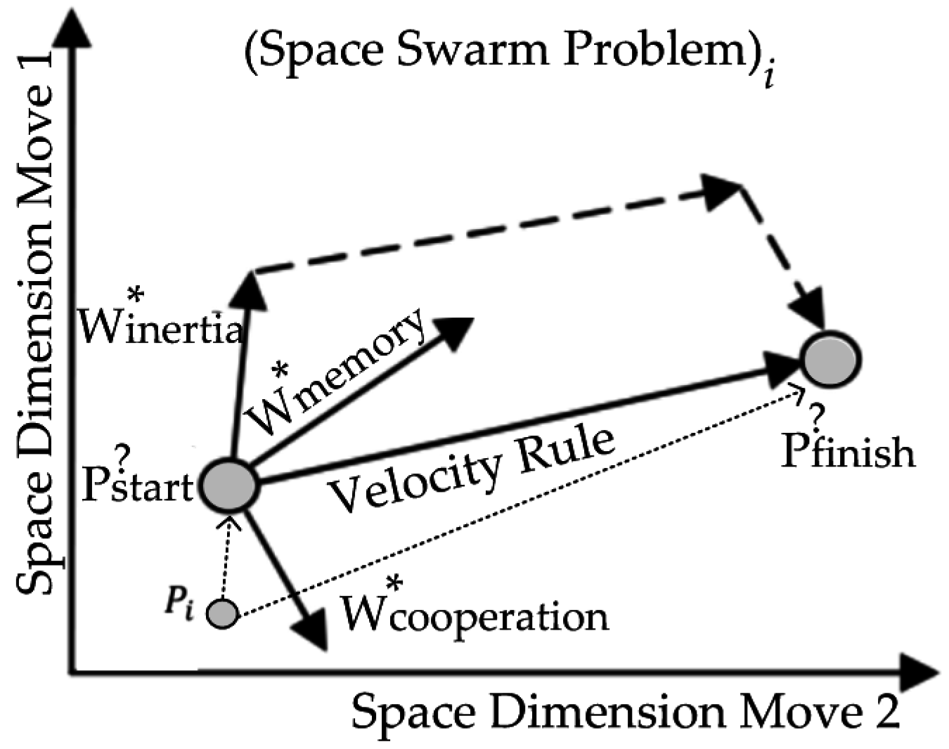
2.2. Differential Evolutionary Particle Swarm Optimization

DEEPSO is a successful hybrid combination of the EPSO model [44,45], which is itself a hybrid combination of its ancestor model, namely PSO, where weight factors have self-adaptive features, with evolutionary programming, which brings self-adaptive operators [48], and a differential evolution algorithm, which provides a new solution from the current particle of the swarm by adding a fraction difference between two other points found from the previously evaluated swarm [49]. The DEEPSO schema is similar to EPSO [50]; however, the movement rule Equation (6) has new notation:

$$X_i^{new}=X_i+V_i^{new}$$

(5)

$$V_i^{new}=w_{i0}^{*}{V}_i+w_{i1}^{*}\left(X_{r1}^i-X_{r2}^i\right)+P{w}_{i2}^{*}\left(b_g^{*}-X_i\right)$$

(6)

where the weights $w_{in-1}^{*}$ (inertia, memory and cooperation) are defined as:

$$w_{ik}^{*}=w_{ik}+\tau N\left(0,1\right)$$

(7)

and the global position is defined as:

$$b_g^{*}=b_g\left(1+w_{g}N\left(0,1\right)\right)$$

(8)

From Equation (6), components $X_r^i$ should be any pair of different particle already tested from the swarm, and ordered to minimize at the end of respective iteration, i.e.,:

$$f\left(X_{r1}^i\right)<f\left(X_{r2}^i\right)$$

(9)

From Equations (5)–(9), $X_i^{new}$ is the new position of the particle, $V_i^{new}$ is the new velocity found, $P$ is a diagonal binary matrix with a value of 1 when the probability is $p$ and 0 when the probability is $\left\{1-p\right\}$, $w_{ik}^{*}$ are the mutated weights of inertia, memory, and cooperation of the swarm, given by a learning parameter $\tau$ (fixed or mutated), and $N\left(0,1\right)$ is a random Gaussian variable with 0 mean and variance 1.

Also, $b_g^{*}$ is the global position provided by the new weight $w_g$, which is collected from a diagonal matrix, having a self-adaptive feature, and in this sense, it is a mutated element [48,49]. Components ${\mathrm{X}}_{\mathrm{r}1}^{\mathrm{i}}$ and ${\mathrm{X}}_{\mathrm{r}2}^{\mathrm{i}}$ guarantee that a suitable extraction really happens, considering macro-gradient points in a descending direction depending on the structured comparison of $f\left(X_{r1}^i\right)$ and $f\left(X_{r2}^i\right)$. In this sense, component $X_{r2}^i$ is assumed to be as $X_{r2}^i=X_i$, and component $X_{r1}^i$ is sampled from the set of best ancestors from the swarm of n particles, that is, $S_{bA}=\left\{b_1,b_2,\dots ,b_n\right\}$ [50,51,52]. The main idea underlying DEEPSO movement is briefly illustrated in Figure 2.

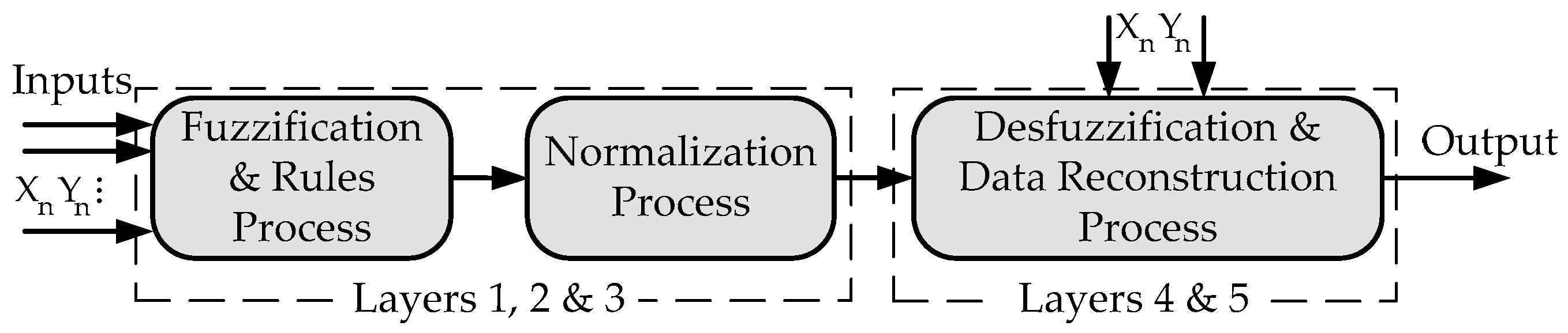
2.3. Adaptive Neuro-Fuzzy Inference System

ANFIS is a well-known hybrid combination of NN and fuzzy algorithms combining useful features such as low computational requirements, the possibility of dealing with a large number of data, and high response features. Furthermore, it has self-learning capabilities provided by the NN, which help it to self-adjust its parameters due to fuzzy capabilities [19,45]. The general ANFIS structure is based on several layers, which provide the fuzzification, rules, normalization data, desfuzzification, and data reconstruction process as described in [35,44]. Figure 3 briefly describes the multi-layer feed-forward network ANFIS structure. Mathematically, each of the five layers $l_{n_k}$ used is:

$$\{\begin{array}{c}{l}_{1_k}=\mu A_i\left(x\right),k=1,2\\ l_{1_k}=\mu B_{i-2}\left(y\right),k=3,4\end{array}$$

(10)

$$\mu A_k\left(x\right)=\frac{1}{1+{\left|\frac{x-r_k}{p_{ik}}\right|}^{2q_k}}$$

(11)

$$l_{2_k}=w_k=\mu A_k\left(x\right)\mu B_k\left(y\right),k=1,2$$

(12)

$$l_{3_k}={\overline{w}}_i=\frac{w_k}{w_1+w_2},k=1,2$$

(13)

$$l_{4_k}={\overline{w}}_k{z}_k={\overline{w}}_k\left(a_{k}x+b_{k}y+c_k\right),k=1,2$$

(14)

$$l_{5_k}={\displaystyle \sum }_k{\overline{w}}_k{z}_k=\frac{{\sum }_k{w}_k{z}_k}{{\sum }_k{w}_k}$$

(15)

From Equation (10), all nodes $k$ are adaptive nodes with node function $l_{1_k},$ where $x$ and $y$ are the input of the $k_{th}$ node and $A_k$ and $B_{k-2}$ are the membership function, also called the linguistic label, associated with these nodes. In this paper, a triangular membership function is normally used [44,45], where $\left\{p_k,q_k,r_k\right\}$ are parameter sets, because it is a continuous and piecewise differentiable function, described in $\text{Equation}\left(11\right)$, which represents the first layer. In Equation (12), all output nodes represent the firing strength of the rule $w_k$, where each node signal is multiplied by the previous inputs signals, representing the second layer. In Equation (13), the third layer, every node computes the ratio of firing strength rules ${\mathrm{k}}_{\text{th}}$ to the sum of all firing strength rules. Equation (14) represents the computation of all nodes’ contribution to $k_{th}$ rule with global output, where $\left\{a_k,b_k,c_k\right\}$ are parameter sets, and ${\overline{w}}_k$ is the layer output (fourth layer). Finally, Equation (15) defines the ANFIS output node, that is, the fifth layer where the summation Σ is made. As reported in [19,35], in this paper, the ANFIS structure follows the least-squares and back-propagation gradient descent method, considering the Takagi-Sugeno approach.

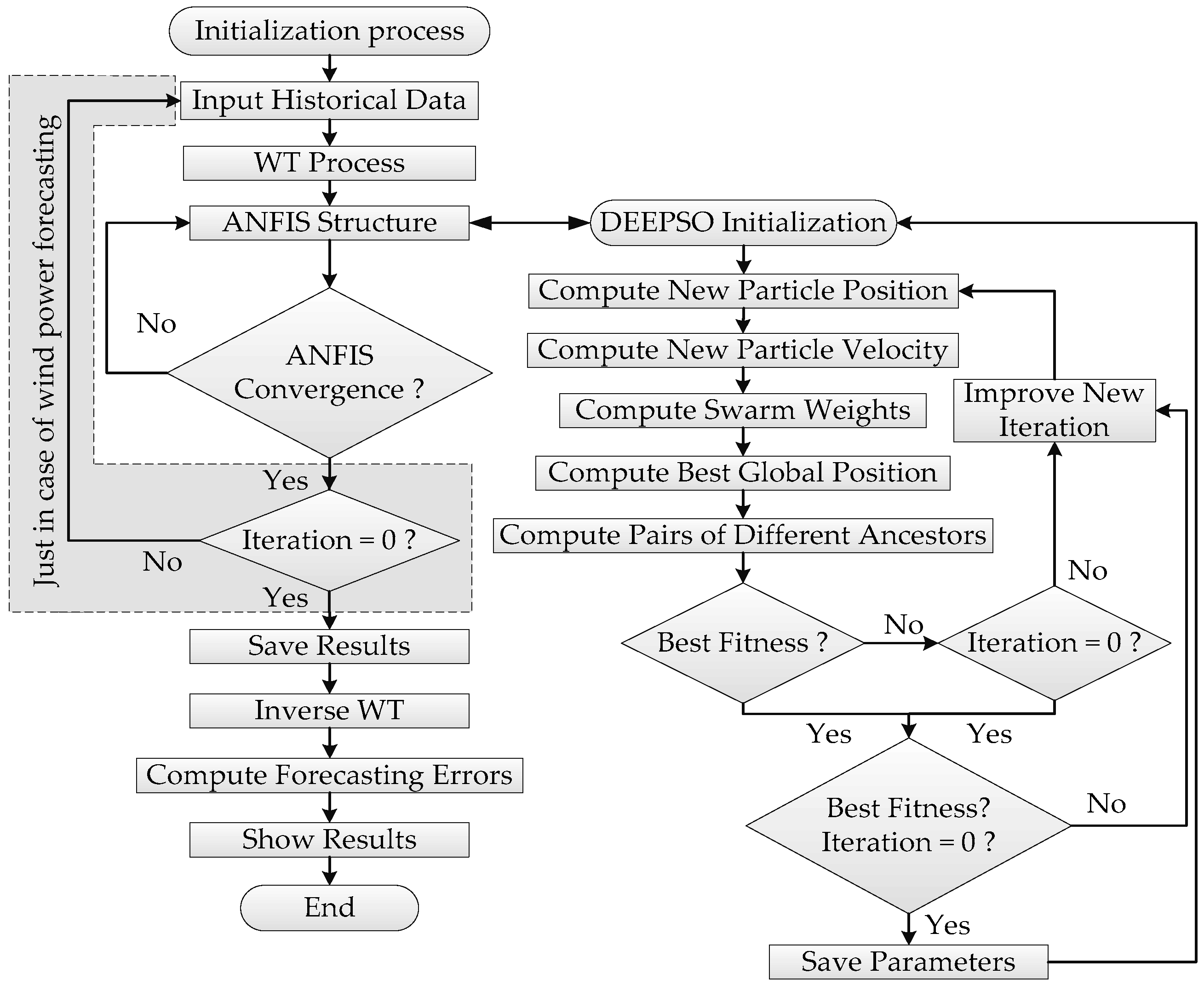
2.4. Hybrid Proposed Approach

As stated before, the HWDA approach results from a combination of WT, DEEPSO, and ANFIS. The WT is employed as a pre-processing step to decompose the historical sets. The DEEPSO augments the ANFIS performance by tuning the ANFIS membership functions. Finally, the inverse WT is used to reconstruct the forecasting signal, and then the final forecasting results are obtained. Figure 4 shows the HWDA flowchart. In detail, HWDA follows the following steps:

• Step 1: Initialize the HWDA approach with a historical data matrix of EMP or wind power, respectively, considering the forecasting time-scale of each forecast field;
• Step 2: Choose a set of historical data of the previous step to run the pre-processing process carried out by the WT tool. This step is performed by a backtracking process, in order to attain a smaller error at the end by choosing the best set of candidates. Also, the approach considered in this paper uses ${\mathrm{A}}_3$, ${\mathrm{D}}_3$, and ${\mathrm{D}}_1$ steps as inputs for the next step;
• Step 3: Train the ANFIS tool with the previous sets of constitutive historical data obtained from WT. The optimization process of the ANFIS membership function parameters will be achieved with the DEEPSO method. All parameters considered from all methods are summarized in

  Table 1. DEEPSO (differential evolutionary particle swarm optimization) and ANFIS (adaptive neuro-fuzzy inference system) parameters used for EMP (electricity market price) and wind power forecasting.

  Methods	Parameters	Type or Size
  WT	Decomposition Direction	Row
  	Level of Decomposition	3
  	Mother-Wavelet Function	Db4
  	Denoising Methods	“sqtwolog”–“minimaxi”
  	Multiplicative Thresholds Rescaling	“one”–“sln”
  DEEPSO	Communication Probability	0.10
  	Final Inertia Wight	0.01–0.15
  	Initial Inertia Weight	0.50–0.90
  	Initial Population Size	100
  	Initial Sharing Acceleration	0.50–2.00
  	Initial Swarm Learning Process	1.00–2.00
  	Initial Swarm Sharing Process	2.00
  	Learning Parameter	1
  	Maximum Value of New Position	Set of Max. Inputs
  	Minimum Value of New Position	Set of Min. Inputs
  	Necessary iterations	100–1000
  ANFIS	Structure Type	Takagi-Sugeno
  	Style of Membership Function	Triangular
  	Number of Inference Rules	Automatic
  	Membership Functions	2–15
  	Number of Epochs	2–50
  	Number of Nodes	3–9
  	Number of Inputs / Outputs	2–5/1

  .
  As in [44,45], the ANFIS inference rules are obtained by considering the automatic ANFIS mode, due to the nature of the data, which requires a large number of inference rules, and thus additional improvement is achieved.
• Step 4: until the best results are obtained or convergence is reached:

  ○

  Step 4.1: Jump to Step 4 in the case of EMP if convergence is not reached;

  ○

  Step 4.2: Jump to Step 2 in the case of wind power forecasting, refreshing the historical data matrix.

When the best result is found or convergence is reached, the wind power data are forecasted for the next 3 h until the forecast for the next 24 h ahead is complete.

• Step 5: Apply the inverse WT. The output of the proposed HWDA approach is attained; that is, the forecasted EMP or wind power results are ready to be presented;
• Step 6: Compute the forecasting errors of EMP or wind power results with different criteria to validate the proposed HWDA approach and show the results.

2.5. Forecasting Error Evaluation

To compare the proposed approach with other methodologies for EMP or wind power forecasting previously published in the specialized literature, the mean absolute percentage error (MAPE) criterion is used. This criterion is given as [44,45]:

$$MAPE=\frac{100}{N}{\displaystyle \sum }_{n=1}^N\frac{\left|{\widehat{p}}_n-p_n\right|}{\overline{p}}$$

(16)

$$\overline{p}=\frac{1}{N}{\displaystyle \sum }_{n=1}^N{p}_n$$

(17)

where ${\widehat{p}}_n$ is the data forecasted at hour $n$, $p_n$ is the real data at hour $n$, $\overline{p}$ is the average value for the forecasting time horizon, and $N$ has the length value of observed points. Following the same concept from the MAPE criterion, the uncertainty of the HWDA model is evaluated using the error variance, described as [19,35]:

$${\sigma }_{e,n}^2=\frac{1}{N}{\displaystyle \sum }_{n=1}^N{\left(\frac{\left|{\widehat{p}}_n-p_n\right|}{\overline{p}}-e_n\right)}^2$$

(18)

$$e_n=\frac{1}{N}{\displaystyle \sum }_{n=1}^N\frac{\left|{\widehat{p}}_n-p_n\right|}{\overline{p}}$$

(19)

Moreover, for wind power forecasting, the normalized mean absolute error (NMAE) criterion is used [35,45]:

$$NMAE=\frac{100}{N}{\displaystyle \sum }_{n=1}^N\frac{\left|{\widehat{p}}_n-p_n\right|}{P_{installed}}$$

(20)

where $P_{installed}=2700 MW$, which corresponds to the total wind power capacity installed in accordingly to [53]. Furthermore, the normalized root mean square error (NRMSE) is also used and is described as [45]:

$$NRMSE=\sqrt{\frac{1}{N}{\displaystyle \sum }_{n=1}^N{\left(\frac{{\widehat{p}}_n-p_n}{P_{intalled}}\right)}^2}\times 100$$

(21)

3. Case Studies and Results

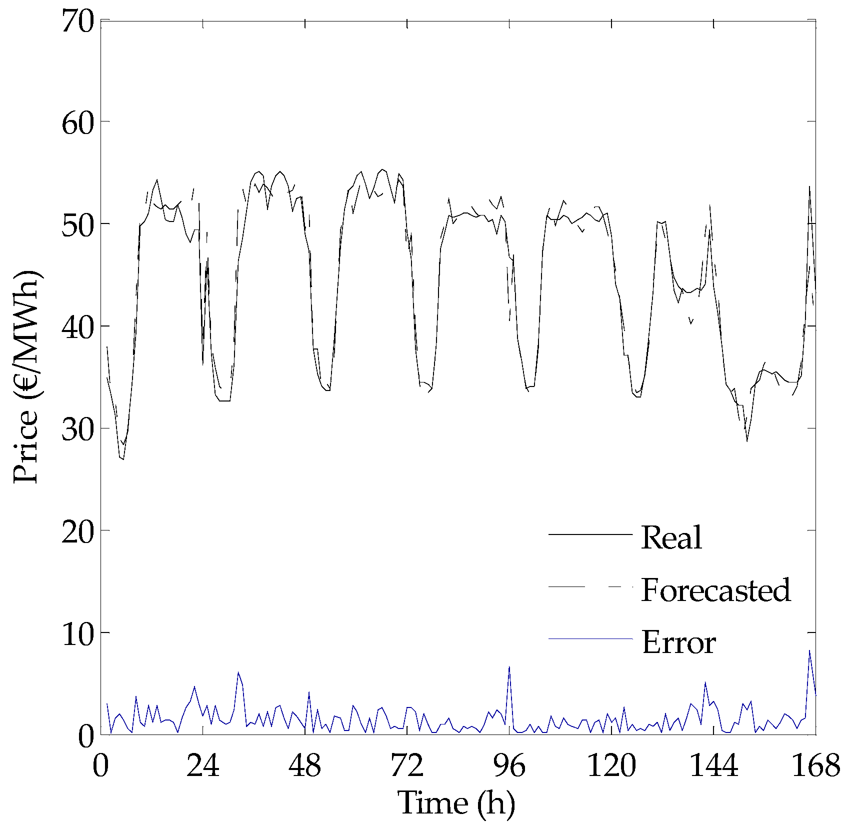
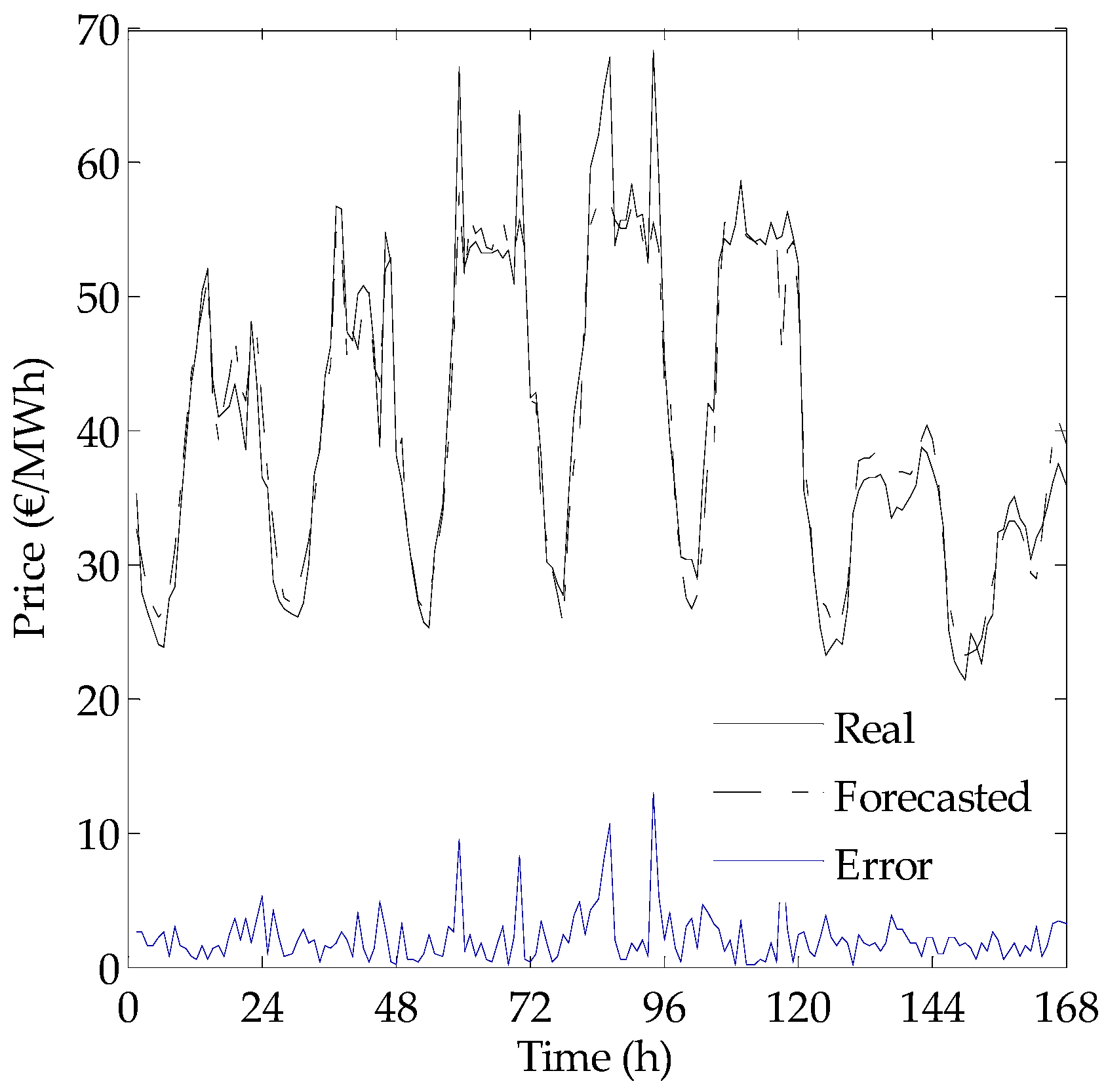
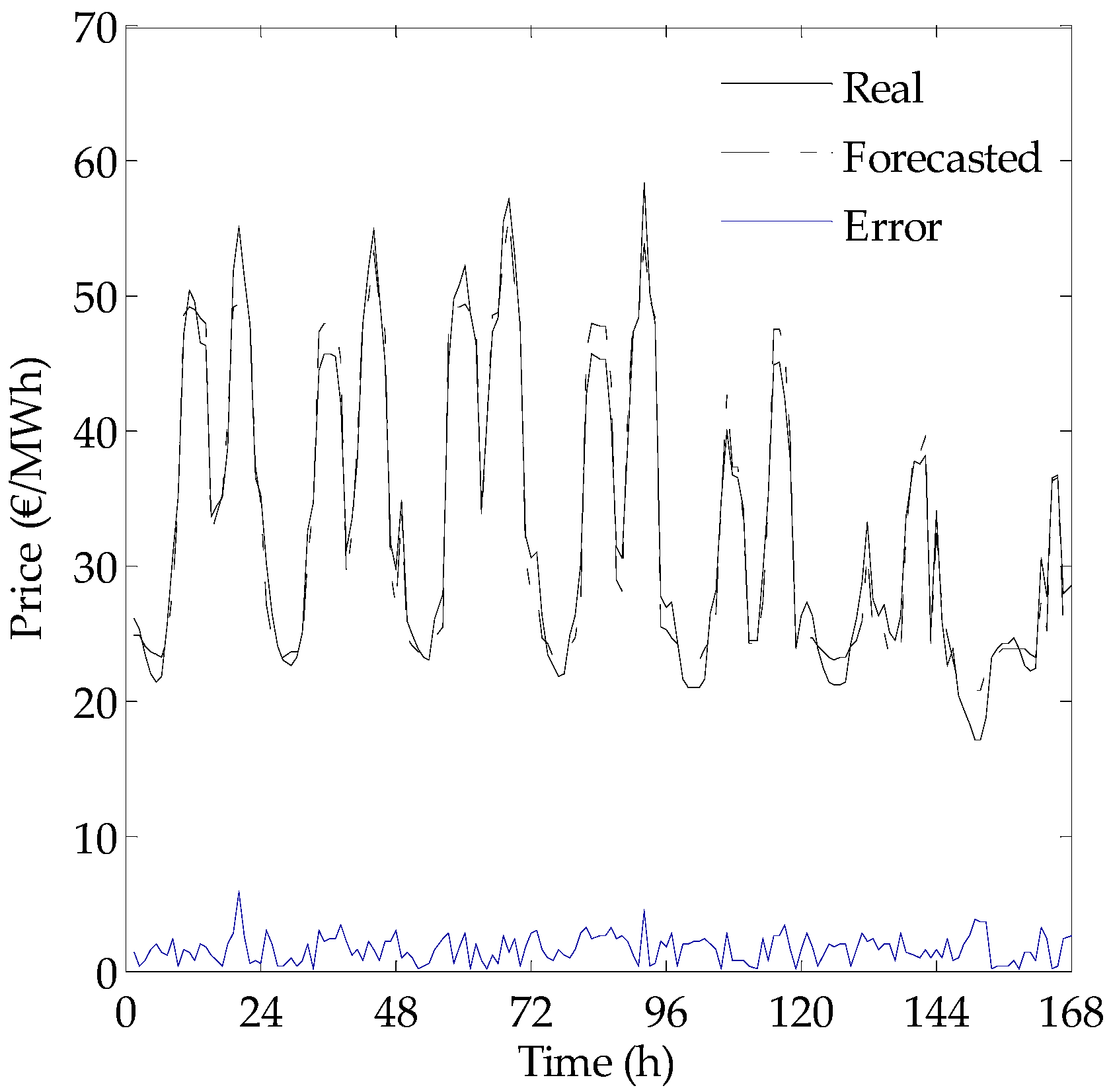
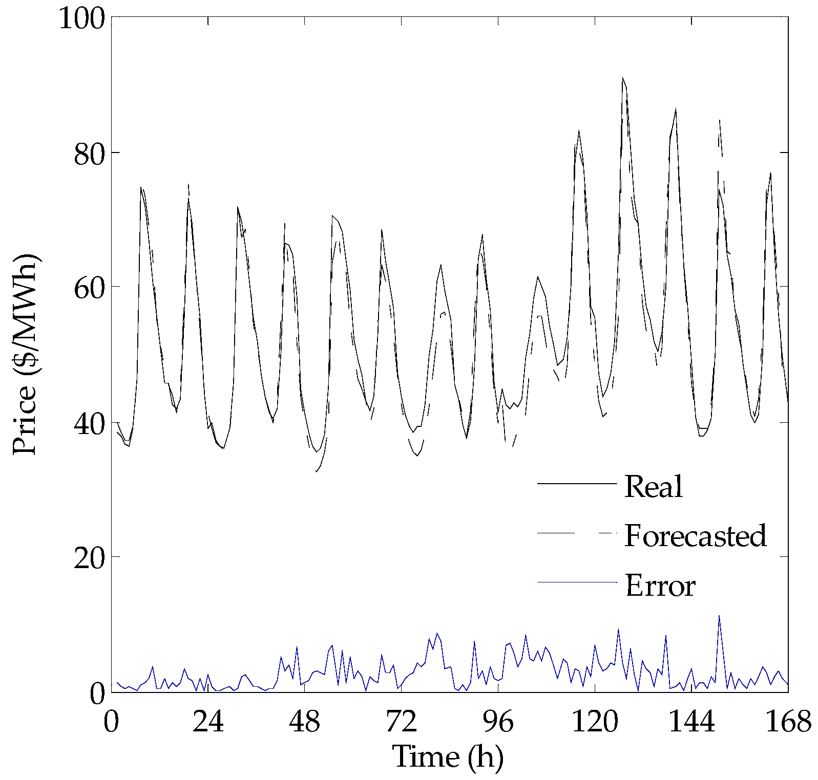
3.1. Electricity Market Prices Forecasting

As briefly stated before, the HWDA approach is used first to forecast EMP for the next 168 and 24 h considering the historical data from the Spanish market available in [54].

As mentioned in [10,21], this market has features that are difficult to forecast due to influences from dominant players, which are reflected in historical data. The EMP historical data used for the Spanish market date back to the year 2002, allowing a clear and fair comparison with the already published results from other proposed methodologies, considering the same four test weeks of the year 2002, which are consistent with the four seasons. As stated before, only EMP historical data sets were used, for the reasons stated above, otherwise a correct comparative study would not be possible.

The HWDA approach forecasts the next 168 h of EMP considering the previous 1008 h (six weeks), which are used as input sets. In order to avoid over-training during the learning process, very large training sets are not used. The output of the HWDA approach results in a set of 168 points representing the forecasting horizon. For day-ahead forecasting, the same idea may be followed; that is, the HWDA approach has as its input the previous six days, considering the historical data from the same market for the year 2006, which were analysed by the case studies reported in [44].

Furthermore, the HWDA approach is tested for the PJM market, forecasting the EMP for the next 24 and 168 h ahead. The historical data of electricity prices are available in [55]. Similarly to the Spanish market, no exogenous data were considered for the same reason as described above.

3.1.1. Spanish Market Results

The results obtained with the HWDA approach are provided in Figure 5, Figure 6, Figure 7 and Figure 8 for the four test weeks (168 h ahead) of 2002, where the solid and dash-dot black lines represent the actual and forecasted EMP, respectively, while the blue line at the bottom of each figure represents the resulting errors as absolute values.

Table 2. MAPE (the mean absolute percentage error) comparison considering the year 2002 Spanish market case study for 168 h ahead.

Methods	Winter	Spring	Summer	Fall	Average	Enhancement
NN [13], 2007	5.23	5.36	11.40	13.65	8.91	54.66%
FNN [11], 2006	4.62	5.30	9.84	10.32	7.52	46.28%
HIS [12], 2009	6.06	7.07	7.47	7.30	6.97	42.04%
AWNN [14], 2008	3.43	4.67	9.64	9.29	6.75	40.15%
CNEA [15], 2009	4.88	4.65	5.79	5.96	5.32	24.06%
CNN [16], 2009	4.21	4.76	6.01	5.88	5.22	22.61%
HNES [17], 2010	4.28	4.39	6.53	5.37	5.14	21.40%
MI+CNN [22], 2012	4.51	4.28	6.47	5.27	5.13	21.25%
WPA [19], 2011	3.37	3.91	6.50	6.51	5.07	20.32%
HEA [44], 2014	3.04	3.33	5.38	4.97	4.18	3.35%
HWDA	3.00	3.16	5.23	4.76	4.04	-

and

Table 3. Weekly error variance comparison considering the year 2002 Spanish market case study for 168 h ahead.

Methods	Winter	Spring	Summer	Fall	Average	Enhancement
NN [13], 2007	0.0017	0.0018	0.0109	0.0136	0.0070	82.86%
FNN [11], 2006	0.0018	0.0019	0.0092	0.0088	0.0054	77.78%
AWNN [14], 2008	0.0012	0.0031	0.0074	0.0075	0.0048	75.00%
HIS [12], 2009	0.0034	0.0049	0.0029	0.0031	0.0036	66.67%
CNEA [15], 2009	0.0036	0.0027	0.0043	0.0039	0.0036	66.67%
CNN [16], 2009	0.0014	0.0033	0.0045	0.0048	0.0035	65.71%
WPA [19], 2011	0.0008	0.0013	0.0056	0.0033	0.0027	55.56%
MI+CNN [22], 2012	0.0014	0.0014	0.0033	0.0022	0.0021	42.86%
HNES [17], 2010	0.0013	0.0015	0.0033	0.0022	0.0021	42.86%
HEA [44], 2014	0.0008	0.0011	0.0026	0.0014	0.0015	20.00%
HWDA	0.0007	0.0008	0.0022	0.0010	0.0012	-

shows the comparative MAPE criterion and weekly error variance criterion results, respectively, between the HWDA approach and ten previous published methodologies, namely NN [13], FNN [11], AWNN [14], HIS [12], CNEA [15], CNN [16], WPA [19], mutual information with composite NN (MI+CNN) [22], and hybrid evolutionary algorithm (HEA) [44], indicating the enhancements as the percentage evolution between the HWDA approach and the respective comparative methodology under analysis.

When the HWDA approach was used, the MAPE criterion reached an average value of 4.04%, which is significant, even when it is compared for each week independently or considering the improvements over all comparative methodologies. The weekly error variance criterion results obtained using the HWDA approach reached an average value of 0.0012, showing a notable accuracy compared with the other methodologies described and reported, even when its improvements are analysed independently.

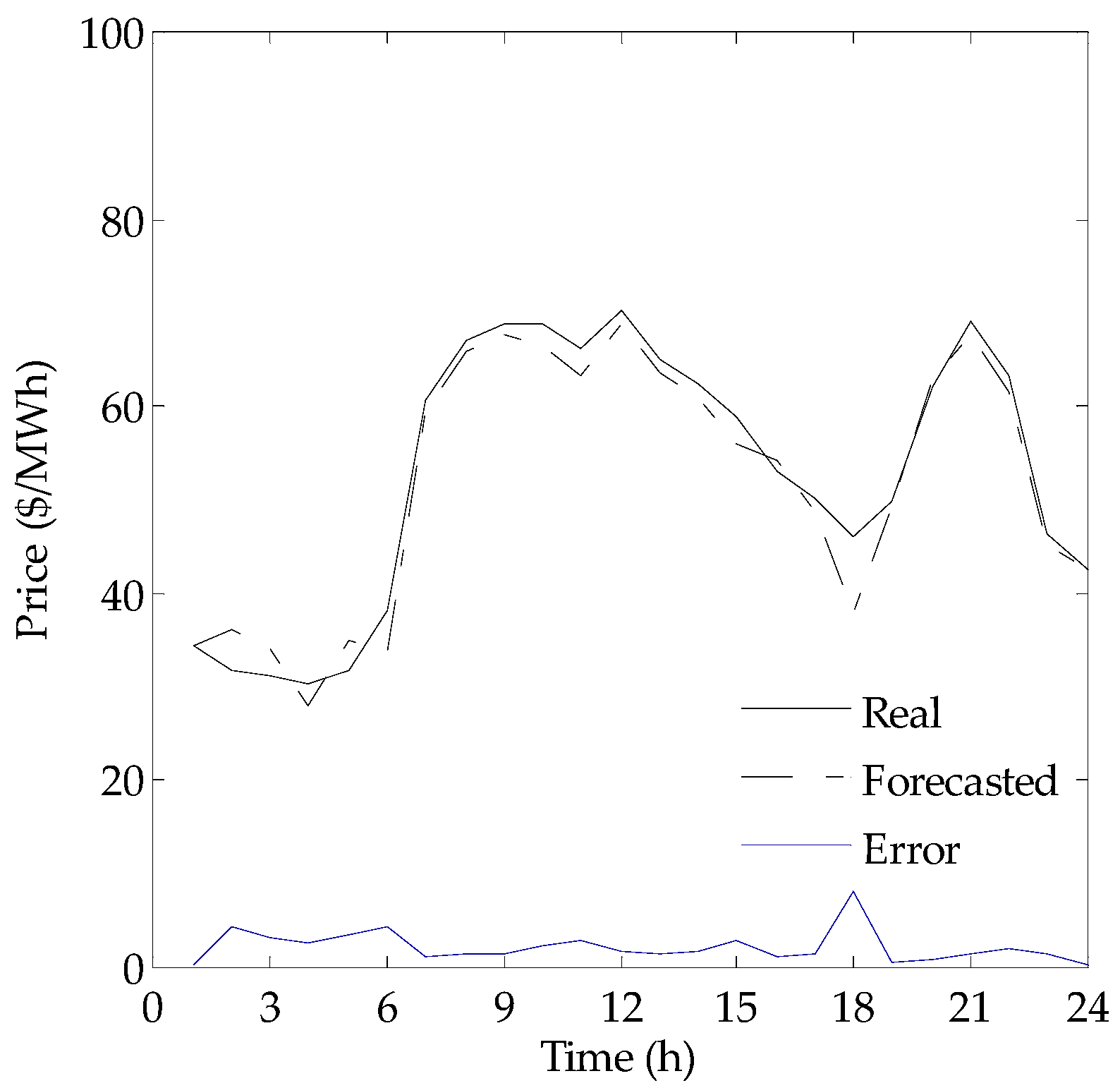
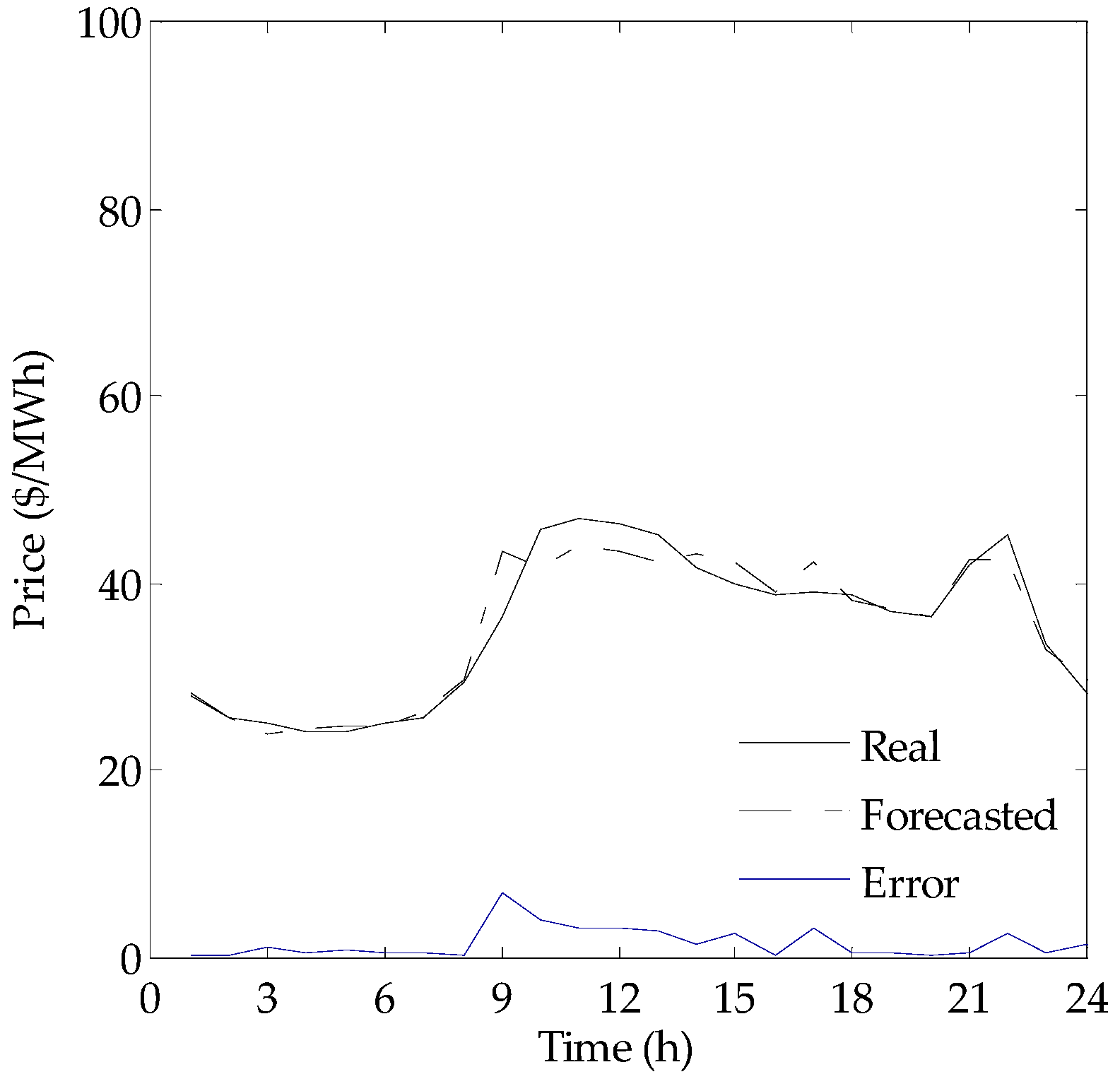
3.1.2. PJM (Pennsylvania-New Jersey-Mary) Land Market Results

The HWDA approach was also used to forecast the EMP considering the historical data from the PJM market, available in [55], providing results for the next 24 and 168 h ahead. As in the previous case study, no exogenous data are taken into account. Figure 9, Figure 10 and Figure 11 illustrate some results for some days and weeks tested considering the historical data of 2006 for the PJM market, and the same condition as described in [44] is applied to give a clear and fair comparison with other published methodologies. Moreover, in all figures, the solid and dash-dot black lines represent the actual and forecasted EMP, respectively, while the blue line at the bottom of each figure represents the resulting errors as absolute values.

Table 4. MAPE (the mean absolute percentage error) comparison considering the year 2006 PJM (Pennsylvania-New Jersey-Mary) land market case study for 24/168 h ahead.

	HNES [17], 2010	Hybrid [44], 2010	CNEA [15], 2009	HEA [44], 2014	HWDA
Jan. 20	4.98	3.71	4.73	3.29	3.22
Feb. 10	4.10	2.85	4.50	2.80	2.71
Mar. 5	4.45	5.48	4.92	3.32	3.27
Apr. 7	4.67	4.17	4.22	3.55	3.42
May 13	4.05	4.06	3.96	3.43	3.40
Feb. 1–7	4.62	5.27	4.02	3.11	3.09
Feb. 22–28	4.66	5.01	4.13	3.08	3.02
Average	4.50	4.36	4.35	3.23	3.16
Enhancement	29.78%	27.52%	27.36%	2.17%	-

and

Table 5. Error variance comparison considering the year 2006 PJM (Pennsylvania-New Jersey-Mary) land market case study for 24/168 h ahead.

	CNEA [15], 2009	Hybrid [44], 2010	HNES [17], 2010	HEA [44], 2013	HWDA
Jan. 20	0.0031	0.0010	0.0020	0.0010	0.0010
Feb. 10	0.0036	0.0015	0.0012	0.0009	0.0008
Mar. 5	0.0042	0.0033	0.0015	0.0011	0.0010
Apr. 7	0.0022	0.0013	0.0018	0.0011	0.0011
May 13	0.0027	0.0015	0.0013	0.0012	0.0012
Feb. 1–7	0.0044	0.0037	0.0016	0.0012	0.0011
Feb. 22–28	0.0035	0.0025	0.0017	0.0017	0.0016
Average	0.0034	0.0021	0.0016	0.0012	0.0011
Enhancement	67.65%	47.62%	45.45%	8.33%	-

shows the MAPE and error variance results, respectively, for the HWDA approach and four other methodologies. When using the HWDA approach, the MAPE criterion reached an average value of 3.16% and the error variance reached an average of 0.0011, which is notable for this competitive market.

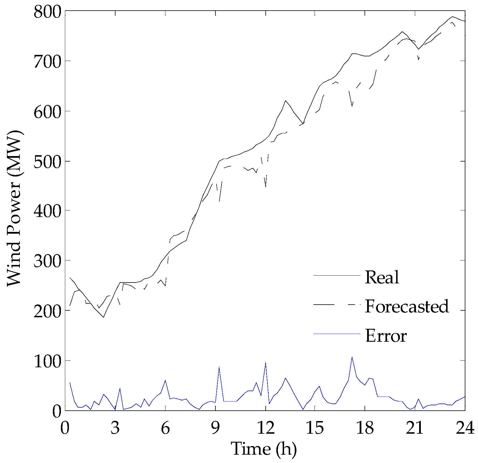
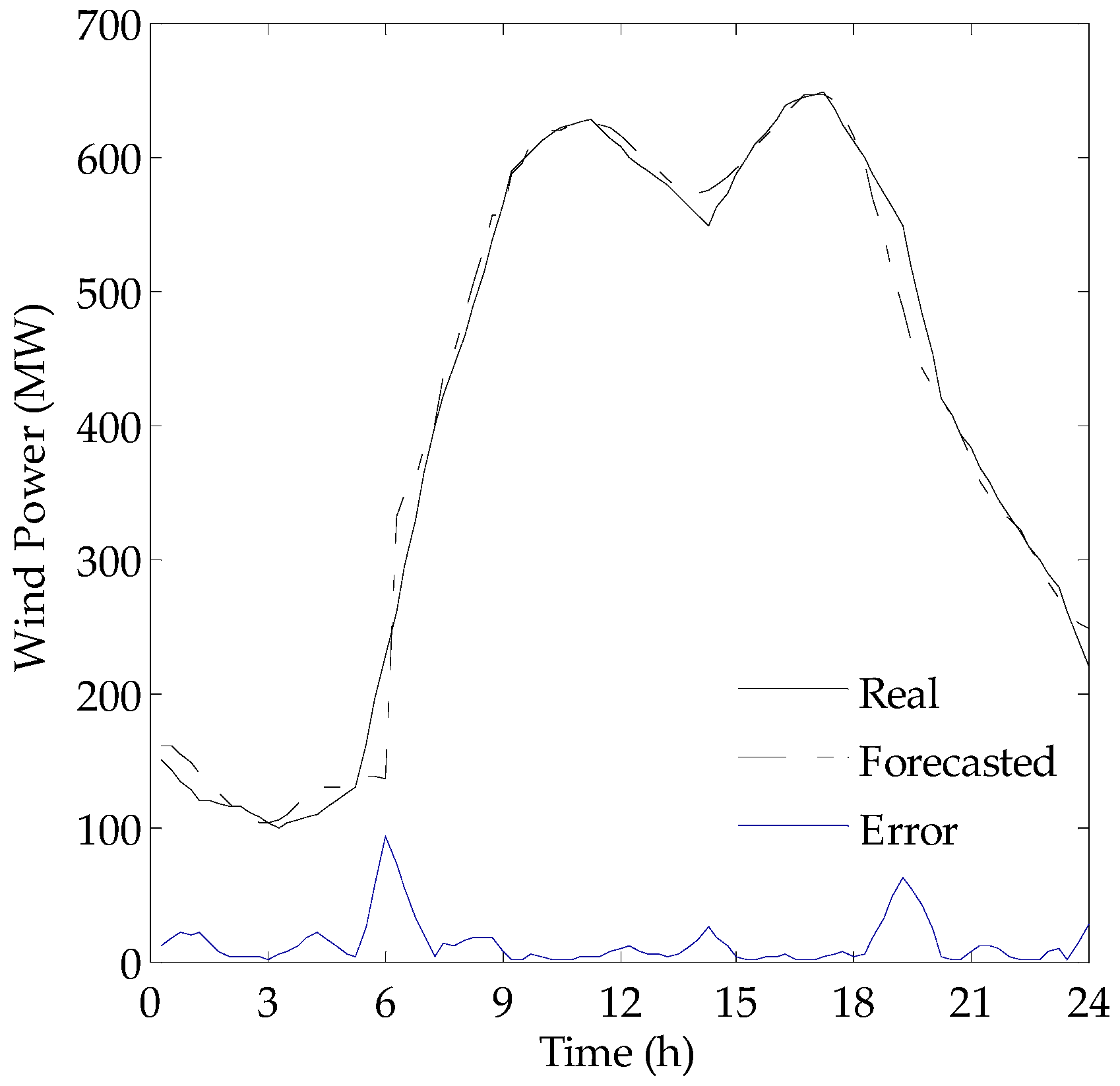
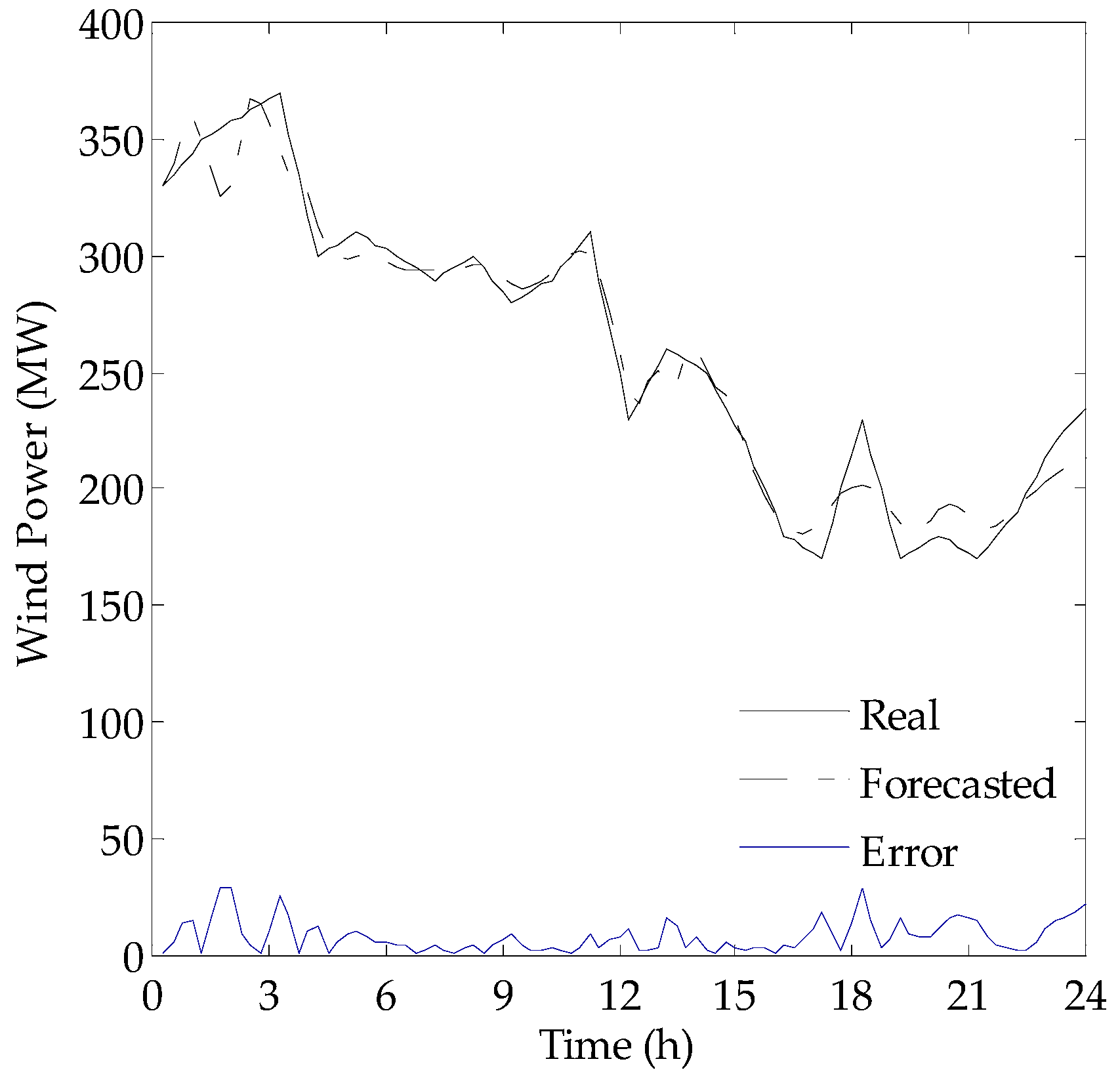
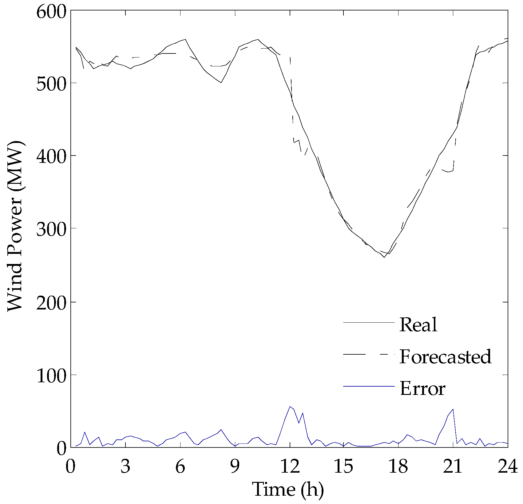
3.2. Wind Power Forecasting

The HWDA approach was used to forecast the wind power for 3 h ahead with a time-step of 15 min until the forecast for the whole 24 h ahead was complete, considering the historical data of wind power in Portugal between 2007 and 2008 as described in [45,53] and considering the different seasons of the year. Also, as in the previous case studies, to allow a fair and clean comparison, only historical wind power data are considered, for the same reason as described above. Figure 12, Figure 13, Figure 14 and Figure 15 show the numerical wind power results for winter, spring, summer, and autumn days, respectively, where solid and dash-dot black lines represent the actual and forecasted wind power, respectively, while the blue line in the bottom figures represents the errors as absolute values. For all results, it is possible to observe how the HWDA approach correctly forecasts the unexpected and abrupt changes of the wind power profile, that is, its uncertainty behaviour during the whole day of forecasting.

Table 6. MAPE (the mean absolute percentage error) comparison for wind power forecasting.

	Winter	Spring	Summer	Fall	Average	Enhancement
NN [29]	9.51	9.92	6.34	3.26	7.26	53.58%
NF [32]	8.85	8.96	5.63	3.11	6.64	49.25%
WNF [34]	8.34	7.71	4.81	3.08	5.99	43.74%
WPA [35]	6.47	6.08	4.31	3.07	4.98	32.33%
HEA [45]	5.74	3.49	3.13	2.62	3.75	11.28%
HWDA	5.08	3.19	2.96	2.27	3.37	-

and

Table 7. Daily error variance comparison for wind power forecasting.

	Winter	Spring	Summer	Fall	Average	Enhancement
NN [29]	0.0044	0.0106	0.0043	0.0010	0.0051	76.47%
NF [32]	0.0041	0.0086	0.0038	0.0008	0.0043	72.09%
WNF [34]	0.0046	0.0051	0.0021	0.0011	0.0032	62.50%
WPA [35]	0.0021	0.0035	0.0016	0.0011	0.0021	42.86%
HEA [45]	0.0019	0.0015	0.0010	0.0008	0.0013	7.69%
HWDA	0.0017	0.0016	0.0007	0.0006	0.0012	-

provide a comparative study between the HWDA approach using MAPE and the daily error variance criterion and five other previously published methodologies, namely NN [29], NF [32], WNF [34], WPA [35], and HEA [45], respectively. When the HWDA approach is used, the MAPE criterion has an average value of 3.37%, representing an enhancement of 11.28% compared to the HEA methodology, which is again significant.

Furthermore, the daily error variance obtained using the HWDA approach has an average value of 0.0013%, presenting lower uncertainty in the forecasts done, and again, in all results the HWDA approach shows better accuracy in comparison with analyses of the same real case by all other previously published methodologies.

Finally,

Table 8. NMAE (the normalized root mean square error) comparison for wind power forecasting.

	Winter	Spring	Summer	Fall	Average	Enhancement
NN [29]	5.22	3.72	2.35	2.15	3.36	84.23%
NF [32]	4.86	3.36	2.09	2.05	3.09	82.85%
WNF [34]	4.58	2.89	1.78	2.03	2.82	81.21%
WPA [35]	3.56	2.28	1.60	2.02	2.37	77.64%
HEA [45]	2.73	1.48	0.74	1.10	1.51	64.90%
HWDA	0.94	0.49	0.28	0.39	0.53	-

and

Table 9. NRMSE (the normalized root mean square error) comparison for wind power forecasting.

	Winter	Spring	Summer	Fall	Average	Enhancement
HEA [45]	3.60	3.18	1.78	2.07	2.66	39.47%
HWDA	2.19	1.27	1.81	1.18	1.61	-

show a comparison of the results obtained with the HWDA approach according to the NMAE and NRMSE criteria, respectively. In all cases analysed, it is possible to observe that the HWDA approach gave better results than the other published methodologies considering the same cases studies. The proposed HWDA approach was performed on a standard PC equipped with an Intel Core i7-3537U, 2 GHz CPU and 4 GB of RAM with Windows 10 and the MATLAB^®2016a platform. The authors used the ANFIS and WT structure functions available in MATLAB toolboxes, while DEEPSO was programmed from scratch in MATLAB considering the information available in [49,50,51,52].

4. Conclusions

An enhanced HWDA approach was proposed in this paper for short-term EMP and wind power forecasting considering real cases studies, specifically the analyses from Spanish and PJM markets, as well as the wind power behavior in Portugal. The innovative and successful combination of WT, DEEPSO and ANFIS provided interesting and valuable results. The main findings resulting from this study are related to the lower forecasting errors attained while providing an acceptable computational time. The MAPE criterion reached an average value of 4.04% for the Spanish Market, surpassing all other methodologies, and for the PJM market reached an average value of 3.16%. Regarding the wind power forecasting results, the MAPE criterion had an average value of 3.37%. Lower error variances were also obtained in all cases. Moreover, the computational time required for HWDA approach was less than two min, on average, for the EMP results, and for wind power forecasting took less than one min per iteration. Hence, the overall results obtained with the HWDA approach provided an excellent trade-off between computational time and accuracy, which is crucial for real-life and real-time applications.

References

1. Dufo-López, R.; Bernal-Agustín, J.L.; Monteiro, C. New methodology for the optimization of the management of wind farms, including energy storage. Appl. Mech. Mater. 2013, 330, 183–187. [Google Scholar] [CrossRef]
2. Catalão, J.P.S. Smart and Sustainable Power Systems: Operations, Planning, and Economics of Insular Electricity Grids, 1st ed.; CRC Press, Taylor and Francis Group: Boca Raton, FL, USA, 2015. [Google Scholar]
3. Rodrigues, E.M.G.; Osório, G.J.; Godina, R.; Bizuayehu, A.W.; Lujano-Rojas, J.M.; Matias, J.C.O.; Catalão, J.P.S. Modelling and sizing of NaS (sodium sulfur) battery energy storage system for extending wind power performance in Crete Island. Energy 2015, 90, 1606–1617. [Google Scholar] [CrossRef]
4. Li, L.; Wang, J. Sustainable energy development scenario forecasting and energy saving policy analysis of China. Renew. Sust. Energy Rev. 2016, 58, 718–724. [Google Scholar]
5. Weron, R. Electricity price forecasting: A review of the state-of-the-art with a look into the future. Int. J. Forecas. 2014, 30, 1030–1081. [Google Scholar] [CrossRef]
6. Chang, W.Y. A literature review of wind forecasting methods. J. Power Energy Eng. 2014, 2, 161–168. [Google Scholar] [CrossRef]
7. Ren, Y.; Suganthan, P.N.; Srikanth, N. Ensemble methods for wind and solar power forecasting—A state of the art review. Renew. Sust. Energy Rev. 2015, 50, 82–91. [Google Scholar] [CrossRef]
8. Okumus, I.; Dinler, A. Current status of wind energy forecasting and a hybrid method for hourly predictions. Energy Conv. Manag. 2016, 123, 362–371. [Google Scholar] [CrossRef]
9. Wang, X.; Guo, P.; Huang, X. A review of wind power forecasting models. Energy Proc. 2011, 12, 770–778. [Google Scholar] [CrossRef]
10. Conejo, A.J.; Plazas, M.A.; Espínola, R.; Molina, A.B. Day-ahead electricity price forecasting using wavelet transform and ARIMA models. IEEE Trans. Power Syst. 2005, 20, 1035–1042. [Google Scholar] [CrossRef]
11. Amjady, N. Day-ahead price forecasting of electricity markets by a new fuzzy neural network. IEEE Trans. Power Syst. 2006, 21, 887–896. [Google Scholar] [CrossRef]
12. Amjady, N.; Hemmati, H. Day-ahead price forecasting of electricity markets by a hybrid intelligent system. Euro Trans. Electron. Power 2006, 19, 89–102. [Google Scholar] [CrossRef]
13. Catalão, J.P.S.; Mariano, S.J.P.S.; Mendes, V.M.F.; Ferreira, L.A.F.M. Short-term electricity prices forecasting in a competitive market: A neural network approach. Electron Power Syst. Res. 2007, 77, 1297–1304. [Google Scholar] [CrossRef]
14. Pindoriya, N.M.; Singh, S.N.; Singh, S.K. An adaptive wavelet neural network-based energy price forecasting, in electricity market. IEEE Trans. Power Syst. 2008, 23, 1423–1432. [Google Scholar] [CrossRef]
15. Amjady, N.; Keynia, F. Day-ahead price forecasting of electricity markets by mutual information technique and cascaded neuro-evolutionary algorithm. IEEE Trans. Power Syst. 2009, 24, 306–318. [Google Scholar] [CrossRef]
16. Amjady, N.; Daraeepour, A. Design of input vector for day-ahead price forecasting of electricity markets. Exp. Syst. Appl. 2009, 36, 12281–12294. [Google Scholar] [CrossRef]
17. Amjady, N.; Keynia, F. Application of a new hybrid neuro-evolutionary system for day-ahead price forecasting of electricity markets. Appl. Soft Comput. 2010, 10, 784–792. [Google Scholar] [CrossRef]
18. Wu, L.; Shahidehpour, M. A hybrid model for day-ahead price forecasting. IEEE Trans. Power Syst. 2010, 25, 1519–1530. [Google Scholar]
19. Catalão, J.P.S.; Pousinho, H.M.I.; Mendes, V.M.F. Hybrid wavelet-PSO-ANFIS approach for short-term electricity prices forecasting. IEEE Trans. Power Syst. 2011, 26, 137–144. [Google Scholar] [CrossRef]
20. Shafie-khah, M.; Moghaddam, M.P.; Sheikh-El-Eslami, M.K. Price forecasting of day-ahead electricity markets using a hybrid forecast method. Energy Convers. Manag. 2011, 52, 2165–2169. [Google Scholar] [CrossRef]
21. González, V.; Contreras, J.; Bunn, D.W. Forecasting power prices using a hybrid fundamental-econometric model. IEEE Trans. Power Syst. 2012, 27, 363–372. [Google Scholar] [CrossRef]
22. Keynia, F. A new feature selection algorithm and composite neural network for electricity price forecasting. Eng. Appl. Artif. Intell. 2012, 25, 1687–1697. [Google Scholar] [CrossRef]
23. Shayeghi, H.; Ghasemi, A. Day-ahead electricity prices forecasting by a modified CGSA technique and hybrid WT in LSSVM based scheme. Energy Convers. Manag. 2013, 74, 482–491. [Google Scholar] [CrossRef]
24. Miranian, A.; Abdollahzade, M.; Hassani, H. Day-ahead electricity price analysis and forecasting by singular spectrum analysis. IET Gener. Trans. Distrib. 2013, 7, 337–346. [Google Scholar] [CrossRef]
25. Elattar, E.; Shebin, E.K. Day-ahead price forecasting of electricity markets based on local informative vector machine. IET Gener. Transm. Distrib. 2013, 7, 1063–1071. [Google Scholar] [CrossRef]
26. Kim, M.K. Short-term price forecasting of Nordic power market by combination Levenberg-Marquardt and cuckoo search algorithms. IET Gen. Trans. Distrib. 2015, 9, 1553–1563. [Google Scholar] [CrossRef]
27. Alamaniotis, M.; Bargiotas, D.; Bourbakis, N.G.; Tsoulalas, L.H. Genetic optimal regression of relevance vector machines for electricity pricing signal forecasting in smart grids. IEEE Trans. Smart Grid 2015, 6, 2997–3005. [Google Scholar] [CrossRef]
28. Jursa, R.; Rohrig, K. Short-term wind power forecasting using evolutionary algorithms for the automated specification of artificial intelligence models. Int. J. Forecast. 2008, 24, 694–709. [Google Scholar] [CrossRef]
29. Catalao, J.P.S.; Pousinho, H.M.I.; Mendes, V.M.F. An artificial neural network approach for short-term wind power forecasting in Portugal. Eng. Intell. Syst. Electron. Eng. Commun. 2009, 17, 5–11. [Google Scholar]
30. Rosado, I.J.R.; Jimenez, L.A.F.; Monteiro, C.; Sousa, J.; Bessa, R. Comparison of two new short-term wind-power forecasting systems. Renew. Energy 2009, 34, 1848–1854. [Google Scholar] [CrossRef]
31. Amjady, N.; Keynia, F.; Zareipour, H. Short-term wind power forecasting using ridgelet neural network. Electr. Power Syst. Res. 2011, 81, 2099–2107. [Google Scholar] [CrossRef]
32. Catalão, J.P.S.; Pousinho, H.M.I.; Mendes, V.M.F. Hybrid intelligent approach for short-term wind power forecasting in Portugal. IET Renew. Power Gener. 2011, 5, 251–257. [Google Scholar] [CrossRef]
33. Catalão, J.P.S.; Pousinho, H.M.I.; Mendes, V.M.F. Short-term wind power forecasting in Portugal by neural network and wavelet transform. Renew. Energy 2011, 36, 1245–1251. [Google Scholar] [CrossRef]
34. Pousinho, H.M.I.; Mendes, V.M.F.; Catalão, J.P.S. Application of adaptive neuro-fuzzy inference for wind power short-term forecasting. IEEJ Trans. Electr. Electron. Eng. 2011, 6, 571–576. [Google Scholar] [CrossRef]
35. Catalão, J.P.S.; Pousinho, H.M.I.; Mendes, V.M.F. Hybrid wavelet-PSO-ANFIS approach for short-term wind power forecasting in Portugal. IEEE Trans. Sustain. Energy 2011, 2, 50–59. [Google Scholar]
36. Liu, Y.; Shi, J.; Yang, Y.; Lee, W.J. Short-term wind-power prediction based on wavelet transform-support vector machine and statistic-characteristics analysis. IEEE Trans. Ind. Appl. 2012, 48, 1136–1141. [Google Scholar] [CrossRef]
37. Bhaskar, K.; Singh, S. AWNN-assisted wind power forecasting using feedforward neural network. IEEE Trans. Sustain. Energy 2012, 3, 306–315. [Google Scholar] [CrossRef]
38. Haque, A.U.; Mandal, P.; Meng, J.; Srivastava, A.K.; Tseng, T.L.; Senjyu, T. A novel hybrid approach based on wavelet transform and fuzzy ARTMAP networks for predicting wind farm power production. IEEE Trans. Ind. Appl. 2013, 49, 2253–2261. [Google Scholar] [CrossRef]
39. Liu, D.; Niu, D.; Wang, H.; Fan, L. Short-term wind speed forecasting using wavelet transform and support vector machines optimized by genetic algorithm. Renew. Energy 2013, 62, 592–597. [Google Scholar] [CrossRef]
40. Skittides, C.; Früh, W.G. Wind forecasting using principal component analysis. Renew. Energy 2014, 69, 365–374. [Google Scholar] [CrossRef]
41. Mandal, P.; Zareipour, H.; Rosehart, W.D. Forecasting aggregated wind power production of multiple wind farms using hybrid wavelet-PSO-NNs. Int. J. Energy Res. 2014, 38, 1654–1666. [Google Scholar] [CrossRef]
42. Yeh, W.C.; Yeh, Y.M.; Chang, P.C.; Ke, Y.C. Forecasting wind power in the Mai Liao wind farm based on the multi-layer perceptron artificial neural network model with improved simplified swarm optimization. Elect. Power Energy Syst. 2014, 55, 741–748. [Google Scholar] [CrossRef]
43. Chitsaz, H.; Amjady, N.; Zareipour, H. Wind power forecast using wavelet neural network trained by improved clonal selection algorithm. Energy Conv. Manag. 2015, 89, 588–598. [Google Scholar] [CrossRef]
44. Osório, G.J.; Matias, J.C.O.; Catalão, J.P.S. Electricity prices forecasting by a hybrid evolutionary-adaptive methodology. Energy Conv. Mang. 2014, 80, 363–373. [Google Scholar] [CrossRef]
45. Osório, G.J.; Matias, J.C.O.; Catalão, J.P.S. Short-term wind power forecasting using adaptive neuro-fuzzy inference system combined with evolutionary particle swarm optimization, wavelet transform and mutual information. Renew. Energy 2015, 75, 301–307. [Google Scholar] [CrossRef]
46. Eynard, J.; Grieu, S.; Polit, M. Wavelet-based multi-resolution analysis and artificial neural networks, for forecasting temperature and thermal power consumption. Eng. App. Art. Intell. 2011, 24, 501–516. [Google Scholar] [CrossRef]
47. Amjady, N.; Keynia, F. Short-term loads forecasting of power systems by combining wavelet transform and neuro-evolutionary algorithm. Energy 2009, 34, 46–57. [Google Scholar] [CrossRef]
48. Miranda, V.; Carvalho, L.M.; Rosa, M.A.; Silva, A.M.L.; Singh, C. Improving power system reliability calculation efficiency with EPSO variants. IEEE Trans. Power Syst. 2009, 24, 1772–1779. [Google Scholar] [CrossRef]
49. Miranda, V.; Alves, R. Differential evolutionary particle swarm optimization (DEEPSO): A successful hybrid. In Proceedings of the 1st BRICS Congress on Computational Intelligence and 11th Brazilian Congress on Computational Intelligence (BRICS-CCI and CBIC), Recife, Brazil, 8–11 September 2013.
50. Carvalho, L.M.; Loureiro, F.; Sumaili, J.; Keko, H.; Miranda, V.; Marcelino, C.G.; Wanner, E.F. Statistical tuning of DEEPSO soft constraints in the security constrained optimal power flow problem. In Proceedings of the 2015 18th International Conference on Intelligent System Application to Power Systems (ISAP), Porto, Portugal, 11–17 September 2015.
51. Pinto, P.; Carvalho, L.M.; Sumaili, J.; Pinto, M.S.S.; Miranda, V. Coping with wind power uncertainty in unit commitment: A robust approach using the new hybrid metaheuristic DEEPSO. In Proceedings of the Towards Future Power Systems and Emerging Technologies, Powertech Eindhoven, Eindhoven, The Netherlands, 29 June–2 July 2015.