1. Introduction
It is important to understand biological behavior as a system. For this purpose, systems biology has been established as a new research field [
1,
2]. One of the practical applications in systems biology is gene therapy technologies (see, e.g., [
3]). In gene therapy, the expression of certain genes must be controlled, and such a problem can be formulated as a control problem. In other words, control of gene regulatory networks corresponds to therapeutic interventions realized by radiation, chemotherapy, and so on. Thus, control theory of gene regulatory networks is important for developing medical services in the future. Furthermore, from the viewpoint of experimental study, several results on control of gene regulatory networks have been obtained in [
4,
5,
6,
7]. For example, in [
5], it was shown that cellular behavior can be regulated by control. These results suggest that feedback control of biological systems can be implemented. Motivated by the above background, we are developing theory of control methods for gene regulatory networks.
In developing a control method of gene regulatory networks, first, it is important to consider what mathematical model is utilized. A gene regulatory network is modeled by discrete dynamical systems (e.g., Bayesian networks, Boolean networks (BNs) [
8]), continuous dynamical systems (e.g., differential/difference equations), or hybrid dynamical systems (e.g., piecewise affine models) (see, e.g., [
9] for further details). In control theory, BNs and piecewise affine models are frequently utilized (see, e.g., [
10] for control of a biological system modeled by a piecewise affine model). The control problem of hybrid systems is generally reduced to a mixed integer programming problem, in which continuous variables and binary variables are decision variables, and the computation time to solve it is frequently too long. Hence, a class of gene regulatory networks is limited to those with a small network. A BN is a mathematical model whose interactions between genes are expressed by Boolean functions [
8]. That is, gene expression is approximated by a binary value (0 or 1). Since a BN is too simple, there is a possibility that biological behavior is not precisely modeled (see, e.g., [
11]). On the other hand, this model can be relatively applied to large-scale systems. This advantage is focused on, and a BN is utilized in the first step of developing control theory of gene regulatory networks. Furthermore, a probabilistic Boolean network (PBN) [
12] and a context-sensitive PBN [
13,
14] have been proposed as the extended models of BNs. In a PBN, at each discrete time, a Boolean function is randomly chosen from the candidates of Boolean functions. In a context-sensitive PBN, the time of choosing a Boolean function is also selected randomly. Hence, a context-sensitive PBN is a generalized version of a PBN.
In the last decade, many results on control of BNs and PBNs have been obtained so far (see, e.g., [
15,
16,
17,
18,
19,
20,
21,
22,
23,
24,
25,
26,
27,
28,
29,
30,
31,
32]). Especially, analysis and control methods using the semi-tensor product (STP) method have been widely studied (see, e.g., [
33,
34,
35,
36,
37,
38,
39,
40,
41,
42,
43]). In the review paper [
44], many methods for PBNs, e.g., construction and inference methods, structural intervention methods, and control methods, have been explained in a comprehensive manner. Of course, it is difficult to understand details of individual methods by reading only [
44]. It is also significant to restrict topics and explain details. In this review paper, our previously proposed methods [
23,
24] in optimal external control of PBNs, i.e., a polynomial optimization approach and an integer programming approach are explained. Comparing our methods with other existing methods, the main advantage of our methods is that a relatively large-scale PBN can be handled. In many existing control methods (e.g., [
19,
20,
21,
30,
32,
36]), transition probability matrices with
must be manipulated (
n is the number of genes). As a result, a class of PBNs is restricted (see also
Section 5 for further details). In our methods, transition probability matrices are not used. Moreover, since several solvers are available, optimization-based approaches are useful. To the best of our knowledge, such approaches have not been studied sufficiently, and their development in the future is necessary.
First, we introduce an optimal control method using polynomial optimization. In this method, the expected value of the state in PBN is modeled by a polynomial system, which can be directly obtained by Boolean functions and information on probabilities. Then, the finite-time optimal control problem is reduced to a polynomial optimization problem. Using e.g., SparsePOP [
45], which is available on MATLAB R2006b or later, the polynomial optimization problem can be easily described and can be solved. However, there is a weakness that the polynomial optimization problem for large-scale PBNs cannot be solved owing to memory (but, comparing this method with other methods, a relatively large-scale PBN can be handled). In addition, the computational complexity of the finite-time optimal control problem of a PBN is
-hard [
17], which is harder than NP-hard (Non-deterministic Polynomial time hard). Next, we introduce an optimal control method using integer programming. Instead of the expected value of the cost function, we focus on upper and lower bounds of the cost function under a certain constraint on probabilities. Then, the optimal control problem is reduced to an integer linear programming problem.
This review paper is organized as follows. In
Section 2, PBNs are briefly explained. In
Section 3, a control method using polynomial optimization is explained. In
Section 4, a control method using integer programming is explained. In
Section 5, discussion on numerical experiments is done. In
Section 7, we conclude this review paper.
Notation: Let denote the set of real numbers. Let denote the set of n-dimensional vectors, which consists of elements 0 and 1. For a matrix/vector X, let denote the transpose of X. Let I and 0 denote the identity matrix with an appropriate size and the zero matrix/vector/scalar, respectively. For an event A, let denote the probability that A occurs. For two events , let denote the conditional probability of A given B. For two events , let denote the conditional expected value of A given B.
2. Probabilistic Boolean Networks
In this section, we introduce a probabilistic Boolean network (PBN).
Consider the following PBN:
where
is the state (e.g., the expression of genes), and
is the control input (e.g., the expression of genes), i.e., the value of
u can be arbitrarily determined,
is the discrete time. The function
is a given Boolean function consisting of logical operators such as AND (∧), OR (∨), XOR (⊕), and NOT (¬). In deterministic Boolean networks,
is uniquely determined for given
and
. In PBNs, the candidates of
are given, and for each
, selecting one Boolean function is probabilistically independent at each time. The candidates of
are denoted by
,
, and the probability that
is selected is denoted by
Then, the relation
must be satisfied.
First, we present a biological example of (deterministic) Boolean networks (BNs).
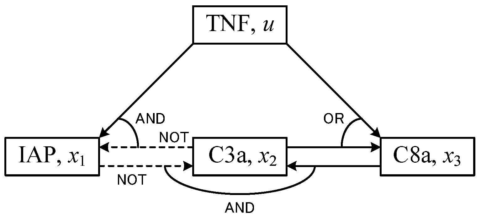
Example 1. Consider the following BN of an apoptosis network (see also Figure 1):where is the concentration level (high or low) of the inhibitor of apoptosis proteins (IAP), is the concentration level of the active caspase 3 (C3a), and is the concentration level of the active caspase 8 (C8a). The control input u corresponds to the concentration level of the tumor necrosis factor (TNF, a stimulus). This model is introduced in [46], and is a simplified version of an apoptosis network model in [47]. In this model, implies cell survival, and imply cell death. Next, we present a simple example of PBNs.
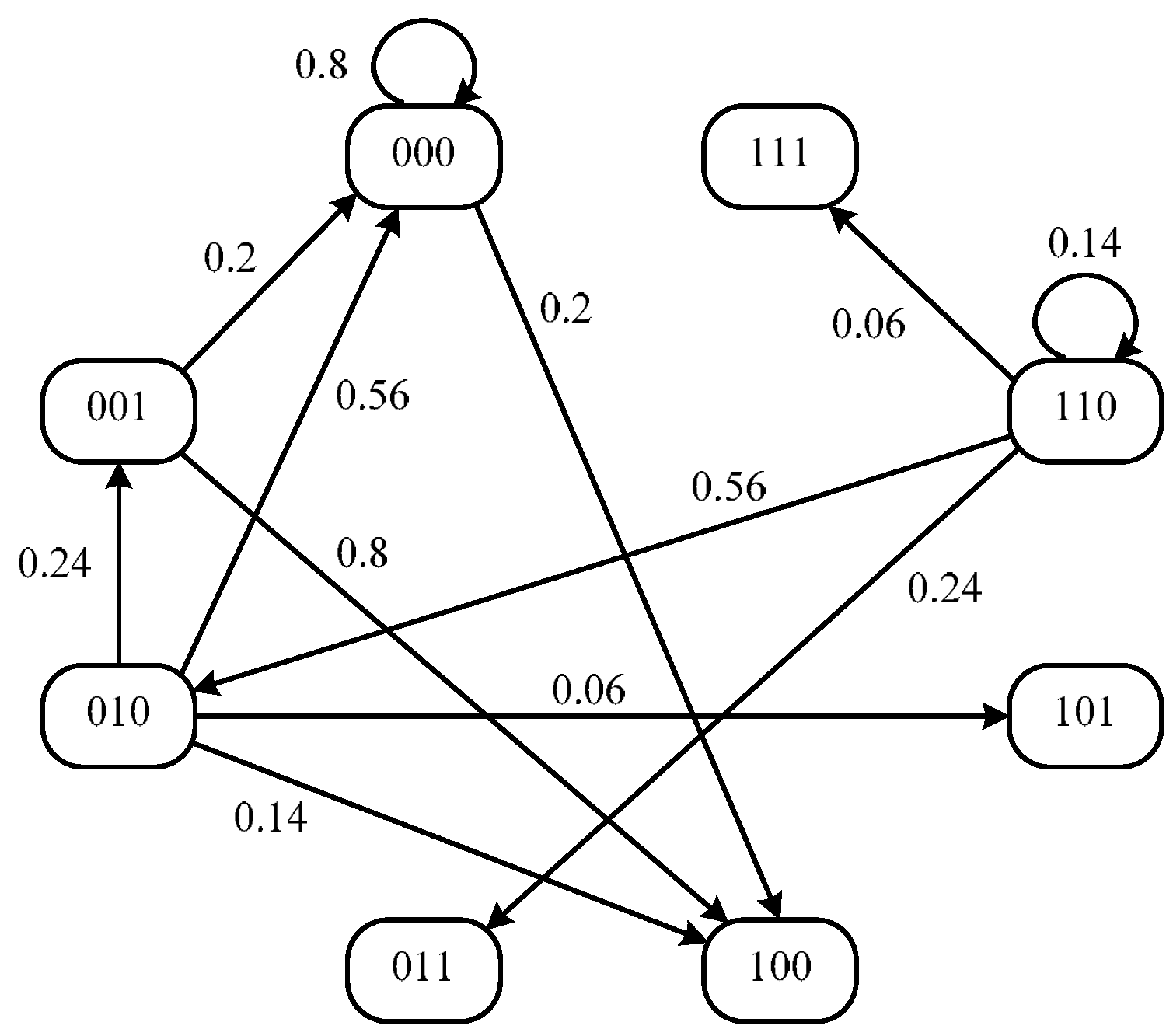
Example 2. Consider the PBN with three states and single control input. Boolean functions and probabilities are given bywhere , and hold, and we see that the relation (2) is satisfied. Next, consider the state trajectories. Then, for and , we can obtain In this example, the cardinality of the finite state set is given by , and we can obtain the state transition diagram of Figure 2 by computing the transition from each state under . In Figure 2, the number assigned to each node denotes , , (elements of the state), and the number assigned to each arc denotes the transition probability from some state to other state. Note here that, for simplicity, the state transitions from only are illustrated in Figure 2. 3. Polynomial Optimization Approach
In this section, a polynomial optimization approach to optimal control of PBNs is reviewed. The advantage of this approach is that implementation is easy by using e.g., MATLAB.
3.1. Problem Formulation
For PBN (
1), consider the following finite-time optimal control problem.
Problem 1. Suppose that, for PBN (1), the initial state and the control time N are given. Then, find a control input sequence minimizing the following cost function:where , are weighting vectors whose element is a non-negative real number. In this problem, we use some linear function with respect to the state and the control input as a cost function. Noting that the relation
holds for a binary variable
δ, it is unnecessary to add the quadratic term such as
. Moreover, one of the main purposes in control of gene regulatory networks is that the expression of a certain gene is inhibited or activated (see e.g., [
20]). Hence, simple linear cost function (
4) is sufficient.
3.2. Transformation of a PBN into a Polynomial System
Consider modeling the dynamics of the expected value of the state by a polynomial system. First, the relation between a Boolean function and a polynomial is explained as a preparation. Next, the result for a general PBN is explained. Finally, a simple example is shown.
As a preparation, the following lemma [
48] is introduced.
Lemma 1. Consider two binary variables and . Then, the following relations hold:- (i)
is equivalent to ,
- (ii)
is equivalent to ,
- (iii)
is equivalent to ,
- (iv)
is equivalent to .
By Lemma 1, a given Boolean function can be transformed into a polynomial on the real number field. For example, is equivalently transformed into .
Next, a recursive representation of a general PBN is explained. Let denote the polynomial that can be obtained from the Boolean function . Let denote the polynomial that can be obtained from the Boolean function . Hereafter, for simplicity of notation, the condition in is omitted.
In [
24], the following theorem was obtained.
Theorem 1. Suppose that, for the PBN (1), the initial state is given. Then, the expected value of the state, , is expressed as the following polynomial system: The outline of the proof is explained as follows. Since a Boolean function is independently switched for each state,
,
holds. In addition, there exists no second-order term of
in
. Then, noting that
holds, we can obtain the system (
5).
Noting that
is a polynomial, the right-hand side of the system (
5) is also a polynomial. Therefore, from Theorem 1, we see that time evolution of the expected value of the state is modeled by a polynomial system.
We present a simple example.
Example 3. Consider the PBN in Example 2 again. Suppose that, for this PBN, and are given by and , respectively. Then, from Figure 2, we can obtain . We can also obtain it in other way. By Lemma 1, and are transformed into and , respectively. Hence, we can obtain In a similar way, and can be obtained asrespectively. Next, suppose that is given by , and consider deriving . Then, noting that a Boolean function is independently switched for each state, we can obtain
By recursively repeating, we can obtain , .
From this example, we see that the expected value of the state can be expressed as a polynomial system using Theorem 1.
3.3. Reduction to a Polynomial Optimization Problem
Consider reducing Problem 1 to a polynomial optimization problem. Then, the following theorem was obtained in [
24].
Theorem 2. Problem 1 is equivalent to the following polynomial optimization problem: This theorem is immediately obtained from the following two properties: (i) the relation holds; (ii) the fact that is a binary variable is equivalent to the constraint . We remark here that this constraint is non-convex. From the practical viewpoint, it is desirable to relax this constraint to . Furthermore, from Theorem 1, we see that always holds. Hence, we set in the above polynomial optimization problem. Finally, may be eliminated from decision variables in the above problem, but its elimination is not easy. Hence, is included in a decision variable of the above problem.
A polynomial optimization problem can be solved by using e.g., SparsePOP [
45], which is available on MATLAB. In SparsePOP, polynomials can be directly described.
4. Integer Programming Approach
The effectiveness of the polynomial optimization approach is restricted because the computational complexity of Problem 1 is
-hard [
17], which is harder than NP-hard. In this section, an integer programming approach is explained. Instead of the expected value of the cost function, we focus on upper and lower bounds of the cost function. Then, the optimal control problem is reduced to an integer linear programming (ILP) problem. This method is a simplified version of our previously proposed method in [
23].
4.1. Problem Formulation
First, preparations are given. Suppose that for PBN (
1),
is given for fixed
and
. Then, we define
The parameter implies the probability that the Boolean functions are selected at time k. Furthermore, we define
The parameter implies the probability that certain Boolean functions are selected in the time interval .
Example 4. Consider the PBN in Example 2 again. Suppose , , and . In other words, , , are given as a Boolean function at time 0.
Then, we can obtain Furthermore, suppose that , , , , and . Then, we can obtain
Under these preparations, two problems (i.e., the optimal control problem and the performance evaluation problem) are formulated. First, the optimal control problem is formulated as follows.
Problem 2. Suppose that, for PBN (1), the initial state , ρ satisfying , the control time N, and the weighting vectors , whose element is a non-negative real number are given. Then, solve the following two problems. Problem 2-A: Find a control input sequence , , ⋯, minimizing the lower bound of the cost functionsatisfying the following constraint Problem 2-B: Apply the control input sequence obtained in Problem 2-A to the PBN. Then, find an upper bound of the cost function (6). Let
and
denote the obtained upper and lower bounds, respectively. In a similar way to Problem 1, a linear function with respect to
x and
u is considered as a cost function. Using the target value of the state (the offset vector)
,
may be replaced to
. Then, the cost function (
6) must be changed to
. Furthermore, by the inequality constraint (
7), combinations of Boolean functions selected with the low probability can be excluded.
Each element of the control input sequence obtained solving Problem 2 is in general different. In gene regulatory networks, it is difficult to implement such control input sequence. In this case, we must impose constraints for control input sequences. For example, one of the simple methods is that the control input is given by always 1 (active) or 0 (inactive). That is, Problem 2-A is modified as follows: find
minimizing the lower bound of the cost function (
6) under the constraint (
7).
We present a simple example.
Example 5. Consider the PBN with a single control input. Boolean functions and probabilities are given byrespectively, where . The initial state and the cost function are given byrespectively. For simplicity of discussion, ρ is given by , i.e., the constraint (7) is not imposed. Consider calculating the cost function explicitly. First, holds. Next, we can obtain the following relations at time 1
: Furthermore, can be derived as
Noting that is equivalent to (see Lemma 1), we can obtain
First, consider solving Problem 2. We can obtain the optimal solution of Problem 2-A as . The minimum value of the lower bound of the cost function is . The minimum value of the upper bounds can be obtained as (this is the solution of Problem 2-B). Next, consider the case of as an example of other constant input. Then, the upper and lower bound of the cost function can be obtained by 2 and 5, respectively. From this result, we see that a solution for Problem 2-A should be applied to the system.
Problem 2 for a simple PBN can be easily solved. However, solving this problem for a large-scale PBN is hard. Here, we introduce an integer programming approach for solving Problem 2.
4.2. Solution Method for Problem 2-A
In this subsection, a solution method for Problem 2-A is derived. The solution method for Problem 2-B will be explained in the last part of this subsection.
As a preparation, we explain one lemma. The product of multiple binary variables such as
can be linearized by using the following lemma [
49].
Lemma 2. Suppose that binary variables , are given, where is some index set. Then, is equivalent to the following linear inequalitieswhere is the cardinality of . From Lemmas 1 and 2, we see that any Boolean function can be equivalently transformed into a pair of linear functions and linear inequalities. See [
48,
49] for further details.
Consider transforming Problem 2-A into an ILP problem. Using Lemma 1,
in the PBN (
1) can be equivalently transformed into a certain polynomial. Let
denote the obtained polynomial. Then, consider the following system:
where
and
. For
, we impose the following constraint:
Next, using
and
, we define
where
. Then, the following lemma was obtained in [
23].
Lemma 3. Problem 2-A is equivalent to the following problem.
The outline of the proof is explained as follows. By deciding , Boolean functions at each time are uniquely determined. Then, we can obtain . That is, using the logarithm of the probability, can be expressed by a linear form with respect to . Hence, we can obtain
Thus, Problem 2-A is equivalent to Problem 2-C.
We consider further rewriting Problem 2-C. Since the system (
8) is a polynomial system, the system (
8) can be equivalently transformed into a linear system by using Lemma 2. Hence, the system (
8) can be transformed into the following system:
where
is an auxiliary variable, and the dimension
p can be determined from the number of the product of binary variables. For simplicity of notation, we define
,
. In addition, under
and
,
becomes a binary variable automatically. Hence, we set
,
.
We present a simple example.
Example 6. Consider the PBN in Example 5 again. Then, the system (8) can be derived as The equality constraint (9) can be derived as The state equation in the system (10) can be derived aswhere Using Lemma 2, these relations can be equivalently transformed into a set of linear inequalities. Then, holds. Thus, the linear inequality in the system (10) can be derived. Using the system (
10), consider rewriting Problem 2-C as an ILP problem. First, equality constraint (
9) is embedded in the inequality constraint in the system (
10). From the state equation in the system (
10), we can obtain
Using this expression, we can obtain
where
,
and
From the linear inequality in the system (
10), we can obtain
where
Next, consider the linear inequality
in Problem C. From
,
, this inequality can be rewritten as
where
and
Cost function (
6) can be rewritten as
where
and
. By substituting the state Equation (
11) into the inequality (
12) and the cost function (
13), we can obtain the ILP problem. In [
23], this result was obtained as the following theorem.
Theorem 3. Problem 2-C is equivalent to the following ILP problem.
Problem 2-D can be solved by using a suitable free/commercial solver.
Finally, we explain a solution method for Problem 2-B. In Problem 2-B, we assume that (i.e., certain elements of ) is given. Under this assumption, Problem 2-B can be transformed into an ILP problem by replacing “min” with “max” in Problem 2-D.
5. Discussion
In this section, from the viewpoint of numerical experiments, we compare two introduced methods [
23,
24] with other existing methods.
In many existing methods, transition probability matrices with
in discrete-time Markov chains must be manipulated (see, e.g., [
19,
20,
21,
30,
32,
36]). In Example 2, the transition probability matrix with
can be obtained as
See also the state transition diagram in
Figure 1. In recent years, analysis and control methods for BNs and PBNs using the semi-tensor product approach have been widely studied (see, e.g., [
34,
36]). In this approach, matrices with
must be manipulated. It is hard to manipulate matrices with such size. In MATLAB, matrices with
cannot be generated. Although matrices with
can be generated, computation of the product of matrices requires a long time. This is a weakness of many existing methods.
In two methods introduced in this review paper, matrices with such size are not manipulated. As a result, we can compute the optimal control problem. In [
24], we presented a numerical experiment for the polynomial optimization approach. Then, we reported that for a PBN with 15 states and three control inputs, the computation times for solving Problem 1 in the cases of
were 0.6 s (
), 19.6 s (
), 218.8 s (
), and 334.4 s (
), respectively. In this numerical experiments, we used SparsePOP [
45] for solving a polynomial optimization problem. The computer environment is CPU: Intel Core i7 1.2 GHz, Memory: 4 GB, Windows 7 Professional 64 bit. In the integer programming approach, we presented in [
23] a numerical experiment for a context-sensitive PBN with 15 states and three control inputs. Then, we reported that the computation time for solving Problem 2-A with
was 18.96 s. In this numerical experiments, we used ILOG CPLEX 11.0 for solving an ILP problem. The computer environment is CPU: Intel Core 2 Duo CPU 3.0 GHz, Memory: 4 GB, Windows 7 Professional 64 bit. We remark that it is hard to solve the optimal control problem of a PBN with such size by using the other existing methods such as [
20,
21,
34,
36]. Thus, two methods introduced here enable us to compute the optimal control input for relatively large-scale PBNs.
6. Open Problems in Control Theory of Probabilistic Boolean Networks
We have explained our previously proposed methods, and we have compared these methods with other existing methods. In this section, we suggest open problems in control theory of PBNs. Here, we consider not only optimal control methods but also other control methods.
Although our previously proposed methods can handle large-scale PBNs, these methods are not scalable. Developing scalable control methods is important. Then, decomposition of networks is important (see, e.g., [
50,
51]). For BNs, we consider only one network structure (directed graph) such as
Figure 1. On the other hand, for PBNs, we must consider a set of directed graphs. Hence, the problem of decomposing given networks in a PBN is more difficult than that in a BN. This is one of the challenging problem in control of PBNs. Moreover, the optimal control problems for PBNs obtained from decomposed graphs can be solved fast, but their solutions may not be an optimal solution for the optimal control problem of a given PBN. As a result, the optimality of the cost function is degraded. Now, some analysis of the approximation accuracy is required.
It is also important to consider what can be obtained from graph structure alone. In [
22], controllability of BNs is characterized using a time sequence of graph structure. In [
16], singleton attractors (fixed points) of BNs are characterized from graph structure only. In [
52,
53], a feedback vertex set of a graph is focused. A feedback vertex set of a graph is a set of vertices whose removal results an acyclic graph. For a given graph, several feedback vertex sets can be obtained, but in particular, a minimum feedback vertex set in which the number of vertices is minimum is important. A minimum feedback vertex set is also not given uniquely. It was shown in [
52,
53] that in the system given by a differential equation, a certain property of all states can be characterized by analyzing the states relating to a certain feedback vertex set. However, the related results for BNs and PBNs have not been obtained so far.
In our previously proposed methods explained in this paper, a controller must be implemented by the personal computer that can solve a polynomial optimization problem and an integer programming problem (of course, actuators for interacting genes are necessary, but this topic is out of scope of this review paper). We may consider the case where a controller must be described by a certain Boolean function. In such a case, the algebraic representation using the STP and the matrix-based representation [
54,
55] are useful. Details are one of the open problems.
Since BNs and PBNs are synchronous models, an extension to asynchronous models is important. Then, it is appropriate to utilize a Petri net representation. A Petri net is well known as a model of asynchronous behavior (see, e.g., [
56] for further details), and is also used as a model of biological networks (see, e.g., [
9,
57]). In [
58], the authors have proposed a Petri net representation for modeling asynchronous BN. In the case of PBNs, a stochastic Petri net may be used as a model of asynchronous PBNs, but further discussion is required.
Finally, the state and the control input in BNs and PBNs are binary. There is a possibility that biological behavior is not precisely modeled (see, e.g., [
11]). Then, it may be appropriate that some of states/inputs are given by continuous-valued variables. A dynamical system with binary variables and continuous variables is called a hybrid dynamical system (see, e.g., [
59]). Further research on modeling and control methods is needed.
Thus, in control theory of PBNs, there are many remaining open problems. Further development of many control methods is required.


