Local Community Detection Based on Small Cliques

Institute of Theoretical Informatics, Karlsruhe Institute of Technology, Kaiserstr. 12, 76131 Karlsruhe, Germany
*
Author to whom correspondence should be addressed.
Algorithms 2017, 10(3), 90; https://doi.org/10.3390/a10030090
Submission received: 21 June 2017
/
Revised: 3 August 2017
/
Accepted: 4 August 2017
/
Published: 11 August 2017
(This article belongs to the Special Issue Algorithms for Community Detection in Complex Networks)
Abstract
:Community detection aims to find dense subgraphs in a network. We consider the problem of finding a community locally around a seed node both in unweighted and weighted networks. This is a faster alternative to algorithms that detect communities that cover the whole network when actually only a single community is required. Further, many overlapping community detection algorithms use local community detection algorithms as basic building block. We provide a broad comparison of different existing strategies of expanding a seed node greedily into a community. For this, we conduct an extensive experimental evaluation both on synthetic benchmark graphs as well as real world networks. We show that results both on synthetic as well as real-world networks can be significantly improved by starting from the largest clique in the neighborhood of the seed node. Further, our experiments indicate that algorithms using scores based on triangles outperform other algorithms in most cases. We provide theoretical descriptions as well as open source implementations of all algorithms used.
1. Introduction
Community detection is a common task in network analysis. Depending on the type of the considered network, such a community can be a group of friends in a social network, a functional module in a protein-protein interaction network or a group of similar documents in a network based on document similarity. In general, the aim of community detection is to find subgraphs that are internally dense but externally sparsely connected. A network can thereby be partitioned into disjoint communities or covered by (possibly) overlapping communities. In order to formalize the fuzzy concept of a community, many quality measures for determining what a good community is and even more algorithms for detecting communities have been proposed. We refer the interested reader to [1,2,3] for an overview.
We consider the special case of local community detection (LCD) where only a single community around a given seed node or a set of seed nodes shall be detected. Local methods can be applied when the user is e.g., just interested in identifying a group of people around a given person in a social network or the functional subset a molecule belongs to within a biochemical network, and thus a clustering of the whole network is not needed. The advantage of local methods is that their performance usually just depends on the size of the detected community and not on the size of the whole network, which might be very large or even unavailable. An example for such a network is the network that is defined by the pages of the web and the links between them. Accessing this network by starting at a single node is easy and computationally feasible. Having access to the whole network requires huge computational resources and is basically impossible, so local community detection algorithms provide a viable alternative here. Various local methods have been proposed that use the structure of the network to detect communities locally [3,4]. The study in [4] however shows that local algorithms still perform significantly worse than global, disjoint community detection algorithms on synthetic benchmark graphs. Expanding single nodes (LFM [5], OSLOM [6]), single edges (MOSES [7]) or maximal cliques (GCE [8]) into communities is nevertheless a successful scheme for overlapping community detection.
In this paper, we compare different measures and algorithms for expanding communities by greedily adding (and possibly removing) single nodes. Greedy expansion is both a common and usually also scalable approach for finding communities. In our extensive experimental evaluation we show that in many cases the seed node is not embedded in the detected community. The reason for this is that many algorithms fail to correctly select the first nodes to add. To avoid this problem, we examine starting the expansion of the community from a maximum clique that contains the seed node as proposed by [9]. Further, we introduce Triangle Based Community Expansion as an alternative strategy for greedy community expansion. It exploits the fact that edges inside communities are usually embedded in triangles [10] and uses an edge score based on triangles for deciding which node to try next.
We compare the performance of the algorithms on synthetic benchmark graphs generated using the widely used LFR benchmark [11,12] with unweighted and weighted graphs with disjoint ground truth communities as well as unweighted graphs with overlapping ground truth communities. Further we also perform experiments on real-world social networks. We implemented all examined algorithms in the network analysis toolkit NetworKit [13] and make them publicly available [14], we aim to make them part of the official NetworKit code base. We show that starting from a clique dramatically improves the accuracy of the detected communities both on synthetic and on real-world networks. In the experimental evaluation we show that Triangle Based Community Expansion has a solid performance and even without starting from a clique it still often finds the correct community. The computationally more expensive LTE algorithm [15] whose scoring is based on triangles performs best on most tested graphs and in particular on the tested real-world social networks. This indicates that exploiting local structures like triangles is important for finding communities without global knowledge and that exploiting such structures might lead to the development of better overlapping clustering algorithms. To the best of our knowledge, we are the first to conduct such a systematic and broad study that shows that starting with cliques does not only improve the detected community, but also makes sure that the chosen seed node is actually embedded in the detected community, an aspect frequently ignored in existing evaluations.
After providing a brief overview of the related work, we introduce the notations and the necessary definitions, which we use in this work. In Section 2 and Section 3 we present in more detail the algorithms we compare. Thereafter, we show our experimental results. Lastly, we conclude with a summary and outlook in Section 5.
1.1. Related Work
Numerous local community detection algorithms have been proposed [4,16,17,18,19]. Many of these algorithms can be grouped as greedy community expansion [4], which also provides the basis of other (more complex) algorithms. It can be described best as greedily adding the node to the community that currently has the maximum value of some function that assigns a value to each node. This greedy community expansion usually stops once the value of every node that could still be added is negative. Often measures based on the ratio of internal edges to edges that are connected to the rest of the graph are used. BME1 [20] additionally uses the distance to the seed node to assign less importance to edges from nodes further away from the seed node. Other algorithms like iGMAC [21] also consider a wider neighborhood of the nodes to be added and are thus computationally more expensive.
However, there are also algorithms that work with a different strategy, which is not based on greedy community expansion. One of these is PageRank-Nibble, which works by locally approximating PageRank-vectors [22]. It first computes a ranking of the nodes and only then finds a community based on this ranking. Flow-Pro [23] starts a network flow from the seed node and adds nodes to the communitiy when a sufficient part of the flow arrives at them. LEMON is an approach based on local spectral optimization [24]. From these algorithms, we only include PageRank-Nibble in our evaluation as for the other algorithms no efficient implementation is available.
Many of the above-mentioned algorithms can also start from a set of seed nodes instead of a single seed node. This can be used to identify a community more precisely as discussed in [25]. Starting from a maximum clique as proposed in [9] is a similar idea that helps identifying the community more precisely.
Triangles are not only an important part of our Triangle Based Community Expansion algorithm and the LTE algorithm [15], but are also used in other community detection algorithms [10,19,26]. Triangles have also already been popularized with respect to social networks by the social sciences with the term of triadic closure and are the basis of the clustering coefficient [27,28].
1.2. Preliminaries
A weighted graph consists of a node set with n nodes, edge set with m undirected edges, and weights assigning a positive real number to every edge. We treat unweighted graphs as weighted graphs where all weights are set to 1 (i.e., ). In the context of this paper we only consider simple graphs, i.e., graphs without self-loops and multi-edges.
The neighbors of a node u are the nodes that are adjacent to it, i.e., that are connected to it by an edge. Subsequently, the degree of a node u is its number of neighbors, and the weighted degree is the sum of the edge weights of all edges incident to u. By for a set we denote the union of all neighborhoods of the nodes in S without S, i.e., ∖S.
The volume of a set of nodes is the sum of the degrees of all nodes in S. The weighted volume of a set of nodes is analogously the sum of weighted degrees of all nodes in S.
A clique is a set of nodes that induce a complete subgraph in G. In other words, is a clique, if and only if ∖. Then, a maximal clique Q is a clique that can not be enlarged by adding a node. A clique is called a triangle if it consists of exactly three nodes.
We define a community as a set of nodes , with . The shell is a synonym for the neighbors of the community C, i.e., . The boundary of a community C are the nodes in C that have neighbors in the shell , i.e., . We define the weighted cut of two node sets as . As a shorthand, we define the weighted cut of a community C as .
2. Density-Based Local Community Detection Algorithms
In this section, we introduce the existing community detection algorithms based on the density of internal and/or external edges of the community. We will compare these algorithms later in the experimental evaluation. For some of them we describe how we adapted them for weighted graphs and for most of them we describe how their running time can be optimized, an aspect often not included in the original publications. If the algorithms have any parameters, we also mention the values we choose for the experiments. We use the same values throughout all experiments as tweaking the parameters for each graph (or set of graphs) requires knowledge about the expected communities which is not always available in practice. For this paper, we only selected algorithms that are local in the sense that they use only information about nodes located around the seed node, and, except PageRank-Nibble, do not assume knowledge about the whole graph. In particular, this also means that these algorithms do not know the number of nodes or edges and their running time does not depend on them.
2.1. GCE M/L
One of the simplest schemes of local community detection is expanding a community by adding in each step the node of the shell that leads to the highest quality improvement of the community. In each step, the next node is selected by iterating over all nodes in the shell of the community. We examine the two quality measures proposed for this algorithm by [4]: The M measure [29] and the L measure [17].
The M measure is defined as the number of internal edges of the community divided by the cut of the community. This can be trivially generalized to weighted graphs by taking the sum of the edge weights instead of the number of edges:
Large values of the M measure indicate internally dense and well-separated communities. It was shown [4], that maximizing the M measure is actually equivalent to minimizing the conductance of the community as long as the volume of the community is smaller than the volume of its complement. The conductance of a community C is defined as:
The L measure is defined using two terms, an internal and an external part. The internal part is defined as the internal edge weights divided by the size of the community:
The external part is defined as the cut of the community divided by the size of the boundary:
The L measure is then the internal divided by the external L measure, i.e., .
Note that if a community has no internal nodes, i.e., all nodes are adjacent to at least a node outside the community, this is actually equivalent to the M measure as then . Therefore, large values of the L measure again indicate internally dense and externally well-separated communities.
Implementation Details
To expand the community, we need to determine which node of the shell will lead to the maximum improvement of the quality measure. In order to allow to compute this in constant time per node in the shell, we store for every node in the shell the sum of the edge weights towards the community and the sum of the remaining edge weights. This allows to determine the best candidate for the M measure in a single scan over the shell. Whenever we add a node to the community, we iterate over its neighbors and update their values. When a node is not yet in the shell, we also need to determine its initial external degree, which is its degree minus the weight of the edge through which we discovered the node. For unweighted graphs our graph data structure already stores the degree so this is possible in constant time, for weighted graphs we need to iterate over the neighbors to determine the weighted degree. Therefore, for unweighted graphs we get a total running time of , where C is the final community and S is the largest shell encountered during the execution of the algorithm. For weighted graphs, we get an additional running time of if the weighted degrees are not pre-computed.
For the L measure we additionally need to be able to tell how much the boundary will change when we add a node u of the shell to the community C. This depends on two factors: (a) if u has any external neighbors, the boundary size is increased by 1, (b) if u has any neighbors in C whose only external neighbor is u, then these nodes will no longer be part of the boundary. The first factor can be easily determined by looking at the external degree of u. For the second factor, we maintain two counters: For every node u in the boundary we store how many external neighbors it has. For every node v in the shell we store the counter that denotes how many neighbors of v in C have only v as external neighbor, i.e., the number of nodes with . The counter exin allows us to determine the change in the boundary size in constant time. We update these counter values as follows: Whenever we add a node u to the community, we decrement the number of external neighbors of every neighbor v of u by 1. When the number of external neighbors for a node v in the boundary drops to 1, we need to notify this external neighbor C as their counter needs to be increased. To determine x, we iterate over all neighbors of v. We then increment by 1. Note that the number of external neighbors only decreases as more nodes are added to the community. Therefore this will happen only once for every node in the boundary. The asymptotic running time is thus the same as for optimizing the M measure.
2.2. Two-Phase L
The originally proposed algorithm for L-based community detection [17] is slightly more complicated than GCE L. It considers three cases for the updated measures and that may lead to a higher value :
- and
- and
- and
In a first discovery phase, they iteratively add the node that leads to the maximum , but only if it is in case 1 or 3, otherwise they do not consider that node again. In a second examination phase, they re-consider every node and keep it only when it is in the first case. It may happen that the original seed node is removed from the community in the second phase. Then they say that there is no local community for that seed node.
Implementation Details
For the first discovery phase, we can use the same data structures as described for GCE L. In the second examination phase, we can simply iterate over the neighborhood of every node again to determine the change in and its removal would cause. This means in total we get the same running time as GCE L, though the running time depends on the community size after the first phase, not on the final size.
2.3. LFM
The LFM algorithm [5] maximizes the fitness function
where is a real-valued, positive parameter. In each iteration, it adds the node that leads to the highest improvement of to the community C and then removes every node whose removal increases . The parameter can be used to influence the size of the detected communities. Large values of correspond to small communities while small values correspond to larger communities. The authors report [5] that values below 0.5 usually lead to just one community while values larger than 2 led to the smallest communities. Further, they recommend as a natural choice which is also the parameter we use in our experiments.
Their proposed LFM algorithm is actually an algorithm for detecting overlapping communities that cover the whole graph by iteratively expanding a random seed node that has not yet been assigned to a community into a new community. We only consider the basic building block of local expansion here.
Implementation Details
For LFM, we use the same data structure as GCE M for adding nodes to the community. In order to allow removals by simply scanning over the nodes of the community once, we also store internal and external (weighted) degrees of all nodes in the community. The running time is not so easy to state in terms of the community size as nodes may be added and removed again. Each addition of a node u needs time as we scan first the shell to find u and then the community to find a possible candidate for removal. Each removal of a node u needs time as we need to scan C again to find other nodes that possibly need to be removed. Further, every time we add a node to the shell we might also need to calculate its total weighted degree unless it has been pre-computed.
2.4. PageRank-Nibble
PageRank-Nibble [22] is a two-step algorithm: first, it approximates personalized PageRank vectors around the seed node and sorts all nodes with a positive score according to that score in decreasing order. Then it considers all communities that are a prefix of this sorted list and returns the prefix with minimum conductance as community. A larger study of using different measures with the same ordering criteria shows that conductance is actually a good choice [30]. The approximation of the personalized PageRank vectors needs two parameters that determine the accuracy of the approximation () and the loop probability of a random walk (). We use the values and , these are the values that performed best in a parameter study in [4]. The running time of the algorithm is in , i.e., for given parameter values, it is constant and therefore the maximum detected community size is actually also constant. Finding the prefix with the best conductance is possible in time linear in the volume of the found nodes if the total volume of the graph is known, otherwise this needs to be computed to be able to optimize the true value of conductance and the algorithm is not actually a local community detection algorithm.
3. Local Community Detection Algorithms Based on Small Cliques
When the GCE or LFM algorithm starts, the community consists only of a single node. Regardless which neighbor is added first, the internal density of the resulting community of two nodes is the same. Therefore regardless of the exactly used measure, the neighbor of the lowest degree will be preferred. If the two nodes do not have a common neighbor, again the neighbor of the lowest degree is chosen. This means that at the beginning of the expansion phase, nodes of low degree are preferred regardless if they actually belong to the community of the seed node. Therefore, it is possible that the community grows into a community where the seed node is not strongly embedded in. Experiments (which are reported at the end of Section 4.3) show that this is actually a problem.
A possibility to avoid such problems is to consider not only the density of the community but also its internal structure and the structure of its neighborhood. Not all edges are equally embedded in their neighborhood, some of them have more common neighbors than others. The common neighbors of the two nodes of an edge thereby form a triangle, i.e., a clique of size 3. The local tightness expansion algorithm (LTE) [15] exploits this using an edge similarity score based on triangles. This score is used both for the decision which node to add next and for the quality of the community. LocalT [19] uses a quality measure for the community expansion process that is directly based on the number of triangles in and outside of the community.
A different approach is to start directly with the maximum clique in the subgraph induced by the neighbors as proposed in [9]. This also avoids the first error-prone steps. Our own approach, Triangle Based Community Expansion (TCE) is similar to LTE, we also use an edge score based on triangles. However, for the quality function of the community we use conductance. In the following, we present all four approaches.
3.1. LTE
The local tightness expansion algorithm (LTE) [15] defines its similarity score s of two connected nodes as follows:
They then define the tightness of a community as
where is two times the sum of all internal similarities, i.e., using s as weight function, and is the sum of similarities between adjacent nodes inside and outside the community, i.e., .
LTE always tries to add the node with “the largest similarity with nodes in C” [15]. We interpret this as the sum of the similarities of the node and all adjacent nodes in C. correct This set of candidates can be efficiently maintained in a priority queue. A node is only added to the community if its tunable tightness gain is positive. This tunable tightness gain of a node a is defined as
where is the sum of the similarities of a and all adjacent nodes in C and is the sum of the similarities of a and all adjacent nodes outside of C. When is not greater than 0, a is removed from the set of candidates. If a is added to the community, the set of candidates is updated with the neighbors of a, therefore, a node may be re-added to the queue later if a neighbor of it is added to the community.
Implementation Details
The original paper [15] does not further address the calculation of the edge similarity scores but simply assumes they are available in constant time. We do not assume this but instead use an efficient triangle listing algorithm to calculate them. To allow fast triangle listing, we build and maintain a local graph data structure. For processing the whole queue, we need to know the external similarity for every node in the shell and therefore we need to be able to list all triangles a node in the shell is part of. To allow this, our local graph H is the subgraph induced by the community C, its shell and the shell of the shell . Using a hash table, we map global node ids to local, small integer node ids.
Note that when a new node u is added to the community, only scores of neighbors of u are affected. Therefore, we need to either add u’s neighbors that are not in C to S or update their scores. The former means that the score of node v only consists of . The latter implies that we need an increaseKey operation with the updated score: . The total running time of all priority queue operations are therefore where denotes the number of nodes in H. Using the h-graph data structure presented in [31], the triangle listing is possible in total time for all nodes , where is the number of edges in H and is the arboricity of H. As we do not need all operations, we only maintain the list of higher-degree neighbors of every node and therefore only need a simplified version of the h-graph data structure. Note however, that, in order to add a node to H, we need to check for all of its incident edges if the endpoint is in H. Therefore, in our situation we get an additional expected running time of , where vol denotes the volume in the whole graph. Whenever we add a node u to the community C, we list all triangles u is part of and update the scores of its neighbors. We then also add all its neighbors to the shell and for each of them we list all their triangles to compute the initial external score values.
For storing the shell, we use a 4-ary (max-)heap that supports increasing keys. This allows us to update scores whenever we add a node to the community C. In total, we need priority queue operations yielding total costs of .
The total running time is composed of building the local graph H, computing the scores by listing triangles and updating the priority queue, which is in . Studies on real world networks [31] show that the arboricity is small in practice, which means that the running time is close to being linear in the volume of the nodes of H in the original graph.
If the whole input graph shall be covered by communities, the scores can be pre-computed. The running time is then reduced to the required time for the priority queue operations.
3.2. Local T
The local T algorithm [19] optimizes their T-measure which is based on internal and external triangles of the community. They define as the number of triangles where all three nodes are in C. The number of external triangles is then the number of triangles with exactly one node in C. Note that triangles with exactly two nodes in C are neither internal or external according to this definition. The T metric is then defined as follows:
Their approach is also iterative, in each iteration the node that maximizes the T-measure is added to the community. If there are ties, the node with the lowest score is preferred. Additionally, they detect outliers, i.e., nodes only weakly connected to a community, and hubs. We do not evaluate these steps here as identifying outliers or hubs is not the goal of this work.
Implementation Details
Similar to the data structure for LTE, we also maintain a local graph for Local T. The main algorithmic difference is that no priority queue is used but instead for every node to be added to the community, the whole shell is scanned. Apart from that the algorithm is very similar, we list triangles and update scores at exactly the same places. Therefore, the total running time is , where is the maximum size of the shell which is in .
Note that for LocalT each triangle needs to be considered in the context of the community and therefore no scores can be pre-computed to make the algorithm faster.
3.3. Clique Based Community Expansion
The basic idea of Clique Based Community Expansion is to start with the maximum clique in the subgraph induced by the neighbors of the seed node. For weighted graphs, we use the clique that has the maximum sum of all edge weights inside it and towards s. This is an extension that can be applied to all algorithms we consider. For algorithms based on simple greedy addition of nodes, we simply first add all nodes of the clique, for PageRank-Nibble the PageRank approximation simply starts with the initial weight equally distributed to the nodes in the clique.
For overlapping community detection, this was already considered by the Greedy Clique Expansion algorithm [8]. It first lists all maximal cliques in the graph and then expands a subset of them into communities. For local community detection, this was proposed by [9]. While they state that this can be combined with any greedy expansion scheme, they only evaluate it in combination with GCE M.
Implementation Details
Our Clique Based Community Expansion implementation first creates the subgraph induced by the neighbors of the seed node s. Then we detect cliques using the simple ELS-bare algorithm of Eppstein et al. [32], which runs in time on a graph with n nodes and degeneracy d. While they also present a faster algorithm, this algorithm still achieves good running times in practice while being much simpler to implement [32]. In our usage of the algorithm , since we only look in the neighborhood of a seed node s. For unweighted graphs we simply select the largest clique, for weighted graphs we select the clique of maximum edge weight. For the weighted case, we simply iterate over all neighbors of the clique nodes and sum up the weights of intra-clique edges. As a graph with degeneracy d has at most edges and the number of maximal cliques is at most [33], this step needs at most asymptotically. Therefore, the total running time of the initialization algorithm for unweighted graphs is the same as the running time for finding the cliques on the graph induced by the neighbors of the seed node, while for weighted graphs the clique selection step dominates the asymptotic worst case running time.
3.4. Triangle Based Community Expansion
Our Triangle Based Community Expansion (TCE) algorithm maintains the shell of the community in a priority queue. The priority queue is sorted by a node score that determines how well a node is connected to the community, taking the neighborhood of the node and its neighbors into account. Our algorithm works iteratively by extracting a node from the queue and, if it improves the quality of the community, adding it to the community. If it is not added, we proceed with the node that has the next highest score and continue until no node from the current shell meets the condition.
Our node score uses an edge score based on triangles. We chose triangles as they were shown to be a good indicator of community structure and are successfully used for community detection [19,26,30]. Specifically, we found the edge score described by Radicchi et al. [10] to perform quite well for unweighted graphs. The score is given by the following equation:
We adapt this score to weighted graphs by replacing the -term by the weight of the edge and the size of the intersection by the minimum weight of the two involved edges. Further, we removed the in the denominator as it is otherwise not clear what the score should be when one of the nodes has only one neighbor. Therefore, our edge score is given by the following equation:
It can be understood as the ratio between the number/weight of actual triangles and the maximum possible number/weight of triangles. Note that for strictly positive edge weights, this edge score is also always strictly positive and at most 1.
The node score is computed for a node u as:
which is the sum of all edge scores from edges connecting the node u to the community C, divided by its unweighted degree. We normalize the score by the node’s unweighted degree, so that nodes with high degree do not have high scores, simply by virtue of having many edges connecting it with the community, regardless of edges, that connect it to other parts of the graph. Due to this normalization, node scores are also at most 1.
By always removing the node with the maximum score from the shell, we consider adding every node in the shell to C at some time. However, using the node scores we prioritize some nodes over others, which leads to community growth in the directions of nodes with higher node scores.
We add a node to the community, when adding it to the community improves the conductance of the community. We choose conductance as it intuitively captures the definition of a community and was shown to perform better than other scores in comparative study [30]. To use the original conductance score as shown in Equation (1), we need to know in order to properly compute the conductance of a community C, which requires knowledge of the entire graph’s volume. As we do not want to assume this, we always use in the denominator of conductance in Equation (1). This approach mostly yields the same values as the original equation, since the community is usually small in relation to the whole graph.
We show the pseudo-code of our algorithm TCE in Algorithm 1. It takes a graph G with edge weights w and a seed node s. For simplicity we assume access to the whole graph here, however the algorithm does not actually access the whole graph but only a local neighborhood of the nodes added to the community. It begins by initializing the community C with s and the shell S as , the neighbors of s (lines 1,2). Then the loop is executed, taking the node with the highest node score (line 4), which is given by Equation (4). This node is then removed from S (line 5) and we check if it would improve the conductance of C. If it improves the conductance, we add the node to C and update S by inserting all neighbors of that are not in C (lines 6–8).
| Algorithm 1: Triangle Based Community Expansion (TCE) detects a community around a given node. Uses a node scoring function based on triangles to add nodes to the community. |
 |
Implementation Details
As for LTE and Local T, we build and maintain a local graph data structure for counting triangles. For TCE, we only need the subgraph H induced by the community C and its shell , as we are only interested in triangles where at least one node is in C. Like for LTE, we use a 4-ary (max-)heap for storing S that supports increasing keys.
When a new node u is added to the community, only scores of neighbors of u are affected. Therefore, when a node u is added to the community, we only need to either add u’s neighbors that are not in C to S or update their scores (Algorithm 1 (line 8)). The former means that the score of node v only consists of . The latter implies that we need an increaseKey operation with the updated score: . The total running time of all priority queue operations are therefore .
The total running time is composed of building the local graph H, computing the scores by listing triangles and updating the priority queue. In total, this is . Note that compared to LTE, the subgraph H is smaller as it does not contain the neighbors of the shell.
4. Experiments
We compare the previously presented algorithms including the initialization using a clique on weighted and unweighted graphs. Firstly, we present our experimental results on synthetic graphs from the LFR benchmark [11,12]. Secondly, we evaluate our algorithms on 100 Facebook friendship networks [34]. We start by describing our experimental setup and the used scoring and then continue with the results on the synthetic and the real-world networks. At the end of this section, we also evaluate the performance of the different algorithms.
4.1. Experimental Setup
For all of these local community detection algorithms, we provide novel or improved implementations in C++ as part of the open source network analysis tool suite NetworKit [13]. The exact implementations used and the scripts used to generate graphs, evaluate the detected communities and generate the plots are available online [14]. We aim to contribute the implementations to the next release of NetworKit.
We also compare against the global community detection algorithm Infomap [35] which has been shown to perform excellently on the synthetic benchmark graphs we use [11]. This allows us to see how a state-of-the-art global community detection algorithm performs in comparison to the local community detection algorithm. For Infomap we use the implementation provided by the authors to optimize a two-level partition, i.e., a disjoint clustering of the whole graph. To get the community of a seed node, we simply use the cluster detected by Infomap that contains the seed node.
All results are obtained on a computer with an Intel® Core™ i7 2600K Processor, run at 3.40 GHz with 4 cores, activated hyper-threading, and 32 GB RAM.
We generate 20 random realizations for each synthetic graph and select a set of 20 random seed nodes for each of them. In our experiments on real world networks we use 100 randomly chosen nodes per graph as seeds, as there we have only one realization per graph.
4.2. Scoring
We compare the detected communities to the ground truth communities generated in the synthetic benchmark graphs and the communities induced by the attribute “dormitory” in the Facebook 100 dataset. For simplicity we will call them also “ground truth” communities in the following. For the comparison, we match each detected community with a ground truth community. We use two variants of this: one where we compare the detected community to the best-matching ground truth community that contains the seed node and one where we choose the best-matching ground truth community irrespective of the seed. As score we use the standard score. The score is between 0 and 1, where 1 is the best score, it indicates a perfect match of ground truth and detected community.
The -score and the similar Jaccard-Index are often-used measures in the area of community detection and graph clustering [4,17,21,36]. Both work well when comparing a single community that an algorithm finds to one or several ground truth communities by taking into account nodes correctly and incorrectly identified. Many other comparison measure typically used for comparing detected communities to ground truth communities like NMI assume a whole clustering consisting of many communities covering the whole graph. They are thus not suitable for our evaluation where we explicitly want to compare individual detected communities to (possibly only some) ground truth communities.
In order to give an idea how good a given score is, we implemented a simple baseline algorithm. The simplest idea would be to return a random set of nodes. However, any connected subgraph containing the seed node could easily outperform this. To get a more realistic, yet basically random community we instead perform a breadth-first search starting at the seed node. As input it takes not only the seed node but also the size k of a random ground truth community the seed node is part of. It returns the first k nodes it finds during the breadth-first search. Therefore, the size of the detected community always perfectly matches the size of one of the grount truth communities the seed node is part of. In the experiments, we denote this algorithm by “BFS”.
4.3. Synthetic Graphs
The LFR benchmark is widely used for benchmarking community detection algorithms, as it can be used to generate a wide variety of graphs with ground truth communities [2,4,8]. We briefly describe the LFR benchmark here, for details we refer the reader to the original publications [11,12].
The LFR benchmark generates graphs with n nodes, a degree power law distribution according to specified average and maximum degree and degree exponent as well as a power law community size distribution with specified minimum and maximum community size and community size exponent. For overlapping communities, specifies the number of communities every node is part of. Out of all edges of a node u, edges connect it with nodes in its community, while it is connected to nodes that are outside of its community. Similarly, defines that edge weight is distributed over intra-community edges of u and edge weight is distributed over inter-community edges of u. Hence, is referred to as the topological mixing parameter and as the weight mixing parameter. If , the edge weight is on average 1.0 for intra- and inter-community edges. In the case of unweighted graphs, we will frequently just use to refer to Every node is assigned to different communities at random such that its internal degree is smaller than the community size. We summarize the parameters and our chosen values in Table 1.
For unweighted, disjoint communities we use the implementation of the LFR benchmark in NetworKit. For the weighted and overlapping variants we use the implementations provided by the authors of the LFR benchmark.
Unweighted Graphs
For the first experiment, we run the algorithms on the parameter set Unweighted in Table 1, which are the large (5000 node) variants used by Lancichinetti et al. [11]. This parameter set consists of two different community size ranges and . Therefore, we generate two different sets of graphs for which we vary , the topological mixing parameter. We generate 20 instances of each graph and let the algorithms run from 20 randomly picked seed nodes per graph.
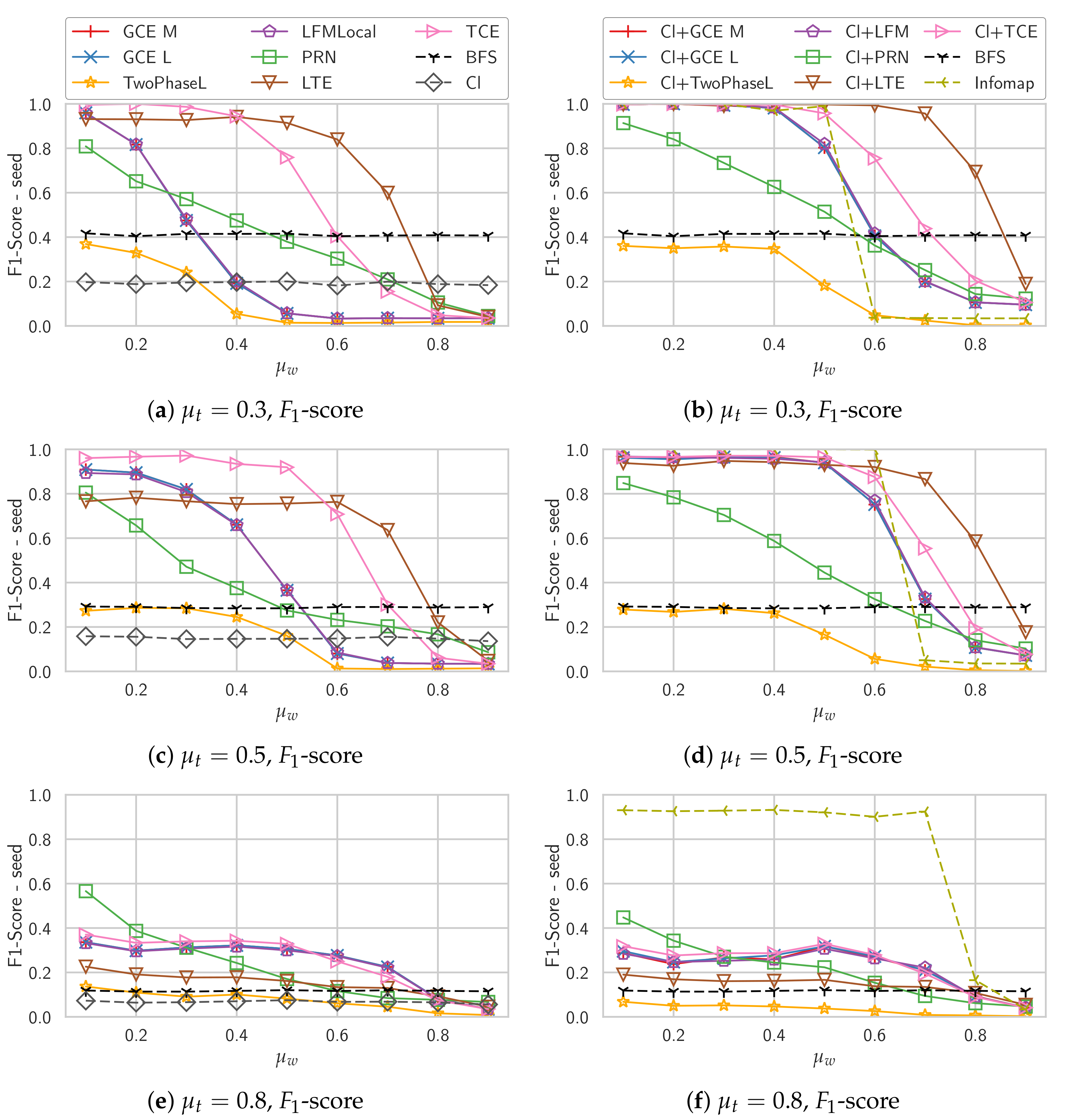
Figure 1 shows the average -scores both for the variants starting from a single seed node (left column) as well as when starting from the maximum clique (right column). The “Cl” algorithm in the left column is just the maximum clique of the seed node, i.e., the starting point of the algorithms in the right column.
The performance of the plain Local T algorithm is well below the performance of the baseline BFS, with clique initialization it performs slightly better but still worse than all other algorithms. Even the simple clique algorithm outperforms it in terms of score. The density-based simple greedy expansion algorithms GCE M, GCE L and LFM all perform very similar, which is not unexpected as they are based on very similar quality functions. With a clique as initialization their performance is significantly improved, in particular on the smaller communities they return almost perfect communities even past . The original L-based community detection algorithm, Two-Phase L, performs worse than these simple expansion algorithms. One explanation for this behavior is that if the seed node is no longer part of the detected community, the algorithm simply returns an empty community, giving a score of 0. Only the triangle-based algorithms LTE and TCE perform well when initialized with a single seed node. They also profit from the initialization with a clique, though. In particular on the smaller communities their performance is not far from the Infomap algorithm, which is able to perfectly recover the community structure till . The PageRank-Nibble algorithm (PRN) performs only well on the graphs with low values of , for higher values its performance degrades very quickly.
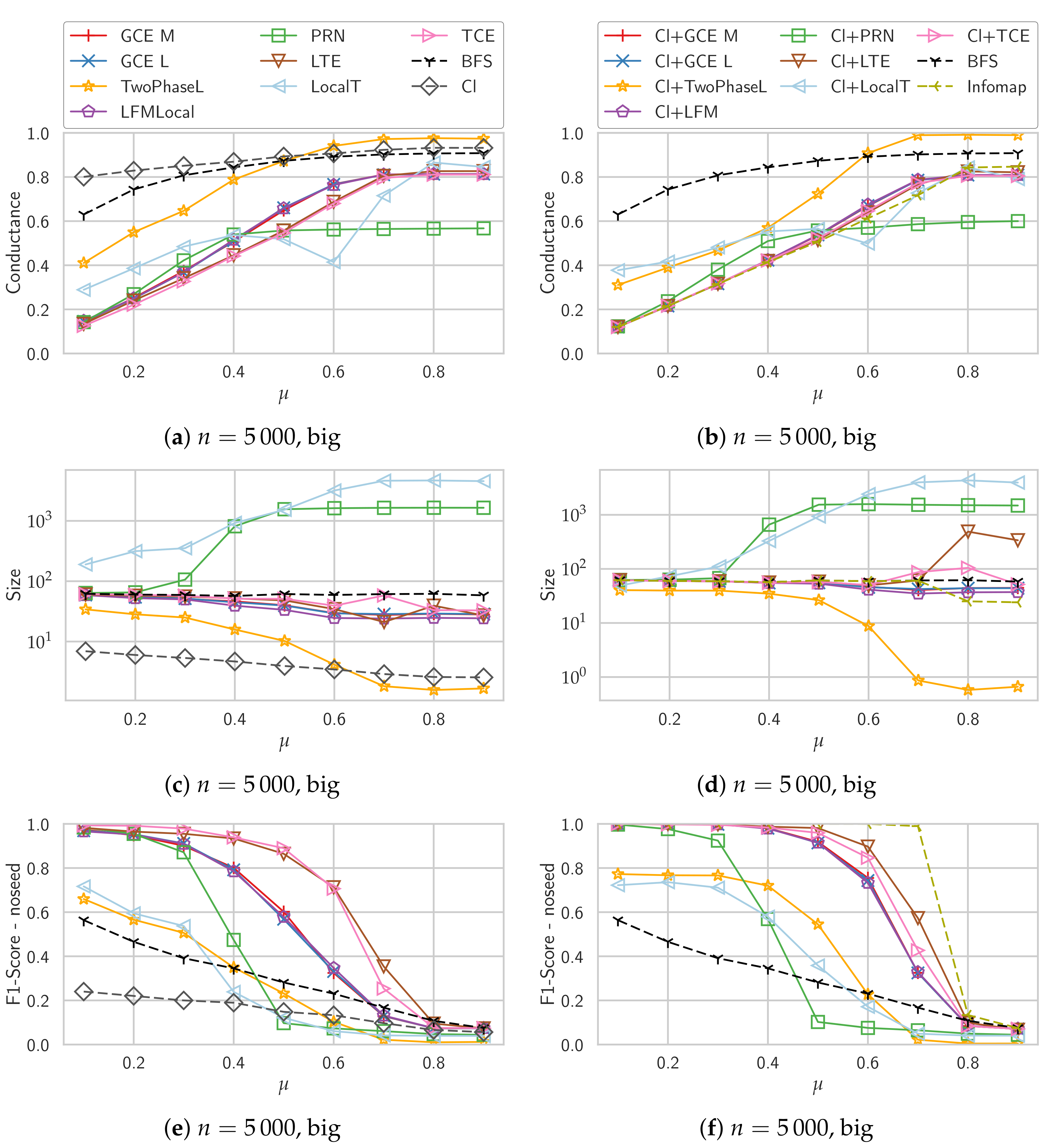
To explore the performance of the different algorithms in more detail and get some explanations for their behavior, we show more detailed results in Figure 2. In Figure 2a,b, we see the conductance of the detected communities. Due to the definition of conductance and the ground truth communities in LFR, corresponds exactly to the conductance of the ground truth communities. We can see here that the triangle-based algorithms which almost perfectly recover the community structure (TCE and LTE) also yield good, though not perfect conductance values. For the methods based on density and simple greedy expansion, GCE M, GCE L, LFMLocal, we can see that the coductance of the detected communities is improved by starting from a clique.
PageRank-Nibble shows an interesting behavior here: starting with , the conductance stays almost the same, i.e., is better than what the other algorithms find. Looking at Figure 2c,d which show the sizes of the detected communities, we can see that PageRank-Nibble finds really large communities that, starting with contain almost half of the nodes of the whole graph. The explanation for this is that if you randomly cut a graph in two parts equally-sized parts, in expectation you also split the neighbors of every node in two equally-sized parts. Therefore, for every node u in expectation about half of u’s neighbors are in the same part as u and the other half is in the other part. This yields a conductance of 0.5. Therefore, if the initial local PageRank approximation visits enough nodes, a large enough prefix of the sorted nodes will have a lower conductance than the actual community. Further, if the actual community is not perfectly detected, its conductance is higher and therefore the effect starts already around .
The Local T algorithm consistently finds way too large communities that also have high conductance values except for some range around , where probably the community size is just right to get low conductance values regardless of the chosen cut.
Concerning the sizes, the density-based algorithms GCE M, GCE L and LFM as well as TCE and LTE find approximately the right size, though for larger communities they tend to discover too few nodes. Starting with a clique improves this, the detected community sizes now rather correspond to the correct size which is always returned by the BFS baseline by design. Only LTE then tends to detect too large communities for where the community structure cannot be recovered anymore.
For Two-Phase L we can clearly see that above , the algorithm finds smaller and smaller communities on average, meaning that more and more often it decides that the detected community is no community and discards it.
In Figure 2e,f we report the average score of every detected community with the best ground truth community regardless if that community contains the seed node. For GCE M, GCE L and LFM we can clearly see that they get much better scores compared to the comparison considering only the ground truth community of the seed node. This shows that these algorithms find communities in which the seed node is not strongly embedded. For the algorithms starting with a clique, this effect is much weaker, though for higher values of it is visible for all algorithms. Existing work frequently ignores this e.g., by just considering the cover that is detected by iteratively applying the algorithm to nodes that do not yet belong to a community [5,15].
4.4. Overlapping Communities
Our parameter set for overlapping communities is inspired by the highly overlapping parameter set used in [8]. All nodes belong to the same number of communities which is in the range . We modified the parameters slightly by not setting the average degree but the minimum degree to . This has the effect that the minimum internal degree of a community stays the same with increasing values of . Using NetworKit, we calculated the expected average degree for this minimum degree and used these as parameters for the LFR generator.
Figure 3 shows the results for these networks. Note that here we do not evaluate if an algorithm is able to discover all or a specific community of a node, we compare to the community of the seed node that is best matched. The performance of LocalT is extremely poor, it cannot detect any overlapping communities and without a clique as initialization, it cannot even detect the non-overlapping communities. PageRank-Nibble is also unable to discover any communities starting for , which is not really surprising as the PageRank approximation has no way to decide for one of the communities of the seed node. The other algorithms perform better, LTE being best when starting without a clique. The largest clique of the seed node as initialization again improves the performance, and, quite interestingly, when starting with a clique, the density-based algorithms GCE M, GCE L and LFM perform better than the triangle-based algorithms LTE and TCE. A possible explanation for this could be that triangles are less helpful in the case of overlapping communities as a node can have triangles with neighbors of any community. Infomap completely fails to discover the overlapping community structure, but this is expected as we only used the variant for disjoint communities.
Weighted Graphs
For the weighted graphs, we use the parameter set “Weighted” in Table 1, those are the parameters also used by Lancichinetti et al. [11]. This means that we have a single community size range, . We further choose three values for the topological mixing parameter . The weight mixing parameter is varied from 0.1 to 0.9 in each of these sets. For each we generate 20 instances and run the algorithms from 20 randomly chosen seed nodes.
For the weighted graphs, we do not compare LocalT as it only works on unweighted graphs and it is not clear how to generalize it to weighted graphs, the authors discuss this as future work. In Figure 4 we show the results for the other algorithms. For each value of the topological mixing parameter we plot the weight mixing parameter on the x-axis and the resulting average score on the y-axis.
Comparing the two plots at and , we can see that while most algorithms even improve their performance at , LTE has a worse performance. A possible explanation for this is that its score of the community is based on the presence of triangles. While TCE is also based on triangles for the decision which node to add next, its score of the community is solely based on the density and should thus be independent of the structure of the graph as long as the weights are correctly distributed. This can be seen by its performance which is even better for . When initialized with a clique, LTE has fewer problems though and even outperforms Infomap for high values of . This is probably due to its community score being based on the structure of the graph and thus taking weights less into account. Two-Phase L performs worse than our baseline BFS, apparently the two-phase process is not so suited for this kind of weighted graph. The other density-based algorithms GCE M, GCE L and LFM perform similarly for unweighted graphs.
For , none of the algorithms is able to accurately detect the community structure anymore. This is most likely due to the low intra-community degree. Note that the chosen values of and result in a minimum degree of 10, which means that at , the low-degree nodes have only two neighbors in their own community. PageRank-Nibble seems to be least affected by this, though its performance is also significantly worse than for . LTE performs worse than the other algorithms as it is most affected by the lack of triangles. Cliques also do not help anymore, this is most likely also due to the low internal degree. The still good performance of Infomap shows, though, that in principle the community structure is still detectable.
4.5. Facebook Graphs
The synthetic graphs of benchmarks, like LFR, are an excellent way to compare algorithms and can show their quality. However, good performance on synthetic graphs does not necessarily translate to good performance on real world graphs. Good performance on real world graphs is also an important quality of algorithms. After all, we design our algorithms with the goal in mind to be able to find communities on real graphs. Therefore, we test and evaluate the algorithms here on real world social networks.
The Facebook 100 data set was first published by Traud et al. [34]. It consists of 100 graphs, which are snapshots from September 2005. Each of these graphs describes the social network of Facebook at a university or college and is restricted to that university/college. The graph of a university or college consists of the persons, who work, study, or studied there. Unweighted edges between persons (nodes) exist, if they are friends on Facebook and the nodes have attributes, like graduation year, dormitory, major and high school. It has been shown that at least for some of the graphs there are correlations between edges and the attributes dormitory and graduation year [34]. The Facebook graphs are therefore frequently used in testing and comparing algorithms on real world data by looking at the correlations with their attributes [4,8,37]. We compare against the community structure induced by the dormitories. These are not ground truth communities, though. Therefore, our results only show how well the communities detected by the algorithms and the attribute correlate. This has many flaws, one of them being that the attribute is missing for some nodes. Another is that the subgraph induced by one of the attribute values is not necessarily connected, in preliminary tests we found that they often even consist of more than two connected components. As these flaws affect all algorithms equally, we still consider this a valid evaluation.
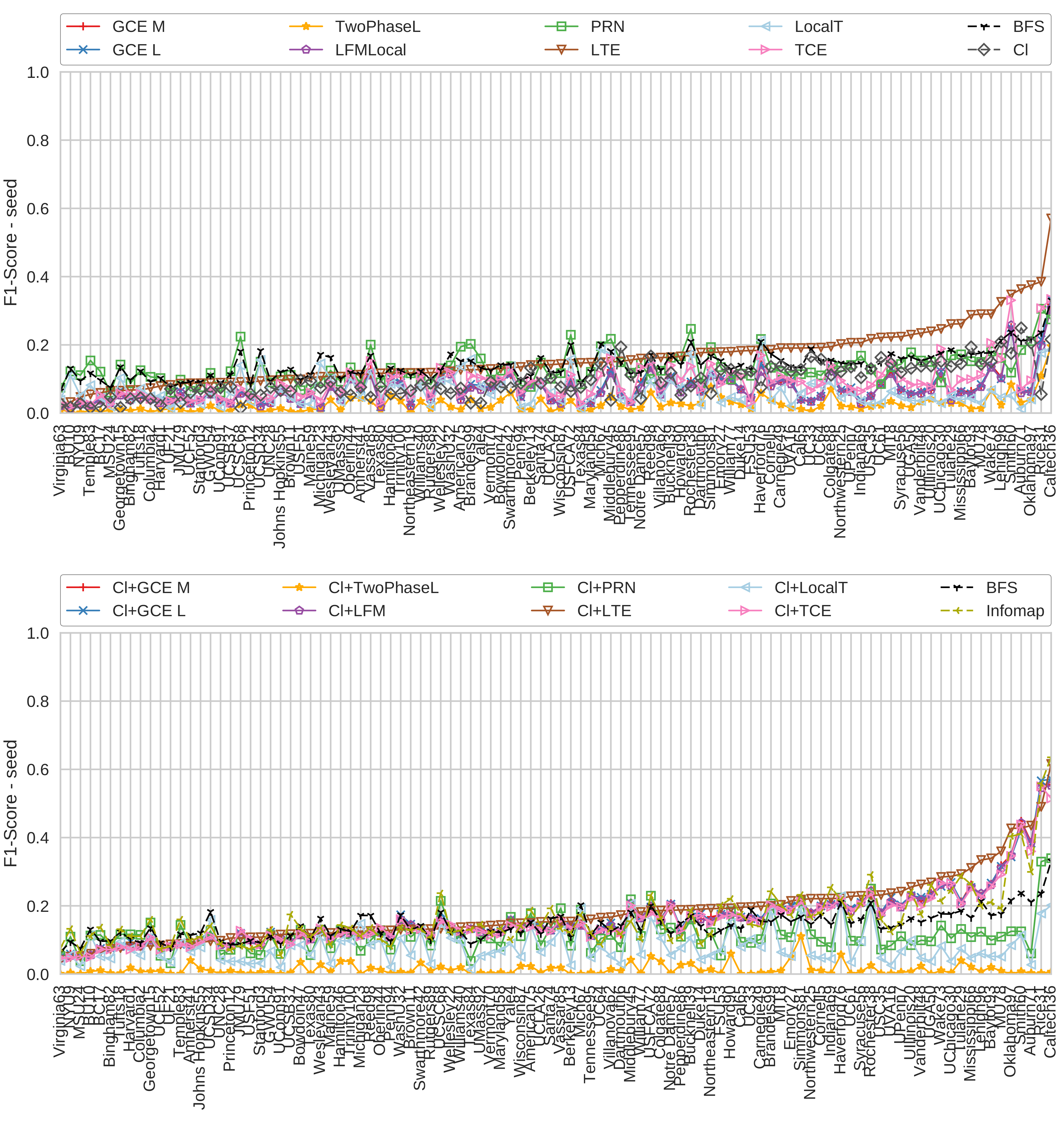
We pick 100 random nodes as seed nodes on each graph and execute the algorithms for each of them. When picking the seed nodes, we ensure that each of them has the dormitory attribute set. Figure 5 shows the resulting -scores for all 100 graphs, which we sorted after the -score of LTE.
Clearly, LTE is the best-performing algorithm, in particular when starting with a single seed node. There, on most graphs, none of the other algorithms even exceeds the performance of the baseline BFS. When starting from the maximum clique, TCE, GCE M, GCE L and LFM perform much better and now better than the BFS baseline on many graphs but still worse than LTE. LTE also profits from starting from a clique, but only slightly. PageRank-Nibble does not seem to profit from the clique at all, it appears rather that results are becoming worse when starting from a clique. The Two-Phase L algorithm often decides that no community was discovered, on some of the graphs it even decided that for all 100 seed nodes. While Infomap is among the better algorithms, it does not outperform LTE on most of the graphs.
4.6. Running Times
In Table 2 we present the running times (wall time) and detected community sizes of the local community detection algorithms averaged over all 100 Facebook graphs and over the overlapping LFR benchmark graphs. While they show different rankings, one can still find some similarities. First of all, LocalT is the slowest algorithm by a large margin and returns the largest communities. LTE is second-slowest, followed by TCE on the LFR graphs. A main difference between the Facebook and the LFR graphs is the time required for listing all maximal cliques. While it is really fast on the LFR graphs, it is slower than executing executing any local community detection algorithm apart from LTE and LocalT on the Facebook networks. A possible explanation could be the different structure of the Facebook networks with larger cliques and higher degrees, though the average clique size on the Facebook networks is with 14 only twice as large as the average on the LFR graphs, which is 7. PageRank-Nibble is quite fast on both types of networks, closely followed by the simple expansion strategies GCE M and GCE L. LFM with the more advanced removal strategy is slightly slower. The Two-Phase L algorithm is the fastest algorithm on the Facebook networks, but there it also hardly finds communities so probably it does not only find communities without the seed node as we saw in earlier experiments but the expansion also stops early on these networks. On the LFR benchmark where the performance was similar to the simpler density-based algorithms, Two-Phase L is slightly slower than these algorithms but still faster than the triangle-based algorithms.
4.7. Summary
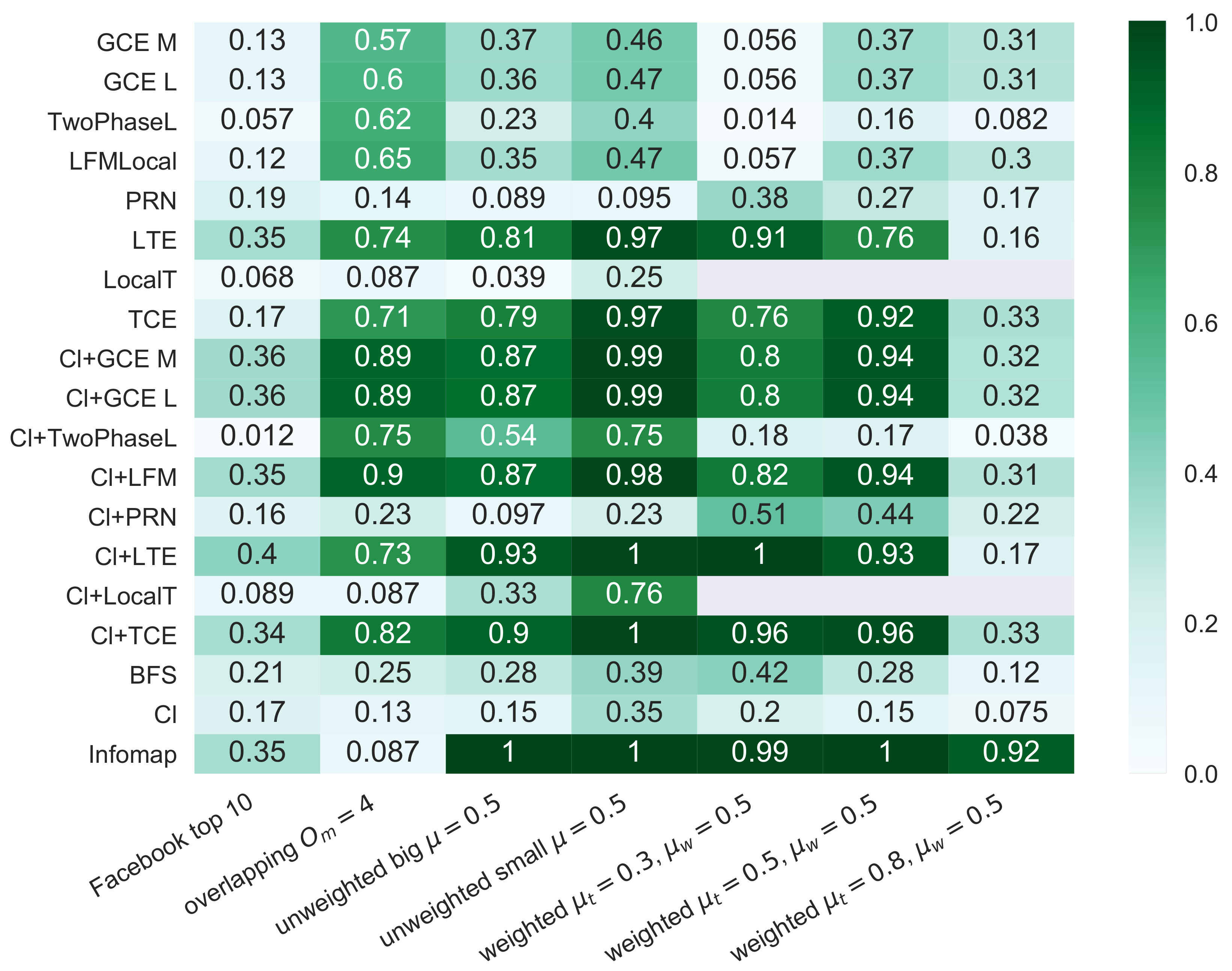
In Figure 6 we summarize the experimental results concerning the quality of the found communities. For each type of LFR graph with non-overlapping communities, we show the result for as this is for all graphs a value where many algorithms still find reasonable results but differences between algorithms are already visible. For LFR graphs with overlapping communities we picked 4 communities per node for the same reason. For the set of 100 Facebook graphs we report the average over the 10 graphs where LTE starting with a clique (the best-performing algorithm according to our results) found the best-matching communities. On all considered types of graphs, the algorithms not starting with a clique perform worse than those starting with a clique, though LTE and TCE still show reasonable results for many graphs. The algorithms TwoPhaseL, PageRank-Nibble and LocalT perform worse than the other algorithms on all types of graphs. On unweighted LFR graphs and on the Facebook graphs, LTE with clique initialization wins. However, with overlapping communities and with edge weights and a not so clear structure (i.e., ), it seems its triangle-based score is more easily confused and outperformed by the simpler density-based algorithms like LFM or GCE with clique initialization. Our newly proposed TCE algorithm is between them, on weighted LFR graphs it is even among the best-performing algorithms. Compared to the global, non-overlapping Infomap algorithm the results are quite competitive, only on the weighted graphs Infomap performs significantly better. On the Facebook networks, the performance of Infomap is even inferior to some local algorithms. For the overlapping LFR networks, Infomap correctly finds that there is no good non-overlapping community structure.
Overall, these results show that while using a clique as initialization is beneficial on all types of graphs, the choice of the expansion algorithm should always depend on the type of the graph. For weighted graphs, it can be dangerous to depend too much on the structure of the graph as LTE does. For LFR graphs with a highly overlapping community structure, methods solely based on the density outperform those based on triangles which is a bit surprising as one would still expect that intra-cluster edges are structurally more embedded. This could mean that possibly scores based on triangles are not as sophisticated as those based on density and should be further improved.
5. Conclusions
We have compared a set of 8 local community detection algorithms, one of them—Triangle Based Community Expansion—being a novel algorithm. For the evaluation we used both synthetically generated benchmark graphs and real-world social networks. We have shown that triangle-based algorithms are superior to solely density-based algorithms, in particular on real-world networks. Further, we have shown that all algorithms benefit from not starting from a single seed node but the maximum clique in the neighborhood of the seed node.
Algorithms based on triangles could also be used to improve global overlapping community detection algorithms such as GCE [8]. In the case of global algorithms, the pre-computation of edge scores and using more efficient arrays instead of hash tables led to significant speedups as preliminary experiments indicate. Further, our approach could also be extended to dynamic graphs, possibly using a similar approach to [38]. Data structures for maintaining triangle counts [31,39] could thereby be used to update edge and node scores.
Acknowledgments
This work was partially supported by the DFG under grant WA 654/22-2.
Author Contributions
M.H. did most of the work concerning the concept, the used implementation, the execution and evaluation of the experiments and the writeup. E.R. designed, implemented and evaluated a preliminary version of the experiments and contributed to the writeup. D.W. was involved in the concept of the study and the proof reading of the writeup.
Conflicts of Interest
The authors declare no conflict of interest.
References
- Fortunato, S. Community detection in graphs. Phys. Rep. 2010, 486, 75–174. [Google Scholar] [CrossRef]
- Fortunato, S.; Hric, D. Community detection in networks: A user guide. Phys. Rep. 2016, 659, 1–44. [Google Scholar] [CrossRef]
- Schaeffer, S.E. Graph clustering. Comput. Sci. Rev. 2007, 1, 27–64. [Google Scholar] [CrossRef]
- Staudt, C.; Marrakchi, Y.; Meyerhenke, H. Detecting communities around seed nodes in complex networks. In Proceedings of the IEEE International Conference on Big Data, Washington, DC, USA, 27–30 October 2014; pp. 62–69. [Google Scholar]
- Lancichinetti, A.; Fortunato, S.; Kertész, J. Detecting the overlapping and hierarchical community structure of complex networks. New J. Phys. 2009, 11. [Google Scholar] [CrossRef]
- Lancichinetti, A.; Radicchi, F.; Ramasco, J.J.; Fortunato, S. Finding Statistically Significant Communities in Networks. PLoS ONE 2011, 6, 1–18. [Google Scholar] [CrossRef] [PubMed]
- McDaid, A.; Hurley, N. Using Model-based Overlapping Seed Expansion to detect highly overlapping community structure. arXiv 2010, arXiv:1011.1970. [Google Scholar]
- Lee, C.; Reid, F.; McDaid, A.; Hurley, N. Detecting highly overlapping community structure by greedy clique expansion. arXiv 2010, arXiv:1002.1827. [Google Scholar]
- Fanrong, M.; Mu, Z.; Yong, Z.; Ranran, Z. Local Community Detection in Complex Networks Based on Maximum Cliques Extension. Mathe. Probl. Eng. 2014, 2014, 653670. [Google Scholar] [CrossRef]
- Radicchi, F.; Castellano, C.; Cecconi, F.; Loreto, V.; Parisi, D. Defining and identifying communities in networks. Proc. Natl. Acad. Sci. USA 2004, 101, 2658–2663. [Google Scholar] [CrossRef] [PubMed]
- Lancichinetti, A.; Fortunato, S. Community detection algorithms: A comparative analysis. Phys. Rev. E 2009, 80, 056117. [Google Scholar] [CrossRef] [PubMed]
- Lancichinetti, A.; Fortunato, S. Benchmarks for testing community detection algorithms on directed and weighted graphs with overlapping communities. Phys. Rev. E 2009, 80, 016118. [Google Scholar] [CrossRef] [PubMed]
- Staudt, C.; Sazonovs, A.; Meyerhenke, H. NetworKit: A tool suite for large-scale complex network analysis. Netw. Sci. 2016, 4, 508–530. [Google Scholar] [CrossRef]
- Hamann, M.; Röhrs, E.; Wagner, D. Local Community Detection Based on Small Cliques: Implementation and Evaluation Scripts. GitHub 2017. Available online: https://github.com/kit-algo/LCD-cliques-experiments (accessed on 10 August 2017).
- Huang, J.; Sun, H.; Liu, Y.; Song, Q.; Weninger, T. Towards Online Multiresolution Community Detection in Large-Scale Networks. PLoS ONE 2011, 6, e23829. [Google Scholar] [CrossRef] [PubMed]
- Clauset, A. Finding local community structure in networks. Phys. Rev. E 2005, 72, 026132. [Google Scholar] [CrossRef] [PubMed]
- Chen, J.; Zaïane, O.R.; Goebel, R. Local Community Identification in Social Networks. In Proceedings of the 2009 IEEE/ACM International Conference on Advances in Social Networks Analysis and Mining, Athens, Greece, 20–22 July 2009; pp. 237–242. [Google Scholar]
- Bagrow, J.P. Evaluating local community methods in networks. J. Stat. Mech. Theory Exp. 2008, 2008, P05001. [Google Scholar] [CrossRef]
- Fagnan, J.; Zaiane, O.; Barbosa, D. Using triads to identify local community structure in social networks. In Proceedings of the 2014 IEEE/ACM International Conference on Advances in Social Networks Analysis and Mining (ASONAM), Beijing, China, 17–20 August 2014; pp. 108–112. [Google Scholar]
- Ngonmang, B.; Tchuente, M.; Viennet, E. Local Community Identification in Social Networks. Parallel Process. Lett. 2012, 22, 1240004. [Google Scholar] [CrossRef]
- Ma, L.; Huang, H.; He, Q.; Chiew, K.; Liu, Z. Toward seed-insensitive solutions to local community detection. J. Intell. Inf. Syst. 2014, 43, 183–203. [Google Scholar] [CrossRef]
- Andersen, R.; Chung, F.; Lang, K. Local Graph Partitioning using PageRank Vectors. In Proceedings of the 47th Annual IEEE Symposium on Foundations of Computer Science (FOCS’06), Berkeley, CA, USA, 21–24 October 2006; pp. 475–486. [Google Scholar]
- Panagiotakis, C.; Papadakis, H.; Fragopoulou, P. Local Community Detection via Flow Propagation. In Proceedings of the 2015 IEEE/ACM International Conference on Advances in Social Networks Analysis and Mining, Paris, France, 25–28 August 2015; pp. 81–88. [Google Scholar]
- Li, Y.; He, K.; Bindel, D.; Hopcroft, J.E. Uncovering the small community structure in large networks: A local spectral approach. In Proceedings of the 24th International Conference on World Wide Web, Florence, Italy, 18–22 May 2015; pp. 658–668. [Google Scholar]
- Danisch, M.; Guillaume, J.L.; Grand, B.L. Towards multi-ego-centred communities: A node similarity approach. Int. J. Web Based Communities 2013, 9, 299–322. [Google Scholar] [CrossRef]
- Jia, S.; Gao, L.; Gao, Y.; Wang, H. Anti-triangle centrality-based community detection in complex networks. Syst. Biol. IET 2014, 8, 116–125. [Google Scholar] [CrossRef] [PubMed]
- Watts, D.J.; Strogatz, S.H. Collective dynamics of ‘small-world’networks. Nature 1998, 393, 440–442. [Google Scholar] [CrossRef] [PubMed]
- Easley, D.; Kleinberg, J. Networks, Crowds, and Markets: Reasoning about a Highly Connected World; Cambridge University Press: Cambridge, UK, 2010. [Google Scholar]
- Luo, F.; Wang, J.Z.; Promislow, E. Exploring local community structures in large networks. Web Intell. Agent Syst. An Int. J. 2008, 6, 387–400. [Google Scholar]
- Yang, J.; Leskovec, J. Defining and evaluating network communities based on ground-truth. Knowl. Inf. Syst. 2015, 42, 181–213. [Google Scholar] [CrossRef]
- Lin, M.C.; Soulignac, F.J.; Szwarcfiter, J.L. Arboricity, h-index, and dynamic algorithms. Theor. Comput. Sci. 2012, 426, 75–90. [Google Scholar] [CrossRef]
- Eppstein, D.; Löffler, M.; Strash, D. Listing All Maximal Cliques in Large Sparse Real-World Graphs. ACM J. Exp. Algorithm. 2013, 18. [Google Scholar] [CrossRef]
- Eppstein, D.; Löffler, M.; Strash, D. Listing All Maximal Cliques in Sparse Graphs in Near-Optimal Time. In International Symposium on Algorithms and Computation; Lecture Notes in Computer Science; Springer: Berlin/Heidelberg, Germany, 2010; pp. 403–414. [Google Scholar]
- Traud, A.L.; Mucha, P.J.; Porter, M.A. Social Structure of Facebook Networks. arXiv 2011, arXiv:1102.2166. [Google Scholar]
- Rosvall, M.; Axelsson, D.; Bergstrom, C.T. The map equation. Eur. Phys. J. Spec. Top. 2009, 178, 13–23. [Google Scholar] [CrossRef]
- Yang, J.; Leskovec, J. Structure and overlaps of ground-truth communities in networks. ACM Trans. Intell. Syst. Technol. 2014, 5, 26. [Google Scholar] [CrossRef]
- Lee, C.; Cunningham, P. Benchmarking community detection methods on social media data. arXiv 1302. [Google Scholar]
- Zakrzewska, A.; Bader, D.A. A Dynamic Algorithm for Local Community Detection in Graphs. In Proceedings of the 2015 IEEE/ACM International Conference on Advances in Social Networks Analysis and Mining, Paris, France, 25–28 August 2015; pp. 559–564. [Google Scholar]
- Eppstein, D.; Spiro, E.S. The h-Index of a Graph and Its Application to Dynamic Subgraph Statistics. In Proceedings of the WADS’09 11th International Symposium on Algorithms and Data Structures, Banff, AB, Canada, 21–23 August 2009; Lecture Notes in Computer Science. Dehne, F., Gavrilova, M., Sack, J.R., Tóth, C.D., Eds.; Springer: Berlin/Heidelberg, Germany, 2009; Volume 5664, pp. 278–289. [Google Scholar]
Figure 1.
Avg. -scores on the LFR benchmark with the parameter set Unweighted, which we specify in Table 1. The left column shows results when starting with a single seed node, the right column shows results for starting with the maximum clique as well as Infomap for comparison.
Figure 1.
Avg. -scores on the LFR benchmark with the parameter set Unweighted, which we specify in Table 1. The left column shows results when starting with a single seed node, the right column shows results for starting with the maximum clique as well as Infomap for comparison.
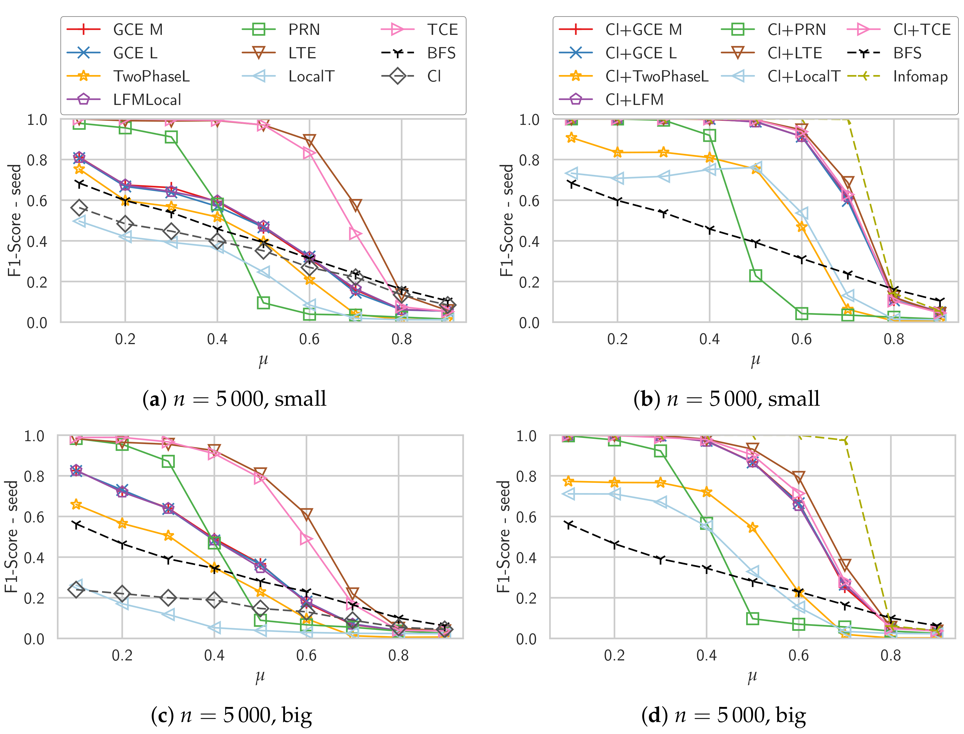
Figure 2.
Different measures for the 5000 node unweighted graph with disjoint big communities.

Figure 3.
Results for overlapping communities with LFR graphs with parameter set “Overlapping” as specified in Table 1.
Figure 3.
Results for overlapping communities with LFR graphs with parameter set “Overlapping” as specified in Table 1.
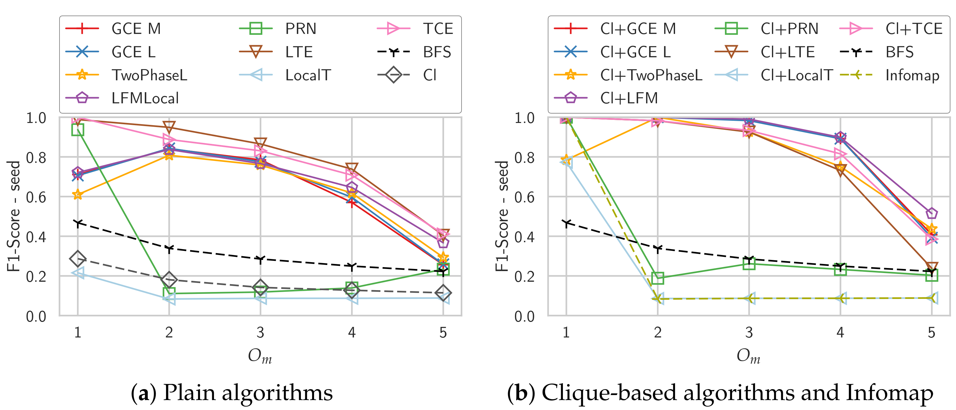
Figure 4.
Avg. -scores on the LFR benchmark with the parameter set Weighted, as specified in Table 1.
Figure 4.
Avg. -scores on the LFR benchmark with the parameter set Weighted, as specified in Table 1.

Figure 5.
Average -scores of the algorithms on all 100 Facebook graphs. The scores are calculated by treating the dormitory attribute as communities. The graphs are sorted by the -score of CCE.
Figure 5.
Average -scores of the algorithms on all 100 Facebook graphs. The scores are calculated by treating the dormitory attribute as communities. The graphs are sorted by the -score of CCE.

Figure 6.
Summary of F1-Score - seed values of all types of networks considered. The results for the Facebook networks are averages over the 10 networks where “Cl+LTE” had the best scores. LocalT does not support edge weights and is therefore omitted for weighted graphs.
Figure 6.
Summary of F1-Score - seed values of all types of networks considered. The results for the Facebook networks are averages over the 10 networks where “Cl+LTE” had the best scores. LocalT does not support edge weights and is therefore omitted for weighted graphs.

Table 1.
Parameters of the LFR benchmark that we use in our experiments.
| Name | Description | Unweighted | Overlapping | Weighted |
|---|---|---|---|---|
| n | number of nodes | 5000 | 2000 | 5000 |
| k | average degree | 20 | 39.5, 61.5, 78.1, 91.8, 103.5 | 20 |
| maximum degree | 50 | 120 | 50 | |
| degree exponent | ||||
| minimum community size | 10, 20 | 60 | 20 | |
| maximum community size | 50, 100 | 120 | 100 | |
| community size exponent | ||||
| topological mixing | 0.1, …, 0.9 | 0.2 | 0.3, 0.5, 0.8 | |
| weight exponent | ||||
| weight mixing | 0.1, …, 0.9 | |||
| communities per node | 1 | 1, ..., 5 | 1 |
Table 2.
Average times (ms) per seed node and average community sizes of the algorithms.
| (a) On the Overlapping LFR Benchmark. | (b) On the 100 Facebook Networks. | ||||
|---|---|---|---|---|---|
| Size | Time (ms) | Size | Time (ms) | ||
| Cl | 7 | 0.4 | TwoPhaseL | 38 | 1.7 |
| Cl+PRN | 419 | 2.1 | PRN | 975 | 4.2 |
| PRN | 605 | 2.9 | GCE M | 282 | 5.9 |
| Cl+GCE M | 321 | 3.5 | GCE L | 270 | 6.7 |
| GCE M | 405 | 3.7 | LFMLocal | 221 | 9.8 |
| Cl+GCE L | 333 | 4.0 | TCE | 321 | 11.4 |
| GCE L | 411 | 4.4 | Cl | 14 | 13.0 |
| LFMLocal | 249 | 4.8 | Cl+TwoPhaseL | 52 | 17.5 |
| Cl+LFM | 242 | 5.1 | Cl+PRN | 1086 | 18.5 |
| Cl+TwoPhaseL | 243 | 5.3 | Cl+GCE M | 1009 | 45.1 |
| TwoPhaseL | 329 | 6.8 | Cl+TCE | 930 | 46.5 |
| TCE | 320 | 10.2 | Cl+GCE L | 919 | 48.0 |
| Cl+TCE | 320 | 10.5 | Cl+LFM | 907 | 77.4 |
| LTE | 294 | 26.4 | LTE | 257 | 107.5 |
| Cl+LTE | 436 | 28.8 | Cl+LTE | 407 | 150.5 |
| LocalT | 1618 | 49.7 | LocalT | 8066 | 1028.1 |
| Cl+LocalT | 1589 | 49.7 | Cl+LocalT | 8207 | 1054.7 |
© 2017 by the authors. Licensee MDPI, Basel, Switzerland. This article is an open access article distributed under the terms and conditions of the Creative Commons Attribution (CC BY) license (http://creativecommons.org/licenses/by/4.0/).
Share and Cite
MDPI and ACS Style
Hamann, M.; Röhrs, E.; Wagner, D. Local Community Detection Based on Small Cliques. Algorithms 2017, 10, 90. https://doi.org/10.3390/a10030090
AMA Style
Hamann M, Röhrs E, Wagner D. Local Community Detection Based on Small Cliques. Algorithms. 2017; 10(3):90. https://doi.org/10.3390/a10030090
Chicago/Turabian StyleHamann, Michael, Eike Röhrs, and Dorothea Wagner. 2017. "Local Community Detection Based on Small Cliques" Algorithms 10, no. 3: 90. https://doi.org/10.3390/a10030090
Note that from the first issue of 2016, this journal uses article numbers instead of page numbers. See further details here.