Predictive Current Control of Boost Three-Level and T-Type Inverters Cascaded in Wind Power Generation Systems


1
Electrical Engineering College, Yanshan University, Qinhuangdao 066004, China
2
The Department of Mechanical and Electronic Engineering, Bayin Guoleng Vocational and Technical College, Korla 841000, China
3
Department of Energy Technology, Aalborg University, 9220 Aalborg, Denmark
*
Author to whom correspondence should be addressed.
Algorithms 2018, 11(7), 92; https://doi.org/10.3390/a11070092
Submission received: 7 May 2018
/
Revised: 14 June 2018
/
Accepted: 25 June 2018
/
Published: 27 June 2018
Abstract
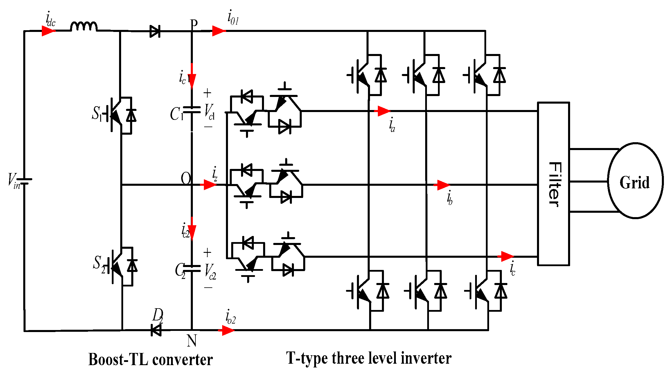
:A topology structure based on boost three-level converters (BTL converters) and T-type three-level inverters for a direct-drive wind turbine in a wind power generation system is proposed. In this structure, the generator-side control can be realized by the boost-TL converter. Compared with the conventional boost converter, the boost-TL converter has a low inductor current ripple, which reduces the torque ripple of the generator, increases the converter’s capacity, and minimizes switching losses. The boost-TL converter can boost the DC output from the rectifier at low speeds. The principles of the boost-TL converter and the T-type three-level inverter are separately introduced. Based on the cascaded structure of the proposed BTL converter and three-level inverter, a model predictive current control (MPCC) method is adopted, and the optimization of the MPCC is presented. The prediction model is derived, and the simulation and experimental research are carried out. The results show that the algorithm based on the proposed cascaded structure is feasible and superior.
1. Introduction
In a wind power generation system (WPGS) scheme, rectifiers are used to extract power from a renewable energy source in a controlled manner [1], which is then delivered to the grid by means of a voltage source inverter (VSI). The most commonly used topology for this application is the back-to-back converter, which achieves bidirectional power flow [2]. Nevertheless, when bidirectionality is not needed, using an uncontrolled rectifier + three level boost chopper represents a cheaper alternative than the former.
Three level boost chopper has a large number of advantages compared with the conventional boost converter, such as: (a) comparing to the previous boost converter, the inductor current ripple of the boost-TL converter is lower, reducing the generator torque ripple; (b) the voltage stress of the power device is less than that of the conventional boost converter, so the output voltage of the generator and the capacity of the converter can both be increased; (c) in the case of the same inductor current, the switching frequency is half that of the conventional boost converter, so the switching losses are less; (d) the boost-TL converter boosts the DC output voltage from the rectifier at low speeds, so it also allows the wind power generator to operate over a wider speed range. Therefore, the boost three-level converter is widely adopted in modern power electronics apparatus. In [3], the MPPT and the methods of the voltage balancing control for the boost three-level converter are proposed, however, MPC is not adopted. In [4], a novel predictive controller for a series-interleaved multicell boost three-level PFC converter has been presented.
In wind power generation systems, multilevel converter topology has received increasing attention in order to meet the ever-increasing stand-alone capacity of wind turbine generators and the ever-increasing current and voltage levels of converters. The neutral-point-clamped (NPC) inverter and T-type inverter are commonly adopted in the three-level inverter topology, compared with the NPC inverter, the T-type three-level structure also has many advantages, such as: (a) small number of components; (b) the control signal has no stop sequence problem and is easier to control; (c) low switching loss and high efficiency; (d) less driving power; and (e) in the aspect of the commutation path, the conversion paths between the outer tube Sa1/Sa2 and the inner tube Sa3/Sa4 are all the same, and the problems of the stray inductance and the voltage peak are less.
With the development of wind power systems, the converter circuit of uncontrolled rectifier + boost chopper + PWM inverter has attracted more and more interest of scholars from various countries. In the circuit, the rectifier part adopts a diode uncontrolled rectifier, the boost converter in the middle DC link raises the DC voltage, and the inverter part adopts a PWM three-phase bridge inverter. Compared with back-to-back PWM converters, the topology of the generator-side converter has been simplified, a number of power switch devices and their driving circuits are omitted, the switching loss of the power device is reduced, the cost is reduced, and the reliability of the whole system is enhanced.
Combining the advantages mentioned earlier, a topology based on boost three-level converter (BTL converter) and T-type three-level inverter cascaded for wind power generation system is proposed, as shown in Figure 1.
Since FCS-MPC has an intuitive concept, flexible control, no modulator, no parameter setting, and fast dynamic response, it can also effectively deal with the system of non-linear links and various restrictions and other advantages, so it has become a hot research topic. At present, FCS-MPC has been widely used in various power electronic converters. Compared with proportional integral control, MPC has superior performance and has attracted much attention. First presented in [5], MPC deals with linear and nonlinear models and provides maximum realizable bandwidth. For the boost converter, the predictive control method has been deeply studied. Reference [6] Yaramasu, V. and Wu, B. adopted predictive control of BTL using a dynamic model of inductance current and DC bus voltage. Adopted regression methods in [7] to predict the next cycle current of digital controller delay compensation by Baggio, J., etc. In [8], the FCS-MPC method is adopted to reduce the CMV and balance the NP voltage with fast dynamics of the three-level T-type inverter by Xing, X., etc. In [9], the modified model predictive control algorithm for the high efficiency with reduced switch stress t-type three-level inverter with the neutral point clamped is presented by Abdel-Rahim, O., etc. In [10], a radial basis function neural network optimization model predictive control (MPC) was proposed by Han, B., etc. for large wind turbines, which meets the requirements of the specified operation region. Reference [11] Wang, X. and Sun, D proposes a three-vector-based low complexity model predictive direct power control strategy for doubly-fed induction generators (DFIGs) in wind energy applications, which improve the steady-state performance and achieves error-free control. In [12], the proposed sensorless method by Bayhan, S., etc. offers as a model-free solution, the MPC strategy has been used as a current controller to overcome the weaknesses of the inner control loop and considers the discrete-time operation of the VSC.
In this paper, a new predictive current control method without any kind of linear controller or modulation technology is proposed for the BTL and three-level T-type inverter cascaded topology, with stable performance of THD improved significantly.
The structure of this paper is organized as follows: the principle of boost-TL converter and the principle of the T-type three-level inverter are introduced in Section 2 and Section 3, respectively; the predictive current control strategy is presented in Section 4; the simulation and experimental implementation and validation are shown in Section 5; and the conclusion of the paper can be found in Section 6.
2. The Principle of Boost-TL Converter
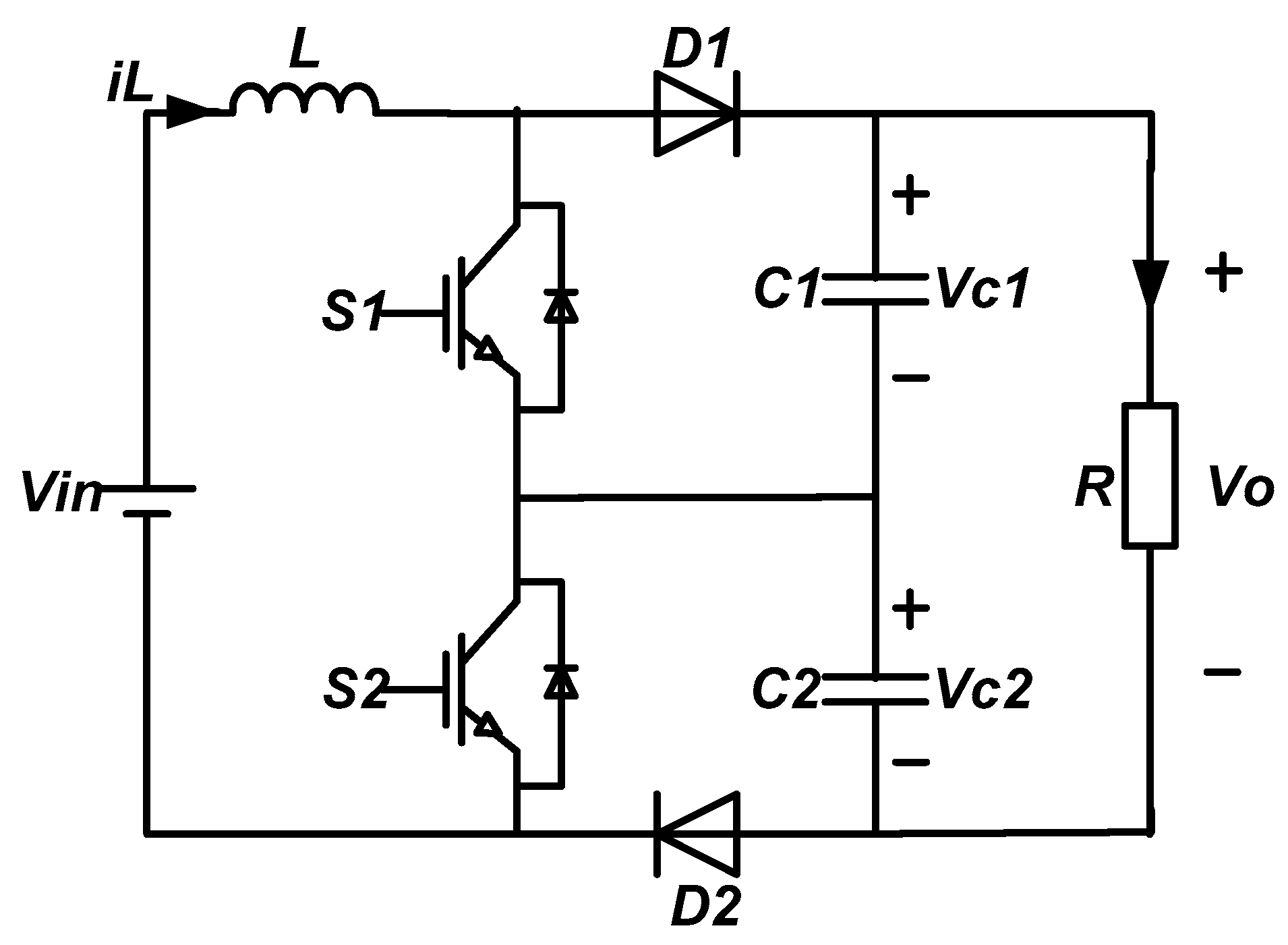
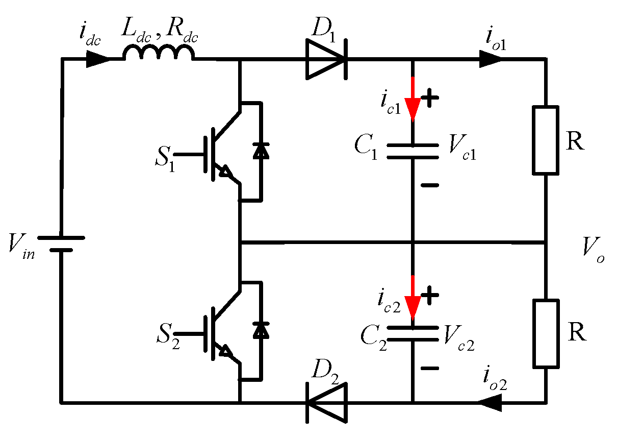
Figure 2 shows the main circuit of the boost-TL converter. and are the main power switches, L is the boost inductor, and are for the freewheeling diode, and are the voltage divider capacitors, and R is the load; and are the capacitor voltage, is the current flowing through the boost inductor, and is the output voltage.
It is assumed that the switch, the diode, the inductor, and the capacitors of the circuit are ideal components. The drive signals and have a phase difference of 180° to reduce the inductor current ripple and the output voltage ripple. = , and it is large enough to divide the supply voltage evenly, and the ratio of ripple to the output voltage is small enough to be negligible.
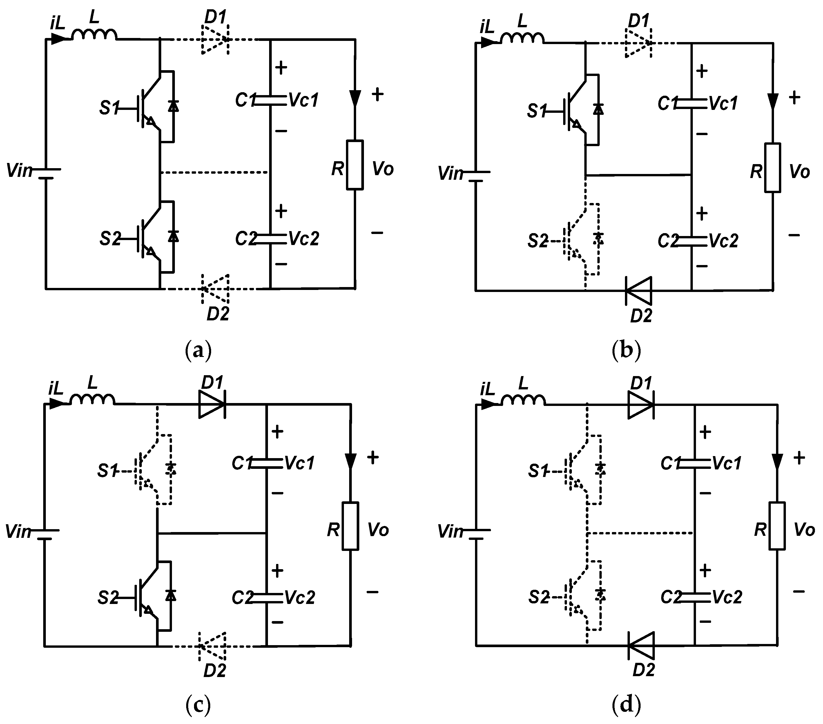
When the duty cycle of the switch is d < 0.5 or d > 0.5, the operation mode of the converter is different. The following are analyzed separately. In a switching cycle, the four operating modes of the circuit are described as follows:
- (1)
- Mode 1: switch , are on, diode , are off, inductance current increases linearly, the inductor stores energy, and the capacitors , supply energy to a load, as shown in Figure 3a.
- (2)
- Mode 2: switch is on, is off, diode is off, is on, the input voltage provides energy to the load R through a loop composed of inductor L, , and , as shown in Figure 3b.
- (3)
- Mode 3: switch is off, is on, diode is on, is off, the input voltage provides energy to the load R through a loop composed of inductor L, , and , as shown in Figure 3c.
- (4)
- Mode 4: switch is off, is off, diode is on, is on, the input voltage provides energy to the load R through a loop composed of inductor L, , and , as shown in Figure 3d.
It can be seen that when the duty cycle d < 0.5, the operating modes include modes 2, 3, and 4, and there is no mode 1; when the duty cycle d > 0.5, modes of operation include modes 1, 2, and 3, and no mode 4. When the switch duty cycle d < 0.5, according to the voltage voltage-second balance at both ends of the inductor during a switching cycle, the following results can be obtained:
From Equation (1):
When the switch duty cycle d > 0.5, for the same reason, according to the voltage voltage-second balance at both ends of the inductor during a switching cycle, the following results can be obtained:
According to the above formula, which can be introduced into the relationship between the input and output and is still satisfied by , which means when the duty cycle d > 0.5 and d < 0.5, the converters have the same input-output relationship. If the output capacitance is equally divided, the output voltage, which is , and , can be further obtained:
It can be seen from the above formula that the boost-TL converter has the same input and output voltage relationship as the traditional boost converter.
3. Principle of the T-Type Three-Level Inverter
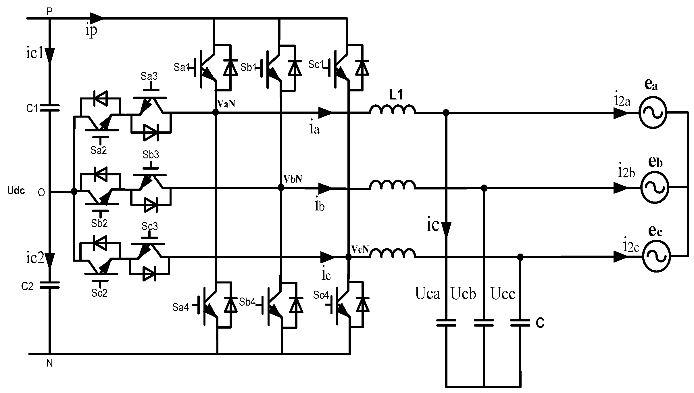
In recent years, The T-type three-level inverter has been widely used in photovoltaic (PV) inverters, power factor correction (PFC) rectifiers, automatic rectification, and other low-voltage systems [13]. Figure 4 shows a simplified circuit for a T-type inverter. T-type inverters use the same switches as conventional two-level inverters because these switches ( and ) have to block the full DC link voltage. A bidirectional switch is connected between the neutral point and each output. Unlike the half-bridge switches ( and ), the bidirectional switches ( and ) only need to block half the DC link voltage. Therefore, the devices with lower voltage ratings can be used. A neutral point clamp inverter (NPC) uses two switches connected in series to block the voltage across the DC link. On the other hand, T-type inverters use a single switch to block the voltage across the DC link. Therefore, the T-type inverter conduction loss is greatly reduced compared to that of the NPC inverter. The T-type inverter reduces switching losses and switching noise because the neutral switch operates below half the DC link voltage. Therefore, the total losses in a T-type inverter are the lowest among those of the two-level, NPC, and T-type inverters at medium switching frequencies (4–30 kHz).
Considering the switch combinations based on Table 1, this configuration allows three voltage levels related to neutral 0 to be generated at the output of phase x.
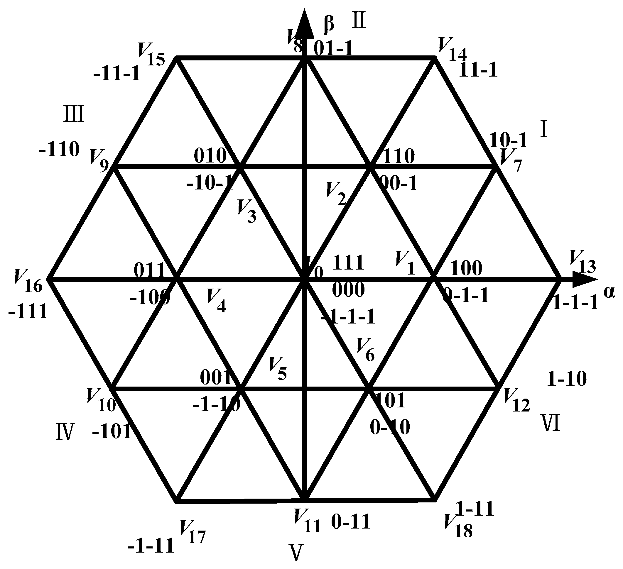
For the T-type inverter, the number of switching states is 27, including 19 different voltage vectors, as shown in Figure 5, where some switching states are redundant and generate the same voltage vector. Compared with the two-level inverter, the three-level T-type inverter shows a higher number of switching states. Greater possible incentive mechanisms allow for additional degrees of freedom, and several combinations of cost functions can be considered [14].
The general predictive control scheme is adopted in the T-type inverter [15]. The behavior of the system can be predicted for every possible switching state of this converter. We choose to minimize the switching state for a given cost function for use in the next sampling interval. Compared with the two-level inverter, the T-type inverter has a higher number of switching states. A larger set of possible drivers allows for additional degrees of freedom, and several combinations of cost functions can be considered. Considering the requirements of the control system, the characteristic and its applications of this topology are studied and compared with the classical PWM linear control algorithm, including load current reference tracking, balancing the DC link capacitor voltage, reducing the switching frequency, and so on [16]. With the development of microprocessor technology [17], the predictive control has been widely applied in power systems. Finite control set model predictive control (FCS-MPC) is more suitable for power electronic converters. The controller is intuitive and easy to implement, and can be used in a number of systems with constraints and/or non-linearly.
In this article, the control strategy is summarized as follows: 1. Define a cost function; 2. Create a transformer model and its possible switch states; and 3. Create a grid model for forecasting. A discrete time model of the load is required for the predicting behavior of the evaluated variable by a cost function, that is, the grid current.
4. Predictive Current Control Strategy
4.1. Predictive Current Control of the BTL
Comparing with the conventional boost converter, the current ripple of the inductor in the boost-TL converter is lower, which reduces the torque ripple of the generator. The voltage stress on the power unit is small, which is only the voltage stress of the common boost converter. In the same inductor current, the switching frequency is half of the common boost converter, so the switching loss is less, and the boost-TL converter can be in the low-speed. The rectifier output DC voltage boost, therefore, can also make the wind turbine operate in a very wide speed range.
There is only one switch in a two-level boost converter, so there are only 0 or 1 () conduction modes. As shown in the TLB converter, there are upper and lower arms of the two switches, therefore, the conduction of the switch tube () has four different modes, namely, (00, 01, 10, 11). The increase of the operating modes increases the number of states of switching-on of the switch, resulting in the need to increase the degree of freedom of control of charging and discharging the DC-side equalizing capacitor.
For the four operating modes in Figure 6, respectively, the Kirchhoff voltage and current formula can be linear continuous systems for the DC-side inductor current and capacitor voltage, respectively:
where , are the boost-TL circuit power switching signals; and and are the flowing currents through the load. The voltages across the capacitor at can be obtained, respectively, by:
As can be seen from the equations above, by measuring the moment of the inductor current, the two ends of the voltage divider capacitor, the load test output current, and the two switches show four possible conduction states, and the output voltage at the next moment’s predictive value can be obtained:
4.2. The Predictive Current Control Scheme of the T-Type Inverter
4.2.1. Model of Grid-Connected
Considering the definition of the circuit variables shown in Figure 4, ignoring the capacitor current flow, the dynamics equations of load current for each phase can be obtained:
where R is the load resistance and L is the load inductance.
Considering the unitary vector , which represents the 120° phase shift between the phases, the output voltage vector can be defined as:
4.2.2. Discrete-Time Model of Prediction
The discrete-time model is used to predict the future value of the grid current at the kth instant sampling the instantaneous voltage and measured current [18]. Several discrete methods are used in order to obtain a suitable predictive computing discrete-time model.
Use the forward Euler approximation to replace the grid current derivative . That is, the derivatives are approximated as follows:
This is substituted into Equation (9) to obtain an equation that allows the prediction of the future load currents at time for each of the 27 voltage vectors generated by the inverter. This equation is:
where represents the estimated back EMF. The superscript p indicates the predictor.
The reference currents can be calculated by considering the active and reactive power reference , . According to instantaneous power theory [19], the system instantaneous active power and reactive power can be calculated using the following expressions:
Thus, it is easy to obtain the reference current:
Back-EMF voltage can be calculated from Equation (10). Considering the measurement of the load voltage and current, the equation is as follows:
where is the estimated value of . The present back-EMF is , the value of the back-EMF can be estimated by extrapolating it, or, since the back-EMF frequency is much less than the sampling frequency, we can assume that within a sampling interval little change happens. Therefore, assume . The same derivative approximation can be used for the capacitor voltage at sampling time which gives the following discrete-time equation:
where, the currents and depend on the switching state of the T-type inverter and the values of the output currents can be calculated from the following equations:
where is the current supplied by the DC voltage source . Variables and depend on the logical value of the switching states and are defined as:
with .
Therefore, Equations (13)–(16) predict the influence of a given switch state on the change of capacitor voltage [20].
4.2.3. Predictive Current Control Method
The T-type inverter control requirements are as follows:
- A reference for grid current tracking;
- DC link capacitor voltage neutral point balancing;
- Reducing the switching frequency.
These requirements can be expressed in the form of a cost function so that the cost function can be minimized. The T-type inverter has the following components:
The first two terms are the load current errors in orthogonal coordinates in which the real part and the imaginary part of the predicted current vector are and , respectively, and the real part and the imaginary part of the reference current vector are and , respectively. The third cost function measures the difference between the capacitors’ voltages of the predicted DC link, which are calculated from Equations (19) and (20). Then, by minimizing this term, the voltages of the capacitors will tend to be equal. The last item is the number of transitions needed to switch from the current switch state to the switch state being evaluated. Switching states mean fewer switching power semiconductors, which is preferred.
In this way, the use of these terms will directly affect the switching frequency of the converter [21]. The relationship between the weighting factors and is used for reference tracking, the voltage balance, and the cost function in the reduction of the switching frequency.
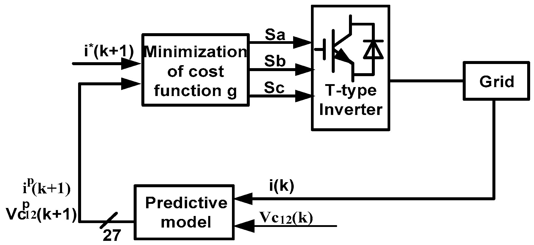
Certain values mean higher priorities to that objective. The predictive current control method for the T-type inverter is shown in Figure 7.
4.3. Cost Function Selection
4.3.1. The Optimization of the MPCC
Minimization of the switching frequency. As with power converters, one of the primary measures of control effectiveness is the switching frequency. In many applications, it is important to control or limit the commutations number of the power switches [22]. To consider directly the reduction in the number of exchanges in the cost function, a simple method is to include a term that covers the number of switches that change when the switching state is applied relative to the switching state of the previous application. The resulting cost function is expressed as . Taking the three-phase inverter as an example, the switching state vector , the switching state of each inverter arm [23] is defined. Then the number of switches changes from time to time is:
The optimization of the MPCC. In order to ensure the control accuracy of the system, the calculation speed of each sampling period must be improved, and the calculation amount in each period should be reduced.
In this paper, we introduce a method that can reduce the computational cost by simplifying the optimal switching state selection method, while ensuring that the performance of the T-type three-level grid-connected system will not be affected in any way. From the Kirchhoff’s voltage formula, we can obtain Equation (28):
If the predicted current reference value at is, instead of the actual sampling current prediction value, at the time, the corresponding voltage vector is directly tracked by using the current , i.e.:
If the voltage vector at the time corresponding to the switching state is consistent with the predicted voltage value of the next cycle, it is indicated that the current sampling at the same time is consistent with the reference current value . Therefore, as long as the switching state closest to the predicted voltage value is selected among the voltage vectors corresponding to the 27 switching states to drive the switch at the next moment, the grid-connected current can be tracked. That is, as Equation (30) shows:
In that formula, represent, respectively, the real part and the imaginary part of the voltage vector in the coordinate system.
4.3.2. Cost Function of the Capacitor Voltage Balance
One of the most interesting aspects of predictive control methods is the simplicity of voltage balance in the DC bus [24]. This feature disconnects the midpoint of the DC bus from the source and combines the predictive control method with the following cost function:
In this control method, it is necessary to adjust the parameters and . To this end, some design procedures of the system should be established. The different units and sizes of the variables involved in the cost function should be considered [25]. Some ideas will be given, which, from the order of magnitude of the weighting factors, are of equal importance. If the designer just wants to select the appropriate switch state from the redundancy state that produces the given voltage vector to maintain neutral point voltage balance in the DC link, a small value of should be adopted. The minimum value allowed by the platform will work for this purpose. The same principle has been applied to . When increasing , this method can select the switching state in the reference tracking that does not belong to the optimal voltage vector range, but this means fewer commutations.
On this basis, the method of predictive current control is realized, and the simulation results are verified. This strategy successfully maintains the voltage balance of the DC link and reduces the switching frequency. Compared with the carrier-based approach, this method achieves better reference tracking at the same switching frequency.
4.3.3. The Cost Function of the Predictive Control Scheme
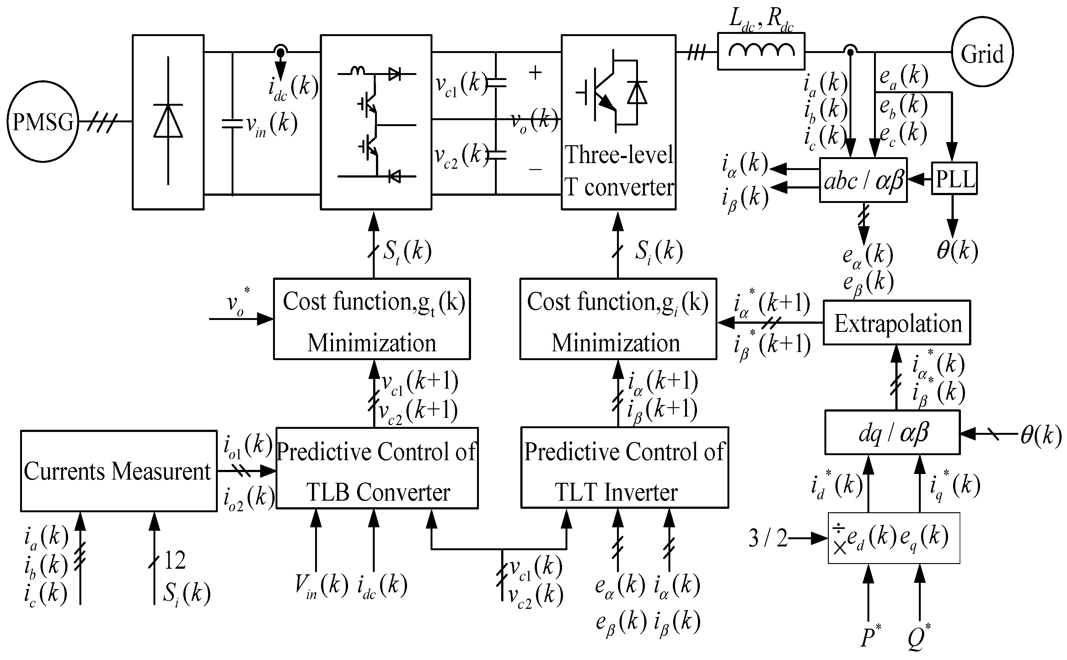
Control of the pre-output voltage stability is to ensure that the entire system is running the primary task. In this paper, the post-stage T-type three-level inverter is used to balance the midpoint potential of the first-stage three-level boost DC side, and the modulation algorithm of the grid-side three-level converter on the redundant small vector is refined. The predictive control scheme of the BTL and three level T-type inverter is shown in Figure 8.
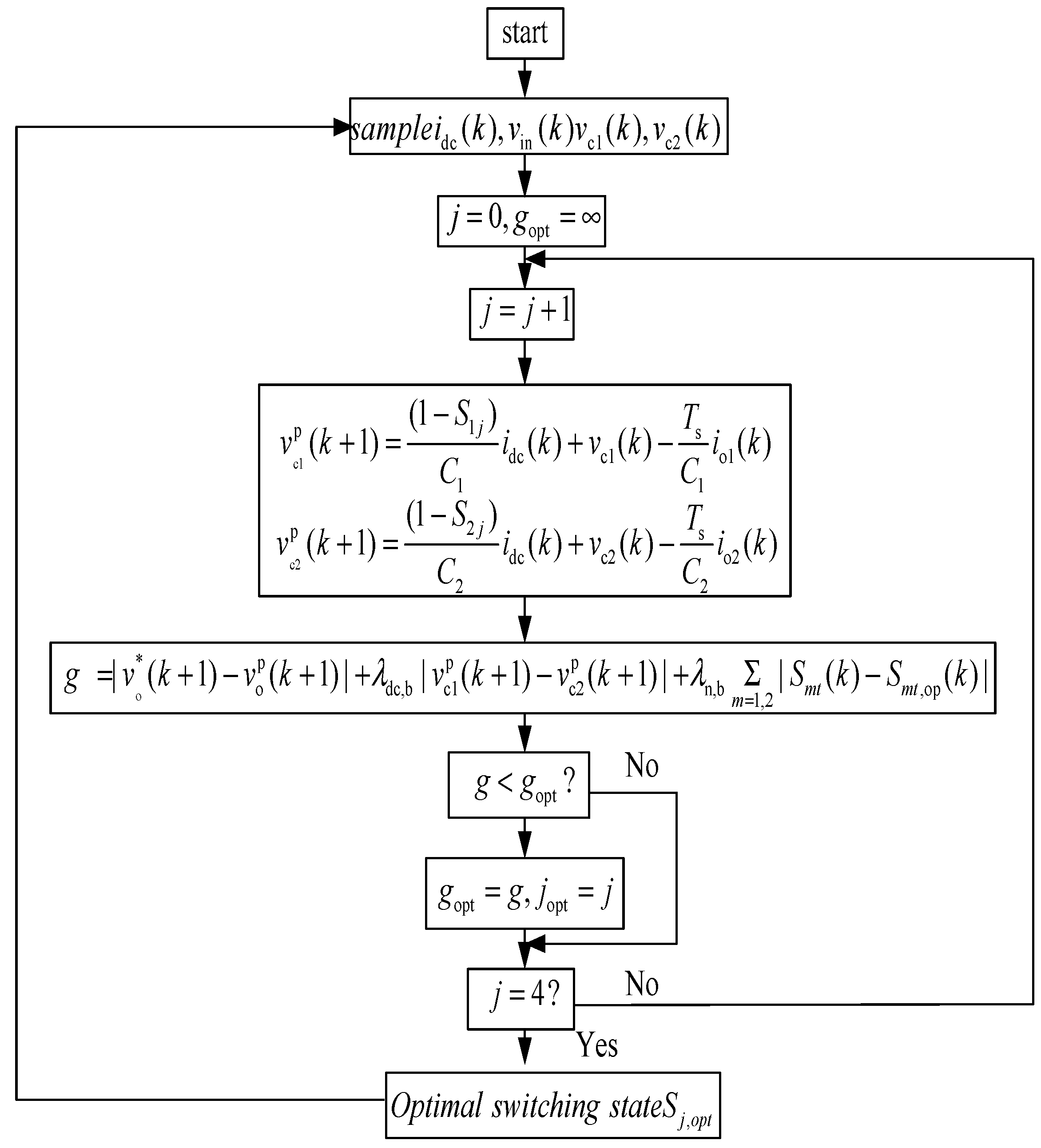
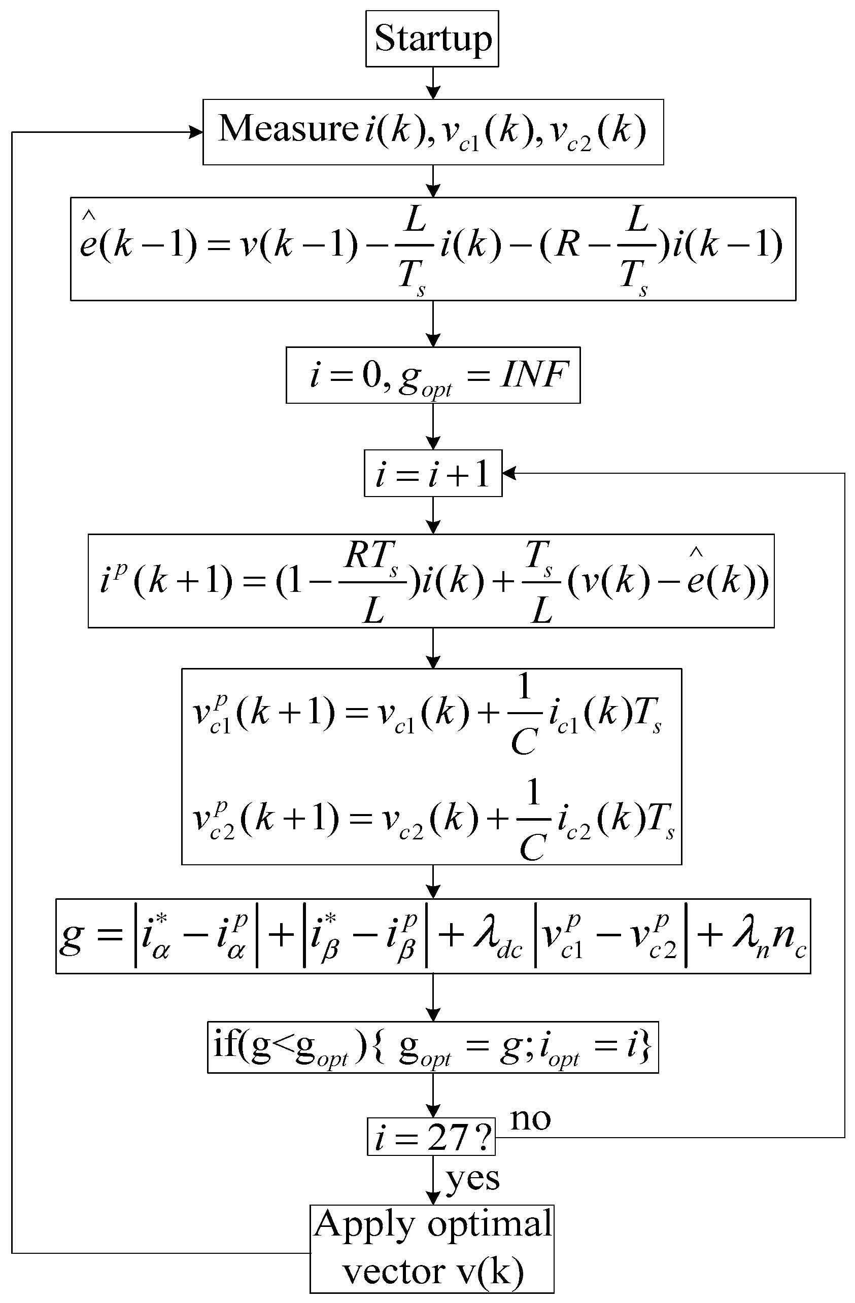
Regarding the three-level T-inverter model predictive control mentioned earlier, the FCS-MPC predictive control algorithm of the cascade structure is the difference from the previous output current, which was obtained by measuring the three-level inverter output current. The cost function flow chart of the boost-TL converter model prediction algorithm and the T-type inverter model prediction control algorithm are shown in Figure 9 and Figure 10, respectively.
The closed-loop requirement is robust stability, i.e., stability in the presence of uncertainty. In MPC the various design procedures achieve robust stability indirectly by specifying the performance objective and uncertainty description in such a way that the optimal control computations lead to robust stability.
5. Simulations and Experimental
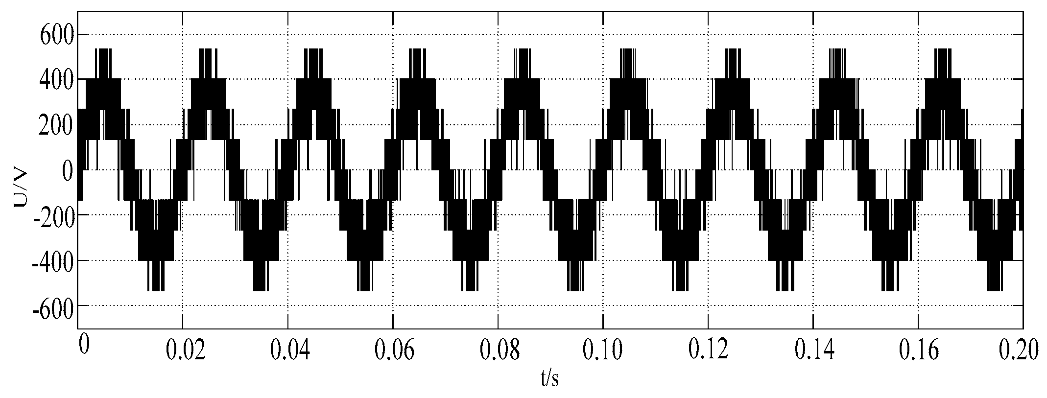
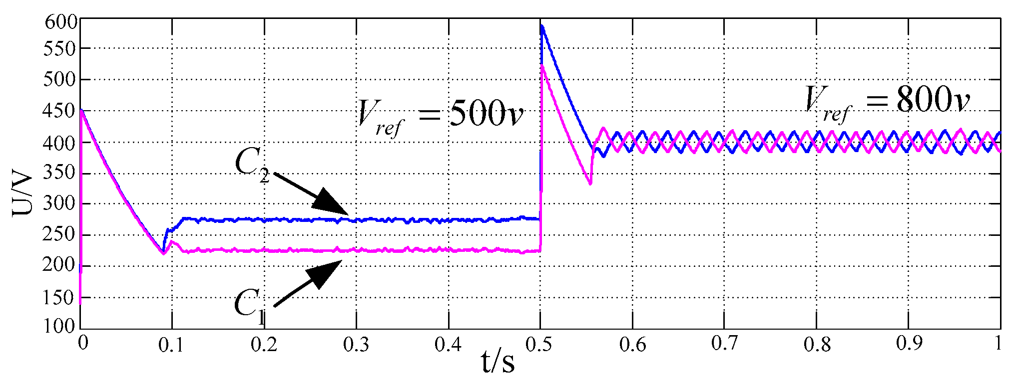
The control strategy of the predictive current is simulated in MATLAB(R2013), containing the code of the control algorithm, as shown in Figure 8. When experimentally implementing predictive control, the same procedure was rewritten in the C language and the alpha and beta currents were calculated. In the MATLAB/SIMULINK environment, the load current prediction (Equation (14)) and back EMF estimation (Equation (17)) are considered. The system parameters , , , and have been taken into account for the simulations. The current and voltage in one of the phases of the load are simulated for a sampling time . There is no steady state error from the current, but there is an obvious ripple. The ripple is significantly reduced when the smaller sampling time is adopted. However, by reducing the sampling time, the switching frequency increases, as shown in the load voltage comparison shown in Figure 13. The inverter output phase voltage is shown in Figure 11. When the reference voltage value rises from 500 V to 800 V, the change of the capacitance voltage is shown in Figure 12.
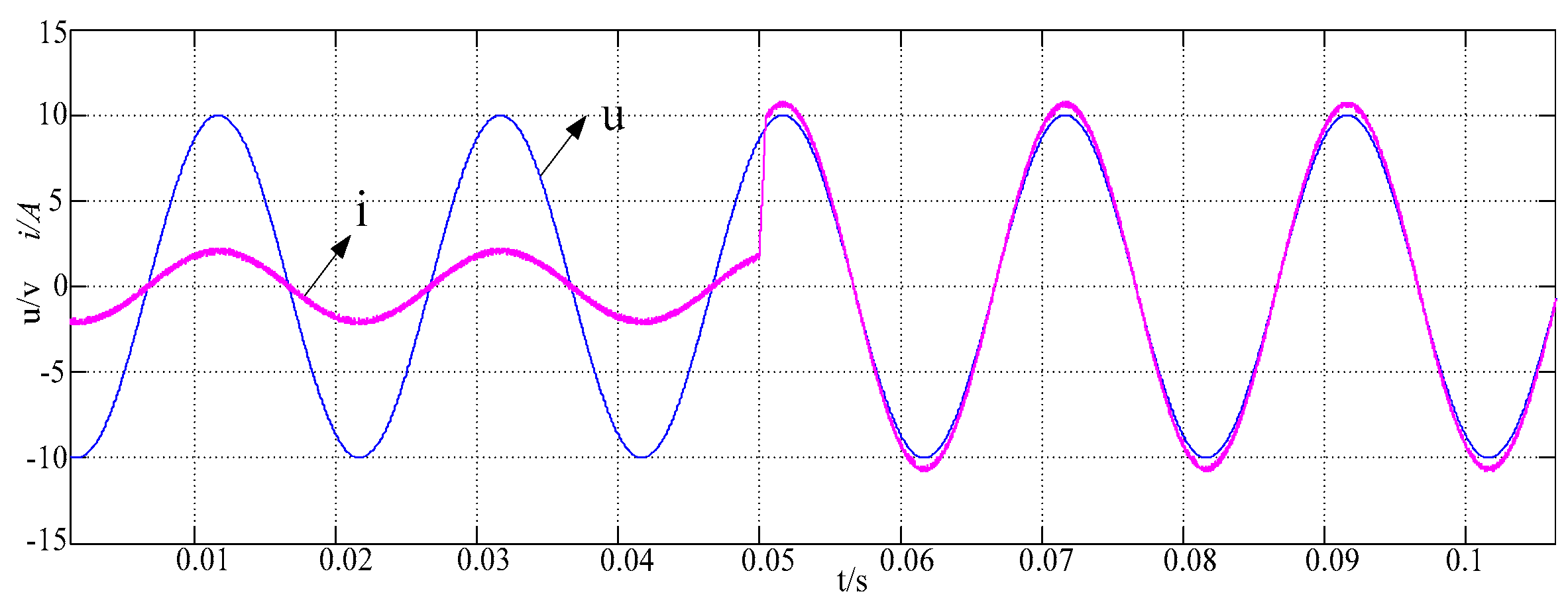
As shown in Figure 13, the value of the reference power is changed at , and the corresponding reference current phase can still stably track the grid voltage phase, and the response speed is fast.
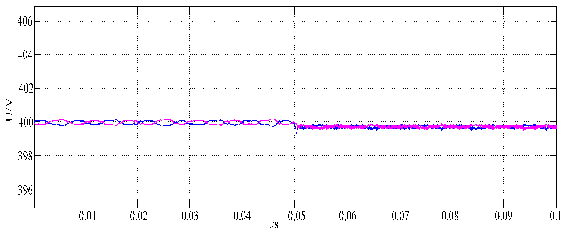
With the change of the reference current, the voltage of the divider capacitor becomes more and more stable when the weight factor increases, and the two are close to equal, as shown in Figure 14.
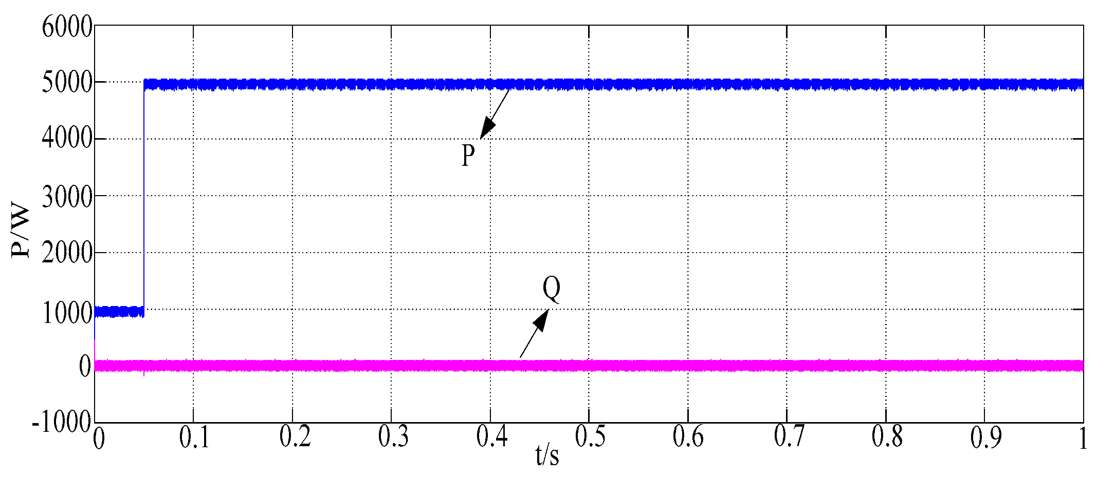
When changing the value of the reference power, the system can respond quickly. As shown in Figure 15.
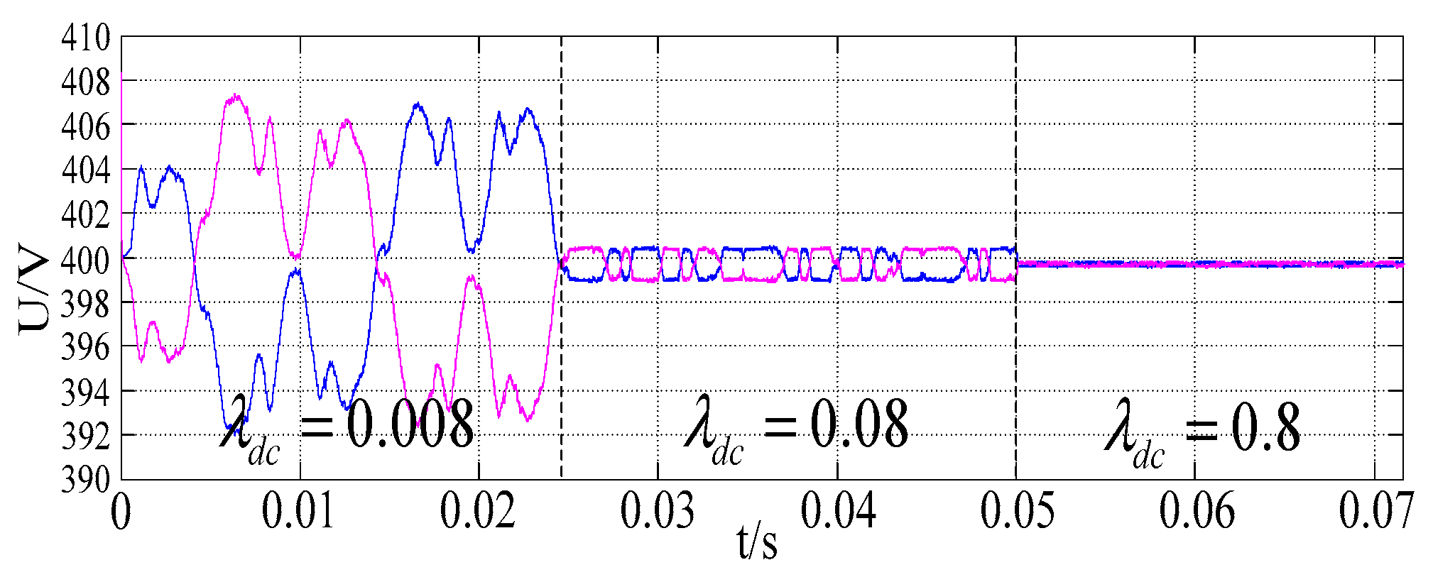
At the same time, the control level of the voltage-dividing capacitance increases with the increase of the weighting factor when observing the increase of the magnitude of the weight factor of the division of the voltage-dividing capacitance, which is the same as the conclusion, as shown in Figure 16.
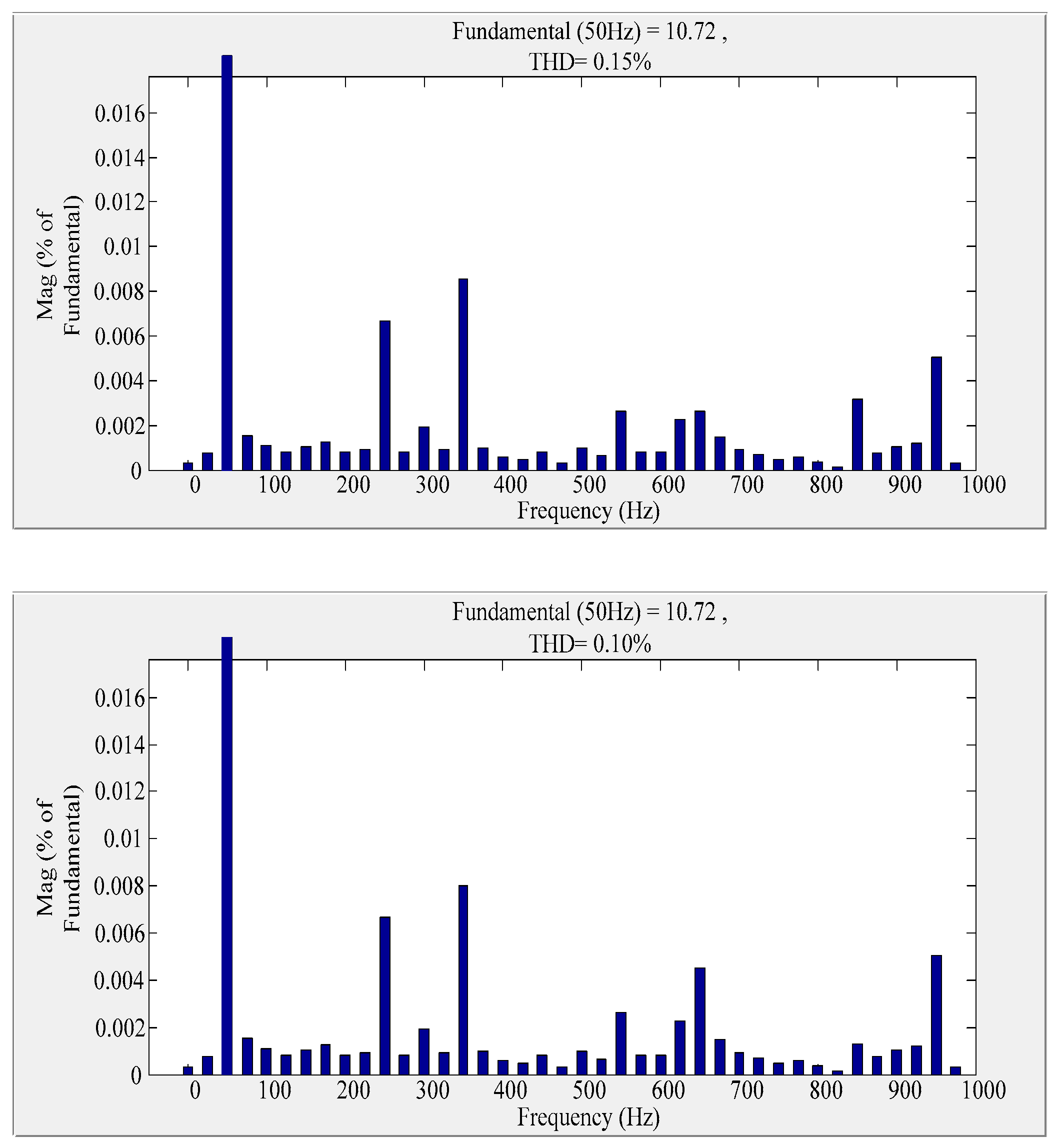
As shown in Figure 17, it is obvious to say that the rise of the weighting factor of the current tracking can optimize the THD from 0.15% to 0.10%.
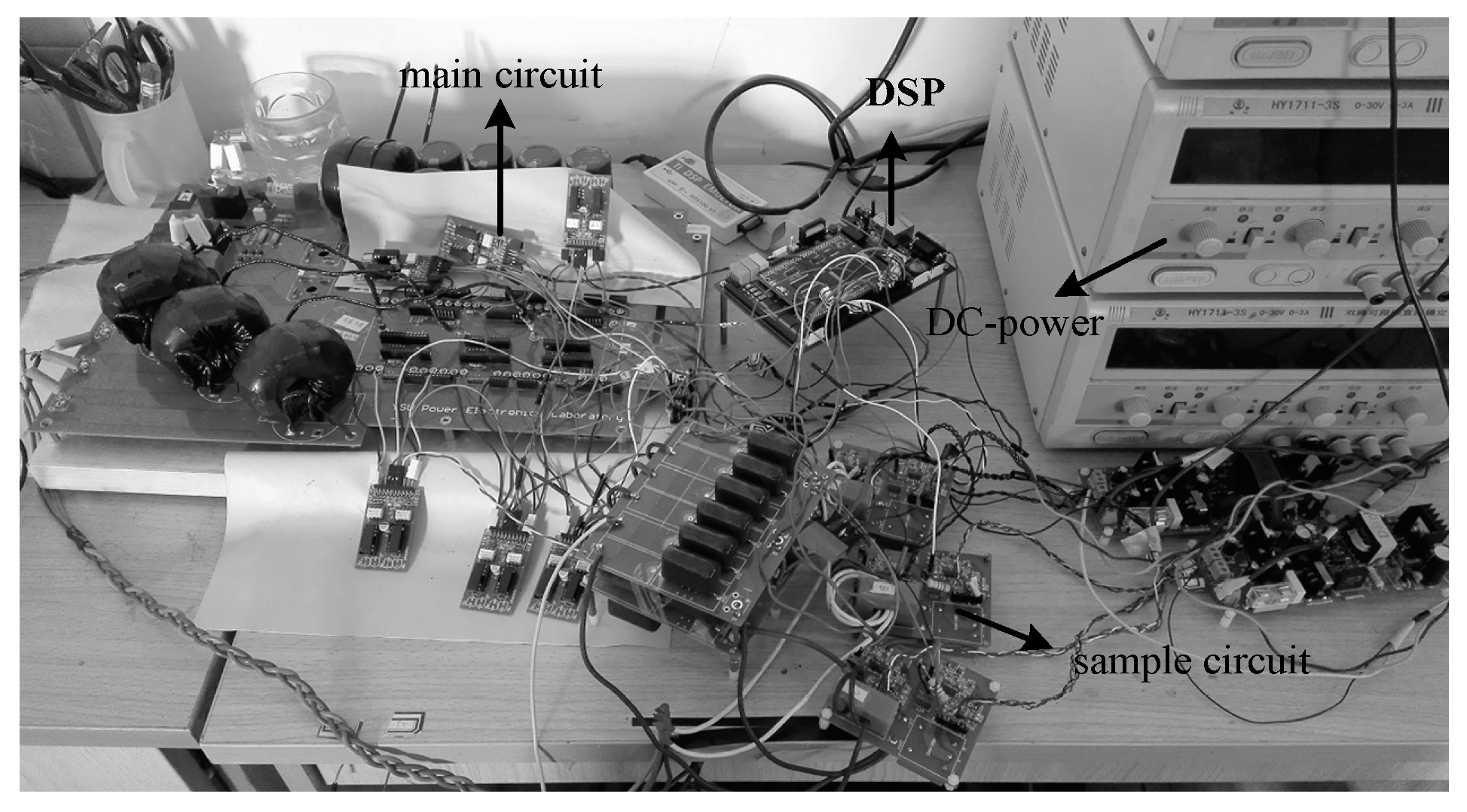
The proposed control method requires a higher sampling or data acquisition frequency. Given the new technologies available for DSP, the foregoing fact should not be a problem. It is worth mentioning that the sampling time is always a fixed position in the sampling period, to facilitate the acquisition of measurement data and to avoid the problem of the switching the power devices. The algorithm is implemented on a Texas Instruments DSP using the same sampling frequency. The algorithm was implemented on the Texas Instruments TMS320F2812 DSP using the same sampling frequency, and similar results in processing time were achieved. The experimental platform is shown in Figure 18 to determine whether the driving circuit can work normally, which plays a key role in the whole system’s working state. First, according to the working principle of the driving circuit analyzed above, we designed and built the corresponding driving module. The drive signal is shown in Figure 19.
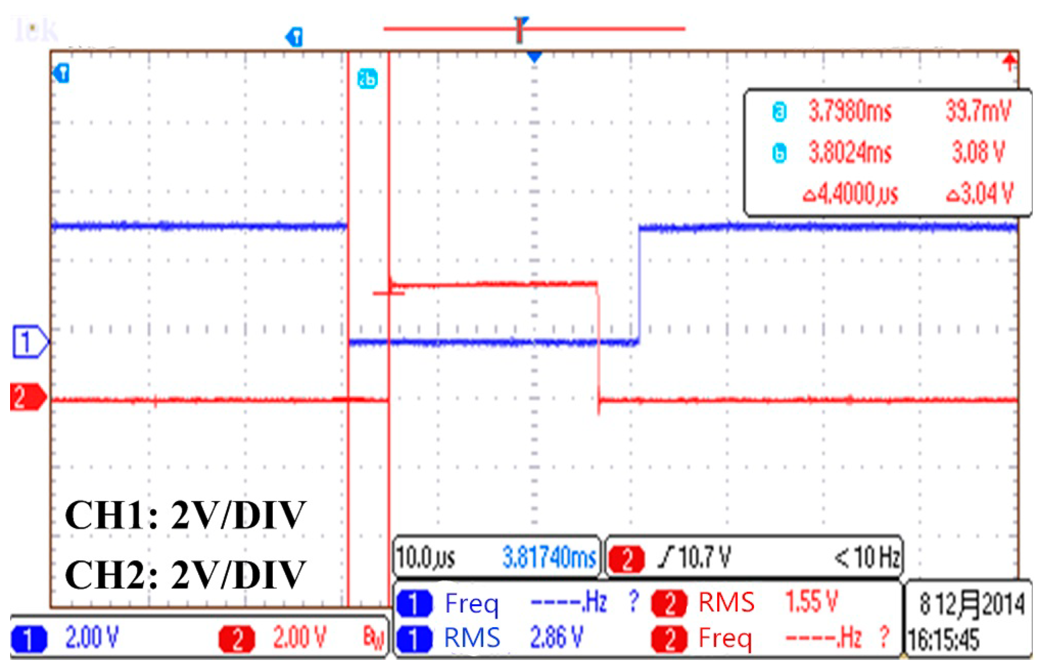
The waveforms in the same bridge arm are supposed to be complementary to each other. In order to avoid the two tubes in the same bridge arm conducting at the same time, dead time is added in the driving signal between , and , as shown in Figure 20.
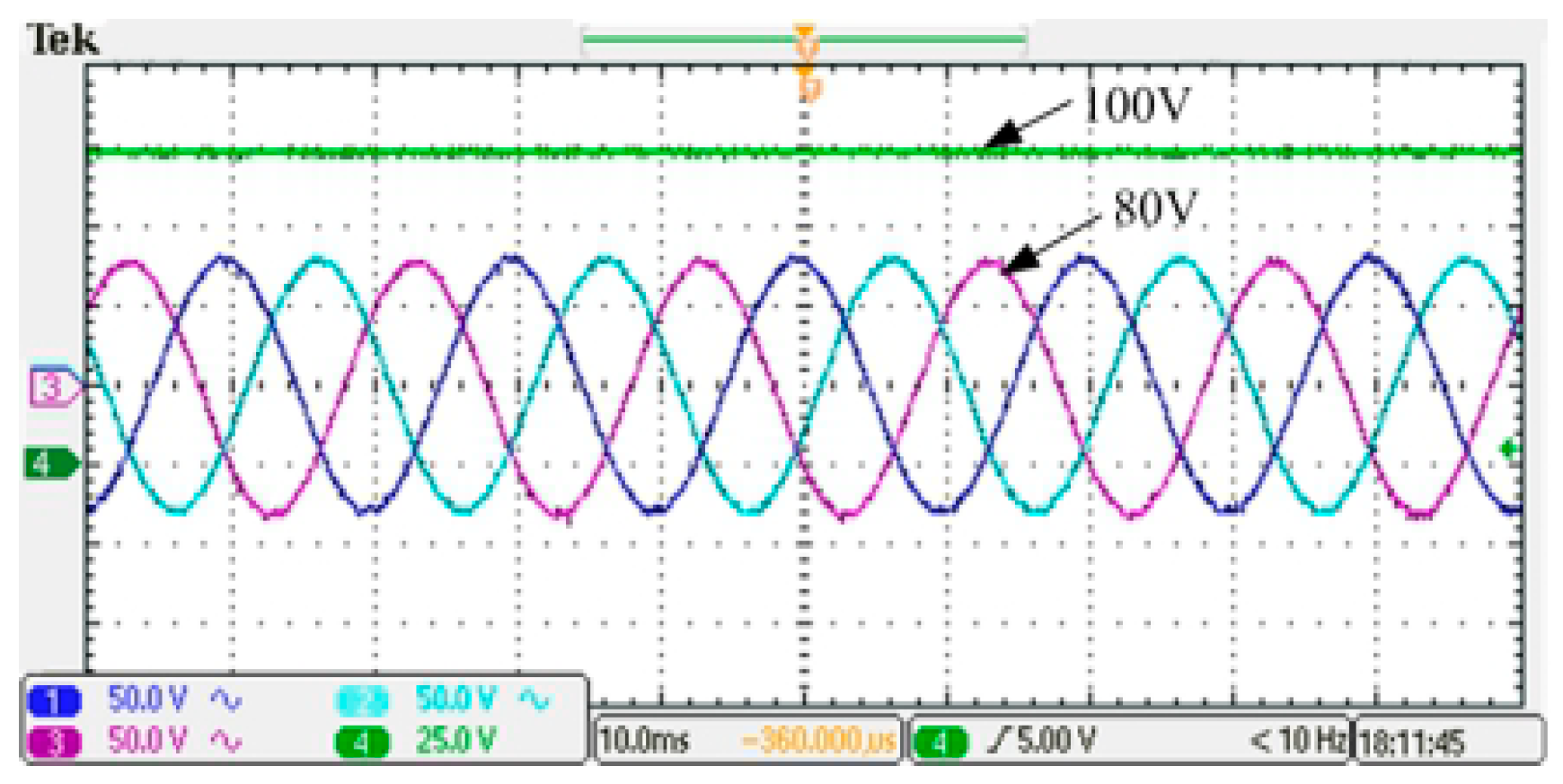
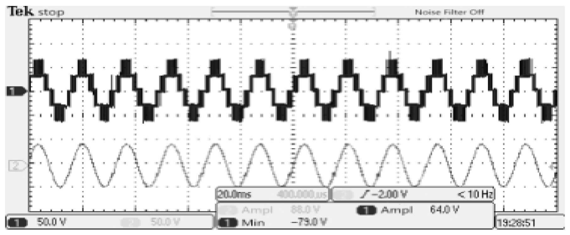
As shown in Figure 21, the input DC voltage is 50 V. Adjusting the duty cycle, the DC bus voltage is increased to 100 V, and the inverter output voltage at this time is 80 V. In order to ensure the safety of experimental operation, the voltage amplitude of AC voltage regulator is also transferred to 80 V, the grid connection is realized after synchronization control.
The waveforms of the output line voltage and current are shown in Figure 22. All of these experimental waveforms demonstrate the correctness and effectiveness of the proposed control scheme.
6. Conclusions
This paper proposed that the boost three-level circuit (BTL) and the three-level T-type inverter are cascaded together and controlled in a unified manner in a wind power system. By controlling the voltage balance between the two capacitors at the connection between the two stages, the output voltage is stable. The predictive control scheme is designed by adopting the model predictive current control method. By adjusting the weight factor parameter to balance the neutral point voltage in the DC link, the switching frequency and THD were reduced, the parameter tracking and fast response were realized. The model predictive current control algorithm has been optimized, and the calculation amount of the optimized algorithm in each period has been reduced. The disadvantage of this method is the need for delay compensation. The simulation and experimental verification show that the proposed structure and control methods are correct and feasible.
Author Contributions
G.Y. and Z.C. proposed the topology of the system; H.Y. and B.H. devoted to performing the simulations; G.Y., C.C. and Y.Z. conducted the experiments; and G.Y. wrote the paper.
Funding
This paper is supported by the Science and Technology project of Hebei province, China, under grant no. 15214318, and the University research program of Xinjiang Uygur Autonomous Region, China, under grant no. XJEDU2016S114.
Conflicts of Interest
The authors declare no conflict of interest.
References
- Carrasco, J.; Franquelo, L.; Bialasiewicz, J.; Galvan, E.; Guisado, R.; Prats, M.; Leon, J.; Moreno-Alfonso, N. Power-electronic systems for the grid integration of renewable energy sources: A survey. IEEE Trans. Ind. Electron. 2006, 53, 1002–1016. [Google Scholar] [CrossRef]
- Kolar, J.W.; Friedli, T.; Rodriguez, J.; Wheeler, P.W. Review of Three-Phase PWM AC-AC Converter Topologies. IEEE Trans. Ind. Electron. 2011, 58, 4988–5006. [Google Scholar] [CrossRef]
- Chen, H.-C.; Lin, W.-J. MPPT and Voltage Balancing Control with Sensing Only Inductor Current for Photo Voltaic-Fed, Three-Level, Boost-Type Converters. IEEE Trans. Power Electron. 2014, 29, 29–35. [Google Scholar] [CrossRef]
- Liang, X.; Zhang, C.; Srdic, S.; Lukic, S. Predictive Control of a Series-Interleaved Multi-Cell Three-Level Boost Power Factor Correction Converter. IEEE Trans. Power Electron. 2017. [Google Scholar] [CrossRef]
- Kouro, S.; Cortés, P.; Vargas, R.; Ammann, U.; Rodriguez, J. Model predictive control a simple and powerful method to control power converters. IEEE Trans. Ind. Electron. 2009, 56, 1826–1838. [Google Scholar] [CrossRef]
- Yaramasu, V.; Wu, B. Predictive control of a three-level boost converter and an NPC inverter for high-power pmsg-based medium voltage wind energy conversion systems. IEEE Trans. Ind. Electron. 2014, 29, 5308–5322. [Google Scholar] [CrossRef]
- Baggio, J.; Hey, H.; Grundling, H.; Pinheiro, H.; Pinheiro, J. Discrete control for three-level boost PFC converter. In Proceedings of the 24th Annual International Telecommunications Energy Conference, Montreal, QC, Canada, 29 September–3 October 2002; pp. 627–633. [Google Scholar]
- Xing, X.; Chen, A.; Zhang, Z.; Chen, J.; Zhang, C. Model Predictive Control Method to Reduce Common-Mode Voltage and Balance the Neutralpoint Voltage in Three-Level T-type Inverter. In Proceedings of the 2016 IEEE Applied Power Electronics Conference and Exposition (APEC), Long Beach, CA, USA, 20–24 March 2016; pp. 3453–3458. [Google Scholar]
- Abdel-Rahim, O.; Takeuchi, M.; Funato, H.; Junnosuke, H. T-type three-level neutral point clamped inverter with model predictive control for grid connected photovoltaic applications. In Proceedings of the 2016 19th International Conference on Electrical Machines and Systems (ICEMS), Chiba, Japan, 13–16 November 2016; pp. 1–5. [Google Scholar]
- Han, B.; Kong, X.; Zhang, Z.; Zhou, L. Neural network model predictive control optimisation for large wind turbines. IET Gener. Transm. Distrib. 2017, 11, 3491–3498. [Google Scholar] [CrossRef]
- Wang, X.; Sun, D. Three-Vector-Based Low-Complexity Model Predictive Direct Power Control Strategy for Doubly Fed Induction Generators. IEEE Trans. Ind. Electron. 2017, 32, 773–782. [Google Scholar] [CrossRef]
- Bayhan, S.; Abu-Rub, H.; Ellabban, O. Sensorless model predictive control scheme of wind-driven doubly fed induction generator in dc microgrid. IET Renew. Power Gener. 2016, 10, 514–521. [Google Scholar] [CrossRef]
- Nabae, A.; Takahashi, I.; Akagi, H. A new neutral-point-clamped PWM inverter. IEEE Trans. Ind. Appl. 1981, IA-17, 518–523. [Google Scholar] [CrossRef]
- Wu, B. High-power converters and AC motor drives. In Proceedings of the Power Electronics Specialists Conference, PESC’05, Recife, Brazil, 12–16 June 2005. [Google Scholar]
- Jana, K.C.; Biswas, S.K. Generalised switching scheme for a space vector pulse-width modulation-based N -level inverter with reduced switching frequency and harmonics. IET Power Electron. 2015, 8, 2377–2385. [Google Scholar] [CrossRef]
- Latran, M.B.; Teke, A. Investigation of multilevel multifunctional grid connected inverter topologies and control strategies used in photovoltaic systems. Renew. Sustain. Energy Rev. 2015, 42, 361–376. [Google Scholar] [CrossRef]
- Cui, B. T-Type Three-Level Inverter Circuit. U.S. Patent US8665619B2, 4 March 2014. [Google Scholar]
- Cortes, P.; Rodriguez, J.; Silva, C.; Flores, A. Delay Compensation in Model Predictive Current Control of a Three-Phase Inverter. IEEE Trans. Ind. Electron. 2012, 59, 1323–1325. [Google Scholar] [CrossRef]
- Holtz, J. Pulsewidth modulation for electronic power conversion. Proc. IEEE 1994, 82, 1194–1214. [Google Scholar] [CrossRef]
- Duran, M.J.; Prieto, J.; Barrero, F.; Toral, S. Predictive current control of dual three-phase drives using restrained search techniques. IEEE Trans. Ind. Electron. 2011, 58, 3253–3263. [Google Scholar] [CrossRef]
- Vargas, R.; Rodriguez, J.; Ammann, U.; Wheeler, P.W. Predictive current control of an induction machine fed by a matrix converter with reactive power control. IEEE Trans. Ind. Electron. 2008, 55, 4362–4371. [Google Scholar] [CrossRef]
- Cortes, P.; Rodriguez, J.; Quevedo, D.E.; Silva, C. Predictive current control strategy with imposed load current spectrum. IEEE Trans. Power Electron. 2008, 23, 612–618. [Google Scholar] [CrossRef]
- Rodriguez, J.; Cortes, P. Predictive Control of Power Converters and Electrical Drives; John Wiley & Sons Ltd.: Chichester, West Sussex, UK, 2012. [Google Scholar]
- Xia, C.; Liu, T.; Shi, T.; Song, Z. A Simplified Finite Control Set Model Predictive Control for Power Converters. IEEE Trans. Ind. Inform. 2013, 28, 1–12. [Google Scholar]
- Cortes, P.; Wilson, A.; Kouro, S.; Rodriguez, J.; Abu-Rub, H. Model Predictive Control of Multilevel Cascaded H-Bridge Inverters. IEEE Trans. Ind. Electron. 2010, 57, 2691–2699. [Google Scholar] [CrossRef]
Figure 1.
BTL and T-type three-level inverter.

Figure 2.
Main circuit of the boost-TL converter.

Figure 3.
Four operating modes of boost-TL converters.

Figure 4.
T-type inverter.

Figure 5.
Voltage vectors and switching states of the T-type inverter.

Figure 6.
The main boost-TL circuit.

Figure 7.
T-type inverter predictive current control method.

Figure 8.
Predictive control scheme of the BTL and the three-level T-type inverter.

Figure 9.
The cost function flow chart of the boost-TL converter model prediction algorithm.

Figure 10.
The cost function flow chart of the T-type inverter model prediction control algorithm.

Figure 11.
Output voltage of phase A.

Figure 12.
Change in the reference voltage value.

Figure 13.
The voltage phase and current phase are consistent.

Figure 14.
Capacitor voltage of C1 and C2.

Figure 15.
Power tracking.

Figure 16.
The influence of adjusting the weight factor of the capacitor voltage.

Figure 17.
The influence of adjusting the weight factor of the capacitor voltage.

Figure 18.
Experimental platform.

Figure 19.
Drive signal.

Figure 20.
Dead time.

Figure 21.
DC voltage waveform and inverter side filter voltage waveform.

Figure 22.
Output line voltage and current waveform.


Table 1.
Switching states in one phase of the inverter.
| Sx1 | Sx2 | Sx3 | Sx4 | Sx | Uout |
|---|---|---|---|---|---|
| on | on | off | off | P | |
| 0 | on | on | off | 0 | 0 |
| off | off | on | on | N |
© 2018 by the authors. Licensee MDPI, Basel, Switzerland. This article is an open access article distributed under the terms and conditions of the Creative Commons Attribution (CC BY) license (http://creativecommons.org/licenses/by/4.0/).
Share and Cite
MDPI and ACS Style
Yang, G.; Yi, H.; Chai, C.; Huang, B.; Zhang, Y.; Chen, Z. Predictive Current Control of Boost Three-Level and T-Type Inverters Cascaded in Wind Power Generation Systems. Algorithms 2018, 11, 92. https://doi.org/10.3390/a11070092
AMA Style
Yang G, Yi H, Chai C, Huang B, Zhang Y, Chen Z. Predictive Current Control of Boost Three-Level and T-Type Inverters Cascaded in Wind Power Generation Systems. Algorithms. 2018; 11(7):92. https://doi.org/10.3390/a11070092
Chicago/Turabian StyleYang, Guoliang, Haitao Yi, Chunhua Chai, Bingxu Huang, Yuna Zhang, and Zhe Chen. 2018. "Predictive Current Control of Boost Three-Level and T-Type Inverters Cascaded in Wind Power Generation Systems" Algorithms 11, no. 7: 92. https://doi.org/10.3390/a11070092
Note that from the first issue of 2016, this journal uses article numbers instead of page numbers. See further details here.