Computing Persistent Homology of Directed Flag Complexes

Abstract

We present a new computing package Flagser, designed to construct the directed flag complex of a finite directed graph, and compute persistent homology for flexibly defined filtrations on the graph and the resulting complex. The persistent homology computation part of Flagser is based on the program Ripser by U. Bauer, but is optimised specifically for large computations. The construction of the directed flag complex is done in a way that allows easy parallelisation by arbitrarily many cores. Flagser also has the option of working with undirected graphs. For homology computations Flagser has an approximate option, which shortens compute time with remarkable accuracy. We demonstrate the power of Flagser by applying it to the construction of the directed flag complex of digital reconstructions of brain microcircuitry by the Blue Brain Project and several other examples. In some instances we perform computation of homology. For a more complete performance analysis, we also apply Flagser to some other data collections. In all cases the hardware used in the computation, the use of memory and the compute time are recorded.

1. Introduction

In an ongoing collaboration with the Blue Brain Project [1] and the Laboratory for Topology and Neuroscience [2], we study certain ordered simplicial complexes (Definition 3) arising from directed graphs that model brain microcircuitry reconstructions created by the Blue Brain Project team. These complexes, which we refer to as directed flag complexes, generalise the usual concept of the flag complex (clique complex) associated to a graph, and prove particularly useful in studying directed networks in general and neural networks in particular.

Over the past decade, homology and persistent homology, particularly in the form of persistent homology of Vietoris–Rips complexes of point clouds, entered the field of data analysis. Therefore, its efficient computation is of great interest, which led to several computational tools like Gudhi [3], PHAT [4] and quite a number of other packages. However, working with networks, and specifically with neural networks at this order of magnitude and level of detail, presents certain challenges that can not be addressed by existing software.

One immediate problem is that network data is typically given in the form of a graph, rather than a point cloud. For instance, data emerging from the Blue Brain Project is typically encoded as a weighted directed graph. Since neurons and synaptic connections between them are modelled with great precision, if one wishes to exploit the full potential in the data, then considering the direction and weight of connections between nodes (neurons) is natural and in fact essential. To date we are not aware of any highly efficient software packages that are designed to work with directed graphs. The very impressive Gudhi package, for instance, is designed to work with simplicial complexes. The directed flag complex and numerous other topological constructions one may associate with a directed graph are not simplicial complexes. Hence to deal with networks that are directed by nature, one would need software capable of efficiently constructing various complexes one can associate with a directed graph. Furthermore, since the direction of connection does play an important role in the analysis, such software should be capable of incorporating information about direction as part of the data to be processed, beyond the mere construction of the complex.

A second issue arises from the size of the networks in question. In our earlier work we considered networks in the order of magnitude of thirty thousand vertices and eight million directed edges (reconstructed neocortical column of a 14 day old rat [5]). Software was designed as part of the work that lead to the publication [6], and is freely available [7]. However, at that time the magnitude of the resulting complexes, typically six-dimensional with about 160 million simplices across all dimensions, limited our ability to conduct certain deeper investigations, as even the construction of the complexes required a considerable number of compute hours on a large High Performance Computing (HPC) node, and homology computations with the full complex were completely out of reach. More recent reconstructions by the Blue Brain Project team produced much larger and more complex models (see for instance the model of the full mouse cortex [8]). While advanced computational packages such as Gudhi and PHAT are perfectly capable of dealing with very large simplicial complexes due to the reduction techniques they use, they too fail to produce satisfactory results on networks of the size we are interested in, within reasonable compute time.

Finally, we required a package that will allow us to flexibly associate weights to simplices in our complexes so that we could examine data with respect to a variety of filtrations. Inspired by our main object of study, neural networks, we had to take into account the fact that neurons have a very rich structure, as do connections between them. Hence associating weights to vertices and edges in the representing graph, and furthermore, using those values to induce meaningful weights on higher dimensional simplices typically involves non-obvious choices and implementations that are not catered for in existing software packages.

In this article we present a new software package, Flagser, that was developed as part of the project Topological Analysis of Neural Systems, funded by the UK’s Engineering and Physical Sciences Research Council. Flagser and its derivatives (see [9]) address the issues listed above, and show remarkable performance in many relevant cases. While Flagser is designed specifically for dealing with the kind of constructions and high performance computations required in this project, it is potentially applicable in a variety of other areas. Flagser is an open source package, licensed under the LGPL 3.0 scheme (see Section 2.3).

2. Results

Flagser generates the (directed or undirected) flag complex of a finite (directed or undirected) graph from its connectivity matrix. The construction algorithm is parallelisable to an arbitrary number of cores, which proves extremely useful when working with very large graphs (see Figure 3). To save storage space and increase speed, only the graph is loaded into memory, while by default the much larger directed flag complex is never stored. This enables a very fast construction of the directed flag complex, and allows Flagser to deal with graphs of remarkable size (see Figure 2).

The homology computation algorithm of Flagser is based in part on a rather new addition to the topological data analysis software collection, Ripser by Ulrich Bauer [10]. However, since Flagser is designed to work primarily with graph data structures, it includes the capability to generate the flag complex of a finite graph from its connectivity matrix and perform computations on the complex without storing its simplices in memory. In addition the reduction algorithm and coboundary computation methods were modified and optimised for use with very large sparse graphical datasets. We performed a number of comparisons of Flagser with Gudhi, which showed that Flagser outperformed Gudhi when the dataset was large and sparse, while Gudhi performed better on denser datasets. However, some of the graphs we examined were so complex that none of the software we tested, including Flagser, were capable of finishing a precise computation (see ‘SimpleWiki’ in Table 7).

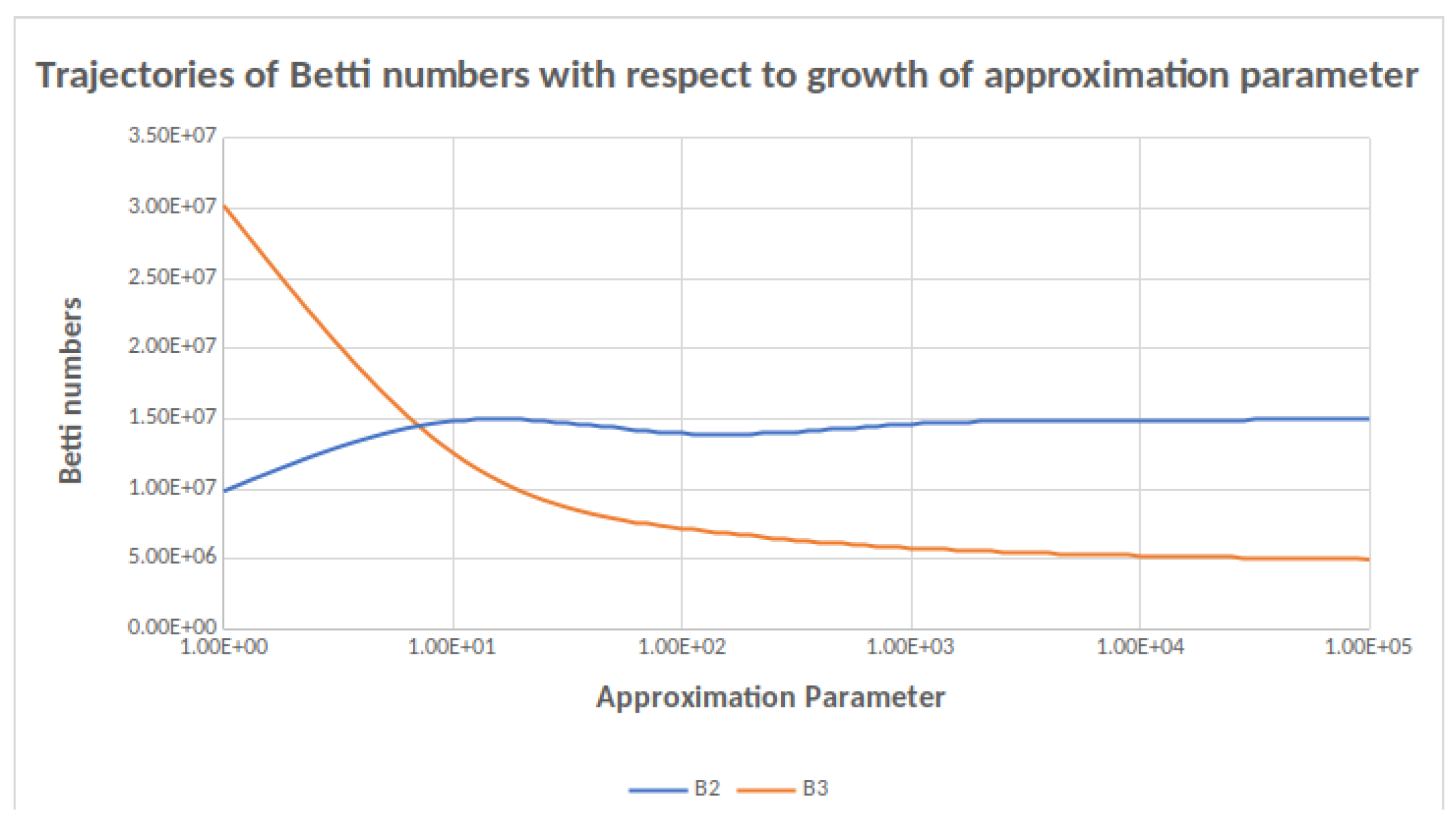
To address this problem, Flagser includes an extremely useful feature: The Approximate function. In general when one performs data analysis computation, the order of magnitude of a specific homology module is much more important that the precise value of the Betti number in question. The Approximate function allows the homology computation part of the program to compute Betti numbers and persistent homology within a user defined accuracy, and as a result dramatically reduce compute time. With Flagser we are able to perform the construction of the directed flag complex of the neocortical column of a rat [5] on a laptop within less than 30 s, and compute a good approximation for its homology within a few of hours on an HPC cluster (

Table 1. Performance of Flagser on a variety of datasets: BE = Windsurfers, GP = Google+, IN = Infectious, JA = Jazz, MQ = Macaques, PR = Protein, FN = 19th step of the Rips filtration of the 40-cycle graph, BB = Blue Brain Project neocortical column, BA = Barabási–Albert graph, CE = C-Elegans, ER = Erdős-Rényi graph. In all cases density is given as connection probability as percentage. Dataset${}^{†}$ means that the Approximate function of Flagser was used with approximation parameter 100,000. Dataset ${}^{*}$ means that the homology computation was made on a single core of an HPC cluster.

Dataset	Vertices	Edges	Density	$\mathtt{Flagser}-\mathtt{Count}$		$\mathtt{Flagser}\mathtt{Homology}$
BE	43	336	18.172	0.01 s,	3.32 MB	0.08 s,	3.81 MB
GP	23.6 K	39.2 K	0.007	0.50 s,	564.40 MB	2.09 s,	569.54 MB
IN	410	2765	1.644	0.04 s,	3.68 MB	1.27 s,	9.13 MB
JA *	198	2742	6.994	49.63 s,	3.57 MB	10 h 44 min 3.00 s,	75.79 GB
MQ	62	1187	30.879	0.09 s,	3.44 MB	9.41 s,	50.22 MB
PR	2239	6452	0.129	0.04 s,	8.63 MB	0.07 s,	9.17 MB
FN	40	760	47.500	2 min 23.26 s,	3.46 MB	Unfinished in 24 h
BB ${}^{†,}$*	31.3 K	7.8 M	0.793	23.76 s,	1.08 GB	12 h 15 min 3.00 s,	52.96 GB
BA	280	1911	2.437	0.00 s,	3.52 MB	0.03 s,	3.84 MB
CE	279	2194	2.819	0.02 s,	3.55 MB	0.12 s,	4.55 KB
ER ${}^{†}$	31.3 K	7.9 M	0.804	15.06 s,	1.08 GB	1 h 30 min 51.00 s,	4.98 GB

). Such computations were completely out of reach before. The accuracy parameter for the Approximate function can be modified to suit requirements. Experimentation suggests (although we cannot prove it in general) that the actual accuracy of computations that use the Approximate function is much higher than the accuracy theoretically guaranteed (see Figure 1).

Flagser has a built-in flexible way of associating weights to vertices and/or edges in a given graph, and the capability to have user defined weight functions that allow filtering the complex in question in a variety of ways. In particular this flexibility allows combining weights that arise from different features of the data to create a single filtration on the complex. Flagser also contains the capability of computing homology with coefficients in odd characteristics.

The directed flag complex is only one of the topological constructions one may associate with a directed graph. Motivated by more recent ideas we developed modifications of Flagser: Flagser-Count, Tournser, and Deltser (see Section 2.3 for detail).

2.1. Sample Computations

In this section we present some sample computations carried out using Flagser. Almost all computations were done on a laptop PC with 32 GB of RAM and a 2-core processor. The data files were either taken from online public domain sources or generated for the purpose of computation, as detailed below.

The first column in Table 1 contains code names for the datasets examined. The first six datasets were taken from the public domain Koblenz Network Collection (KONECT) [11,12]. We chose the following datasets (with no intention of any analysis but the performance of Flagser):

• BE = HumanContact/Windsurfers—An undirected network containing interpersonal contacts between windsurfers in southern California during the fall of 1986,
• GP = Social/Google+—A directed network that contains Google+ user to user links,
• IN = HumanContact/Infectious—face-to-face behavior of people during the exhibition INFECTIOUS: STAY AWAY in 2009 at the Science Gallery in Dublin,
• JA = HumanSocial/Jazz musicians—collaboration network between Jazz musicians,
• MQ = Animal/Macaques—A directed network containing dominance behaviour in a colony of 62 adult female Japanese macaques,
• PR = Metabolic/Human protein (Figeys)—a network of interactions between proteins in humans.

The first, second, third, and fourth columns contain information about the number of vertices, edges and connection density (in percentage), respectively. The fifth column shows the performance in terms of time and memory usage of Flagser-Count—the part of Flagser that counts the simplices in the complex it builds. The sixth column shows the same with respect to Flagser’s performance in homology computation.

One remarkable dataset among those is the set JA encoding a collaboration network between jazz musicians (an edge between two musicians if they played together). While this network is rather small and not particularly dense, computations with it required markedly more time and resources. This could be explained by the observation that the associated directed flag complex is 30-dimensional, with more than 150 million 14-dimensional simplices and similarly large numbers in neighbouring dimensions. Homology computation that took almost 11 h and required more than 75 GB of memory yielded a rather curious result with Betti numbers 1, 6, 1 in dimensions 0, 1, 2, respectively. This indicates homological simplicity is not advantageous in computation time. Two of the networks came as weighted graphs, which allowed us to compute persistent homology in those two cases (

Table 2. Performance of Flagser computing persistence.

Dataset	$\mathtt{Persistence}$
BE	00.09 s,     03.91 MB
MQ	11.47 s,     69.54 MB

). The filtration was determined by assigning to each simplex the maximal weight of an edge it contains.

The last five datasets are:

• FN = 19th step of the Rips filtration of the 40-cycle graph (equipped with the graph metric), i.e., the graph with 40 vertices, where each vertex is connected to all others except the vertex with graph distance exactly 20 from itself,
• BB = sample of a Blue Brain Project reconstruction of the neocortical column of a rat [6],
• CE = a C. Elegans brain network [13], and
• BA = a Barabási-Albert graph with a similar number of vertices and connection probability as a C. Elegans brain network.
• ER = an Erdős-Rényi graph with a similar number of vertices and connection probability as such a network,

The set FN is again an example of how large dimensionality affects computation time. In this case one knows by general theory [14] that the resulting flag complex is a model for the 19-sphere, and so the nontrivial Betti numbers occur only in dimensions 0 and 19, and they are 1 in both. However, due to the size of the complex ($2^{20}$ 19-simplices and nearly 200 million 9-simplices) we were not able to obtain a homology computation within 24 h.

In Table 1 two of the computations (see †) were done by Flagser with Approximation parameter 100,000 (the code stops reducing a column after 100,000 steps). Two computation (see *) were made on a single core of an HPC cluster to satisfy the high memory requirement.

Next, we tested the performance of Flagser with respect to several values of the Approximate parameter. We performed the computation on two graphs: (a) a Blue Brain Project neocortical column reconstruction, denoted above by BB (

Table 3. Performance of Flagser on the Blue Brain Project graph with respect to different values of the Approximate parameter. The Betti numbers computed are an approximation to the true Betti numbers. See Table 4 for accuracy.

Approx.	Time	Memory	${\mathit{\beta }}_1$	${\mathit{\beta }}_2$	${\mathit{\beta }}_3$	${\mathit{\beta }}_4$	${\mathit{\beta }}_5$
1	40 min 44 s	11.77 GB	14,640	9,831,130	30,219,098	513,675	785
10	38 min 44 s	11.96 GB	15,148	14,831,585	12,563,309	13,278	40
100	40 min 29 s	12.69 GB	15,188	13,956,297	7,171,621	9898	37
1000	55 min 40 s	15.42 GB	15,283	14,598,249	5,780,569	9822	37
10,000	2 h 24 min 17 s	23.78 GB	15,410	14,872,057	5,219,666	9821	37
100,000	12 h 15 min 3 s	52.96 GB	15,438	14,992,658	4,951,674	9821	37

and

Table 4. Number of skipped columns of the coboundary matrix for the Blue Brain Project graph with respect to different values of the Approximate parameter. The approximation accuracy of ${\beta }_i$ depends theoretically on the number of columns skipped in the coboundary matrices for ${\delta }_{i-1}$ and ${\delta }_i$.

Approx.	${\mathit{\delta }}_1$	${\mathit{\delta }}_2$	${\mathit{\delta }}_3$	${\mathit{\delta }}_4$	${\mathit{\delta }}_5$
1	7,724,934	56,746,602	19,092,109	664,481	4162
10	6,714,811	15,944,792	796,559	372	0
100	179,794	4,107,019	6414	0	0
1000	14,209	1,902,229	42	0	0
10,000	1002	1,054,397	0	0	0
100,000	27	664,857	0	0	0

), and an Erdős-Rényi graph with the same number of vertices and connection probability (

Table 5. Performance of Flagser on an Erdős-Rényi graph with respect to different values of the Approximate parameter. The Betti numbers range from dimension 0 to dimension 3.

Approx.	Time	Memory	${\mathit{\beta }}_0$	${\mathit{\beta }}_1$	${\mathit{\beta }}_2$	${\mathit{\beta }}_3$
1	4 min 45 s	3.25 GB	1	19,675	14,675,052	40
10	4 min 31 s	3.10 GB	1	19,981	9,204,135	4
100	4 min 44 s	3.18 GB	1	19,981	8,074,149	4
1000	5 min 48 s	3.33 GB	1	19,981	7,921,730	4
10,000	14 min 18 s	3.72 GB	1	19,982	7,876,858	4
100,000	1 h 30 min 51 s	4.98 GB	1	19,984	7,857,917	4

and

Table 6. Number of skipped columns of the coboundary matrix for an Erdős-Rényi graph with respect to different values of the Approximate parameter in dimensions from 1 to 3.

Approx.	${\mathit{\delta }}_1$	${\mathit{\delta }}_2$	${\mathit{\delta }}_3$
1	7,692,010	719,041	124
10	1,501,909	3	0
100	371,920	0	0
1000	219,501	0	0
10,000	174,628	0	0
100,000	155,685	0	0

). These computations were carried out on a single core of an HPC cluster.

Consider for example ${\beta }_4$. By Table 3 and Table 4 the true value is ${\beta }_4=9821$, since in that case no columns are skipped in ${\delta }_3$ and ${\delta }_4$. Thus perfect accuracy is achieved with Approximate parameter 10,000. However, with Approximate parameters 1000 and 100 one has a theoretical error of 42 and 6414 respectively, whereas the actual error is 1 and 77 respectively. In the case of ${\beta }_2$ we do not know the actual answer. However, since the total number skipped with Approximate parameter 100,000 is 664,884, and the approximate value computed for ${\beta }_2$ is 14,992,658, the calculation is accurate within less than $\pm 5\%$. Similarly, ${\beta }_1$ is computed to be 15,438 with 27 skipped columns, which stands for an accuracy at least as good as $\pm 0.2\%$. For ${\beta }_3$ the theoretical bound is clearly not as good, but here as in all other cases where precise computation was not carried out, the trajectory of the approximated Betti numbers as the approximation parameter grows suggests that the number computed is actually much closer to the real Betti numbers than the theoretical error suggests (Figure 1).

We performed a similar computation with an Erdős-Rényi random directed graph with the same number of vertices as the Blue Brain Project column and the same average probability of connection (Table 5 and Table 6). Notice that there was a very substantial difference in performance between the Blue Brain Project graph and a random graph with the same size and density parameters. The difference can be explained by the much higher complexity of the Blue Brain Project graph, as witnessed by the Betti numbers.

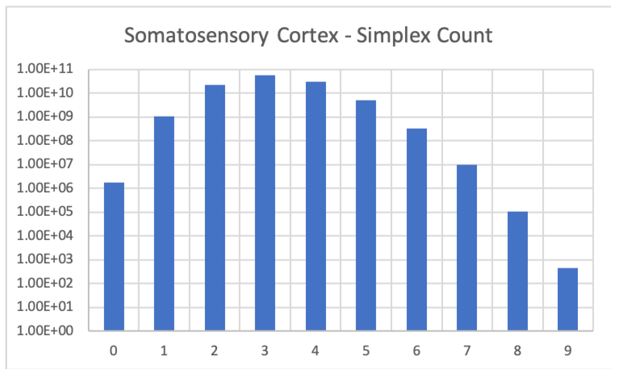
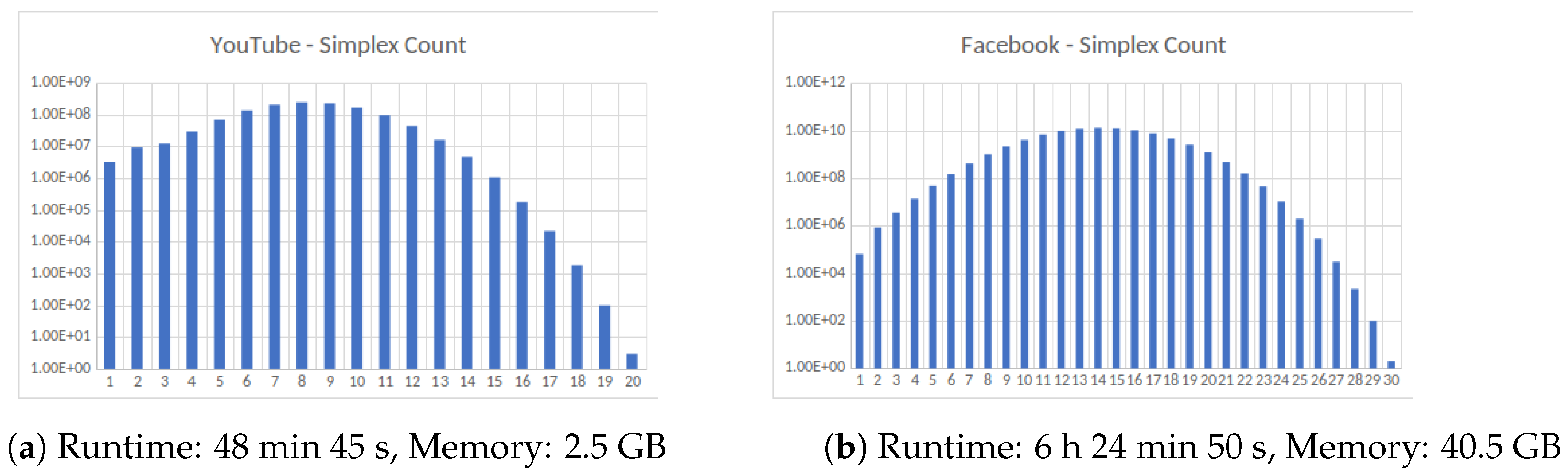
A remarkable feature of Flagser is its parallelisable construction algorithm of the directed flag complex. To demonstrate the capability of the software, we computed some large scale examples. In particular, we computed the cell counts of two sample circuits produced by the Blue Brain Project. The first is a reconstruction of the somatosensory cortex of a rat (Figure 2), and the second is the so called PL region [8] of the reconstruction of the full neocortex of a mouse (Figure 3). We also computed the simplex counts on some large non-biological networks (Figure 4).

The somatosensory cortex (Figure 2) is a digraph with about 1.7 million vertices and 1.1 billion edges (average connection probability $0.04\%$). The Blue Brain Project model of the full mouse cortex is available online [8]. The full reconstruction consists of approximately 10 million neurons. Its synaptic connections fall into three categories. Local (short distance) connections, intermediate distance connections and long distance connections. We computed the cell count of the PL region of the left hemisphere in the reconstruction, consisting of approximately 64,000 neurons and 17.5 million local connections (average connection probability $0.4\%$). We did not consider any connections but the local ones.

Interestingly the number of neurons in the model of the PL region [8] is roughly twice that in the reconstruction of the neocortical column studied in [6], and the probability of connection is roughly half. Hence we expected a comparable performance of Flagser. The results are therefore quite surprising. The likely reason for the difference in computation speeds is the higher dimensionality of the model of neocortex of the mouse, resulting in a gigantic number of simplices in the middle dimensions (approximately 1.1 trillion 11-dimensional simplices), compared to the neocortical column of the rat, with the former containing simplices of dimension 21 (see Figure 3) and the latter only containing simplices up to dimension seven.

These computation were done on an adapted version of Flagser available at [9]. This alternate version has been adapted in the following ways: the code to compute homology is removed as this is not needed, the option to load the graph from compressed sparse matrix format is included as this speeds up the time required to read the graph, the graph can be stored using Google’s dense hash map to reduce the memory needed for very large graphs, and partial results are printed during run time which allows for the computation to be resumed if it is stopped (for example, if the process is killed due to time limitations on HPC).

2.2. Comparisons

We end this section by comparing the performance of Flagser in homology computations to that of Gudhi, which is recognised as another state of the art computational software package. In doing so we are forced to restrict attention to undirected graphs, since Gudhi is designed to work only with simplicial complexes. In addition, while Flagser takes a directed graph as input and produces the complex in unison with the computation of homology, Gudhi must be given the complex as its input on which it performs its computation. Thus we combine Gudhi with the python package NetworkX which contains state of the art clique finding algorithms for undirected graphs. More specifically, we apply the find_cliques method of NetworkX to get the maximal cliques of the graph and insert these into a Gudhi SimplexTree, and then compute the homology using Gudhi. Furthermore, as NetworkX does not allow for parallel enumeration of cliques, for a fair comparison we only enable Flagser to use a single core.

In

Table 7. A comparison of the run times of Flagser and Gudhi+NetworkX to compute the homology of the undirected flag complex of six undirected graphs. Where DNF denotes the computation did not finish in under 24 h, Approx. 100,000 denotes the use of the Approximate function of Flagser with value 100,000, and MD = 6 denotes the use of the max dimension option of Flagser to compute only up to dimension 6. In the cases where the max dimension option was used, the computation did not finish within 24 h without it. All computations were done on an HPC cluster using a single CPU. The BBP layers are taken from the Blue Brain Project website [1] and the other circuits are taken from KONECT [11]. We consider the graphs as simple undirected graphs for these computations, as such the edge counts in the table above may differ from the original graphs as reciprocal edges and loops were removed.

Dataset	Vertex Count	Edge Count	Gudhi+NetworkX	Flagser
C. Elegans	279	2194	1.229 s, 585 MB	0.705 s, 589 MB
BBP Layer 2	3416	132,309	11 s, 919 MB	145 s, 745 MB
BBP Layer 5	6114	756,107	DNF	DNF
PGP	10,680	24,316	3 h 6 min 20 s, 92 GB	3 h 25 min 46 s, 5.4 GB (MD = 6)
OpenFlights	2939	19,256	DNF	3 h 45 min 18 s, 5.2 GB (MD = 6)
SimpleWiki	100,312	824,968	DNF	DNF
Dataset	Flagser (Approx. 100,000)		Betti Numbers	Approx. Betti Numbers
C. Elegans	0.701 s, 524 MB		[1, 162, 83]	[1, 162, 83]
BBP Layer 2	129 s, 612 MB		[1, 5290, 106,360, 5]	[1, 5288, 106,381, 5]
BBP Layer 5	13 h 4 min 45 s, 1.4 GB		Unknown	[1, 1222, 1,427,597, 1133]
PGP	3 h 30 min 32 s, 5.3 B (MD = 6)		[1, 1093, 22, 1]	[1, 1093, 22, 1, 0, 0, 0]
OpenFlights	3 h 37 min 19 s, 5.3 GB (MD = 6)		[24,354, 310, 107, 53, 2, 2,0]	[24,354, 309, 108, 53, 4, 2, 0]
SimpleWiki	15 h 7 min 41 s, 21.0 GB (MD = 6)		Unknown	[304, 125,571, 45,306, 31,866, 10,486, 319, 6]

we compare the run time of Gudhi+NetworkX with Flagser. We can see that for small examples such as C. Elegans and BBP layer two the times and memory usage are fairly similar, although Gudhi+NetworkX is a bit faster on BBP layer two. We can also see that Gudhi+NetworkX was faster on the PGP graph, with Flagser not finishing without the max dimension option. Although for this graph we can see that Gudhi+NetworkX required 92 GB of memory, whereas using max dimension with Flagser only required 5.4 GB. For the OpenFlights and SimpleWiki graphs neither Gudhi+NetworkX nor Flagser finished. However, if we use the max dimension option with Flagser we can compute the homology of OpenFlights (up to dimension 6) in under four hours using only 5.2 GB of memory. Similarly, for SimpleWiki if we use both the Approximate and max dimension option, then we can get results in under 24 h, on a graph with over 100k vertices.

To provide a more complete picture, we recorded in

Table 8. The precise number of columns skipped in the Flagser computations presented in Table 7. The notation ${\delta }_i$ refers to the i-th coboundary operator.

Dataset	${\mathit{\delta }}_1$	${\mathit{\delta }}_2$	${\mathit{\delta }}_3$	${\mathit{\delta }}_4$	${\mathit{\delta }}_5$	${\mathit{\delta }}_6$	${\mathit{\delta }}_7$
C. Elegans	0	0	0	0	0	0	0
BBP2	0	23	0	0	0	0	0
BBP5	0	32	49,614	0	0	0	0
PGP	0	0	0	0	0	0	0
OpenFlights	0	2	0	2	0	0	0
SimpleWiki	0	56	1357	1280	63	0	0

the actual number of columns skipped in each of the computations in Table 7.

We add that although Gudhi+NetworkX is the closest state of the art comparison to Flagser we are aware of, it does not allow for the use of some of the key advantages of Flagser, such as parallelisation and working with directed graphs and ordered simplicial complexes. Moreover, we are unaware of any faster algorithm for the enumeration of directed cliques than the breadth first search approach applied by Flagser.

We also considered some older computational packages publically available, although we did not perform our own tests on those packages. A notable example is the ground breaking work of Zomorodian [15], designed for fast computation of the Vietoris–Rips complex of a dataset. That code boasts a computation of the three-dimensional complex for a point cloud of 10,000 points uniformly sampled on a unit 2-sphere in ${\mathbb{R}}^3$ with parameter $ϵ=0.15$, resulting in a complex with roughly 24 M simplices in approximately 80 s, using two dual core processors running under Linux. By comparison, see BB and ER in Table 1, where we apply Flagser-Count to an early Blue Brain Project reconstruction of brain tissue. This is a graph with approximately 31 K vertices and 8 M edges, resulting in a seven-dimensional directed flag complex with roughly 160 M simplices. The computations were done on a laptop PC with a single dual core processor under Microsoft Windows 10 and completed in 23.76 s, using a mere 1.08 GB of memory. For a comparable Erdős-Rényi graph the computation is done in just above 15 s. It should also be noted that Zomorodian’s software uses approximation methods in the construction of the complex for gained speed. By contrast, Flagser produces an exact flag complex but uses controlled approximation in homology computation (see Section 4.4.2), and as such it is unique to the best of our knowledge.

Another computational package worth mentioning is jHoles [16]. jHoles takes as input a weighted (undirected) graph, filters it by subgraphs, based on the weights, and then proceeds to find maximal cliques in each stage of the filtration. In this way a filtered simplicial complex is obtained. Computation of persistent homology is then performed using JavaPlex, which at the point of publication of [16] was one of the fastest implementations for computing persistent homology. The performance of jHoles in creating the complexes is measured by comparison to an earlier version Holes as a function of the average number of steps and average number of arches of sample graphs. jHoles is shown to perform remarkably better than Holes. We did not perform a comparative analysis for Flagser.

2.3. Availability of Source Code

Flagser was developed as a part of an EPSRC funded project on applications of topology in neuroscience. As such Flagser is an open source package, licensed under the LGPL 3.0 scheme. The code can be found on the GitHub page of Daniel Lütgehetmann who owns the copyright for the code and will maintain the page [17].

In the course of using Flagser in the project three adapted versions were developed, and can be found in the GitHub page of Jason Smith [9], who will maintain the page. The following modifications are available.

• Flagser-Count: A modification of a basic procedure in Flagser, optimised for very large networks.
• Deltser: A modification of Flagser that computes persistent homology on any finite delta complex (like a simplicial complex, except more than one simplex may be supported on the same set of vertices).
• Tournser: The flag tournaplex of a directed graph is the delta complex whose simplices are all tournaments that occur in the graph. Tournser is an adaption of Flagser which computes (persistent) homology of the tournaplex of a finite directed graph. Tournser uses two filtrations that occur naturally in tournaplexes, but can also be used in conjunction with other filtrations.

3. Discussion

Flagser is designed specifically to work with directed graphs, and to the best of our knowledge is the only comprehensive package with this capability. Hence it is not easily comparable to other computational software. In Section 2.2 we attempted a fair comparison of the performance of Flagser in homology computations for flag complexes of certain undirected graphs to that of a combined package of Gudhi+NetworkX. There we attempted to explain the advantages and limitations of Flagser. In spite of the fact that Gudhi+NetworkX is sometimes significantly faster in creating a flag complex and computing its homology, we demonstrated by means of examples that there are graphs for which Gudhi+NetworkX does not terminate and Flagser does, and other examples where neither terminates but the Approximate function of Flagser allows a computation within a reasonable margin of error (see Section 2.1).

It is clear that Flagser can be developed further. In particular, the comparison of the speed of its homology computation capability with that of Gudhi suggests that Flagser could potentially benefit from an advanced reduction algorithm of the kind used by Gudhi prior to computation of homology. However, this would require committing the complex to memory, which will dramatically increase the memory cost of the code. It would also be useful to build an option for predicted accuracy of the homology computation when the Approximate function is used, but we were not able to do so.

The usefulness of Flagser and its derivatives is clearly not limited to neuroscience. Topological analysis of graphs and complexes arising in both theoretical problems and applicable studies have become quite prevalent in recent years [18,19]. Hence Flagser, in its original or modified form, could become a major computational aid in many fields. Flagser and its modifications are open source packages, licensed under the LGPL 3.0 scheme, and can be accessed through the developers GitHub pages. See Section 2.3 for details. In particular, documentation for Flagser, including examples, tools and code options can be found in [17].

4. Materials and Methods

4.1. Mathematical Background

In this section, we give a brief introduction to directed flag complexes of directed graphs, and to persistent homology. For more detail, see [6,20,21].

Definition 1.

A graph G is a pair $(V,E)$, where V is a finite set referred to as the vertices of G, and E is a subset of the set of unordered pairs $e=\{v,w\}$ of distinct points in V, which we call the edges of G. Geometrically the pair $\{u,v\}$ indicates that the vertices u and v are adjacent to each other in G. A directed graph, or a digraph, is similarly a pair $(V,E)$ of vertices V and edges E, except the edges are ordered pairs of distinct vertices, i.e., the pair $(v,w)$ indicates that there is an edge from v to w in G. In a digraph we allow reciprocal edges, i.e., both $(u,v)$ and $(v,u)$ may be edges in G, but we exclude loops, i.e., edges of the form $(v,v)$.

Next we define the main topological objects considered in this article.

Definition 2.

An abstract simplicial complex on a vertex set V is a collection X of non-empty finite subsets $\sigma \subseteq V$ that is closed under taking non-empty subsets. An ordered simplicial complex on a vertex set V is a collection of non-empty finite ordered subsets $\sigma \subseteq V$ that is closed under taking non-empty ordered subsets. Notice that the vertex set V does not have to have any underlying order. In both cases the subsets σ are called the simplices of X, and σ is said to be a k-simplex, or a k-dimensional simplex, if it consists of $k+1$ vertices. If $\sigma \in X$ is a simplex and $\tau \subseteq \sigma$, then τ is said to be a face of σ. If τ is a subset of V (ordered if X is an ordered simplicial complex) that contains σ, then τ is called a coface of σ. If $\sigma =(v_0,\dots ,v_k)$ is a k-simplex in X, then the i-th face of σ is the subset ${\partial }_i\left(\sigma \right)=(v_0,\dots ,{\widehat{v}}_i,\dots ,v_k)$ where by ${\widehat{v}}_i$ we mean omit the i-th vertex. For $d\ge 0$ denote by $X_d$ the set of all d-dimensional simplices of X.

Notice that if X is any abstract simplicial complex with a vertex set V, then by fixing a linear order on the set V, we may think of each one of the simplices of X as an ordered set, where the order is induced from the ordering on V. Hence any abstract simplicial complex together with an ordering on its vertex set determines a unique ordered simplicial complex. Clearly any two orderings on the vertex set of the same complex yield two distinct but isomorphic ordered simplicial complexes. Hence from now on we may assume that any simplicial complex we consider is ordered.

Definition 3.

Let $G=(V,E)$ be a directed graph. The directed flag complex $dFl\left(G\right)$ is defined to be the ordered simplicial complex whose k-simplices are all ordered $(k+1)$-cliques, i.e., $(k+1)$-tuples $\sigma =(v_0,v_1,\dots ,v_k)$, such that $v_i\in V$ for all i, and $(v_i,v_j)\in E$ for $i<j$. The vertex $v_0$ is called the initial vertex of σ or the source of σ, while the vertex $v_k$ is called the terminal vertex of σ or the sink of σ.

Let $\mathbb{F}$ be a field, and let X be an ordered simplicial complex. For any $k\ge 0$ let $C_k\left(X\right)$ be the $\mathbb{F}$-vector space with basis given by the set $X_k$ of all k-simplices of X. If $\sigma =(v_0,\dots ,v_k)$ is a k-simplex in X, then the i-th face of $\sigma$ is the subset ${\partial }_i\left(\sigma \right)=(v_0,\dots ,{\widehat{v}}_i,\dots ,v_k)$, where ${\widehat{v}}_i$ means that the vertex $v_i$ is removed to obtain the corresponding $(k-1)$-simplex. For $k\ge 1$, define the k-th boundary map $d_k:C_k\left(X\right)\to C_{k-1}\left(X\right)$ by

$$d_k\left(\sigma \right)=\sum _{i=0}^k{(-1)}^i{\partial }_i\left(\sigma \right)\in C_{k-1}\left(X\right).$$

The boundary map has the property that $d_k\circ d_{k+1}=0$ for each $k\ge 1$ [21]. Thus $Im\left(d_{k+1}\right)\subseteq Ker\left(d_k\right)$ and one can make the following fundamental definition:

Definition 4.

Let X be an ordered simplicial complex. The k-th homology group of X (over $\mathbb{F}$) denoted by $H_k\left(X\right)=H_k(X;\mathbb{F})$ is defined to be

$$H_k\left(X\right)=Ker\left(d_k\right)/Im\left(d_{k+1}\right).$$

If X is an ordered simplicial complex, and $Y\subseteq X$ is a subcomplex, then the inclusion $\iota :Y\to X$ induces a chain map ${\iota }_{*}:C_{*}\left(Y\right)\to C_{*}\left(X\right)$, i.e., a homomorphism ${\iota }_k:C_k\left(Y\right)\to C_k\left(X\right)$ for each $k\ge 0$, such that $d_k\circ {\iota }_k={\iota }_{k-1}\circ d_k$. Hence one obtains an induced homomorphism for each $k\ge 0$,

$${\iota }_{*}:H_k\left(Y\right)\to H_k\left(X\right).$$

This is a particular case of a much more general property of homology, namely its functoriality with respect to so called simplicial maps. We will not however require this level of generality in the discussion below.

Definition 5.

A filtered simplicial complex is a simplicial complex X together with a filter function $f:X\to \mathbb{R}$, i.e., a function satisfying the property that if σ is a face of a simplex τ in X, then $f\left(\sigma \right)\le f\left(\tau \right)$. Given $b\in \mathbb{R}\bigsqcup \{\infty \}$, define the sublevel complex $X\left[b\right]$ to be the inverse image $f^{-1}\left((-\infty ,b]\right)$.

Notice that the condition imposed on the function f in Definition 5 ensures that for each $b\in \mathbb{R}\bigsqcup \{\infty \}$, the sublevel complex $X\left[b\right]$ is a subcomplex of X, and if $b\le b^{\prime }$ then $X\left[b\right]\subseteq X\left[b^{\prime }\right]$. By default we identify X with $X[\infty ]$. Thus a filter function f as above defines an increasing family of subcomplexes $X\left[b\right]$ of X that is parametrised by the real numbers.

If the values of the filter function f are a finite subset of the real numbers, as will always be the case when working with actual data, then by enumerating those numbers by their natural order we obtain a finite sequence of subspace inclusions

$$X\left[1\right]\subseteq X\left[2\right]\subseteq \cdots \subseteq X\left[n\right]=X.$$

For such a sequence one defines its persistent homology as follows: for each $i\le j$ and each $k\ge 0$ one has a homomorphism

$$h_k^{i,j}:H_k\left(X\left[i\right]\right)\to H_k\left(X\left[j\right]\right),$$

induced by the inclusion $X\left[i\right]\to X\left[j\right]$. The image of this homomorphism is a k-th persistent homology group of X with respect to the given filtration, as it represents all homology classes that are present in $H_k\left(X\left[i\right]\right)$ and carry over to $H_k\left(X\left[j\right]\right)$. To use the common language in the subject, $Im\left(h_k^{i,j}\right)$ consists of the classes that were “born” at or before filtration level i and are still “alive” at filtration level j. The rank of $Im\left(h_k^{i,j}\right)$ is a persistent Betti number for X and is denoted by ${\beta }_k^{i,j}$.

Persistent homology can be represented as a collection of persistence pairs, i.e., pairs $(i,j)$, where $0\le i<j\le n$. The multiplicity of a persistence pair $(i,j)$ in dimension k is, roughly speaking, the number of linearly independent k-dimensional homology classes that are born in filtration i and die in filtration j. More formally,

$${\mu }_k^{i,j}=({\beta }_k^{i,j-1}-{\beta }_k^{i-1,j-1})-({\beta }_k^{i,j}-{\beta }_k^{i-1,j}).$$

Persistence pairs can be encoded in persistence diagrams or persistence barcodes. See [22] for more detail.

Flagser computes the persistent homology of filtered directed flag complexes. The filtration of the flag complexes is based on filtrations of the 0-simplices and/or the 1-simplices, from which the filtration values of the higher dimensional simplices can then be computed by various formulas. When using the trivial filtration algorithm of assigning the value 0 to each simplex, for example, Flagser simply computes the ordinary simplicial Betti numbers. The software uses a variety of tricks to shorten the computation time (see below for more details), and outperforms many other software packages, even for the case of unfiltered complexes (i.e., complexes with the trivial filtration). In the following, we mainly focus on (persistent) homology with coefficients in finite fields, and if we don’t mention it explicitly we consider the field with two elements ${\mathbb{F}}_2$.

4.2. Representing the Directed Flag Complex in Memory

An important feature of Flagser is its memory efficiency which allows it to carry out rather large computations on a laptop with a mere 16 GB of RAM (see controlled examples in Section 2). In order to achieve this, the directed flag complex of a graph is generated on the fly and not stored in memory. An n-simplex of the directed flag complex $dFl\left(G\right)$ corresponds to a directed $(n+1)$-clique in the graph $G=(V,E)$. Hence each n-simplex is identified with its list of vertices ordered by their in-degrees in the corresponding directed clique from 0 to n. The construction of the directed flag complex is performed by a double iteration:

• For an arbitrary fixed vertex $v_0\in V$, we iterate over all simplices which have $v_0$ as the initial vertex.
• Iterate Step 1 over all vertices (but see 3 below).

This procedure enumerates all simplices exactly once.

In more detail, consider a fixed vertex $v_0$. The first iteration of Step 1 starts by finding all vertices w such that there exists a directed edge from $v_0$ to w. This produces the set $S_1^{v_0}$ of all 1-simplices of the form $(v_0,w)$, i.e., all 1-simplices that have $v_0$ as their initial vertex. In the second iteration of Step 1, construct for each 1-simplex $(v_0,v_1)\in S_1^{v_0}$ obtained in the first iteration, the set $S_2^{v_0,v_1}$ by finding the intersection of the two sets of vertices that can be reached from $v_0$ and $v_1$, respectively. In other words,

$$S_2^{v_0,v_1}=\{w\in V|(v_0,w)\in S_1^{v_0},\mathrm{and}(v_1,w)\in S_1^{v_1}\}.$$

This is the set of all 2-simplices in $dFl\left(G\right)$ of the form $(v_0,v_1,w)$. Proceed by iterating Step 1, thus creating the prefix tree of the set of simplices with initial vertex $v_0$. The process must terminate, since the graph G is assumed to be finite. In Step 2 the same procedure is iterated over all vertices in the graph (under the constraint described in 3 below.)

This algorithm has three main advantages:

• The construction of the directed flag complex is very highly parallelisable. In theory one could use one CPU for each of the vertices of the graph, so that each CPU computes only the simplices with this vertex as initial vertex.
• Only the graph is loaded into memory. The directed flag complex, which is usually much bigger, does not have any impact on the memory footprint.
• The procedure skips branches of the iteration based on the prefix. The idea is that if a simplex is not contained in the complex in question, then no simplex containing it as a face can be in the complex. Therefore, if we computed that a simplex $(v_0,\dots ,v_k)$ is not contained in our complex, then we don’t have to iterate Step 1 on its vertices to compute the vertices w that are reachable from each of the $v_i$. This allows us to skip the full iteration branch of all simplices with prefix $(v_0,\dots ,v_k)$. This is particularly useful for iterating over the simplices in a subcomplex.

In the code, the adjacency matrix (and for improved performance its transpose) are both stored as bitsets (Bitsets store a single bit of information (0 or 1) as one physical bit in memory, whereas usually every bit is stored as one byte (8 bit). This representation improves the memory usage by a factor of 8, and additionally allows the compiler to use much more efficient bitwise logical operations, like “AND” or “OR”. Example of the bitwise logical “AND” operation: 0111 and 1101 = 0101). This makes the computation of the directed flag complex more efficient. Given a k-simplex $(v_0,\dots ,v_k)$ in $dFl\left(G\right)$, the set of vertices

$$\{w\in V|(v_0,\dots ,v_k,w)\in dFl\left(G\right)\}$$

is computed as the intersection of the sets of vertices that the vertices $v_0,\dots ,v_k$ have a connection to. Each such set is given by the positions of the 1’s in the bitsets of the adjacency matrix in the rows corresponding to the vertices $v_0,\dots ,v_k$, and thus the set intersection can be computed as the logical “AND” of those bitsets.

In some situations, we might have enough memory available to load the full complex into memory. For these cases, there exists a modified version of the software that stores the tree described above in memory, allowing to

• perform computations on the complex such as counting, or computing co-boundaries etc., without having to recompute the intersections described above, and
• associate data to each simplex with fast lookup time.

The second part is useful for assigning unique identifiers to each simplex. Without the complex in memory a hash map with custom hashing function has to be created for this purpose, which slows down the lookup of the global identifier of a simplex dramatically.

4.3. Computing the Coboundaries

In Ripser, [10], cohomology is computed instead of homology. The reason for this choice is that for typical examples, the coboundary matrix contains many more columns that can be skipped in the reduction algorithm than the boundary matrix [23].

If $\sigma$ is a simplex in a complex X, then $\sigma$ is a canonical basis element in the chain complex for X with coefficients in the field $\mathbb{F}$. The hom-dual ${\sigma }^{*}$, i.e., the function that associates $1\in \mathbb{F}$ with $\sigma$ and 0 with any other simplex, is a basis element in the cochain complex computing the cohomology of X with coefficients in $\mathbb{F}$. The differential in the cochain complex requires considering the coboundary simplices of any given simplex, i.e., all those simplices that contain the original simplex as a face of codimension 1.

In Ripser, the coboundary simplices are never stored in memory. Instead, the software enumerates the coboundary simplices of any given simplex by a clever indexing technique, omitting all coboundary simplices that are not contained in the complex defined by the filtration stage being computed. However, this technique only works if the number of theoretically possible coboundary entries is sufficiently small. In the directed situation, and when working with a directed graph with a large number of vertices, this number is typically too large to be enumerated by a 64-bit integer. Therefore, in Flagser we pre-compute the coboundary simplices into a sparse matrix, achieving fast coboundary iteration at the expense of longer initialisation time and more memory load. An advantage of this technique is that the computation of the coboundary matrices can be fully parallelised, again splitting the simplices into groups indexed by their initial vertex.

Given an ordered list of vertex identifiers $(v_0,\dots ,v_k)$ characterising a directed simplex $\sigma$, the list of its coboundary simplices is computed by enumerating all possible ways of inserting a new vertex into this list to create a simplex in the coboundary of $\sigma$. Given a position $0\le p\le k+1$, the set of vertices that could be inserted in that position is given by the intersection of the set of vertices that have a connection from each of the vertices $v_0,\dots ,v_{p-1}$ and the set of vertices that have a connection to each of the vertices $v_p,\dots ,v_k$. This intersection can again be efficiently computed by bitwise logical operations of the rows of the adjacency matrix and its transpose (the transpose is necessary to efficiently compute the incoming connections of a given vertex).

With the procedure described above, we can compute the coboundary of every k-simplex. The simplices in this representation of the coboundary are given by their ordered list of vertices, and if we want to turn this into a coboundary matrix we have to assign consecutive numbers to the simplices of the different dimensions. We do this by creating a hash map, giving all simplices of a fixed dimension consecutive numbers starting at 0. This numbering corresponds to choosing the basis of our chain complex by fixing the ordering, and using the hash map we can lookup the number of each simplex in that ordering. This allows us to turn the coboundary information computed above into a matrix representation. If the flag complex is stored in memory, creating a hash map becomes unnecessary since we can use the complex as a hash map directly, adding the dimension-wise consecutive identifiers as additional information to each simplex. This eliminates the lengthy process of hashing all simplices and is therefore useful in situations where memory is not an issue.

4.4. Performance Considerations

Flagser is optimised for large computations. In this section we describe some of the algorithmic methods by which this is carried out.

4.4.1. Sorting the Columns of the Coboundary Matrix

The reduction algorithm iteratively reduces the columns in order of their filtration value (i.e., the filtration value of the simplex that this column represents). Each column is reduced by adding previous (already reduced) columns until the pivot element does not appear as the pivot of any previous column. While reducing all columns the birth and death times for the persistence diagram can be read off: roughly speaking, if a column with a certain filtration value $f_0$ ends up with a pivot that is the same as the pivot of a column with a higher filtration value $f_1$, then this column represents a class that is born at time $f_0$ and dies at time $f_1$. Experiments showed that the order of the columns is crucial for the performance of this reduction algorithm, so Flagser sorts the columns that have the same filtration values by an experimentally determined heuristic (see below). This is of course only useful when there are many columns with the same filtration values, for example when taking the trivial filtration where every simplex has the same value. In these cases, however, it can make very costly computations tractable.

The heuristic to sort the columns is applied as follows:

• Sort columns in ascending order by their filtration value. This is necessary for the algorithm to produce the correct results.
• Sort columns in ascending order by the number of non-zero entries in the column. This tries to keep the number of new non-zero entries that a reduction with such a column produces small.
• Sort columns in descending order by the position of the pivot element of the unreduced column. This means that the larger the pivot (i.e., the higher the index of the last non-trivial entry), the lower the index of the column is in the sorted list. The idea behind this is that “long columns”, i.e., columns whose pivot element has a high index, should be as sparse as possible. Using such a column to reduce the columns to its right is thus more economical. Initial coboundary matrices are typically very sparse. Thus ordering the columns in this way gives more sparse columns with large pivots to be used in the reduction process.
• Sort columns in descending order by their “pivot gap”, i.e., by the distance between the pivot and the next nontrivial entry with a smaller row index. A large pivot gap is desirable in case the column is used in reduction of columns to its right, because when using such a column to reduce another column, the added non-trivial entry in the column being reduced appears with a lower index. This may yield fewer reduction steps on average.

Remark 1.

We tried various heuristics—amongst them different orderings of the above sortings—but the setting above produced by far the best results. Running a genetic algorithm in order to find good combinations and orderings of sorting criteria produced slightly better results on the small examples we trained on, but it did not generalise to bigger examples. It is known that finding the perfect ordering for this type of reduction algorithm is NP-hard [24].

4.4.2. Approximate Computation

Another method that speeds up computations considerably is the use of Approximate computation. This simply means allowing Flagser to skip columns that need many reduction steps. The reduction of these columns takes the most time, so skipping even only the columns with extremely long reduction chains gives significant performance gains. By skipping a column, the rank of the matrix can be changed by at most one, so the error can be explicitly bounded. This is especially useful for computations with trivial (i.e., constant) filtrations, as the error in the resulting Betti numbers is easier to interpret than the error in the set of persistence pairs.

Experiments on smaller examples show that the theoretical error that can be computed from the number of skipped columns is usually much bigger than the actual error. Therefore, it is usually possible to quickly get rather reliable results that afterwards can be refined with more computation time. See

Table 9. Theoretical and actual error in the computation of the first Betti number by skipping the reduction of columns that require certain numbers of reduction steps. The cell counts are 4656, 35,587, and 1,485,099 in dimensions $0,1$ and 2 respectively, and the first Betti number is 3321. The computations were made as averages over ten runs on a MacBook Pro, 2.5 GHz Intel Core i7. Source of data: Blue Brain Project—Layer 4 of the neocortical column reconstruction, Version 5.

Approximation	None	${10}^4$	${10}^3$	${10}^2$	${10}^1$
Theoretical error	0	322	1380	7849	192,638
Actual error	0	0	19	58	65
Computation time	113 s	49 s	43 s	41 s	39 s

for an example of the speed-up gained by Approximate computation. The user of Flagser can specify an approximation level, which is given by a number (defaulting to infinity). This number determines after how many reduction steps the current column is skipped. The lower the number, the more the performance gain (and the more uncertainty about the result). At the current time it is not possible to specify the actual error margin for the computation, as it is very complicated to predict the number of reductions that will be needed for the different columns.

4.4.3. Dynamic Priority Queue

When reducing the matrix, Ripser stores the column that is currently reduced as a priority queue, ordering the entries in descending order by filtration value and in ascending order by an arbitrarily assigned index for entries with the same filtration value. Each index can appear multiple times in this queue, but due to the sorting all repetitions are next to each other in a contiguous block. To determine the final entries of the column after the reduction process, one has to loop over the whole queue and sum the coefficients of all repeated entries.

This design makes the reduction of columns with few reduction steps very fast but gets very slow (and memory-intensive) for columns with a lot of reduction steps: each time we add an entry to the queue it has to “bubble” through the queue and find its right place. Therefore, Flagser enhances this queue by dynamically switching to a hash-based approach if the queue gets too big: after a certain number of elements were inserted into the queue, the queue object starts to track the ids that were inserted in a hash map, storing each new entry with coefficient 1. If a new entry is then already found in the hash map, it is not again inserted into the queue but rather the coefficient of the hash map is updated, preventing the sorting issue described above. When removing elements from the front, the queue object then takes for each element that is removed from the front of the queue the coefficient stored in the hash map into account when computing the final coefficient of that index.

4.4.4. Apparent Pairs

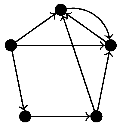
In Ripser, so-called apparent pairs are used in order to skip some computations completely. These rules are based on discrete Morse theory [25], but they only apply for non-directed simplicial complexes. Since we consider directed graphs, the associated flag complex is a semi-simplicial rather than simplicial complex, so we cannot use this simplification. Indeed, experiments showed that enabling the skipping of apparent pairs yields wrong results for directed flag complexes of certain directed graphs. For example, when applied to the directed flag complex of the graph in Figure 5, using apparent pairs gives ${\beta }_1={\beta }_2=0$ and not using apparent pairs gives ${\beta }_1={\beta }_2=1$, which is visibly the correct answer.

Experiments showed that when applied to directed flag complexes that arise from graphs without reciprocal connections (so that the resulting directed flag complex is a simplicial complex), enabling the skipping of apparent pairs does not give a big performance advantage. In fact, we found a significant reduction in run time for subgraphs of the connectome of the reconstruction of the neocortical column based data averaged across the five rats that were used in [6], the Google plus network and the Twitter network from KONECT [11].

References

- Blue Brain Project. Blue Brain Project, General Website. Available online: https://www.epfl.ch/research/domains/bluebrain (accessed on 2 July 2019).
- Laboratory for Topology and Neuroscience. Available online: https://hessbellwald-lab.epfl.ch/ (accessed on 2 July 2019).
- Maria, C.; Boissonnat, J.D.; Glisse, M.; Yvinec, M. The Gudhi Library: Simplicial Complexes and Persistent Homology; Research Report RR-8548; INRIA: Rocquencourt, France, 2014. [Google Scholar]
- Bauer, U.; Kerber, M.; Reininghaus, J.; Wagner, H. Phat—Persistent Homology Algorithms Toolbox. J. Symb. Comput. 2017, 78, 76–90. [Google Scholar] [CrossRef]
- Blue Brain Project. Digital Reconstruction of Neocortical Microcircuitry. 2019. Available online: https://bbp.epfl.ch/nmc-portal/downloads (accessed on 2 July 2019).
- Reimann, M.W.; Nolte, M.; Scolamiero, M.; Turner, K.; Perin, R.; Chindemi, G.; Dłotko, P.; Levi, R.; Hess, K.; Markram, H. Cliques of Neurons Bound into Cavities Provide a Missing Link between Structure and Function. Front. Comput. Neurosci. 2017, 11, 48. [Google Scholar] [CrossRef] [PubMed] [Green Version]
- Dłotko, P. Topological Neuroscience Software. Available online: http://neurotop.gforge.inria.fr (accessed on 2 July 2019).
- Blue Brain Project. Mouse Whole-Neocortex Connectome Model. 2019. Available online: https://portal.bluebrain.epfl.ch/resources/models/mouse-projections/ (accessed on 2 July 2019).
- Smith, J.P. Flagser-Adaptions. 2019. Available online: https://github.com/JasonPSmith/flagser-adaptions (accessed on 2 July 2019).
- Bauer, U. Ripser: A Lean C++ Code for the Computation of Vietoris-Rips Persistence Barcodes. 2015–2018. Available online: http://ripser.org (accessed on 29 August 2018).
- Kunegis, J. KONECT—The Koblenz Network Collection. In Proceedings of the 22nd International Conference on World Wide Web Companion, Rio de Janeiro, Brazil, 13–17 May 2013; pp. 1343–1350. [Google Scholar]
- Kunegis, J. KONECT—The Koblenz Network Collection Website. Available online: http://konect.uni-koblenz.de/ (accessed on 2 July 2019).
- Varshney, L.R.; Chen, B.L.; Paniagua, E.; Hall, D.H.; Chklovskii, D.B. Structural Properties of the Caenorhabditis elegans Neuronal Network. PLoS Comput. Biol. 2011, 7, e1001066. [Google Scholar] [CrossRef] [PubMed] [Green Version]
- Adamaszek, M. Special cycles in independence complexes and superfrustration in some lattices. Topol. Appl. 2013, 160, 943–950. [Google Scholar] [CrossRef]
- Zomorodian, A. Fast construction of the Vietoris-Rips complex. Comput. Graph. 2010, 34, 263–271. [Google Scholar] [CrossRef]
- Binchi, J.; Merelli, E.; Rucco, M.; Petri, G.; Vaccarino, F. jHoles: A Tool for Understanding Biological Complex Networks via Clique Weight Rank Persistent Homology. Electron. Notes Theor. Comput. Sci. 2014, 306, 5–18. [Google Scholar] [CrossRef]
- Lütgehetmann, D. Computing Homology of Directed Flag Complexes. 2019. Available online: https://github.com/luetge/flagser (accessed on 2 July 2019).
- Costa, A.; Farber, M. Large random simplicial complexes, I. J. Topol. Anal. 2016, 8, 399–429. [Google Scholar] [CrossRef] [Green Version]
- Sanchez-Garcia, R.J.; Fennelly, M.; Norris, S.; Wright, N.; Niblo, G.; Brodzki, J.; Bialek, J.W. Hierarchical spectral clustering of power grids. IEEE Trans. Power Syst. 2014, 29, 2229–2237. [Google Scholar] [CrossRef] [Green Version]
- Munkres, J.R. Elements of Algebraic Topology; Addison-Wesley: Boston, MA, USA, 1984. [Google Scholar]
- Hatcher, A. Algebraic Topology; Cambridge University Press: Cambridge, UK, 2002. [Google Scholar]
- Edelsbrunner, H.; Harer, J. Persistent homology—A survey. In Surveys on Discrete and Computational Geometry; American Mathematical Soc.: Providence, RI, USA, 2008; Volume 453, pp. 257–282. [Google Scholar] [CrossRef] [Green Version]
- Bauer, U. Ripser: Efficient Computation of Vietoris-Rips Persistence Barcodes. 2018. Available online: http://ulrich-bauer.org/ripser-talk.pdf (accessed on 29 August 2018).
- Yannakakis, M. Computing the Minimum Fill-In is NP-Complete. SIAM J. Algebraic Discret. Methods 1981, 2, 77–79. [Google Scholar] [CrossRef]
- Forman, R. Morse Theory for Cell Complexes. Adv. Math. 1998, 134, 90–145. [Google Scholar] [CrossRef] [Green Version]
Figure 1.
Trajectories of and as a function of the approximation parameter. A change in order of magnitude in the approximation parameter results in a small change in the Betti number computed.
Figure 2.
Cell count in the Blue Brain reconstruction of the somatosensory cortex. Computation was run on an HPC cluster using 256 CPUs, required 55.69 GB of memory and took 7.5 h to complete.
Figure 3.
The simplex count for the PL-Left region of a mouse neocortex (local connections only). The complex is 21-dimensional with more than 1.2 trillion 11-dimensional simplices. Computation was run in parallel on two nodes of an HPC cluster with 256 CPUs each, required 1 GB of memory and took five days to complete (run as 10 different jobs of 24 h each).
Figure 4.
Four large datasets taken from the Koblenz Network Collection [11]. (a) Social network of YouTube users and their friendship connections, (b) friendship data of Facebook users, (c) road network of the State of Texas, a node is an intersection between roads or road endpoint and edges are road segments and (d) Road network of the State of California. All computations were carried out on an HPC cluster using 256 cores.
Figure 5.
A digraph for which using apparent pairs to compute the homology of the directed flag complex gives the wrong results.