An Adaptive h-Refinement Algorithm for Local Damage Models

Abstract

An adaptive mesh refinement strategy is proposed for local damage models that often arise from internal state variable based continuum damage models. The proposed algorithm employs both the finite element method and the finite difference method to integrate the equations of motion of a linear elastic material with simple isotropic microcracking. The challenges of this problem include the time integration of coupled partial differential equations with time-dependent coefficients, and the proper choice of solution spaces to yield a stable finite element formulation. Discontinuous elements are used for the representation of the damage field, as it is believed that this reduction in regularity is more consistent with the physical nature of evolving microcracking. The adaptive mesh refinement algorithm relies on custom refinement indicators, two of which are presented and compared. The two refinement indicators we explore are based on the time rate of change of the damage field and on the energy release rate, respectively, where the energy release rate measures the energy per unit volume available for damage to evolve. We observe the performance of the proposed algorithm and refinement indicators by comparing the predicted damage morphology on different meshes, hence judging the capability of the proposed technique to address, but not eliminate, the mesh dependency present in the solutions of the damage field.

1. Introduction

Continuum damage mechanics (CDM) failure models are well-known and implemented extensively in many engineering applications. The attraction to these models is partly based on the use of macroscopic fields to quantify the state of the microstructure of a material, thus allowing for damage models to be easily incorporated into existing commercial finite element analysis software. A large body of literature exists on the development and physical basis of continuum damage models; however, in this paper, we do not seek to add to it. Rather, we explore the use of adaptive mesh refinement techniques to address a common issue in the implementation of continuum damage models.

Damage models derived in the framework of continuum mechanics with internal state variables often employ evolution equations for the damage field(s) that are ordinary differential equations (ODEs) in time, and are thus without the action of any spatial differential operators on the damage field. The lack of these spatial differential operators induces localization and severe mesh dependence (see, e.g., [1]) in the damage field. When not relying on a reformulation of the evolution equation(s), a simple approach to dealing with the localization problem is to define a physically-based minimum element size. However, even when this strategy is chosen, mesh dependence of the solution persists, and the level of mesh refinement necessary for resolving the damage field may be beyond the computational resources available. With this in mind, the main goal of this paper is to begin to explore whether or not, after having chosen a physically-based minimum element size, adaptive mesh refinement may offer an effective strategy to reduce the problem size while still resolving the damage morphology. Note that we are not proposing a method for eliminating the mesh-dependence of the system (see, for example, [2,3,4]), but rather a technique for locally decreasing the mesh size in order to resolve the morphology of the damage while simultaneously containing the computational cost of the problem.

The algorithm is driven by refinement indicators directly related to the prediction of damage nucleation and evolution without any a priori considerations on the location of so-called damage “hot spots.” The refinement schemes are employed alongside a finite element formulation previously developed by the authors in which the basis for the damage field is discontinuous and the time stepping for the damage field is separate from that used to integrate the displacement and velocity fields. The preliminary results presented herein show that, to within a limited extent, it is possible to obtain visually similar damage solutions (for identical sets of initial and boundary conditions) even when starting from different initial meshes. In this sense, we are encouraged that further development of the algorithm and technique are warranted; however, we are as yet unable to make claims of convergence in the strict mathematical sense.

This paper is organized as follows: first, we briefly present the derivation of the equations of motion for a linear elastic material with simple microcracking, as a sample problem on which to apply the algorithm; second, we provide a detailed description of the numerical methods used in our simulations; third, we present two original h-refinement algorithms; and finally discuss sample calculations showing the effectiveness of the proposed approaches at resolving the damage morphology.

2. Linear Elasticity with Microcracking

A linear elastic body with isotropic microcracking is perhaps the simplest example of a continuum damage model based on the theory of internal state variables. While we view the damage field as describing the effects of microcracking, the numerical methods and adaptive meshing algorithms we discuss are largely independent of this assumption. That is, we make no claim that these techniques are intrinsically restricted to problems in linear elasticity, or to bodies which fail through microcracking and fracture.

Let $\mathcal{B}\subset {\mathbb{R}}^3$ be a continuous body, and let ${\mathcal{B}}_{\kappa }$ denote a chosen reference configuration, which, for convenience, we identify with the configuration at time $t=0$. By ${\mathcal{B}}_t$ we denote the deformed configuration at time t, where $t\in (0,T]$. The position of a material point relative to a fixed origin in an inertial reference frame is denoted by X and x for the reference and deformed configurations, respectively. In the reference configuration the body is assumed to have a mass density ${\rho }_{\kappa }$. We denote by $\mathbf{u}$ the displacement field, i.e.,

$$\mathbf{u}(X,t)=x(X,t)-X.$$

(1)

The deformation and displacement gradients are, respectively,

$$\begin{array}{ccc}\hfill \mathbf{F}& =\mathbf{I}+\mathbf{H}\hfill & \hfill \text{and}\mathbf{H}=\nabla \mathbf{u}.\end{array}$$

(2)

Here we follow a Lagrangian formulation, and $\nabla (·)$ denotes the gradient operator with respect to position in the reference configuration. The finite strain and symmetric small strain are defined, respectively, as

$$\mathbf{E}=\frac{1}{2}\left(\mathbf{H}+{\mathbf{H}}^T+{\mathbf{H}}^T\mathbf{H}\right)\text{and}\epsilon =\frac{1}{2}\left(\mathbf{H}+{\mathbf{H}}^T\right).$$

(3)

Microcracking is the only failure mechanism considered in this model. This assumption allows for the resulting IBVP to have a simple form, and is well accepted as being successfully modeled by continuum methods (see [5]). Microcracking within the body is assumed to be isotropic, and we use a single scalar field to capture its effect. Let $\varphi (X,t)$ be such a field and, as is often the case in CDM, let ϕ be restricted to the interval

$$0\le \varphi \le 1.$$

(4)

Here $\varphi =0$ and $\varphi =1$ correspond respectively to the absence of microcracking (a pristine material point), and a totally failed material point. We assume that the growth of microcracks, and hence the damage parameter, is irreversible,

$$\dot{\varphi }\ge 0.$$

(5)

We consider an evolution law for microcracking based on the Griffith criterion, as described by [6]. Let the damage energy release rate be defined as

$$G=-\frac{\partial \psi }{\partial \varphi },$$

(6)

where $\psi (\mathbf{E},\varphi )$ is the Helmholtz free energy per unit volume. For physically admissible damage evolutions, the energy release rate must be a positive quantity, since during such evolutions damage growth is expected to entail the expenditure of stored energy. As with the Griffith criterion, we posit that there is a critical energy release rate $G_{cr}>0$ that must be met before microcracking can evolve. This concept, coupled with the non-decreasing nature of the damage variable, suggests an evolution law of the form

$$\dot{\tilde{\varphi }}={\eta }_c〈G-G_{cr}〉,$$

(7)

where ${\eta }_c>0$ is a crack propagation parameter, and the operator $〈·〉$ returns the value of the argument if the argument is positive, and zero otherwise. In this manner, on a point by point basis, the damage variable can only be an increasing function of time, whose time rate of growth is related to the excess energy release rate required for microcracking to evolve. Notice that the presence of $G_{cr}$ in the damage evolution law serves the purpose of a built-in nucleation criterion. In addition, notice that the parameters ${\eta }_c$ and $G_{cr}$ can be functions of damage. However, for simplicity, in this paper, the parameters ${\eta }_c$ and $G_{cr}$ are assumed to be constant and uniform.

We treat the damage field ϕ as an internal state variable (ISV), and as such derive the equations of motion according to the theory of continuous bodies with internal state variables (see, e.g., [7] and [8]). Following the Coleman-Noll procedure (see [9]), we obtain the thermodynamic constraints

$$\tilde{\psi }=\tilde{\psi }(\mathbf{E},\varphi ),\widehat{\mathbf{S}}=\mathbf{F}\tilde{\mathbf{S}}=\mathbf{F}\frac{\partial \tilde{\psi }}{\partial \mathbf{E}},\frac{\partial \tilde{\psi }}{\partial \varphi }\dot{\tilde{\varphi }}\le 0,$$

(8)

where $\widehat{\mathbf{S}}$ is the constitutive response function for the first Piola-Kirchhoff stress tensor, $\tilde{\mathbf{S}}$ is the constitutive response function for the second Piola-Kirchhoff stress tensor, and $\left(\widetilde{·}\right)$ represents the material frame indifferent constitutive response function (see any text on continuum mechanics, e.g., [8] or [10]) of the denoted quantity.

We can immediately verify that the third constraint in (8) is satisfied by the choice of damage evolution in (7). Because at any given point in the body ϕ is an increasing function, there are two distinct cases for the third constraint in (8):

• $\dot{\tilde{\varphi }}=0$: Clearly, $\frac{\partial \tilde{\psi }}{\partial \varphi }\dot{\tilde{\varphi }}\le 0$ is trivially satisfied.
• $\dot{\tilde{\varphi }}>0$: By Equation (7), $G>G_{cr}>0$. By the definition of the energy release rate in (6), $\frac{\partial \tilde{\psi }}{\partial \varphi }<0$, and hence $\frac{\partial \tilde{\psi }}{\partial \varphi }\dot{\tilde{\varphi }}\le 0$ is satisfied.

Following the traditional theory of linear elasticity, we will consider motions under which it is reasonable to assume that

$$\parallel \mathbf{H}\parallel \backsim \mathcal{O}\left(\delta \right)\text{with}\delta \ll 1.$$

(9)

Expanding the free energy about $\mathbf{E}=\mathbf{0}$, and retaining up to and including the terms of $\mathcal{O}\left({\mathbf{E}}^2\right)$, one has

$$\tilde{\psi }(\mathbf{E},\varphi )\approx \tilde{\psi }(\mathbf{0},\varphi )+\frac{\partial \tilde{\psi }(\mathbf{0},\varphi )}{\partial \mathbf{E}}·\mathbf{E}+\frac{1}{2}\frac{{\partial }^2\tilde{\psi }(\mathbf{0},\varphi )}{\partial \mathbf{E}\partial \mathbf{E}}\left[\mathbf{E}\right]·\mathbf{E}.$$

(10)

Traditionally, when the body is deformation free, it is assumed that there is no stored energy available for work in the body, and that there is no residual stress in the body. However, in this case we must also assume that for the previous statement to hold, a non-uniform presence of damage also does not give rise to recoverable work or residual stress. Consequently, the first two terms of the expansion in (10) are equal to zero, and we are left with the free energy

$$\tilde{\psi }(\mathbf{E},\varphi )=\frac{1}{2}\mathsf{C}\left[\mathbf{E}\right]·\mathbf{E},\text{where}\mathsf{C}\left(\varphi \right)=\frac{{\partial }^2\widehat{\psi }(\mathbf{0},\varphi )}{\partial \mathbf{E}\partial \mathbf{E}}$$

(11)

is the fourth-order elasticity tensor. Note that the elastic moduli are now time-dependent via the damage variable. Borrowing from the large collection of damage mechanics literature, we choose a simple dependence on the elastic moduli on the damage variable,

$$\mathsf{C}\left(\varphi \right)={(1-\varphi )}^{\beta }{\mathsf{C}}_0,$$

(12)

where ${\mathsf{C}}_0$ are the elastic moduli when the material is undamaged and $\beta \in {\mathbb{R}}^{+}$. Combining (12), (11), the thermodynamic constraints in (8), and the definition of the energy release rate in (6), the free energy, stress, and energy release rate are

$$\psi =\frac{1}{2}{(1-\varphi )}^{\beta }{\mathsf{C}}_0\left[\mathbf{E}\right]·\mathbf{E},\mathbf{S}={(1-\varphi )}^{\beta }\mathbf{F}{\mathsf{C}}_0\left[\mathbf{E}\right],G={(1-\varphi )}^{\beta -1}{\mathsf{C}}_0\left[\mathbf{E}\right]·\left[\mathbf{E}\right].$$

(13)

Substituting the stress and energy release rate into the balance of linear momentum and damage evolution equation, respectively, yields the equations of motion

$$\begin{array}{cc}\hfill {\rho }_{\kappa }\ddot{\mathbf{u}}-Div\left[{(1-\varphi )}^{\beta }\mathbf{F}{\mathsf{C}}_0\left[\mathbf{E}\right]\right]& ={\mathbf{b}}_{\kappa },\hfill \end{array}$$

(14)

$$\begin{array}{cc}\hfill \dot{\varphi }-{\eta }_c〈\frac{\beta }{2}{(1-\varphi )}^{\beta -1}{\mathsf{C}}_0\left[\mathbf{E}\right]·\mathbf{E}-G_{cr}〉& =0,\hfill \end{array}$$

(15)

where ${\mathbf{b}}_{\kappa }$ is the body force per unit volume. Following the traditional methods of linear elasticity we retain only terms of order δ in (14), and we retain terms only up to order ${\delta }^2$ in (15), resulting in the final equations of motion for a linear elastic material with simple microcracking

$$\begin{array}{cc}\hfill {\rho }_{\kappa }\ddot{\mathbf{u}}-Div\left[{(1-\varphi )}^{\beta }{\mathsf{C}}_0\left[\nabla \mathbf{u}\right]\right]& ={\mathbf{b}}_{\kappa },\hfill \end{array}$$

(16)

$$\begin{array}{cc}\hfill \dot{\varphi }-{\eta }_c〈\frac{\beta }{2}{(1-\varphi )}^{\beta -1}{\mathsf{C}}_0\left[\nabla \mathbf{u}\right]·\nabla \mathbf{u}-G_{cr}〉& =0.\hfill \end{array}$$

(17)

The system in (16)–(17) is representative of many damage models, namely a hyperbolic PDE coupled to an ODE governing the evolution of the internal damage variable. It should be noted that the right-hand side of (17) is non-smooth, and that the choice of an ODE as the evolution law is specifically what creates the intrinsically mesh-dependent nature of the damage field. As discussed in the introduction, the general character of this model is not new, and non-local approaches have been proposed throughout the literature; however, the focus of this paper is not on the adopted damage evolution law, but the proposed adaptive mesh refinement algorithm. This algorithm could be applied to many damage models, and the one presented in this section is merely to provide a test case under which to demonstrate the h-refinement performance in terms of resolving the damage morphology.

3. Integration of Equations

In this section, we provide the details of the numerical formulation employed to integrate the equations of motion. The specifics of the adaptive mesh refinement algorithm are described in the next section. We begin by rewriting the equations of motion (with $\beta =2$) in first order form (in time) with respect to displacement and velocity, i.e.,

$$\begin{array}{cc}\hfill \dot{\mathbf{u}}-\mathbf{v}& =\mathbf{0},\hfill \end{array}$$

(18)

$$\begin{array}{cc}\hfill {\rho }_{\kappa }\dot{\mathbf{v}}-Div\left[{(1-\varphi )}^2{\mathsf{C}}_0\left[\nabla \mathbf{u}\right]\right]& =\mathbf{b},\hfill \end{array}$$

(19)

$$\begin{array}{cc}\hfill \dot{\varphi }-{\eta }_c〈(1-\varphi ){\mathsf{C}}_0\left[\nabla \mathbf{u}\right]·\nabla \mathbf{u}-G_{cr}〉& =0,\hfill \end{array}$$

(20)

The finite element method is applied to (18)–(20), and hence reduces them to a discrete system of ODEs, which is then integrated using a finite difference method.

3.1. Finite Element Method

Let $\xi \left(t\right)={[\mathbf{u}\left(t\right),\mathbf{v}\left(t\right),\varphi \left(t\right)]}^T\in \mathcal{V}\times [0,T]$ be a solution of our system, where $\mathcal{V}=H^1\times H^1\times L^2$ is infinite dimensional, T is some end time, $H^1$ is selected as the appropriate function space for the variables $\mathbf{u}$ and $\mathbf{v}$, and where $L^2$ is the chosen function space for the damage field.1 If we view the system in (18)–(20) in the abstract form

$$\mathcal{F}\left(\xi \right(t\left)\right)=0,$$

(21)

we can then concisely write the problem’s weak form as: Find $\xi \left(t\right)\in \mathcal{V}\times [0,T]$ such that:

$$\left(\mathcal{F}\left(\xi \right(t\left)\right),\zeta \right):={\int }_{\Omega }\mathcal{F}\left(\xi \left(t\right)\right)\zeta d\Omega =0\forall \zeta \in \mathcal{V},\forall t\in [0,T],$$

(22)

where Ω is the spatial domain over which the governing equations of the problem are defined.2 As is customary with the Ritz-Galerkin Method, we now introduce a finite dimensional space ${\mathcal{V}}_h\subset \mathcal{V}$, and let ${\xi }_h\in {\mathcal{V}}_h$ denote an element from this space. We let $\Xi =\left\{{\left[{\mathbf{w}}^i,{\mathbf{w}}^i,w^i\right]}^T\right\}$ denote a basis for ${\mathcal{V}}_h$ (i.e., $span(\Xi )={\mathcal{V}}_h$) such that

$$\begin{array}{cccc}\hfill {\mathbf{w}}^i& \in {\left({\mathcal{Q}}^2\left(K\right)\right)}^3\hfill & \hfill \text{and}{w}^i& \in {\mathcal{P}}^0\left(K\right),\hfill \end{array}$$

(23)

where K is any element in the triangulation ${\mathcal{T}}_h$ of the domain Ω, ${\mathcal{Q}}^2\left(K\right)$ is the space of quadratic Lagrange polynomials with support K and that are globally continuous over the triangulation, and ${\mathcal{P}}^0\left(K\right)$ is the space of piecewise constant functions over the triangulation.

We can now reformulate the weak statement of the problem in the usual way: Find ${\xi }_h\left(t\right)\in {\mathcal{V}}_h\times [0,T]$ such that:

$$\left(\mathcal{F}\left({\xi }_h\left(t\right)\right),{\Xi }^i\right)=0\forall {\Xi }^i\in \Xi ,\forall t\in [0,T].$$

(24)

Substituting (18)–(20) into the above, selecting the following representation of our trial solutions,

$$\begin{array}{cccccc}\hfill u_h& =U^j\left(t\right){\mathbf{w}}^j\left(x\right),\hfill & \hfill v_h& =V^j\left(t\right){\mathbf{w}}^j\left(x\right),\hfill & \hfill {\varphi }_h& ={\Phi }^j\left(t\right)w^j\left(x\right),\hfill \end{array}$$

(25)

and applying integration by parts, yields a matrix form of (24),

$$\left[\begin{array}{ccc}M& 0& 0\\ 0& M^{\rho }& 0\\ 0& 0& M^0\end{array}\right]\left[\begin{array}{c}{\dot{U}}^j\\ {\dot{V}}^j\\ {\dot{\Phi }}^j\end{array}\right]+\left[\begin{array}{ccc}0& -M& 0\\ A^E& 0& 0\\ 0& 0& 0\end{array}\right]\left[\begin{array}{c}{U}^j\\ V^j\\ {\Phi }^j\end{array}\right]=\left[\begin{array}{c}0\\ F_v\\ F_{\varphi }\end{array}\right],$$

(26)

where the elements of the block-matrices on the left-hand side of (26) are defined as

$$\begin{array}{cccc}\hfill M_{ij}& =({\mathbf{w}}^j,{\mathbf{w}}^i),\hfill & \hfill M_{ij}^{\rho }& =(\rho {\mathbf{w}}^j,{\mathbf{w}}^i),\hfill \end{array}$$

(27)

$$\begin{array}{cccc}\hfill M_{ij}^0& =(w^j,w^i),\hfill & \hfill A_{ij}^E& =\left({(1-\varphi )}^2{\mathsf{C}}_0\left[\nabla {\mathbf{w}}^j\right],\nabla {\mathbf{w}}^i\right),\hfill \end{array}$$

(28)

and where the elements of the right-hand side of (26) are

$$\begin{array}{cc}\hfill F_v& =\left({\mathbf{b}}_{\kappa },{\mathbf{w}}^i\right)+{\left({\mathbf{s}}_{\kappa },{\mathbf{w}}_i\right)}_{\partial \mathcal{B}},\hfill \end{array}$$

(29)

$$\begin{array}{cc}\hfill F_{\varphi }& =\left({\eta }_c〈\frac{\beta }{2}{(1-{\varphi }_h)}^{\beta -1}{\mathsf{C}}_0\left[\nabla {\mathbf{u}}_h\right]·\nabla {\mathbf{u}}_h-G_{cr}〉,w^i\right).\hfill \end{array}$$

(30)

Here ${\mathbf{s}}_{\kappa }$ is the traction force applied to the boundary of the domain in the reference configuration. The finite element scheme just defined approximates the damage variable field as a piecewise constant function. As such, the solution in terms of damage will be discontinuous. With this in mind, whenever a function is approximated using discontinuous functions, the corresponding finite element formulation often includes terms dealing with the jump of the approximated field in question across element boundaries.3 Note, however, that in our formulation such jump terms are not present because the weak form of the problem we have defined does not have terms containing the gradient of the damage variable. Therefore, we are able to use discontinuous elements for the damage field without the additional work often associated with Discontinous Galerkin methods.

The use of piecewise discontinuous finite elements to represent the damage variable is a departure from traditional methods, which typically track the damage at the quadrature point level. The authors feel that if one only keeps a table of the damage variable values, then one surrenders the notion that the damage variable is actually a field. By considering the damage variable to be a field, it is then possible to carry out a transparent error analysis in the context of general finite element schemes, and more deliberately choose proper solution spaces to satisfy stability conditions and physical admissibility. The selection of a discontinuous approximate solution space for the damage variable allows for solutions with less regularity, which the authors believe is appropriate for damage models susceptible to localization. A piecewise constant discontinuous solution space has been found to preserve stability and physically admissible results in this particular formulation; however, we make no claim that this space is exclusively appropriate.

When damage is evolving, the system in (26) is non-linear due to the effect of damage growth on the problem’s coefficients. Additionally, the evolution equation for the damage variable is non-smooth, while the elastodynamic equations require higher order methods for more accurate integration. We are therefore drawn to an operator splitting scheme, which first freezes the elastic state and solves for the next values of the damage, and subsequently freezes the damage state while solving for the next values of the elastic fields. In this manner, the system is reduced to two successive linear problems. Note that this approach is not unlike many standard algorithms for integrating systems resulting from continuum models with internal variables, such as plasticity (see, for example, [12]).

3.2. Finite Difference Method

The time-stepping algorithm has two stages. The first finds the values of the damage at the new time step, and the second finds the values of the displacement and velocity fields at the new time step. Specifically, denoting by n the time step, we have

• Solve explicitly for ${\Phi }^{j,n+1}={\mathcal{F}}_1({\Phi }^{j,n};U^{j,n},V^{j,n})$ using the first order accurate forward Euler method, where ${\mathcal{F}}_1$ is $\mathcal{F}$ when $\dot{u}$ and $\dot{v}$ are set to zero.
  Specifically, the system to be discretized is:

  $$M^0{\dot{\Phi }}^j=F_{\varphi }.$$

  (31)

  Applying the forward Euler method, one arrives at the discrete formulation:

  $$\begin{array}{cc}\hfill M_{ij}^0{\Phi }^{j,n+1}& =M_{ij}^0{\Phi }^{j,n}+\Delta t{F}_{\varphi }^n\hfill \end{array}$$

  (32)

  $$\begin{array}{cc}& =M_{ij}^0{\Phi }^{j,n}+\Delta t\left({\eta }_c^n〈\frac{\beta }{2}{(1-{\varphi }_h^n)}^{\beta -1}\mathsf{C}\left[\nabla {\mathbf{u}}_h^n\right]·\nabla {\mathbf{u}}_h^n-G_{cr}^n〉,w^i\right).\hfill \end{array}$$

  (33)

  Everything on the right-hand side is known, and thus we can solve for the new values of the damage.
• Solve implicitly for $[U^{j,n+1},V^{j,n+1}]={\mathcal{F}}_2\left(U^{j,n+1},V^{j,n+1};U^{j,n},V^{j,n},{\Phi }^{j,n+1},{\Phi }^{j,n}\right)$, where ${\mathcal{F}}_2$ is $\mathcal{F}$ when $\dot{\varphi }$ is set to zero.

Note that since we already have the values of ${\Phi }^{j,n+1}$, the resulting system is linear. However, in such a system the matrices and right-hand-side are not constant, so that some additional care must be exercised when implementing this process into a computer code. The system we wish to solve is:

$$\left[\begin{array}{cc}M& 0\\ 0& M^{\rho }\end{array}\right]\left[\begin{array}{c}{\dot{U}}^j\\ {\dot{V}}^j\end{array}\right]+\left[\begin{array}{cc}0& -M\\ A^E& 0\end{array}\right]\left[\begin{array}{c}{U}^j\\ V^j\end{array}\right]=\left[\begin{array}{c}0\\ F_v\end{array}\right],$$

(34)

which can be more compactly written as:

$$\mathcal{M}\dot{\xi }+\mathcal{K}\xi =\mathcal{F},$$

(35)

where $\mathcal{M}$ is the mass matrix on the left-hand side of (34), $\mathcal{K}$ is the stiffness matrix on the left-hand side of (34), and where $\mathcal{F}={[0,F_v]}^T$. Applying the Crank-Nicholson scheme (see, e.g., [13]) to the above yields the discrete form of (34),

$$\begin{array}{cc}\hfill \left(\mathcal{M}+\frac{\Delta t}{2}{\mathcal{K}}^{n+1}\right){\xi }^{n+1}& =\left(\mathcal{M}-\frac{\Delta t}{2}{\mathcal{K}}^n\right){\xi }^n+\frac{\Delta t}{2}\left({\mathcal{F}}^{n+1}+{\mathcal{F}}^n\right).\hfill \end{array}$$

(36)

Note that the stiffness matrix ($\mathcal{K}$) is dependent on the time step only through the damage variable, which, due to the staggered solution algorithm, is now simply a parameter. The time-step is chosen based on the concepts of the Courant-Friedrichs-Lewy (CFL) limit (again, see [13]); we employ the wavespeed to determine the time-step via

$$\Delta t=h_{\text{min}}\sqrt{\frac{\rho }{E}},$$

(37)

where $h_{\text{min}}$ denotes the diameter of the smallest element in the grid.

When the damage is constant, the choice of ${\mathcal{Q}}^2$ finite elements and a Crank-Nicholson finite difference scheme results in a formulation which is second-order accurate in both time and space for the elastic unknowns; however, when damage is evolving we make no claim of the order of the accuracy of the overall algorithm. We have implemented the numerical methods presented in this section in a custom C++ program, which relies heavily on the deal.ii finite element library (see, for reference, [14]).

4. Adaptive Mesh Refinement Algorithm

The adaptive h-refinement implemented in this work uses a posteriori refinement indicators to determine which cells of the triangulation must be refined (see, for example, [15] and [16]).4 For the damage model presented in this paper, we are primarily concerned with isolating the damage evolution to a small area of the domain, and adequately resolving the morphology of the damage solution. Therefore, the proposed scheme should be viewed as a tool for increasing the resolution of the damage field locally, while maintaining reasonable problems sizes. While it is hoped that this approach may be beneficial to producing repeatable results when the solutions are mesh dependent, it is not a cure or fix for such a condition. Rather, this is a first attempt by the authors at incorporating adaptive refinement into dynamic damage models.

We construct two refinement indicators, which subsequently require two separate algorithms. The first indicator is based exclusively on the damage variable

$$r_K^{\varphi }=\left\{\begin{array}{cc}0\hfill & \text{if}{h}_K<h_{\text{min}},\hfill \\ \left({\varphi }_h^{n+1}-{\varphi }_h^n\right)/\Delta t\hfill & \text{otherwise},\hfill \end{array}\right.$$

(38)

while the second is based on the excess energy release rate $G-G_{cr}$

$$r_K^G=\left\{\begin{array}{cc}0\hfill & \text{if}{h}_K<h_{\text{min}},\hfill \\ {\int }_K〈G-c{G}_{cr}〉dK\hfill & \text{otherwise},\hfill \end{array}\right.$$

(39)

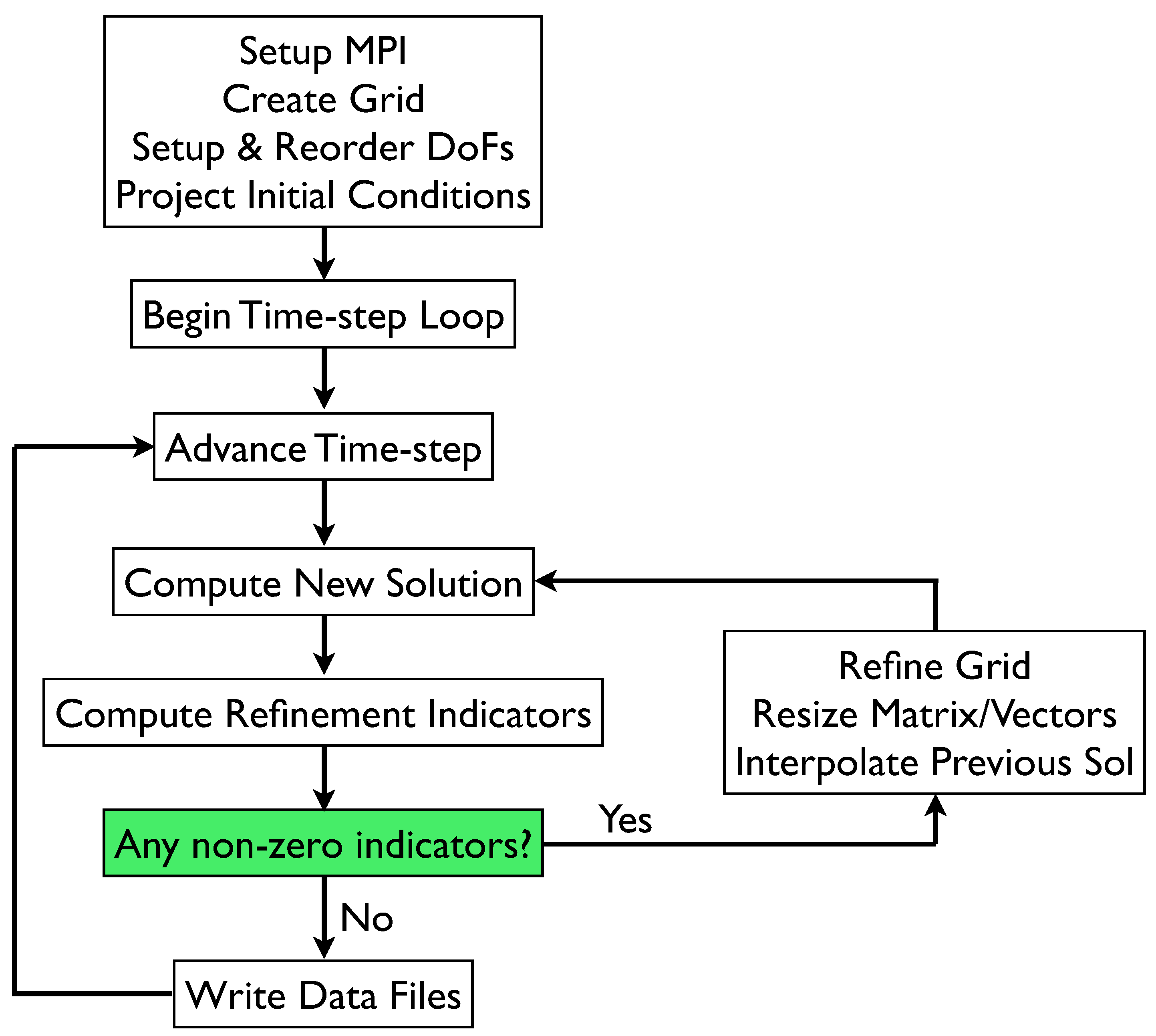
where c is a constant, $h_K$ is the diameter of the K-th cell and $h_{\text{min}}$ is the minimum cell diameter allowed in the simulation. The use of a minimum mesh size is a simple and well-known method for addressing localization. Here we propose that it should be related to the particular microstructure of the body in question; however, we provide no relationship between $h_{\text{min}}$ and any specific physics, as the point of this paper is not the physical model itself but rather numerical techniques. The constant c in (39) allows us to adjust the excess energy release rate. In particular, $c<1$ will cause $r_K^G$ to be non-zero before damage growth occurs, and in effect preemptively refine the mesh. The complete mesh refinement algorithms are given in Figure 1 and Figure 2, for the damage based scheme and the energy release rate scheme, respectively. The minimum cell length defines the scale at which damage evolution will occur. Accordingly, each of the algorithms iterates through refinement cycles, within a given timestep, until each cell which has a non-zero refinement indicator has a diameter less than $h_{\text{min}}$. No mesh coarsening is implemented, as we do not want to have damage evolving at a mesh size greater than the minimum one.

Throughout the refinement process, the triangulation is changed, resulting in the need to resize the associated matrices and vectors, as well as transfer the solution from the previous triangulation to the new one. This require time and changing memory requirements, and are detrimental to the performance of the code. However, even with these performance issues, the resulting algorithm is still much faster than using a fine scale mesh from the onset of the simulation.

Figure 1. Damage based refinement algorithm flow chart.

Figure 1. Damage based refinement algorithm flow chart.

Figure 2. Energy Release Rate based algorithm flow chart.

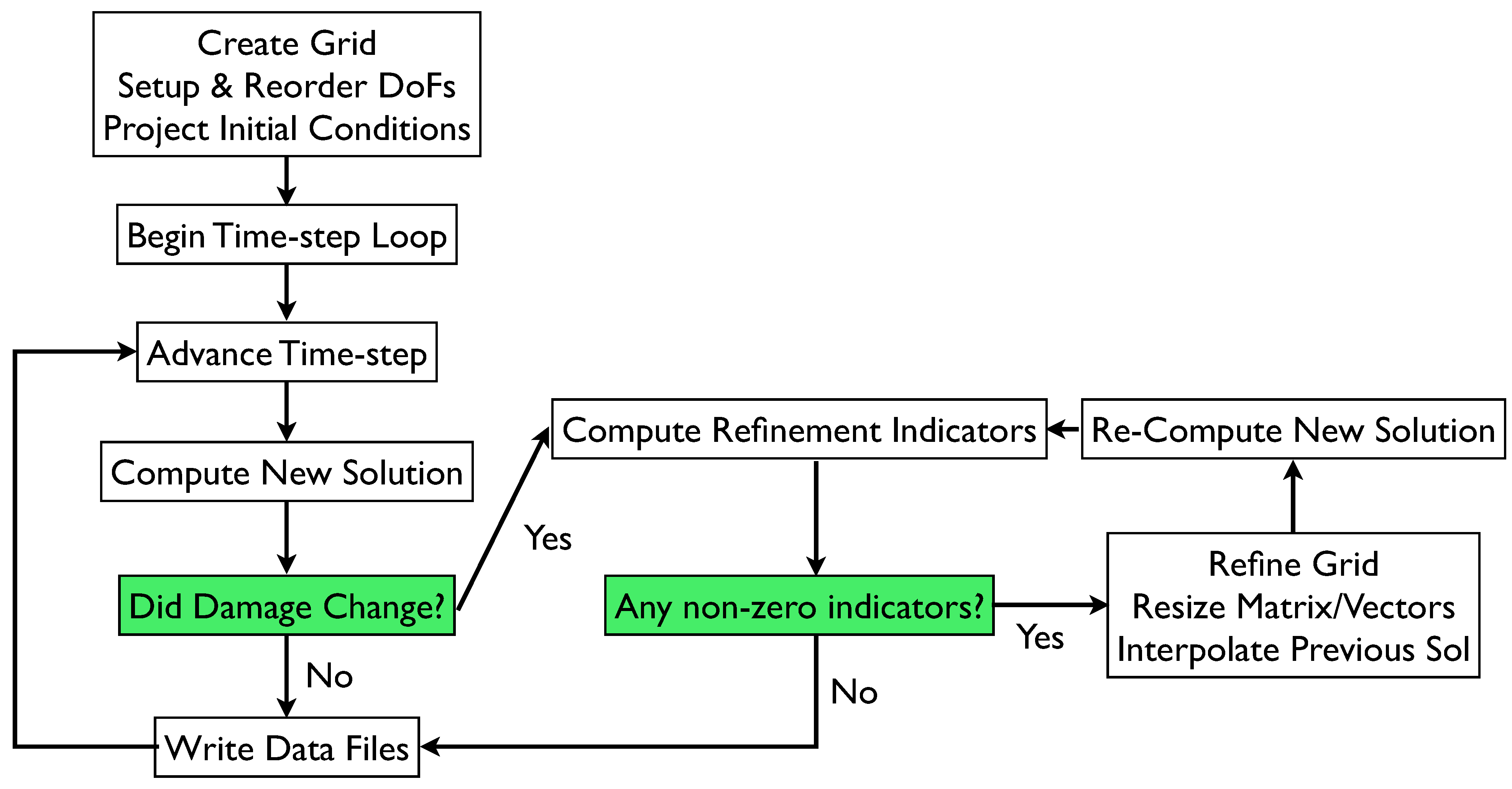
Figure 2. Energy Release Rate based algorithm flow chart.

5. Numerical Experiments

In this section we investigate the performance of the proposed algorithms. A simple example consisting of a two-dimensional bar fixed at one end and subjected to an applied load at the other is used to gain confidence that the proposed algorithms are functioning as desired. A more complicated example, consisting of a two-dimensional idealization of a compact test specimen is used to evaluate how well the algorithms address the use of different meshes, by visually comparing the resulting damage fields on each triangulation.

The geometry of a two-dimensional bar fixed at one end and subjected to a Neumann (traction) boundary condition at the other is given in Figure 3.

Figure 3. Geometry and boundary conditions of a two-dimensional bar fixed at $X_1=0$ and subject to an applied traction at $X_1=L$.

Figure 3. Geometry and boundary conditions of a two-dimensional bar fixed at $X_1=0$ and subject to an applied traction at $X_1=L$.

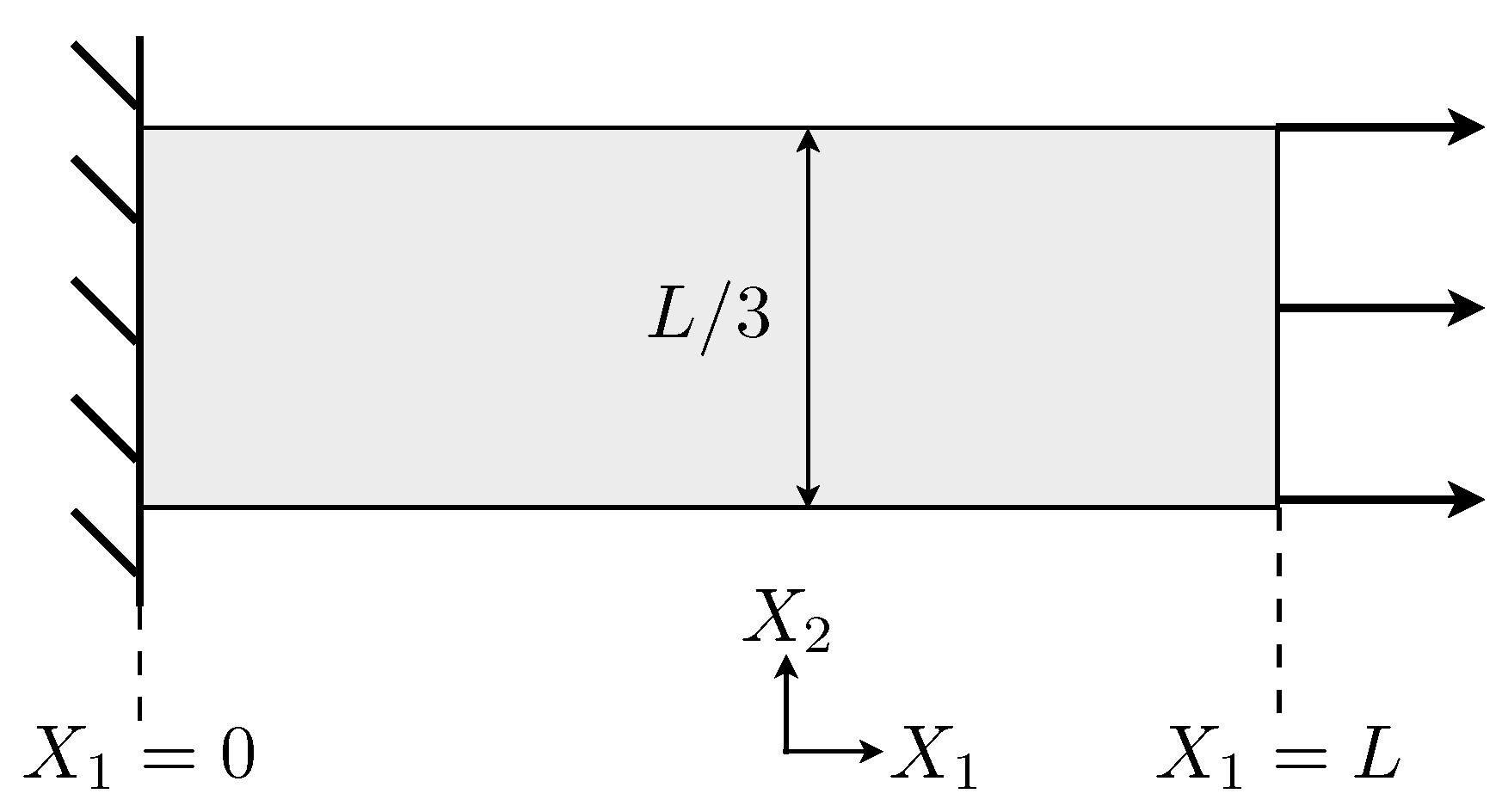
The essential boundary conditions are ${\mathbf{u}|}_{X_1=0}=\mathbf{0}$ and ${\mathbf{v}|}_{X_1=0}=\mathbf{0}$, and the applied traction force is defined as the smooth function

$${\mathbf{s}}_{\kappa }{(X,t)|}_{X_1=L}=\left\{\begin{array}{cc}\frac{{\mathbf{s}}_0}{2}\left(1-cos\frac{2\pi t}{\tau }\right)\hfill & t<\frac{\tau }{2}\hfill \\ {\mathbf{s}}_0\hfill & t\ge \frac{\tau }{2}\hfill \end{array}\right.,$$

(40)

where ${\mathbf{s}}_0={[s_x,0]}^T$. The initial conditions are $\mathbf{u}(X,t)=\mathbf{0}$, $\mathbf{v}(X,t)=\mathbf{0}$, and $\varphi (X,t)=0.001$. This simple initial boundary value problem corresponds to a two-dimensional bar which is clamped at one end, and initially at rest with uniform damage, being smoothly loaded up to a particular load at which time the load is held constant. Thus, a wave will propagate along the bar, eventually striking the fixed end. The particular material properties and parameters for the following simulations are given in Table 1, and have been chosen to be representative of a brittle material.

Table 1. Material properties representative of a brittle material, and the loading parameters.

Elastic Modulus	9 ×109 Pa	Density	1.7 × 103 kg/m3
Poisson Ratio	0.3	Gcr	3 × 107 J/m3
ηc	0.1 m3/J·s	β	2
τ	20 μs	sx	5× 107 Pa

Table 1. Material properties representative of a brittle material, and the loading parameters.

Elastic Modulus	9 ×109 Pa	Density	1.7 × 103 kg/m3
Poisson Ratio	0.3	Gcr	3 × 107 J/m3
ηc	0.1 m3/J·s	β	2
τ	20 μs	sx	5× 107 Pa

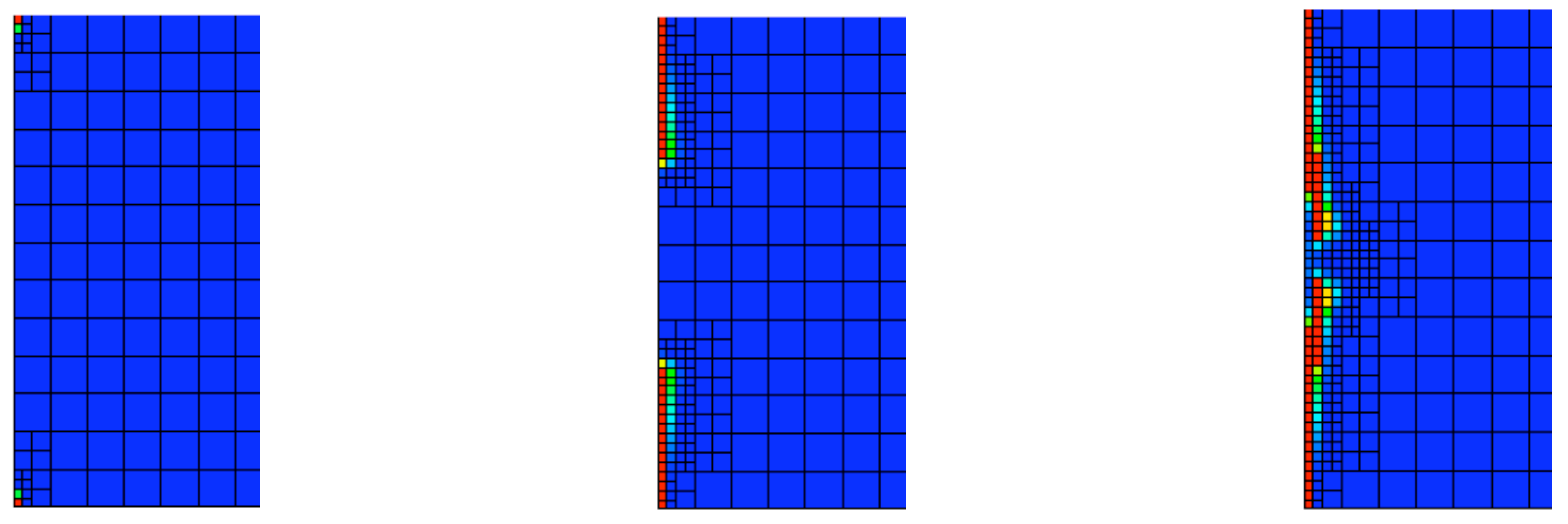
Figure 4. Damage-based refinement scheme: from top to bottom, triangulations of the two-dimensional bar at times $t=0$, $t=$88.5 μs, $t=$ 106.1 μs, and $t=$ 115.9 μs. The refinement is concentrated at the fixed end of the bar, which is where we expect the damage to increase.

Figure 4. Damage-based refinement scheme: from top to bottom, triangulations of the two-dimensional bar at times $t=0$, $t=$88.5 μs, $t=$ 106.1 μs, and $t=$ 115.9 μs. The refinement is concentrated at the fixed end of the bar, which is where we expect the damage to increase.

We see in Figure 4 that the mesh refinement is localized to the fixed (left) end of the bar, indicating that this is where the damage is increasing. This is expected, because as the wave strikes the fixed end of the bar, we expect from the theory of linear elasticity to have very high strains at the corners of the domain, and thus an energy release rate that is higher than other locations in the domain. We plot the values of the damage variable in Figure 5, and see that the damage nucleates at the corners of the domain, and subsequently, as the corner cells become fully damaged we see the adjacent cell become damaged, and so on. The damage-based refinement scheme only allows for damage evolution at the smallest mesh size. We can see this in Figure 5, where the piecewise constant damage is clearly localized to an individual cell at the smallest refinement level. We see that there is no damage evolution in larger cells, as desired. We now want to compare the performance of the damage based and energy release rate based error estimation schemes.

Figure 5. Damage based refinement: from left to right, zoom-in images of the damage at the fixed-end of the bar $X=0$, at $t=$88.5 μs, $t=$ 106.1 μs, and $t=$ 115.9 μs. The damage nucleates at the corners of the bar, and progresses towards the center.

Figure 5. Damage based refinement: from left to right, zoom-in images of the damage at the fixed-end of the bar $X=0$, at $t=$88.5 μs, $t=$ 106.1 μs, and $t=$ 115.9 μs. The damage nucleates at the corners of the bar, and progresses towards the center.

Figure 6. Energy release rate based refinement, with $c=1$: from left to right, zoom-in images of the damage at the fixed-end of the bar $X=0$, at $t=$88.5 μs, $t=$ 106.1 μs, and $t=$ 115.9 μs.

Figure 6. Energy release rate based refinement, with $c=1$: from left to right, zoom-in images of the damage at the fixed-end of the bar $X=0$, at $t=$88.5 μs, $t=$ 106.1 μs, and $t=$ 115.9 μs.

Figure 7. Energy release rate based refinement, $c=0.5$: The same simulation as in Figure 6, but now with the refinement indicator parameter $c=0.5$. Note the difference in the mesh pattern, specifically the refinement of cells in which damage is not evolving.

Figure 7. Energy release rate based refinement, $c=0.5$: The same simulation as in Figure 6, but now with the refinement indicator parameter $c=0.5$. Note the difference in the mesh pattern, specifically the refinement of cells in which damage is not evolving.

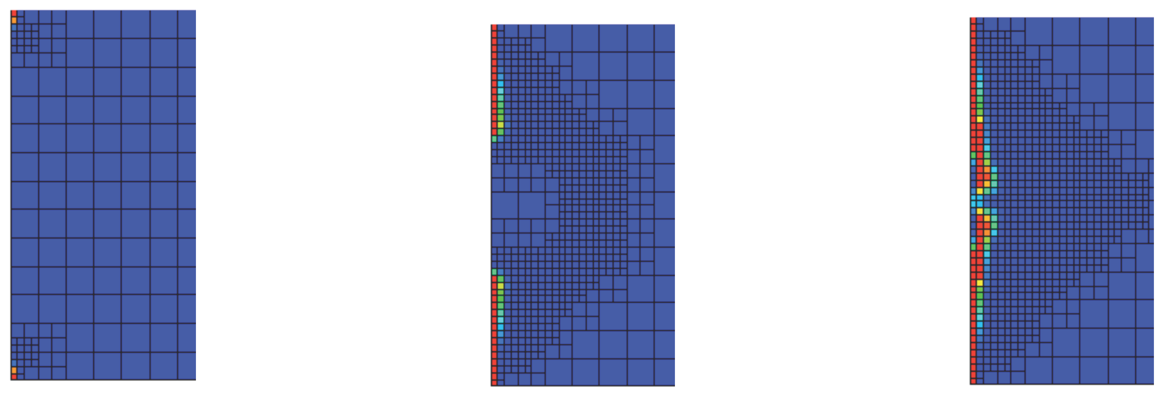
Figure 8. The first principle stress versus the first principle strain at a point which becomes fully damaged (left) and the corresponding time series of the damage variable and Helmholtz free energy density (right). Dynamic effects can be observed in both data sets. On the right, region I corresponds to the response before damage evolution, region II to the brief period of damage evolution, and region III to the period when the material is fully damaged.

Figure 8. The first principle stress versus the first principle strain at a point which becomes fully damaged (left) and the corresponding time series of the damage variable and Helmholtz free energy density (right). Dynamic effects can be observed in both data sets. On the right, region I corresponds to the response before damage evolution, region II to the brief period of damage evolution, and region III to the period when the material is fully damaged.

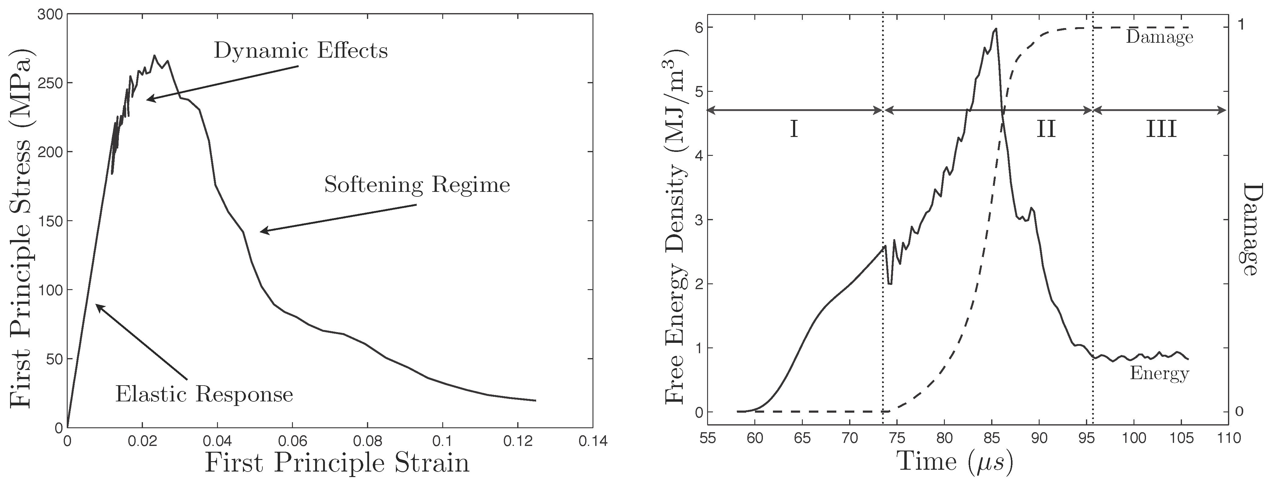
To serve as a check that the simple damage model we have chosen to use for demonstration purposes is functioning correctly, in Figure 8 we provide a plot of the first principle stress versus the first principle strain at a point which becomes fully damaged (left) and the corresponding time series of the damage variable and Helmholtz free energy density (right). The point we have chosen is the center of the bottom left cell in Figure 7. Note that both the parametric (in time) stress/strain plot and time series plot of the damage and energy are simply records of the motion of a point which becomes fully damaged, and are not comparable to the usual uniaxial stress strain curves.

Figure 6 shows the damage solution of the same problem, but now using the refinement indicators based on the excess energy release rate with the parameter c in (39) set equal to one. We observe that the damage solution in Figure 6, while not identical to that in Figure 5, is quite similar to it. We attribute the similarity in the damage solutions to the fact that we have set $c=1$ in (39), and hence the energy release rate refinement indicator is the same as the damage based indicator and produces similar results. To illustrate the effect of adjusting the constant c, in Figure 7 we show the damage solution and mesh refinement for the same problem, but this time obtained using an energy release based refinement indicator with the parameter $c=0.5$. Preemptive mesh refinement is now clearly visible in Figure 7, however, the damage field is still essentially the same as in Figure 5 and Figure 6. Thus, in this circumstance, it appears that either the damage based or energy release rate based schemes would provide adequate performance.

5.1. Idealized Compact Test Specimen

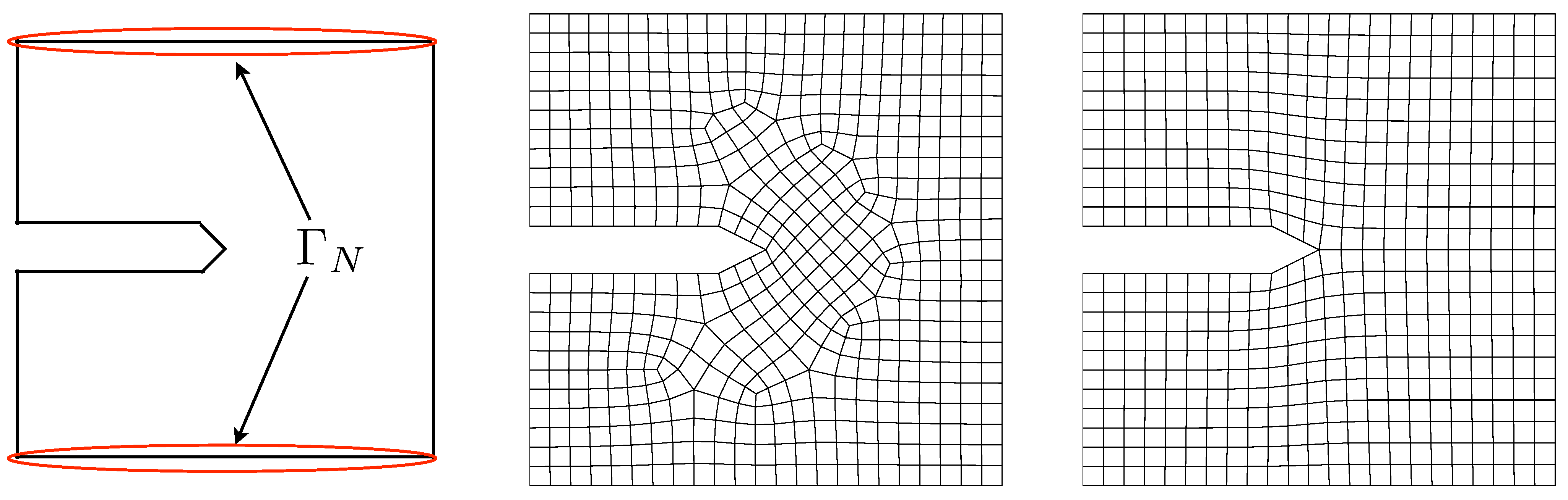
To further test and demonstrate the capabilities of the proposed algorithm, we choose to model the well known experiment of a compact test specimen in tension, in order to simulate conditions under which Mode I failure would normally occur. However, unlike many experiments of this nature, the loading on the specimen is monotonic and highly dynamic (as opposed to standard fatigue tests with slow, cyclic loading). The geometry and initial meshes for the simulations are given in Figure 9, and the boundary conditions are

$$\begin{array}{cccc}\hfill {\mathbf{s}}_{\kappa }(X,t)& =0\hfill & & X\in \partial {\mathcal{B}}_{\kappa }\backslash {\Gamma }_N\hfill \end{array}$$

(41)

$$\begin{array}{cccc}\hfill {\mathbf{s}}_{\kappa }(X,t)& =\left\{\begin{array}{cc}\frac{{\mathbf{s}}_0}{2}\left(1-cos\frac{2\pi t}{\tau }\right)\hfill & t<\frac{\tau }{2}\hfill \\ {\mathbf{s}}_0\hfill & t\ge \frac{\tau }{2}\hfill \end{array}\right.\hfill & & X\in {\Gamma }_N,\hfill \end{array}$$

(42)

where ${\mathbf{s}}_0={[0,s_y]}^T$. The initial conditions are $\mathbf{u}(X,t)=\mathbf{0}$, $\mathbf{v}(X,t)=\mathbf{0}$, and $\varphi (X,t)=0.001$, and the material properties are listed in Table 1, with the exception that now we take ${\eta }_c=0.05{\text{m}}^3/\text{J}·s$ and $G_{cr}=1\times {10}^7\text{J}/{\text{m}}^3$.

Figure 9. Geometry and initial meshes for the simulations of an idealized 2D compact test specimen. Vertical traction loading is applied to the faces denoted as ${\Gamma }_N$, creating a situation likely to result in Mode I failure. The meshes were created using the pave (left) and submap (right) methods in Cubit [17].

Figure 9. Geometry and initial meshes for the simulations of an idealized 2D compact test specimen. Vertical traction loading is applied to the faces denoted as ${\Gamma }_N$, creating a situation likely to result in Mode I failure. The meshes were created using the pave (left) and submap (right) methods in Cubit [17].

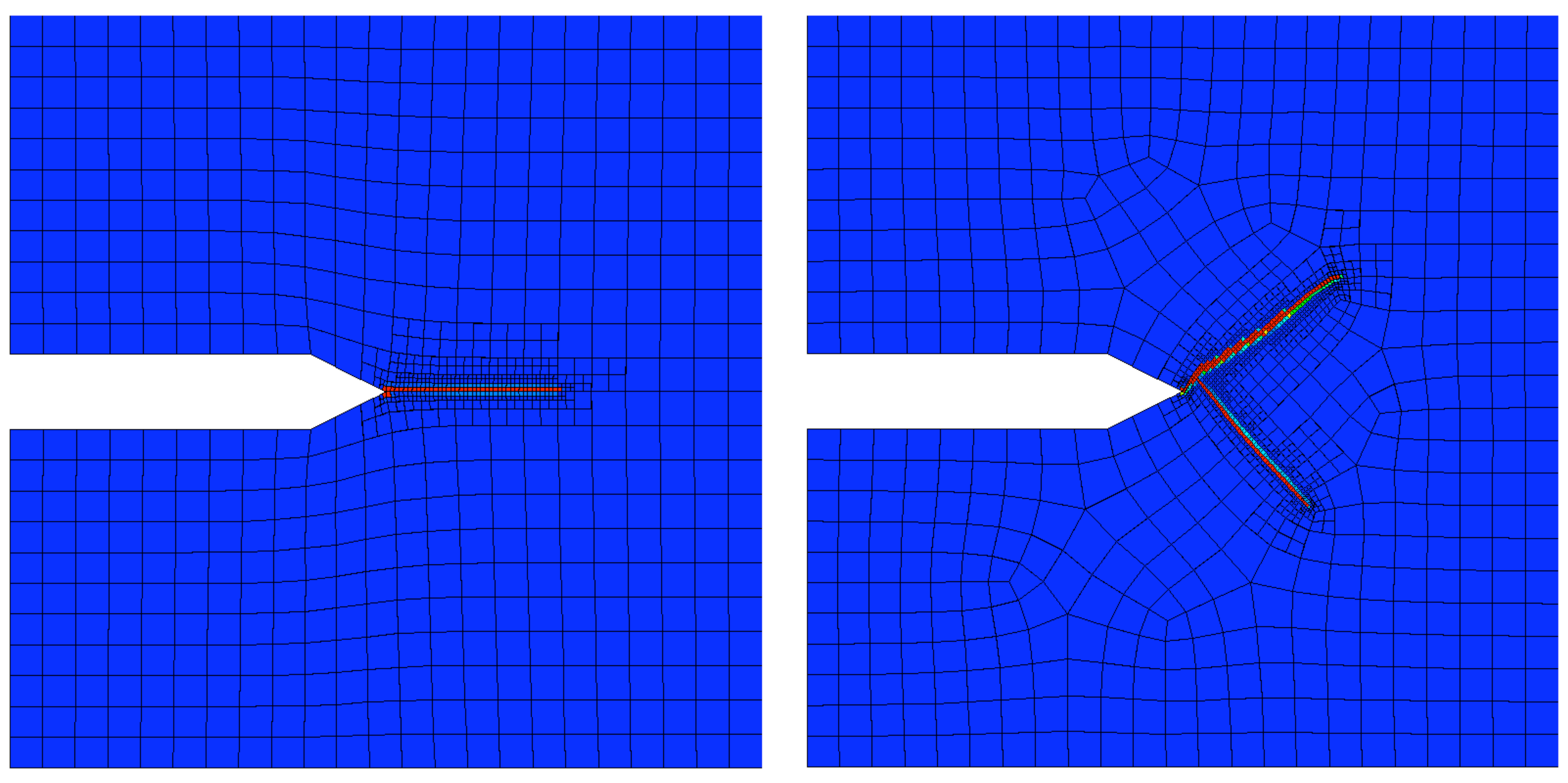
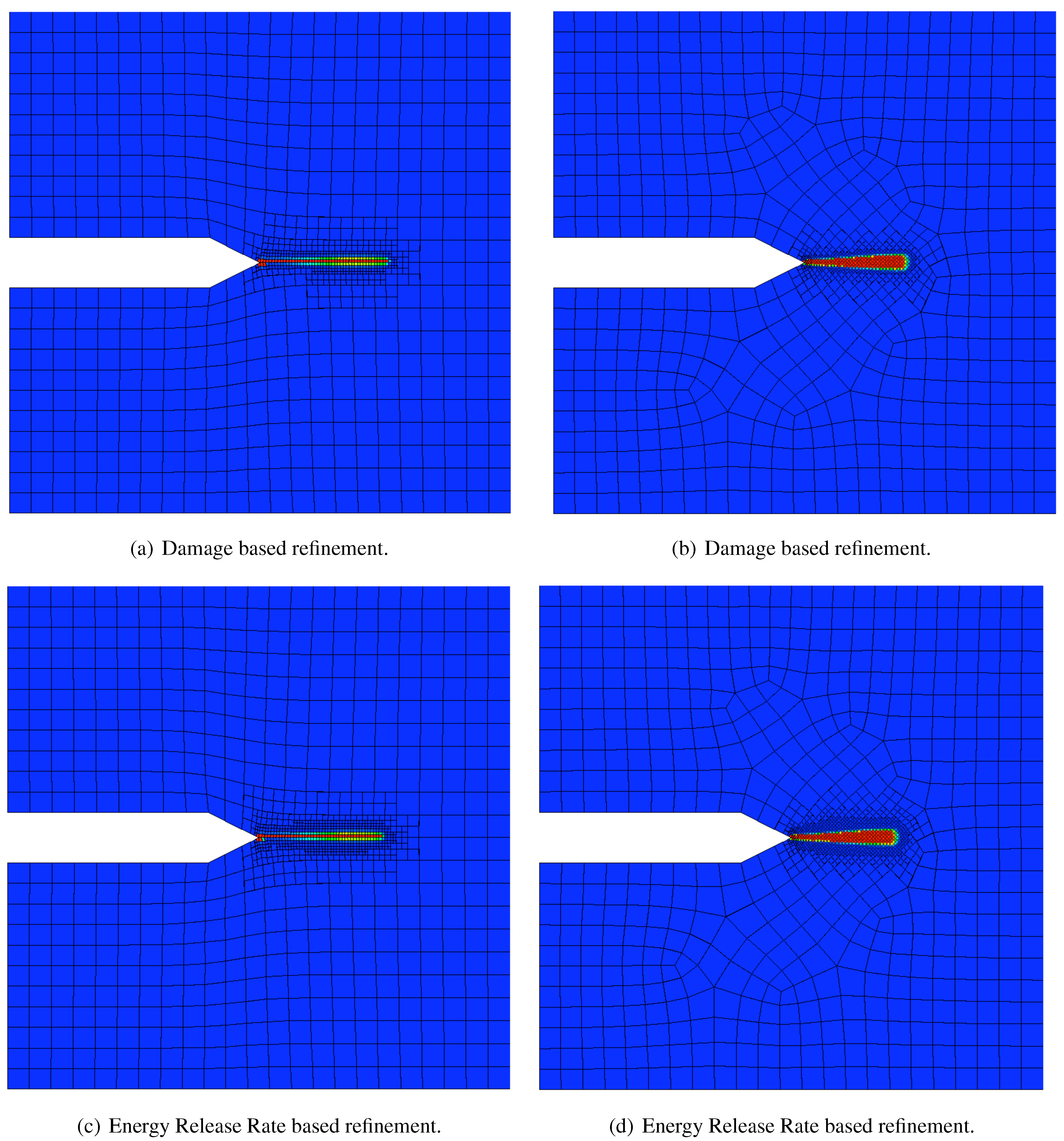
For this specific loading condition and set of material properties (including $h_{\text{min}}$), we see in Figure 10 that both the damage and energy release rate based refinement schemes show similar results for the damage solution on both initial meshes, thus demonstrating that the solution is somewhat independent of the mesh. By this we mean that, while the two damage distributions are clearly not identical, they do concentrate on the horizontal symmetry line of the compact specimen, as expected. As it turns out, the differences between the solutions obtained using different initial grids can be traced to the specific values used for the parameter $h_{\text{min}}$ in relation to that of the parameter $G_{cr}$. Before addressing this issue, we remark that for the results shown in Figure 10, the parameter in the energy release rate based refinement algorithm is $c=0.5$, and as such, we notice that the corresponding solutions in Figure 10(c) and Figure 10(d) have a slightly greater extent of refinement. However, comparing the damage solutions in Figure 10(a) and Figure 10(b) with those in Figure 10(c) and Figure 10(d), we see that the preemptive refinement of the energy release rate based algorithm yielded essentially the same damage solution as that produced by the refinement indicator based on the time rate of change of the damage. Therefore, we conclude again that in this instance, either scheme is adequate.

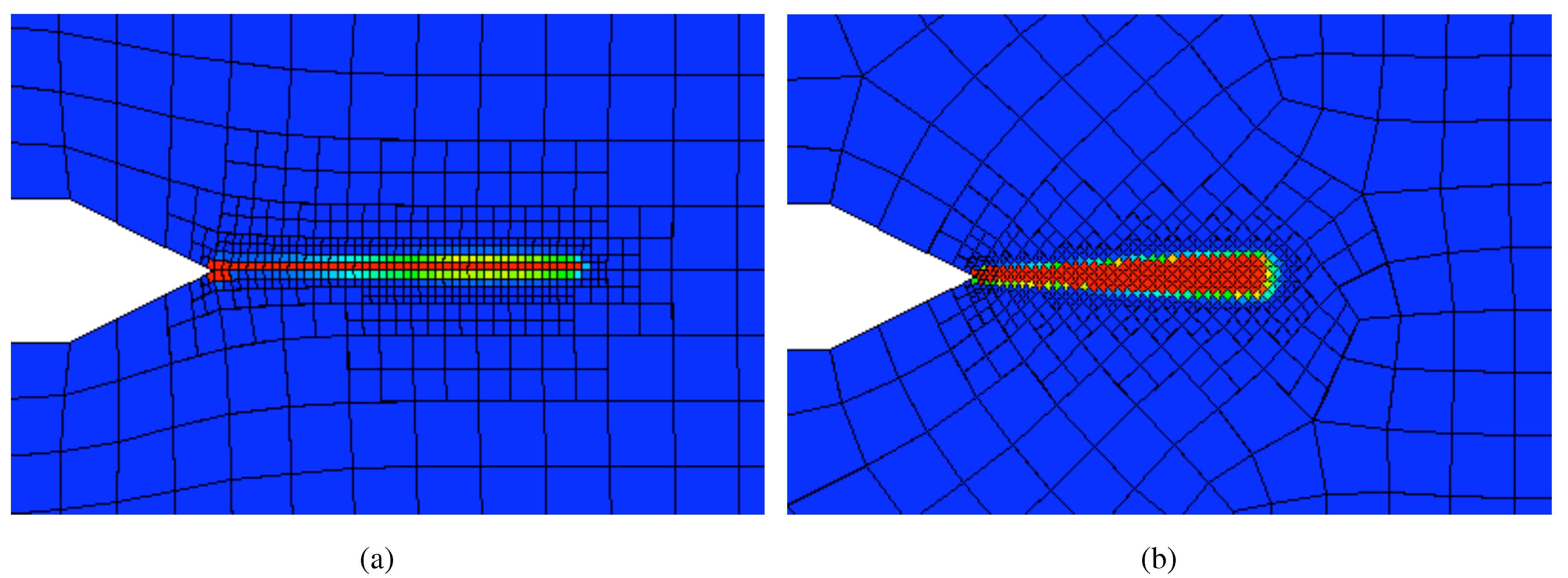
Going back to discussing the mesh dependence issue, the most noticeable difference between the solutions on the grid in Figure 10(a) and Figure 10(c) and the grid in Figure 10(b) and Figure 10(d) is the degree of localization of the damage solution. In the first set of aforementioned figures, the damage is localized to a single cell, while in the second set the damage is clearly spread over numerous cells across the horizontal mid-line of the solution domain. Figure 11(a) and Figure 11(b) show the region of interest in Figure 10(a) and Figure 10(b), respectively. It is clear in these figures that, with the choice of piecewise constant elements, the damage solution seems to evolve in cells that are adjacent to the face of an already damaged cell, as opposed to one which is connected only at a corner. We discovered that this effect becomes more pronounced as we increase the value of $G_{cr}$ while keeping the value of $h_{\text{min}}$ fixed.

In fact, taking the value of $G_{cr}=3\times {10}^7\text{J}/{\text{m}}^3$, which is three times the value used to produce the solutions in Figure 10(a)–Figure 10(d), we see in Figure 12 that the ability of the algorithm to address the mesh-dependency of the solution is diminished (again, keeping in mind that the value of $h_{\text{min}}$ is held constant) to the point that two completely different physical failure patters are obtained. We suspect that to obtain physically comparable solutions on different initial meshes, we would need to determine the influence the values of $h_{\text{min}}$ and $G_{cr}$ have on each other. However, this may not be an acceptable solution due to the fact that the value used for $h_{\text{min}}$ should be physical-based, that is, as though $h_{\text{min}}$ were a constitutive parameter. Clearly this also means that comparing solutions with vastly different values of $G_{cr}$ while keeping $h_{\text{min}}$ fixed may be questionable. With this in mind, we feel that the results presented in this paper demonstrate that the proposed algorithm is well suited for locally refining the mesh in areas of evolving damage, but could certainly be more robust. Specifically, the authors feel that more careful study of the combination of solution space choices for the damage variable, error estimates, and refinement strategies are necessary before any more general claims can be made about the viability of using adaptive h-refinement for addressing mesh dependency of damage models prone to localization.

Figure 10. Damage solutions on two very different meshes with the two proposed refinement algorithms. In these simulations, the constant in (39) is $c=0.5$, leading to the preemptive refinement of non-damaged cells in Figure 10(c) and Figure 10(d). In general, the solutions are all similar, thus we are encouraged that adaptive mesh refinement may be able to help control mesh-dependency issues; however, it is clear that the extent of localization is different between the two meshes and not yet to a point of mathematical comparison.

Figure 10. Damage solutions on two very different meshes with the two proposed refinement algorithms. In these simulations, the constant in (39) is $c=0.5$, leading to the preemptive refinement of non-damaged cells in Figure 10(c) and Figure 10(d). In general, the solutions are all similar, thus we are encouraged that adaptive mesh refinement may be able to help control mesh-dependency issues; however, it is clear that the extent of localization is different between the two meshes and not yet to a point of mathematical comparison.

Figure 11. Zoom-in of the damage solutions in Figure 10(a) and Figure 10(b), respectively, showing the damage field solution produced by the damage-based refinement algorithm. The extent to which the damage is localized is clearly visible, and, for this first attempt, is considered thus far to be sucessful.

Figure 11. Zoom-in of the damage solutions in Figure 10(a) and Figure 10(b), respectively, showing the damage field solution produced by the damage-based refinement algorithm. The extent to which the damage is localized is clearly visible, and, for this first attempt, is considered thus far to be sucessful.

Figure 12. Damage field solutions using the energy release rate refinement algorithm, but with $G_{cr}$ three times larger than the value used to find the solutions in Figure 10(c)–Figure 10(d). Clearly, the ability of the algorithm to mitigate the mesh dependence is diminished.

Figure 12. Damage field solutions using the energy release rate refinement algorithm, but with $G_{cr}$ three times larger than the value used to find the solutions in Figure 10(c)–Figure 10(d). Clearly, the ability of the algorithm to mitigate the mesh dependence is diminished.

6. Summary

In this paper, a first attempt at employing adaptive mesh refinement to dynamic damage evolution in brittle materials is presented. In terms of effectively refining the mesh locally where damage is evolving, the algorithm works very well. Two original simple adaptive mesh refinement algorithms were derived and presented. Their ability to address the localization and mesh-dependency of the damage solution for the simple case of a linear elastic body with scalar damage was investigated. Under some circumstances the algorithms worked quite well; however, the proposed combination of a piecewise discontinuous solution space for the damage solution and the refinement algorithms is not universally successful.

Future exploration of appropriate solution spaces for the damage variable is necessary. The authors believe that discontinuous solution spaces should be employed, as they allow for a more flexible interpolation of damage fields with low regularity and tendency for localization. Additionally, the relation between the refinement indicators used and limiting minimum mesh size, as well as the other constitutive parameters controlling damage evolution needs to be studied more carefully to as to develop more robust strategies for solving localization prone systems without modifying the equations of motion.

References

- Mariano, P. Premises to a Multifield Approach to Stochastic Damage Evolution. In Damage and Fracture of Disordered Materials; Krajcinovic, D., van Mier, J., Eds.; Springer: Wien, Austria, 2000; Vol. 410, chapter 6; pp. 217–263. [Google Scholar]
- Peerlings, R.; de Borst, R.; Brekelmans, W.; de Vree, J. Gradient-enhanced damage for quasi-brittle materials. Int. J. Numer. Method. Eng. 1996, 39, 3391–3403. [Google Scholar] [CrossRef]
- Pijaudier-Cabot, G.; Bazant, Z. P. Non-local damage theory. J. Eng. Mech.—ASCE 1987, 113, 1512–1533. [Google Scholar] [CrossRef]
- Comi, C. A nonlocal model with tension and compression damage mechanisms. Eur. J. Mech. - A/Solids 2001, 20, 1–22. [Google Scholar] [CrossRef]
- Krajcinovic, D. Damage Mechanics; Elsevier Science: Maryland Heights, MO 63043, USA, 1996. [Google Scholar]
- Caiazzo, A.; Costanzo, F. On the constitutive relations of materials with evolving microstructure due to microcracking. Int. J. Solids Struct. 2000, 37, 3375–3398. [Google Scholar] [CrossRef]
- Coleman, B.; Gurtin, M. Thermodynamics with internal state variables. J. Chem. Physics 1967, 47, 597–613. [Google Scholar] [CrossRef]
- Bowen, R. M. Introduction to Continuum Mechanics for Engineers; Plenum Press: New York, NY, USA, 1989. [Google Scholar]
- Coleman, B.; Noll, W. The thermodynamics of elastic materials with heat conduction and viscosity. Archive for Rational Mechanics and Analysis 1963, 13, 167–178. [Google Scholar] [CrossRef]
- Gurtin, M. E. An Introduction to Continuum Mechanics; Academic Press: New York, USA, 1981. [Google Scholar]
- Arnold, D.; Brezzi, F.; Cockburn, B.; Marini, L. Unified analysis of discontinuous Galerkin methods for elliptic problems. SIAM J. Numer. Analysis 2002, 39, 1749–1779. [Google Scholar] [CrossRef]
- Simo, J. C.; Hughes, T. J. R. Computational Inelasticity; Springer-Verlag: New York, USA, 1998. [Google Scholar]
- Quarteroni, A.; Sacco, R.; Saleri, F. Numer. Math.; Springer-Verlag New York, Inc.: New York, NY, USA, 2000. [Google Scholar]
- Bangerth, W.; Hartmann, R.; Kanschat, G. deal.ii differential equation analysis library, technical reference. Technical report. Texas A&M University, 2006. [Google Scholar]
- Babuška, I.; Rheinboldt, W. C. A-Posteriori Error Estimates for the Finite Element Method. Int. J. Numer. Method. Eng. 1978, 12, 1597–1615. [Google Scholar] [CrossRef]
- Kelly, D. W.; De, J. P.; Gago, S. R.; Zienkiewicz, O. C.; Babuška, I. A-Posteriori Error Analysis and Adaptive Processes in the Finite Element Method: Part I—Error Analysis. Int. J. Numer. Method. Eng. 1983, 19, 1593–1619. [Google Scholar] [CrossRef]
- Sandia National Laboratories. Cubit Geometry and Mesh Generation Toolkit. Available online: http://cubit.sandia.gov.
- 1.The notation is standard in the field of partial differential equations to denote the Sobolev space of Lebesgue integrable functions whose weak derivatives of order one are also integrable. The notation denotes the space of square (Lebesgue) integrable functions. Although we have not explicitly indicated it, it is understood that the spaces in question conform to the prescribed Dirichlet boundary conditions for the fields of interest.
- 2.Ω is the domain of the problem.
- 3.This is typically the case in Discontinous Galerkin (DG) finite element methods (see, e.g., [11]).
- 4.Note that there is a distinction between error estimators and refinement indicators. The former measure the error present in the approximate solution for a given cell in the triangulation, while the latter simply determines whether or not the cell should be refined. While these two concepts are often used together, in this paper, we are simply interested in refining the mesh where damage is evolving without any direct attempt to estimate the error.
© 2009 by the authors; licensee MDPI, Basel, Switzerland. This article is an open access article distributed under the terms and conditions of the Creative Commons Attribution license (http://creativecommons.org/licenses/by/3.0/).
Share and Cite
MDPI and ACS Style
Pitt, J.S.; Costanzo, F. An Adaptive h-Refinement Algorithm for Local Damage Models. Algorithms 2009, 2, 1281-1300. https://doi.org/10.3390/a2041281
AMA Style
Pitt JS, Costanzo F. An Adaptive h-Refinement Algorithm for Local Damage Models. Algorithms. 2009; 2(4):1281-1300. https://doi.org/10.3390/a2041281
Chicago/Turabian StylePitt, Jonathan S., and Francesco Costanzo. 2009. "An Adaptive h-Refinement Algorithm for Local Damage Models" Algorithms 2, no. 4: 1281-1300. https://doi.org/10.3390/a2041281