Methodology, Algorithms, and Emerging Tool for Automated Design of Intelligent Integrated Multi-Sensor Systems

Abstract

The emergence of novel sensing elements, computing nodes, wireless communication and integration technology provides unprecedented possibilities for the design and application of intelligent systems. Each new application system must be designed from scratch, employing sophisticated methods ranging from conventional signal processing to computational intelligence. Currently, a significant part of this overall algorithmic chain of the computational system model still has to be assembled manually by experienced designers in a time and labor consuming process. In this research work, this challenge is picked up and a methodology and algorithms for automated design of intelligent integrated and resource-aware multi-sensor systems employing multi-objective evolutionary computation are introduced. The proposed methodology tackles the challenge of rapid-prototyping of such systems under realization constraints and, additionally, includes features of system instance specific self-correction for sustained operation of a large volume and in a dynamically changing environment. The extension of these concepts to the reconfigurable hardware platform renders so called self-x sensor systems, which stands, e.g., for self-monitoring, -calibrating, -trimming, and -repairing/-healing systems. Selected experimental results prove the applicability and effectiveness of our proposed methodology and emerging tool. By our approach, competitive results were achieved with regard to classification accuracy, flexibility, and design speed under additional design constraints.

1. Introduction

Intelligent integrated multi-sensor systems are finding a more and more widespread range of applications in areas including the automotive, aerospace and defense industries, industrial, medical, building automation and security uses, and intelligent house and wear. This remarkable increase of applications is due to the ongoing advances in sensor and integration technology [1,2,3,4], computing nodes [5,6], wireless communication [7,8,9], and signal processing algorithms [10,11,12,13]. Such intelligent multi-sensor systems also require, however, a larger variety of sensor electronics and sensor signal processing techniques to be efficiently employed in all these different applications.

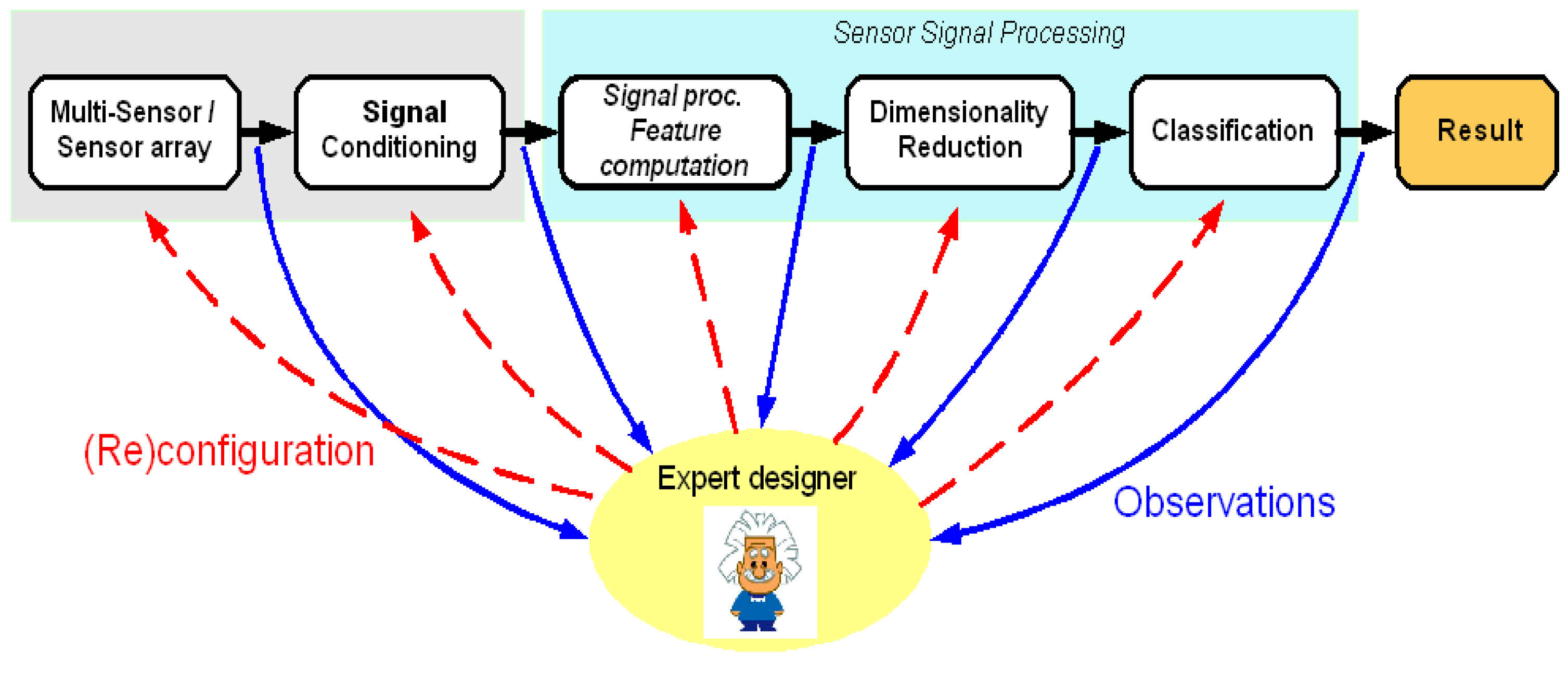
Currently, a significant part of intelligent sensor systems are still manually created by more or less experienced designers and need to be adapted or reengineered for each new application or different task. The design process goes through the main steps of sensor selection and scene optimization, analog and digital hardware selection or conception, choice of signal and feature processing, dimensionality reduction, and classification. Although the sensor selection, sensor parameter selection and the processing steps of dimensionality reduction and classification are more and more the subject of automation efforts, employing learning and optimization techniques [14,15,16], the decisive tasks of selection, combination, and parameter setting of heuristic signal processing and feature computation method are currently left to the human designers as a tedious, time and labor consuming task with potentially suboptimal outcome. In particular, the great diversity of available methods and tools from conventional signal processing to computational intelligence techniques imposes severe challenges on the experience and qualifications of the designer. Similar problems have already inspired research and implementation in the field of industrial vision and the design of corresponding image processing systems in the last fifteen years [61,62]. However, image processing and general sensor signal processing show substantial differences due to underlying physical principles. Thus, only inspirations from this work can be abstracted to our field of work and numerous extensions and modifications reflected by our research goals are required.

In numerous cases, the utilization of a single sensor is insufficient for deriving important information about particular measured objects. Other research activities have shown the need for multi-sensors or sensor arrays, e.g., in chemical sensing applications, for improving of the decision-making or the overall system performance [2,17]. However, these multi–sensor systems will increase the problem complexity and load on the designer for choosing and combining the proper signal processing and feature computation operators and the setting of the best parameters.

In a general approach for intelligent decision making task, e.g., airbag triggering in cars under the constraint of seat occupancy, the sensor signals are computed by operators of feature computation to extract the important features employed in a classifier unit for the recognition task. The features extracted from multi-sensor signals by feature computation operators enrich the dimensionality of data, which as a result increases the computational effort and could decrease the performance of a classifier due to the curse of dimensionality [18]. Therefore, some form of dimensionality reduction is usually applied to reduce the feature space of the data. One of the common dimensionality reduction methods, i.e., feature selection, has been applied in the optimization of intelligent sensor system design in order to reduce the cost measurement of overall system with eliminating the unimportant sensors and feature computation operators [19]. The feature computation and classifier selection, as well as the corresponding parameterization are crucial steps in the design process of intelligent multi–sensor systems.

In many optimization approaches for classification tasks, an objective or fitness function is mostly computed based on only the classification results. In our design approach, the multi–objective function is used based on the classification accuracy [20], overlap and compactness measurement of data structure [16] along with the constraints, i.e., the computational effort of feature computation and the number of selected feature [19]. In the context of our application domain, there are two commonly applied approaches of multi-objective optimization that have been proposed to solve the multi–objective problems, i.e., the aggregating method and Pareto–optimal methods [21]. In this paper, the aggregating method is adopted for this engineering problem for reasons of feasibility and complexity. More advanced schemes can be studied in the later stages of the work. For optimizing sensor selection, the combination and parameterization of feature computation, feature selection, and classifier, evolutionary computation (EC) techniques, in particular Genetic Algorithms (GA) [22,23] and Particle Swarm Optimization (PSO) [24,25] have been chosen. Both GA and PSO have been applied to optimize a variety of signal processing and feature computation as well as classification problems [12,19,20,26]. However, most of these prior approaches aim at optimizing only a single operator, without regard for the the overall system design.

Furthermore, according to predictions of technology roadmaps, mobile sensor nodes are expected to become constantly smaller and cheaper [27], potentially offering fast computation, constrained only by limited energy resources. This means that a designer has to achieve an efficient constrained design, i.e., select the combination of data processing techniques, which give low computation effort and only require small memory, but still perform well. This and a couple of other features, distinguish general sensor systems clearly from the field of industrial vision, where also several design automation or learning system designs can be observed [44,45]. These can provide some inspiration, but are not sufficient for the challenges in the general sensor system field.

Some research activities which have proposed methods and contributed to the activities for automated design of intelligent sensor systems, are briefly discussed in [28,29,30]. In [28], the authors focused on the sensor parameter selection for a multi-sensor array using genetic algorithms. In [29], a method to assist the designer of a sensor system in finding the optimal set of sensors for a given measurement problem was proposed. In [30], the authors proposed an algorithm based on particle swarm optimization (PSO) of model selection. This algorithm is capable of designing the best recognition system by finding a combination of pre-processing methods, feature selection, and learning algorithms from a given method pool, which provides the best recognition performance. The approach of Escalante et al. [30] does not try to optimize the selected standard models, e.g., nearest-neighbour classifier and probability neural network, with regard to resource awareness.

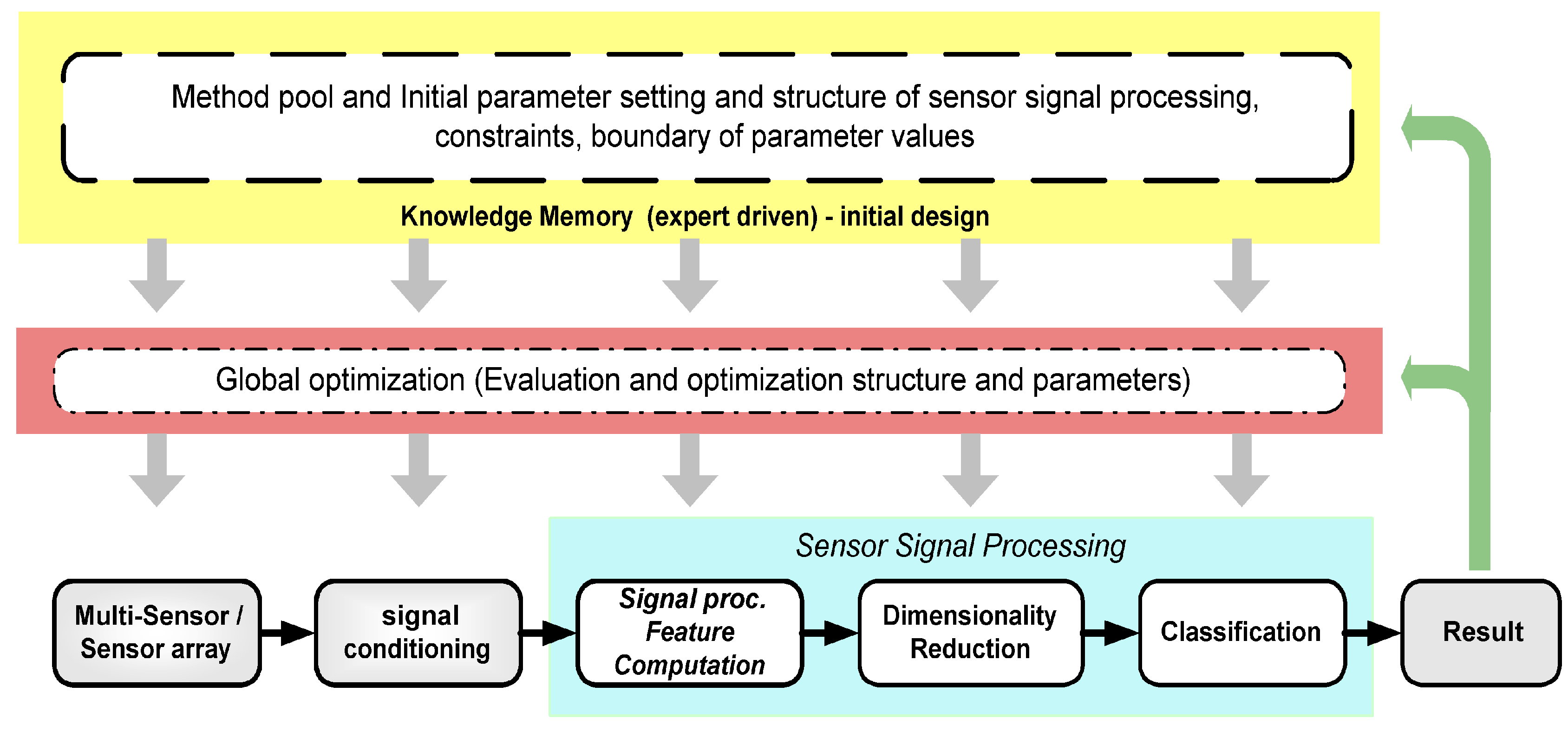
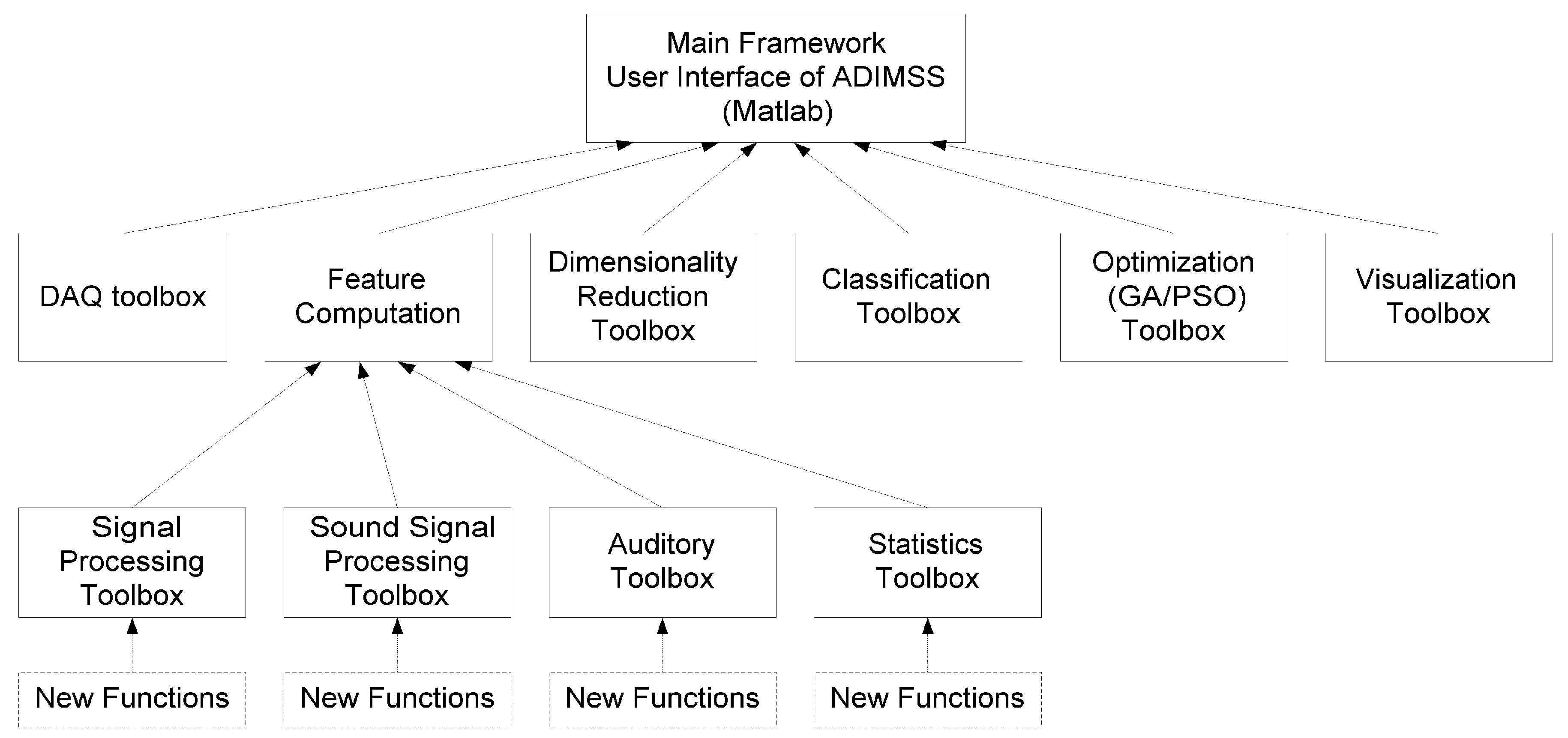
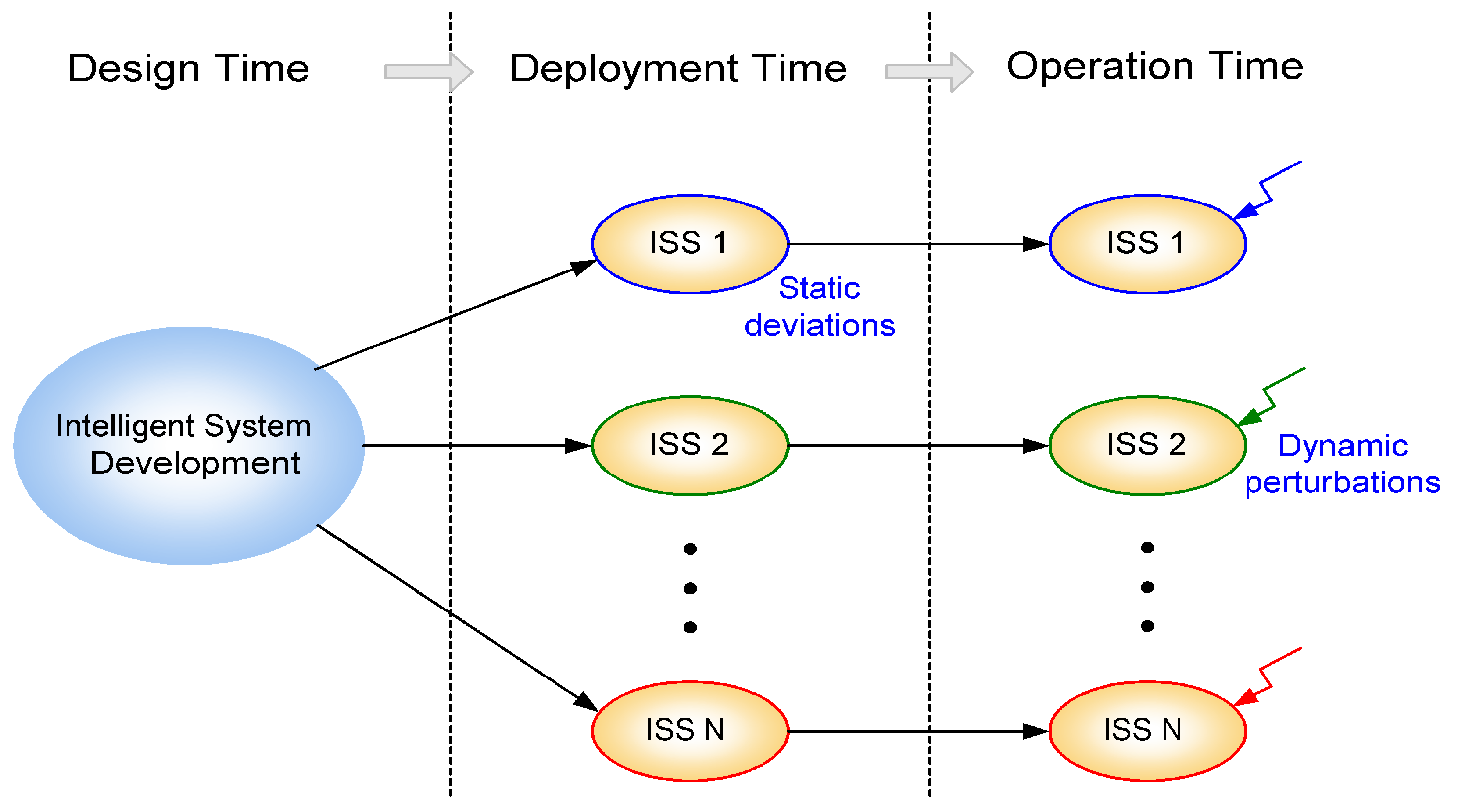
Our goals are to contribute to the automation of intelligent sensor systems that efficiently employ a rich and increasing variety of sensor principles and electronics for an increasing number of technical fields and tasks at feasible cost. For this purpose, we propose a concept, methodology, and a framework for automated design of intelligent multi-sensor systems (ADIMSS) based on well established as well as newly evolved signal processing and computational intelligence operators to build an application-specifc system. The proposed methodology is converted to a constantly growing toolbox based on Matlab. Our ADIMSS approach provides both rapid-prototyping properties, as well as adaptation or reconfiguration properties required when facing the deployment of the designed system to a larger volume of hardware instances, i.e., sensors and electronics, as well as the time-dependent influence of environmental changes and aging. The aim of our emerging tool is to provide flexible and computational effective solutions, rapid-prototyping under constraints, and robustness and fault tolerance at low effort, cost, and short design time. Such self-x features, e.g., for self-monitoring, -calibrating, -trimming, and -repairing/-healing systems [60], can be achieved at various levels of abstraction, from system and algorithm adaptation down to self-x sensor and system electronics. Our proposed architecture for intelligent sensor systems design can be applied in a broad variety of fields. Currently, we are focusing on ambient intelligence, home automation, MEMS (Micro Electromechanical Systems) based measurement systems, wireless–sensor–networks, and automotive applications.

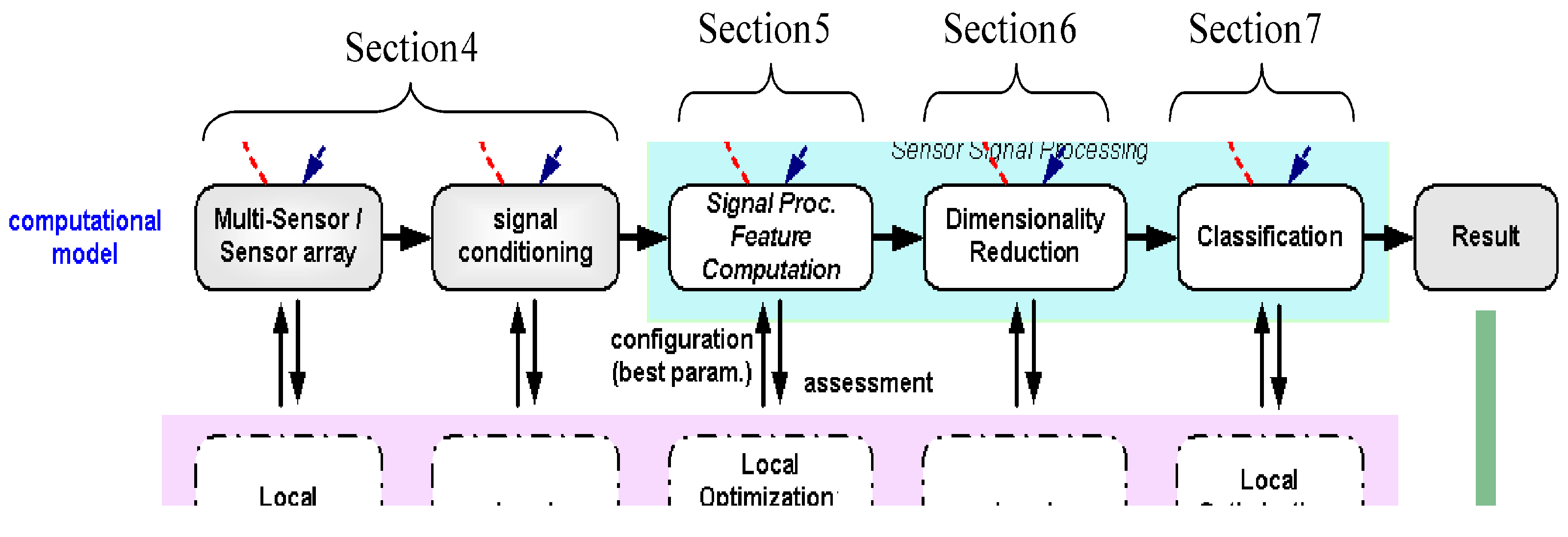
The next section will describe the conceived methodology of self-x intelligent sensor systems. In Section 3 we summarize aspects of evolutionary computation relevant for our particular work, focusing on genetic algorithm and particle swarm optimisation. Section 4 discusses approaches to design and optimise physical aspects of the sensor front-end. Section 5 treats options for systematically optimising sensor signal processing and feature computation methods. Section 6 regards available dimensionality reduction techniques and introduces in this context crucial issues of solution stability. Section 7 extends the employed optimisation and assessment methods to the classification task. Hardware constraints and resource awareness are treated for the example of a particular low power classifier implementation. For the aim of step by step demonstration of our approach, data of gas sensor systems or electronic nose and other benchmark datasets are applied to demonstrate the proposed method of sensor systems design (the approach has also been applied to industrial tasks and data, but publication permission is currently not granted).

2. Concepts and Architecture of Multi-Sensor Signal Processing

Intelligent sensor systems for potentially complex recognition tasks are composed of involved methods and algorithms with numerous parameters. Figure 1 exemplifies the standard building blocks of intelligent multi–sensor systems related to recognition applications. Of course, the graph shown simplifies the actual system, as more complex structures can be employed, e.g., for hierarchical classification or sensor fusion concepts. The tedious task of selecting, combining, and parameterizing methods of a method pool or even conceiving/developing new algorithms, is commonly burdened on a human designer. Such a manual, human–centered design process naturally consumes substantial human effort, time, and cost. Depending on the particular designer’s expertise, the manual approach can still deliver mediocre results. To alleviate the required effort and to achieve competitive results, design automation activities emerged as in other disciplines, e.g., chip design. Thus, in our work we pursue a shift of paradigm from expert-driven to automated design. In the following, we will outline the concept and describe our methodology, including the emerging ADIMSS tool based on evolutionary computation for constrained optimized design of intelligent sensor systems. The following subsections will discuss how the human expert can be effectively replaced by automation, similar to the development in other domains, e.g., microelectronics.

Figure 1. Block diagram of typical intelligent multi-sensor system. The design in each step or block depends human observation and assistance.

Figure 1. Block diagram of typical intelligent multi-sensor system. The design in each step or block depends human observation and assistance.

2.1. Global Optimization

Basically, in an automation approach, the human expert could be removed by a global optimization unit that is supported by a knowledge base, e.g., containing seed solutions and recommended parameter ranges and settings, for such search space reduction (see Figure 2). However, the concurrent optimization of the sensor selection, sensor parameters, and the chain of sensor signal processing methods will easily become infeasible for practical systems. As well-known, for instance, from feature selection, such exhaustive search approaches, though promising with regards to achievable solution quality, can only be applied to moderate search space dimensions. Thus, for reasons of tracktability and feasibility, a consecutive local optimization of subproblems is pursued and developed.

Figure 2. The concept of intelligent multi-sensor system design based on global optimization.

Figure 2. The concept of intelligent multi-sensor system design based on global optimization.

2.2. Local Optimization

The procedure of local optimization follows the divide-et-impera principle and dismantles the design problem into a set of local, smaller design problems with reduced search space, e.g., select or combine methods and to optimize their parameters, or structure gradually in the chain of sensor signal processing. However, the individual design steps depend on each other. This dependence can be honored, by letting the subproblems exhange information with their neighboring blocks. The simplest way to do this is to sequentially evolve the system. The direction of local optimization can be ‘bottom-up’ or ‘top-down’ optimization, as suggested by Figure 3. In this Figure, the top row repeats the general block strucuture of the intelligent multi-sensor system under design composed of multi-sensor/sensor array (including signal conditioning), signal pre-processing and enhancement, feature computation, dimensionality reduction, and classification (including the hierarchical classifiers). The second row illustrates the distributed optimization of the design tool, which in each local optimization block contains a potentially extensible collection of proven methods and algorithms of sensor and recognition systems and the local optimization tool, including single or multiple assessment methods from Section 3.5, for searching and finding of the best structure and parameters in each block. In addition to the the named assessment functions, which quantify the achieved decision making ability on the regarded level, further constraints related to, e.g., computational complexity and/or energy consumption, could be included as multiple objectives in the optimization approach on each level. As most the optimization tasks pursued here, rely on the concept of learning-from-examples, data and supervised information must be made available in an appropriate form on that level. This includes also statistically meaningful validation techniques employed in the design hierarchy.

Figure 3. The concept of intelligent multi-sensor system design based on local optimization.

Figure 3. The concept of intelligent multi-sensor system design based on local optimization.

In the third row, the knowledge base or memory block is depicted. Its main task is to avoid starting from scratch and to reduce the search space complexity by collecting and employing design knowledge from previous applications. The initial design (expert driven) can be obtained from the knowledge of expert designer or the previous best solution. The knowledge about the methods or parameters from a specific application of sensor systems can be applied to rapidly design for similar application, but usually result in sub-optimum. Those design decisions and parameters of each block in the intelligent systems commonly still need a refinement or adjustment by the optimization procedures. The issue of determining a similar problem in the database gives rise to interesting recognition tasks on a meta-level [46].

2.3. Multi-objective Design of Intelligent Multi-Sensor Systems

As became clear from the previous discussion, the automated design of intelligent multi-sensor system commonly is a multi-objective design problem. In addition to the primary goal of excellent decision-making performance, numerous other goals must be met. This is illustrated in detail in Figure 4. Appropriate assessment and optimization methods are required to support the demanded mult-objective decision-making. Agglomerative or Pareto-approach [21] could be employed here. In particular, some of the goals or constraints shown in Figure 4 relate to hardware properties. In particular, sensor and analog electronics impose static and dynamic constraints that should be known at design time. Even digital implementations, if design and deployment platform are substantially different, will constrain the implementation.

Figure 4. Objectives and constraints to be considered in designing of intelligent multi-sensor systems.

Figure 4. Objectives and constraints to be considered in designing of intelligent multi-sensor systems.

In part, these constraints could be modeled a priori and incorporated into the optimization activities of the design to find a solution with acceptable discrimination honoring the given constraints. In terms of evolutionary computation, this approach is commonly denoted as extrinsic evolution. Figure 5 shows the feedback of target hardware platform constraints to the design system running on the resources of an unconstrained computational platform, e.g., PC or workstation, to be incorporated in the design process (top arrow, case 1).

Figure 5. Feedback of hardware platform related constraints in the design process.

Figure 5. Feedback of hardware platform related constraints in the design process.

This kind of constraint modeling and honoring will work, if indeed at design time the actual constraints can be accurately predicted, i.e., modeled accurately, and no dynamic changes occur. This can be assumed for, e.g., reduced accuracy of a fixed-point architecture and its computational implications. However, moving forward from the deployment of a single prototype to real-world deployment of a potentially large volume of instances, additionally effects have to be heeded for successful system design. Figure 6 shows three phases of system design and applications, that is, design time so far covered by the preceeding discussion, as well as deployment time and operation time.

Figure 6. Three different phases of the system design and application cycle.

Figure 6. Three different phases of the system design and application cycle.

In deployment time, the system solution evolved so far is duplicated or copied to numerous hardware instances. These will all show instance specific static variations or deviations, due to well-known manufacturing tolerances. Thus, a tuning of the exisiting system solution in the light of the hardware deviations is required for compensation and restoration of a uniform performance over the systems lot. Generally, this requires feedback of hardware-level system performance, as in industrial circuit trimming. Figure 5 already depicts the mapping of the system solution to the hardware platform (bottom arrow) and the result or performance retrieval for optimization (top arrow, case 2.). This kind of optimization loop, taking hardware in the loop, is denoted as intrinsic evolution or self-trimming, or, in the history of neural computation, as chip-in-the-loop-learning [52]. It must be mentioned here, that in particular, putting the sensors in the loop, as suggested also by researchers from NASA in evolvable hardware [47], requires significant physical effort or sophisticated alternative solutions.

Finally, at operation time, the trimmed system instances face aging and drift due to environmental changes. This could also comprise both hard or soft defects encountered in microelectronic circuits. Continuous self-monitoring of the achieved system, followed by continued self-trimming or self-repair/healing is required. For digital processing reconfigurable circuits, e.g., FPGA, are commonplace and widely available to render such self-x functionality. For the crucial case of sensor front-ends and electronics, reconfigurable techniques are also gaining more and more ground. For instance, such research has been conducted by NASA [47], as well as in our group, by dynamic PSO application [40] based on reconfigurable sensor electronic platform [41]. The generalization of these concepts and their incorporation into our design methodology is proposed here and exemplified in Figure 7.

Figure 7. Enhanced design methodology for intelligent multi-sensor systems based on intrinsic and extrinsic optimization.

Figure 7. Enhanced design methodology for intelligent multi-sensor systems based on intrinsic and extrinsic optimization.

Here, the assumed hardware platform is no longer restricted to be hardwired. Instead, reconfigurability and availability of redundant resources on the digital, analog, and sensor levels are assumed to achieve true self-x intelligent sensor systems. The underlying substantial additional effort will in particular pay-off for safety critical systems, systems out of easy maintenance reach and future microelecronic systems, that will become increasingly vulnerable to statistical and environmental perturbations. Further, the sensor data acquisition and conditioning must not strictly adhere to the established linear design. Simple solutions, opportunistically exploiting available processing capability could be found and employed.

For cost–effective systems based on today’s off-the-shelf components, predominantly the extrinsic part of our design methodology will be employed and the corresponding tool implementation pursued as a near–term research goal. The static deviations met in the deployment phase in part could be covered also by the extrinsic case, employing statistical modeling techniques well established in the field of yield optimization and design centering (e.g., [53]). As a long-term goal, the intrinsic architecture and approach will be pursued, which also requires accompanying hardware design activities for true self-x intelligent sensor systems.

2.4. Implementation of ADIMSS

The concept of ADIMSS is implemented in the Matlab platform. The design process is done in one way of using a bottom-up approach, where the optimization process runs from one block after another block starting from the sensor block to the classification block. An offline mode is set in the process of generating intelligent sensor systems, whereas an online mode is done for testing the generated intelligent sensor systems. The first process is to collect the signals of sensors using DAQ toolbox. Then, the raw signals of sensors are divided into training and validation sets. The training set is used to design the systems in the learning process (model with different structures and meta-parameters). The trained system that performs best on the validation set is then selected as the final system. In the ADIMSS implementation, the validation techniques are available for the user or designer to select one of four options, which are holdout method, k-fold cross-validation, leave-one-out (LOO) cross–validation, and bootstrap method [18].

Figure 8 shows the list of toolboxes used in our ADIMSS implementation. All the functions or subroutines set by designers are invoked in the main program. When a new function is developed, this new function can be straightforwardly added in the list of the toolbox and directly called in the main program. The procedures of individual local optimization are shown in Figure 9. The dataset from one step or block is processed and recorded along with the label or class information. The number of examples or patterns is same from the dataset of sensor raw signals, but the dimensional data feeded into each block is different. The raw data are captured by means of signal acquisition device (multi-sensor) and extracted by feature computation block. The extracted feature data are saved into a matrix form, where the row index represents features and the colomn index represents patterns or examples. The label or class affiliation of patterns is saved in a row vector of separated file.

Figure 8. The list of toolboxes used in ADIMSS framework.

Figure 8. The list of toolboxes used in ADIMSS framework.

Figure 9. Thelocal optimization procedures in ADIMSS.

Figure 9. Thelocal optimization procedures in ADIMSS.

3. Evolutionary Techniques for Intelligent Sensor Systems Design

Evolutionary techniques have been applied to solve many areas of problems, which require searching through a huge space of possibilities for solutions. The capability of evolutionary techniques to find the complex solution, either in static or dynamic optimization problems, is adopted in our methodology of ADIMSS. The flexibility to encode many problems in one representation of candidate solutions is one of the reasons to apply these techniques in our design methodology. Also, many of optimization problems have non-derivable cost functions, therefore, analytical methods cannot be applied.

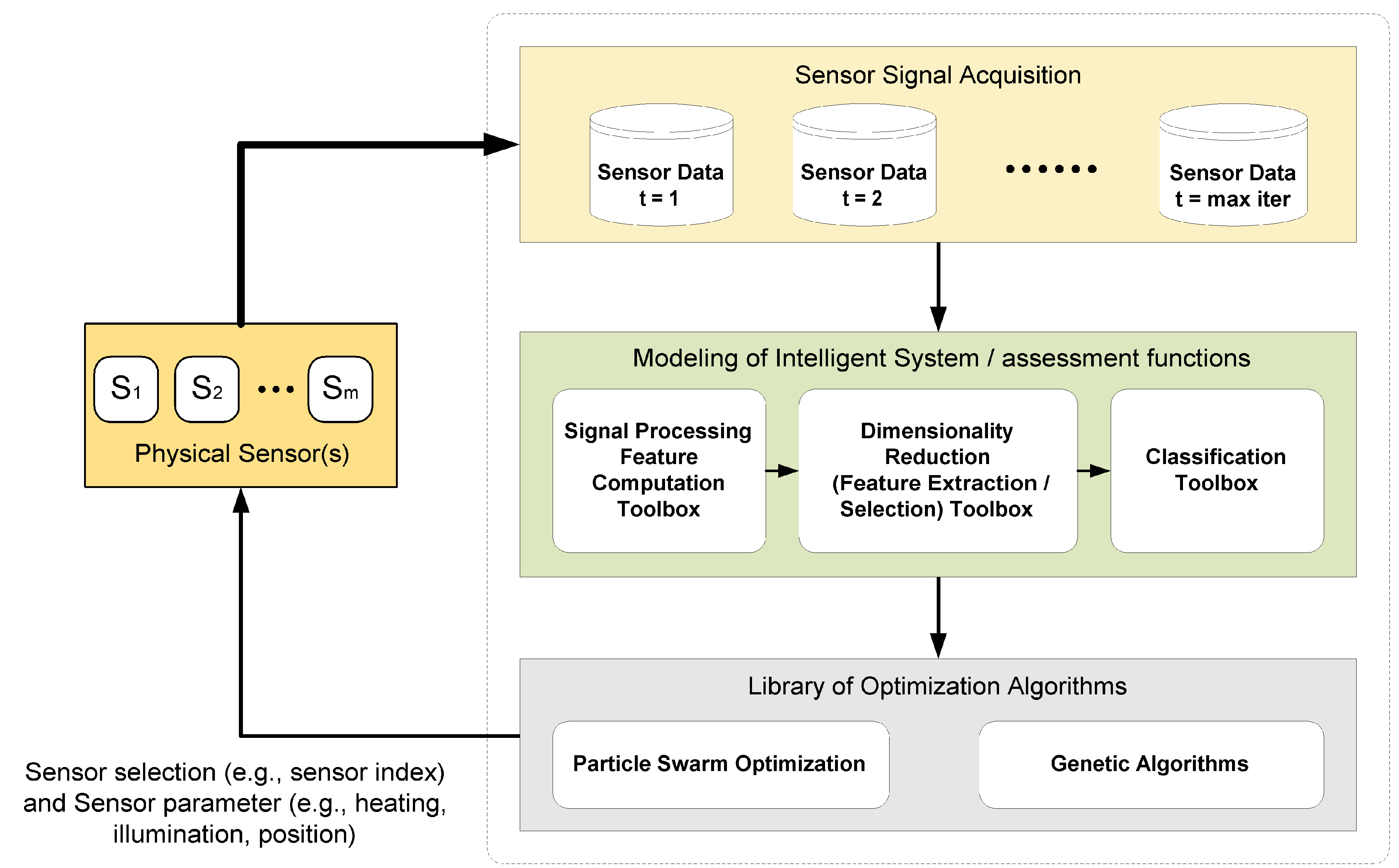
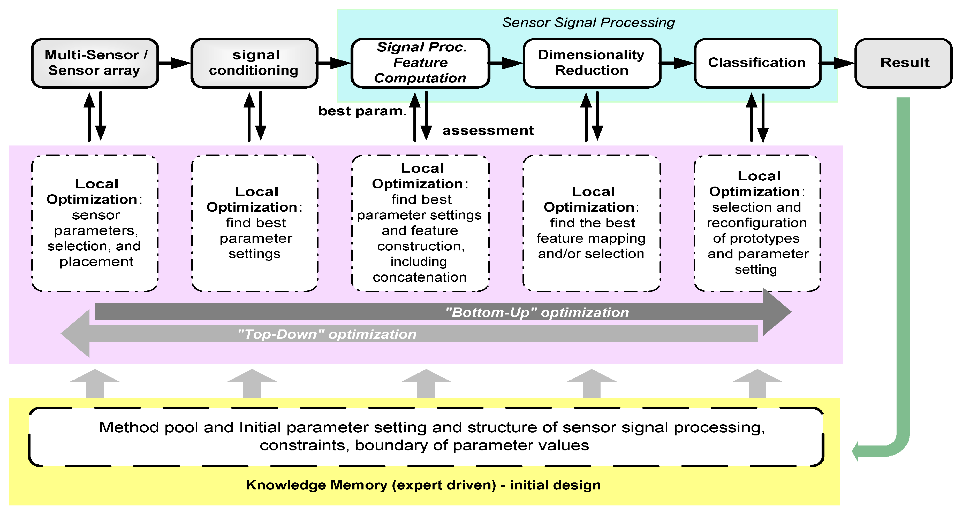
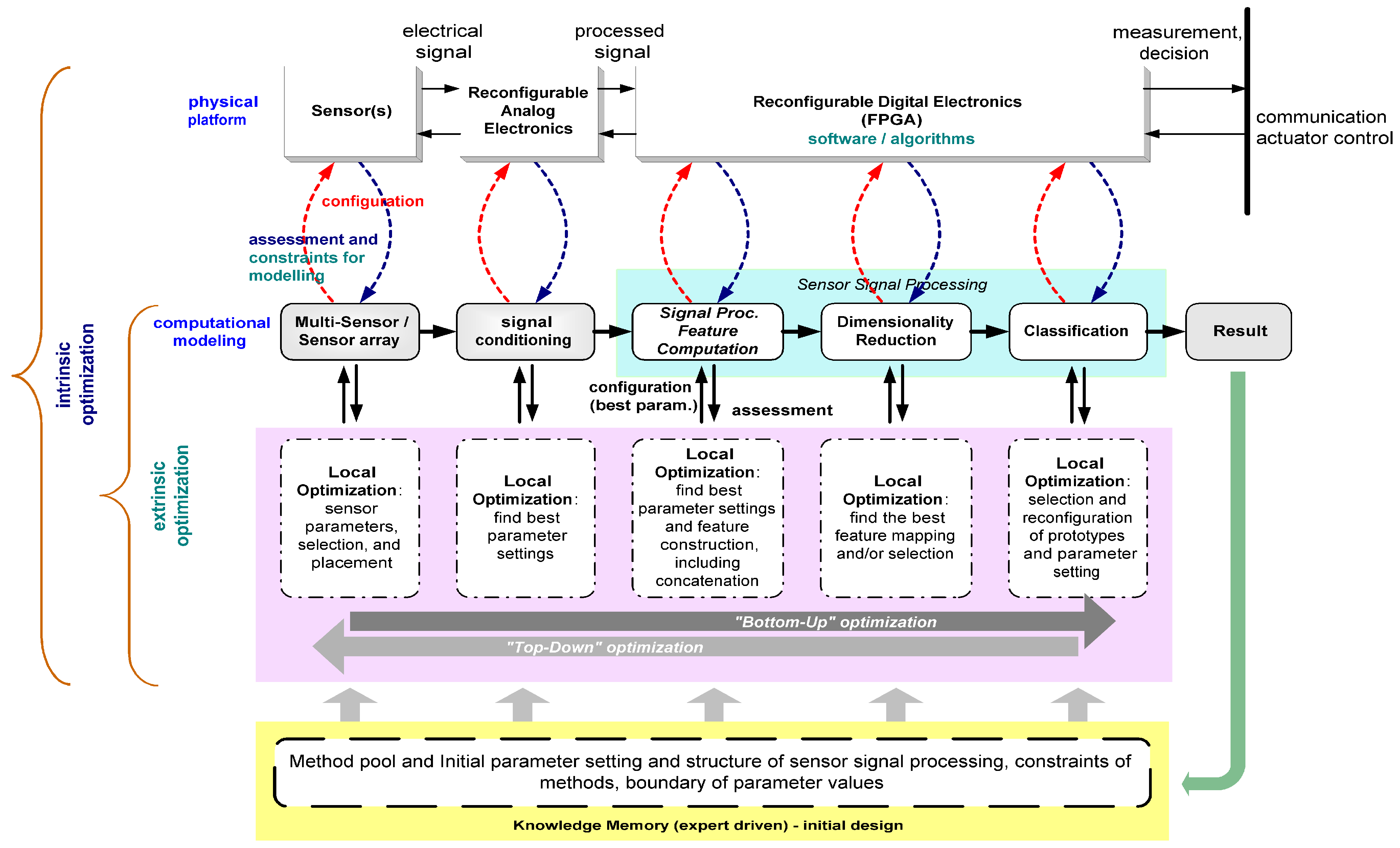
The key optimization tasks in ADIMSS corresponding to Figure 3 are selection and combination; parameter settings and process structure determination [59]; and evolving mapping function. For each optimization task in ADIMSS small adaptations of the optimization algorithms are required. Those modifications mostly occur in the representation of the candidate solutions, the mechanisms of evolving operators (e.g., genetic algorithms) or updating operators (e.g., particle swarm optimization), parameter settings, and the fitness functions. The required modifications have to be specified, when entering a new method to method pool.

Two metaheuristic optimization algorithms, namely, Genetic Algorithms (GA) and Particle Swarm Optimization (PSO), are described briefly in this paper, as well as their modification to cope with our particular design methodology.

3.1. Genetic Algorithm

Genetic algorithms (GA) are search algorithms based on the concept of natural selection and natural genetics [22,23]. GA optimization is a powerful tool with the ability not to get stuck in unfortunate local solutions like gradient descent. This allows one to find feasible and superior solutions in many real applications. Due to this reason, we adopt this optimization concept of GA to solve the problems faced in our design methodology.

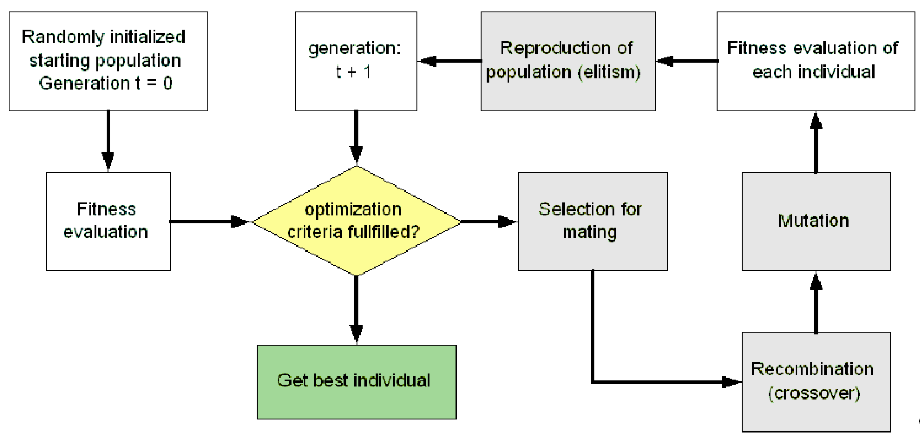
Briefly, the main steps of the GA are initialization (generate an initial population), selection for recombination (e.g., Roulette Wheel Selection or Tournament Selection), recombination (e.g., one point crossover), mutation, selection for reproduction / replacement (e.g., elitism with the best 5–10% of the population), and termination conditions (maximum number of generations exceeded or objective function criteria achieved).

Each candidate solution is referred as an individual or chromosome of a population. An individual encodes a point in the search space of a given problem. The individuals are compared by means of a fitness function. The fitness value is used to guide the recombination and survival of individuals.

A few modifications from the basic concept of GA are needed to cope with our particular system design requirements. The modifications of GA implementation are due to the representation of candidate solutions that are usually composed of heterogeneous structure and different types of values (i.e., binary, integer, and floating-point). Those types of values in the single candidate solution representation usually require properly selected operators (e.g., crossover and mutation) and the combination of those operators. For example, the evolved Gaussian kernels of feature computation reported in [26] applied five different mutation operators to deal with replacement of entire set of solutions, kernel replacement, magnitude adjustment, kernel position adjustment, and kernel width adjustment. Those five mutation operators are controlled by the dynamic weight factor. However, the main steps of GA still remains as shown in Figure 10.

Figure 10. The generalprocess of GA.

Figure 10. The generalprocess of GA.

To find an optimal solution, Genetic Algorithms usually require a large number of individuals in the population (around 50 to 100). Two operators, namely, recombination and mutation, play an important role to increase the population diversity and to ensure the exploration of the search space in finding the best solution.

Recombination (crossover) operators are applied probabilistically according to a crossover rate P_c, which is typically in the range [0.5,1.0]. Usually two parents are selected and then a random variable is drawn from [0,1) and compared to P_c. If the random value is lower than the crossover rate P_c, then two offspring are created via recombination of two parents; otherwise they just copy their parents. Recombination operator can be distinguished into two categories, namely, discrete recombination and arithmetic recombination [48].

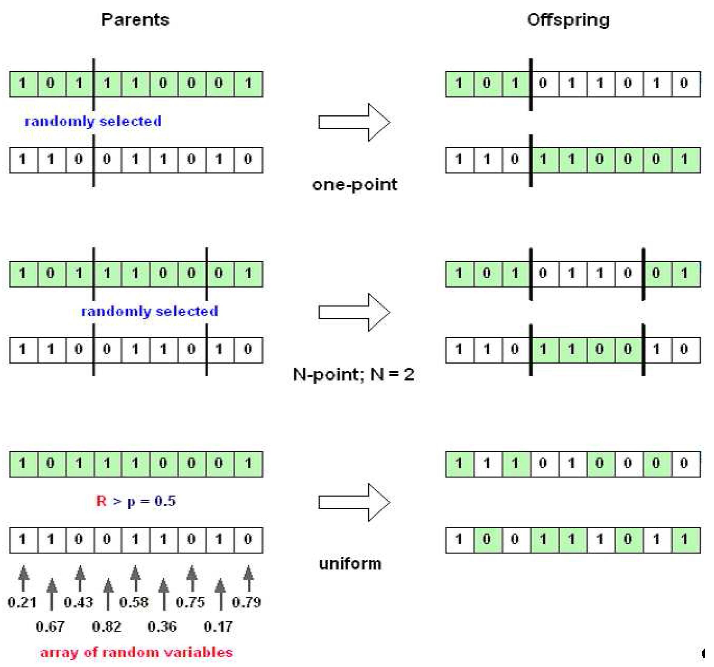
Discrete recombination is the process of exchanging the segments of parents (crossover) to produce offspring, as illustrated in Figure 11. One point crossover works by choosing a random number in the range of the encoding length, then splitting both parents at this point, and creating the two opffspring by exchaning the tails. This operator is mostly used due to the simplicity. One-point crossover can easily be generalised to N-point crossover, where the representation is broken into more than two segments of contiguous genes, and then taking alternative segments from the two parents creates the children. In contrast to those two crossover operators, uniform crossover works by treating each gene independently and making a random choice as to which parent it should be inherited from. This is implemented by generating a string of random variables (equal to the encoding length) from a uniform distribution over [0,1]. In each position, if the value is below a parameter (p = 0.5), then the gene is inherited from the first parent, otherwise from the second. These three crossover operators can be applied for binary, integer, and floating-point representations. However, in the case of real-valued coding (floating-point), these operators have the disadvantage, since these crossover operators only give new combinations of existing values of floating-point. This searching process would rely entirely on the mutation operator. Because of this, another recombination operators for floating-point strings are introduced.

Figure 11. Types of discrete recombination.

Figure 11. Types of discrete recombination.

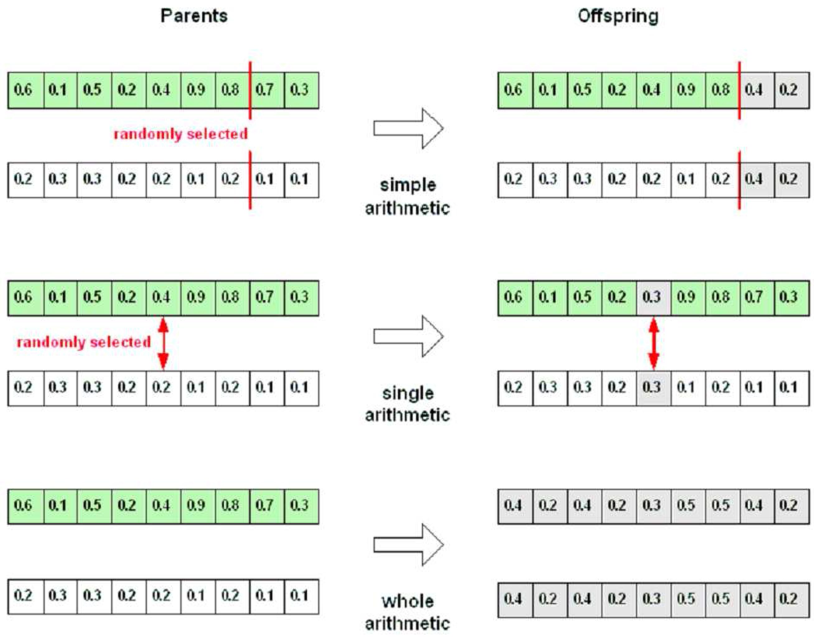
Arithmetic recombination works by creating a new value in the offspring that lies between those of the parents. Those new values can be produced by the following equation:

$$z_i=\alpha x_i+(1-\alpha )y_i$$

(1)

where x_i and y_i are the genes from the first and second parents, respectively, and the α parameter is in the range [0,1]. The types of arithmetic recombination can be recognised through how they select the genes for recombining process. Those are simple arithmetic recombination, single arithmetic recombination, and whole arithmetic recombination. Figure 12 explains the recombination process of all arithmetic recombination operators.

Figure 12. Types of arithmetic recombination; α = 0.5.

Figure 12. Types of arithmetic recombination; α = 0.5.

Mutation is a variation operator that uses only one parent and creates one child. Similar to recombination, the forms of mutation taken depend on the choice of encoding used. The most common mutation operator used for binary encoding considers each gene separately with a small probability P_m (mutation rate) and allows each bit to flip (from 1 to 0 or 0 to 1). It is usually suggested to set a very small value for the mutation rate, from 0.001 to 0.01. For integer encodings, the bit-flipping mutation is extended to random resetting, so that a new value is chosen at random from the set of permissible values in each position with mutation rate P_m. For floating-point representations, a uniform mutation is used, where the values of selected gene x_i in the offspring are drawn uniformly randomly in its domain given by an interval between a lower L_i and upper U_i bound. Table 1 summarizes the most used operators with regard to the representation of individuals.

Table 1. Common recombination and mutation noperators applied for binary, integer, and floating-point representations.

Representation of solutions	Recombination	Mutation
Binary	Discrete	Bit-flipping
Integer	Discrete	Random resetting
Floating-point	Discrete, Arithmetic	Uniform

Table 1. Common recombination and mutation noperators applied for binary, integer, and floating-point representations.

Representation of solutions	Recombination	Mutation
Binary	Discrete	Bit-flipping
Integer	Discrete	Random resetting
Floating-point	Discrete, Arithmetic	Uniform

3.2. Particle Swarm Optimization

Particle swarm optimization (PSO) is a stochastic optimization based on Swarm Intelligence, which also is affiliated to evolutionary computation techniques. Similar to GA, PSO is a population-based search algorithm inspired by the behaviour of biological communities, that exhibit both individual and social behavior, such as fish schooling, bird flocking, swarm of bees, etc. [24].

In PSO, each solution is called a particle. Each particle has a current position in search space, $x_i^t=\langle x_{i,1}^t,x_{i,2}^t,\dots ,x_{i,d}^t\rangle$, a current velocity, $v_i^t$, and a personal best position in search space, $p_i^t$. Particles move through the search space, remembering the best solution encountered. The fitness function is determined by an application-specific objective function. During each iteration, the velocity of each particle is adjusted based on its momentum and influenced by its local best solution $p_i^t$ and the global best solution of the whole swarm $p_g^t$. The particles then move to new positions, and the process is repeated for a prescribed number of iterations. The new velocities and positions in the search space are obtained by the following equations [42]:

$$v_{i,j}^{t+1}=w{v}_{i,j}^t+c_1{r}_1\left(p_{i,j}^t-x_{i,j}^t\right)+c_2{r}_2\left(p_{g,j}^t-x_{i,j}^t\right)$$

(2)

$$x_{i,j}^{t+1}=x_{i,j}^t+v_{i,j}^{t+1}$$

(3)

$$p_i^{t+1}:=\{\begin{array}{ccc}{p}_i^t& if& f(x_i^{t+1})\le f(p_i^t)\\ x_i^{t+1}& if& f(x_i^{t+1})>f(p_i^t)\end{array}$$

(4)

$$p_g^{t+1}:=\{\begin{array}{ccc}{p}_g^t& if& f(p_i^{t+1})\le f(p_g^t)\\ P_i^{t+1}& if& f(p_i^{t+1})>f(p_g^t)\end{array}$$

(5)

Acceleration coefficients c₁ and c₂ are positive constants, referred to as cognitive and social parameters, respectively. They control how far a particle will move in a single iteration. These are both typically set to a value of two [37,43], although assigning different values to c₁ and c₂ sometimes leads to improved performance. r1 and $r_2$ ~ $U\left[0,1\right]$ are values that introduce randomness into the search process, while w is the so called inertia weight, whose goal is to control the impact of the past velocity of a particle over the current one. This value is typically set up to vary linearly from 0.9 to 0.4 during the course of a training run [37,43]. 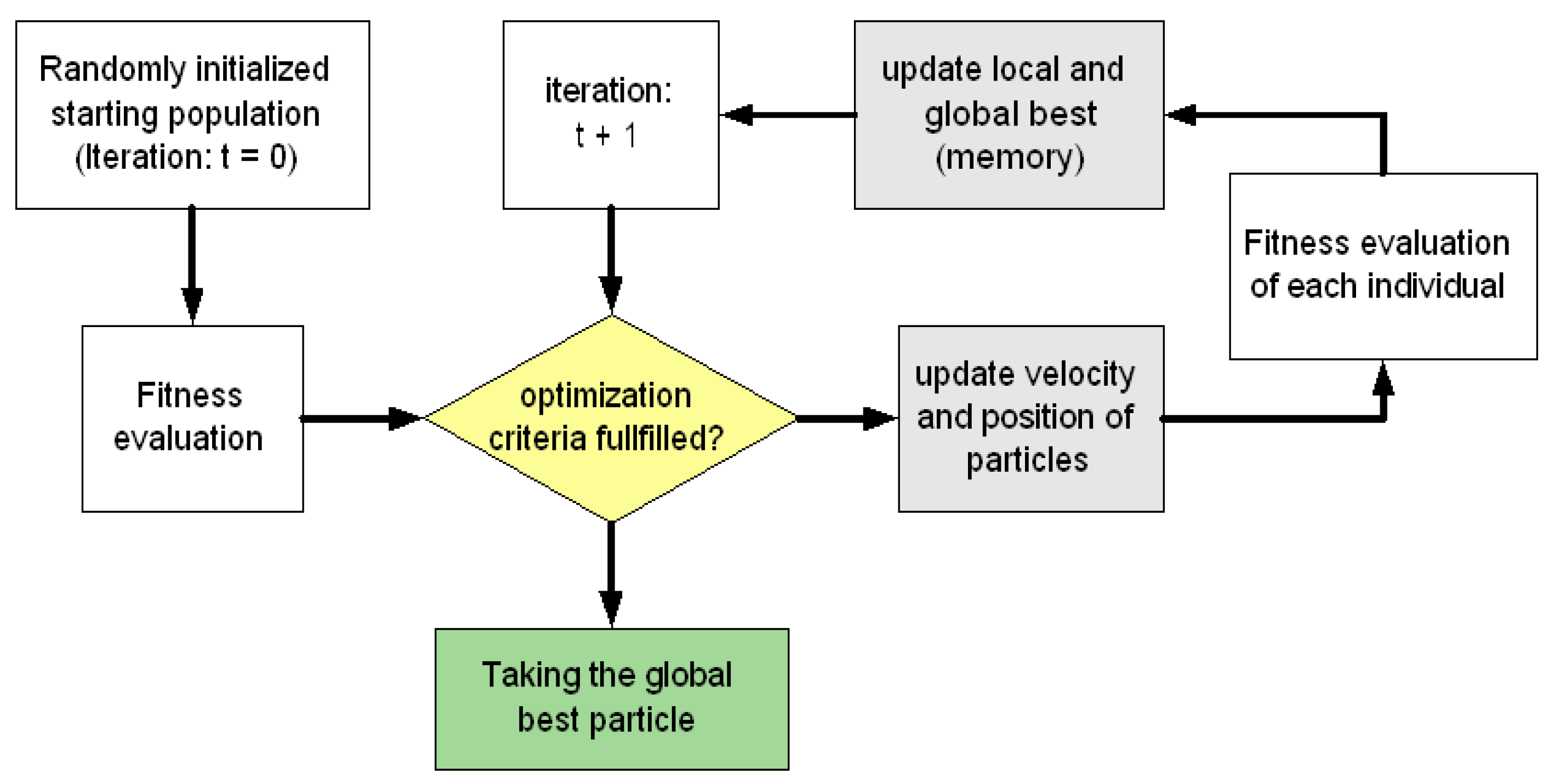Larger values of w at the start of the optimization, allow the exploration of particles into a large area and then, to slightly refine the search space of particles into local optimum by smaller inertia weight coefficients. The general optimization process of PSO is depicted in Figure 13.

Figure 13. The general process of PSO.

Figure 13. The general process of PSO.

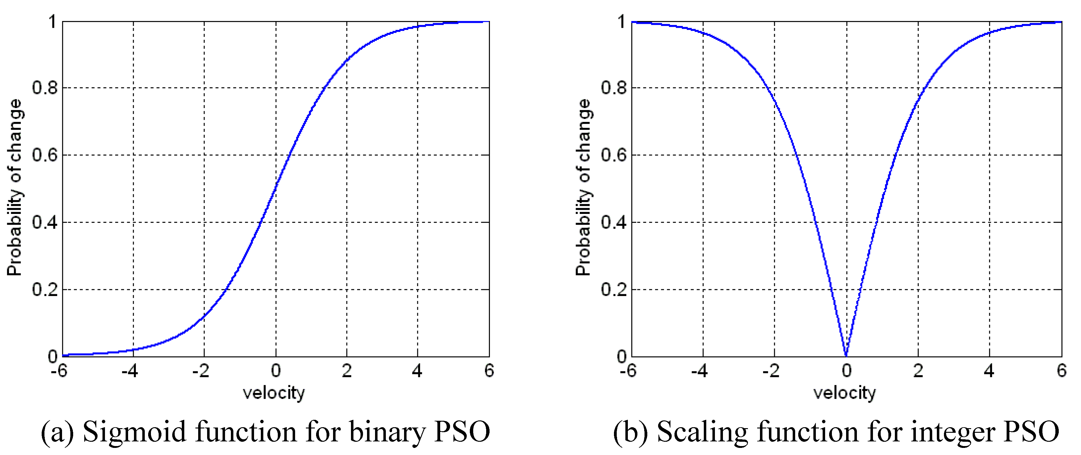
The original PSO explained above is basically designed for real-values (floating–point) problems. Due to the variation in the representation of solution (e.g., binary or discrete and integer), a modification of updating position of particles is required. For a binary representation, the velocity is used to determine a probability threshold. If the velocity is higher, the values of particles are more likely to choose ‘1’, and lower values favor the ‘0’ choice. One of the functions accomplishing this feature is the sigmoid function [25]:

$$s(v_{i,j}^{t+1})=\frac{1}{\left(1+e^{-v_{i,j}^{t+1}}\right)}$$

(6)

Then a new position of particle is computed by the following equation:

$$x_{i,j}^{t+1}:=\{\begin{array}{ccc}1& \text{if}& s(v_{i,j}^{t+1})>\rho \\ 0& \text{if}& s(v_{i,j}^{t+1})\le \rho \end{array}$$

(7)

where ρ is a random numbers from uniform distribution between 0 and 1.

The adaptation approach of PSO for integer representations is based on the binary PSO, where a small modification in the scaling function is required. The outputs of the scaling function are symmetric about 0 and both negative and positive values to lead to high probabilities. The comparison of scaling function used for binary and integer representations is shown in Figure 14. The scaling function [49] is given by:

$$si(v_{i,j}^{t+1})=\frac{2}{\left(1+e^{-\left|v_{i,j}^{t+1}\right|}\right)}-1$$

(8)

The new position of integer PSO is computed by the following equation:

$$\begin{array}{cc}{x}_{i,j}^{t+1}=RandI(),& \begin{array}{cc}\text{if}& rand()<si(v_{i,j}^{t+1})\end{array}\end{array}$$

(9)

where RandI() is a random integer, rand() is a random number from a uniform distribution. However, this approach is suitable for a small range of integer-valued problems and for cardinal attributes (e.g., the compass points). For large ranges of integer-valued problems and ordinal attributes (e.g., 4 is more close to 5 than 30), the adaptation of particle is almost similar to real-value PSO. The difference in the integer PSO from real–valued PSO in equation (3) is that the velocity values are rounded to the nearest integer values. The updated particles are computed as follows:

$$x_{i,j}^{t+1}=x_{i,j}^t+round\left(v_{i,j}^{t+1}\right)$$

(10)

Figure 14. Scaling function of binary PSO based sigmoid function vs. integer PSO.

Figure 14. Scaling function of binary PSO based sigmoid function vs. integer PSO.

3.3. Representation of Individuals

The first stage of developing application-specific algorithms by evolutionary computation (e.g., GA and PSO) is to decide on a representation of a candidate solution to the problem. The representation structure of individuals is identical for both chromosomes in GA and particles in PSO. The representation forms of individuals depend on the type of numbers used to solve a problem. There are three basic types of numbers mostly used in many real problems, namely, binary, integer, and real-valued (floating-point).

Binary representations encode solutions into a string of binary digits (a bit string). In the problems of dimensionality reduction based on automatic feature selection, for instance, the candidate solutions is represented in binary string, where the value of ‘1’ means that elements of the vector are selected and ‘0’ is not selected. Trying to solve a path on a square grid, the compass points {North, East, South, West} could be mapped to a set of values {0,1,2,3} to form a string of integer values (integer representations) for candidate solutions. Real-valued or floating-point representations are the most commonly used in our design type problem. The candidate solution is encoded by a string of real values.

In the proposed ADIMSS tool, the representation of the candidate solutions can be homogeneously one of three types of values or the combination of these three types of values in a vector form. Dealing with mixed type of values, an extra string of information for every segment in the representations of GA or PSO is separately added to select the proper operators. Thus, GA and PSO can properly select the adaptation operators according to this information. This extra information does not evolve during the learning process. The general representation of a candidate solution is described in the following equation:

$$x_i=\left\{G_{i,1},G_{i,2},G_{i,3},\dots ,G_{i,n}\right\}$$

(11)

$$INFO=\left\{Inf{o}_1,Inf{o}_2,Inf{o}_3,\dots ,Inf{o}_n\right\}$$

(12)

$$G_{i,k}=\left\{a_{i,1},a_{i,2},\dots ,a_{i,p}\right\},\begin{array}{cc}& k=1,2,\dots ,n\end{array}$$

(13)

$$Inf{o}_k\in \left\{\text{bin},\text{int},\text{float}\right\}$$

(14)

3.4. Parameter Settings and Knowledge Base

The parameter settings of the optimization algorithms also play an important role to find the best solution. In our automated system design (ADIMSS) tool, the parameters of GA and PSO could be obtained by “trial–and–error” with several fortunate parameters or by automated search using another optimization algorithm. In practice this means that the original optimization problem is now itself run and improved in an additional processing loop, i.e., two nested optimization runs occur. The employment of such a nested optimization approach has to be traded-off with regard to required effort and achievable result quality for each application.

Using the information from the knowledge base or memory block (see Figure 7) to solve similar problems as an initial solution, the effort of nested-loop approach can be reduced due to less search space (intervals). Also, a priori knowledge obtained through experience can be used in the optimization problems with regard to system solutions, parameter settings or intervals, and fusion aspects.

3.5. Assessment Functions and Multi-objective Problem

The evaluation of solutions obtained by the optimization algorithms of ADIMSS is commonly based on classification accuracy. Basically, any classifier can be applied as an assessment function. However, algorithms that possess few parameters are favorable and offer a reliable convergence in training. For instance, the voting k-NN classifier is often applied as an assessment function in automatic feature selection. In the voting k-NN classifier, a test sample is classified in the class represented by a majority of the k number of selected samples. One variant of nearest neighbor methods is the volumetric k-NN, where a test sample is classified in the class represented by the smallest distance among distances between the test sample and the k-th sample in each class. Another variant is the sum-volumetric k--NN [34], which employs the sum of all the k nearest neighbors per class for its decision. The classification performance measure is implemented using the balance accuracy rate, which takes into account the correct classification rate per class. This prevents the searching optimization algorithms from selecting biased models in imbalanced datasets. The assessment function using classification measure is the average of the correct classification as described in the following equation:

$$q_t=\frac{q_{{\omega }_1}+q_{{\omega }_2}+\dots +q_{\omega L}}{L}$$

(15)

where Ω = (ω₁, ω₂, …, ω_L) gives the class affiliation of patterns and q_ω denotes the classification accuracy of a set of patterns with the same class affiliation ω.

The non-parametric overlap measure (NPOM), which is inspired by the nearest neighbor concepts, provides a very fine-grained value range. The NPOM measures the quality of the discriminant data classes in the feature space, where it gives values close to one for non-overlapping class regions and decreases towards zero proportional to increasingly overlapping of class regions. The NPOM is computed by:

$$q_o=\frac{1}{L}{\displaystyle \sum _{c=1}^L\frac{1}{N_c}}{\displaystyle \sum _{i=1}^{N_c}\frac{{\displaystyle {\sum }_{j=1}^k{R}_{i,j}+{\displaystyle {\sum }_{j=1}^k{n}_j}}}{2{\displaystyle {\sum }_{j=1}^k{n}_j}}}$$

(16)

$$n_j=1-\frac{D_{i,j}}{D_{i,k}}$$

(17)

$$R_{i,j}=\{\begin{array}{cc}{n}_i& {\omega }_i={\omega }_j\\ -n_i& {\omega }_i\ne {\omega }_j\end{array}$$

(18)

where n_j computes the weighting factor for the position of the j-th nearest neighbor. D_i,j is the Euclidean distance between the i-th pattern and its j-th nearest neighbor. Ri,j denotes the measure contribution of the i-th pattern with regard to the j-th nearest neighbor. ω_i denotes the class affiliation of the i–th sample, L is the number of classes, and N_c is the number of patterns in the c-th class. Typically, the number of parameter k of this quality measure is set in the range of 5 to 10 [34].

The nonparameteric compactness measure (NPCM) is inspired by linear and non-linear discriminant analysis. The NPCM is applied to measure the quality of the class compactness and separation in the feature space. However, this assessment function still suffers from lack of normalization. The extended version of NPCM is done employing normalized distances (Euclidean distance) [16,34], as shown in the following equation:

$$d{n}_{i,j}=\frac{d_{max}-d_{i,j}}{d_{max}-d_{min}}$$

(19)

where d_i,j is the Euclidean distance between the I–th and the j–th samples. Thus, the normalized NPCM is computed as follows:

$$q_c=w(1-q_{intra})+(1-w)q_{inter}$$

(20)

$$q_{intra}=\frac{1}{L}{\displaystyle \sum _{c=1}^L\frac{2}{N_c(N_c-1)}}{\displaystyle \sum _{i=1}^{N-1}{\displaystyle \sum _{j=i+1}^N\delta ({\omega }_i,{\omega }_j)}}\delta ({\omega }_i,{\omega }_c)d{n}_{i,j}$$

(21)

$$q_{inter}=\frac{1}{NB}{\displaystyle \sum _{i=1}^{N-1}{\displaystyle \sum _{j=i+1}^N\left(1-\delta ({\omega }_i,{\omega }_j)\right)}}{dn}_{i,j}$$

(22)

$$NB={\displaystyle \sum _{i=1}^{N-1}{\displaystyle \sum _{j=i+1}^N\left(1-\delta ({\omega }_i,{\omega }_j)\right)}}$$

(23)

where δ(ω_i, ω_j) is the Kronecker delta, which is δ(ω_i, ω_j) = 1 for ω_i = ω_j (i.e., both patterns have the same class affiliation), and 0 otherwise. N is the number of all patterns. The extended compactness assessment is an aggregation of two assessment functions, i.e., class compactness (q_intra) and separation (q_inter), where it can be considered as a multi-objective function based on weighting method. A user defines the weighting factor, where the default setting of w is 0.5.

Other assessment functions, such as mutual information, entropy [57], and SVM classifier [26], can also be effectively employed in the optimization algorithm to evaluate the candidate solutions. They are the subject of our ongoing studies.

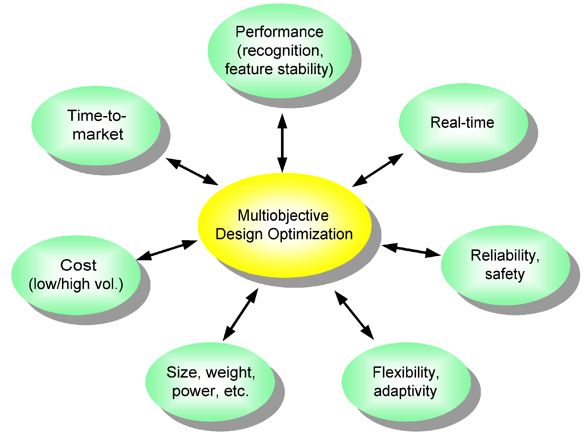
In the proposed ADIMSS, the fitness or assessment function also associates with certain software constraints (e.g., computational complexity, time, stability, etc.) and hardware constraints (e.g., size, speed, memory, timer, counter, power, etc.). Objectives and constraints in design methodology of intelligent multi-sensor systems have been described in Figure 4. Optimizing two or more objective functions, the standard multi-objective optimization approach, in particular, the weighting method is used, since this method is easy to implement. Many objectives are converted to one objective by forming a linear combination of the objectives. Thus, the fitness function is generally described as follows:

$$fitness=\frac{w_1{f}_1+w_2{f}_2+\dots +w_n{f}_n}{{\displaystyle {\sum }_{i=1}^n{w}_i}}$$

(24)

where w_i are called weighting factors, f_i denote assessment values. As GA or PSO parameters, this weigting factors w_i can be determined in two ways, i.e., based on the knowledge of designer (as lucky setting) or based on the systematic search method.

Moreover, to overcome limitations of black-box behavior of the so far described optimization procedures and to add transparency during design, the automated assessment in the ADIMSS tool is complemented by an effective visualization unit, that employs multivariate visualization based on dimensionality reducing mappings, such as the Sammon’s mapping [58]). The visualization unit can be applied by the designer for step-by-step monitoring of the currently achieved pattern discrimination in every part of the whole system during the design process as a visual complement of assessment functions.

4. Sensor Selection and Sensor Parameters

From this section to section seven as shown in Figure 15, we describe the design steps of our design methodology.

Figure 15. Demonstration of the design steps in the ADIMSS automated design methodology.

Figure 15. Demonstration of the design steps in the ADIMSS automated design methodology.

As outlined in the introduction, a large and increasing number of commercial sensors is available on the market. Considering the high number of selectable sensors for an application, finding a good or even optimal solution is not an easy task. Selection of the best sensor is based on the requirements of the measurement system, e.g., accuracy, speed and size, and cost (see Figure 5).

On the other hand, the quality of the solutions obtainable with intelligent multi-sensor systems also depends on sensor parameters and sensor positions. These two conditions can be optimized to increase the results of intelligent sensor systems with regards to classification accuracy. In applications of gas sensor systems, the operating temperature of semiconductor gas sensors is an example of sensor parameter. 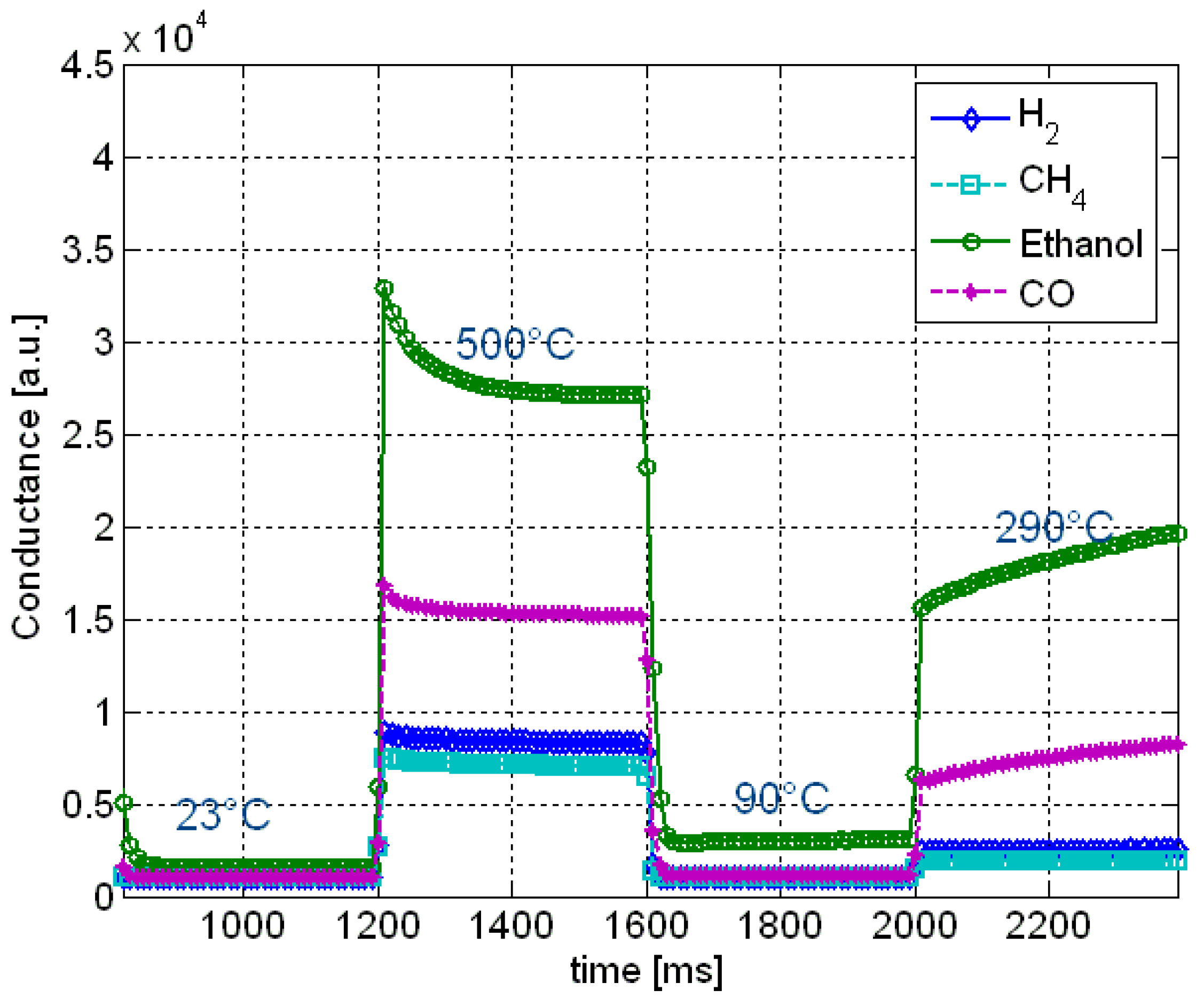The heating element has to be properly controlled to have high sensitivity as well as selectivity [33,34]. Typical sensor response curves are shown in Figure 16. For selected sensors, an optimum heating curve could be evolved.

Figure 16. A snapshot of response curves of a gas sensor is shown for H₂ (7 ppm), CH₄ (1,000 ppm), ethanol (2.4 ppm), and CO (400 ppm) at 70% relative humidity.

Figure 16. A snapshot of response curves of a gas sensor is shown for H₂ (7 ppm), CH₄ (1,000 ppm), ethanol (2.4 ppm), and CO (400 ppm) at 70% relative humidity.

To obtain the best combination of multi-sensor and the optimal sensor parameters, an intrinsic local optimization method is proposed. The local optimization process of intrinsic method is shown in Figure 17, where the sensors are directly connected to the computational model and optimization algorithms. The candidate solution of PSO or GA in this problem represents the indices of selected sensors and their determined sensor parameter settings. The binary representation is used to encode the sensors, where the value of ‘one’ means that sensor is selected and ‘zero’ means the opposite. The multi-sensor can be composed of single sensors and sensor arrays. The sensor parameter can be encoded using either integer representation or floating-point representation, depending on the problems. The representation of a candidate solution is described as follows:

$$x_i=\left\{\langle s_1,s_2,\dots ,s_m\rangle ,\langle h_1,h_2,\dots ,h_m\rangle \right\}$$

(25)

$$INFO=\left\{\langle \text{bin}\rangle ,\langle \text{int}\rangle \right\}$$

(26)

where s_i are a bit value of a sensor, h_i are a parameter value of a sensor, where i = (1, 2, …, m). The fitness of each of candidate solution in the iterations is evaluated by the classification rate. The designer may define a standard model of an intelligent system to evaluate each of the candidate solutions created by optimization algorithms (GA or PSO) with regard to the classification rate. Instead of using such a standard model, other assessment functions based on nearest neighbor methods can also be directly employed to evaluate the candidate solutions. The sensor selection and parameter setting requires intrinsic optimization, which is in this particular case a resource consuming method due to physical stimuli presentations and data acquisition.

Figure 17. An intrinsic method of the local optimization to obtain the optimum multi-sensor and their parameters.

Figure 17. An intrinsic method of the local optimization to obtain the optimum multi-sensor and their parameters.

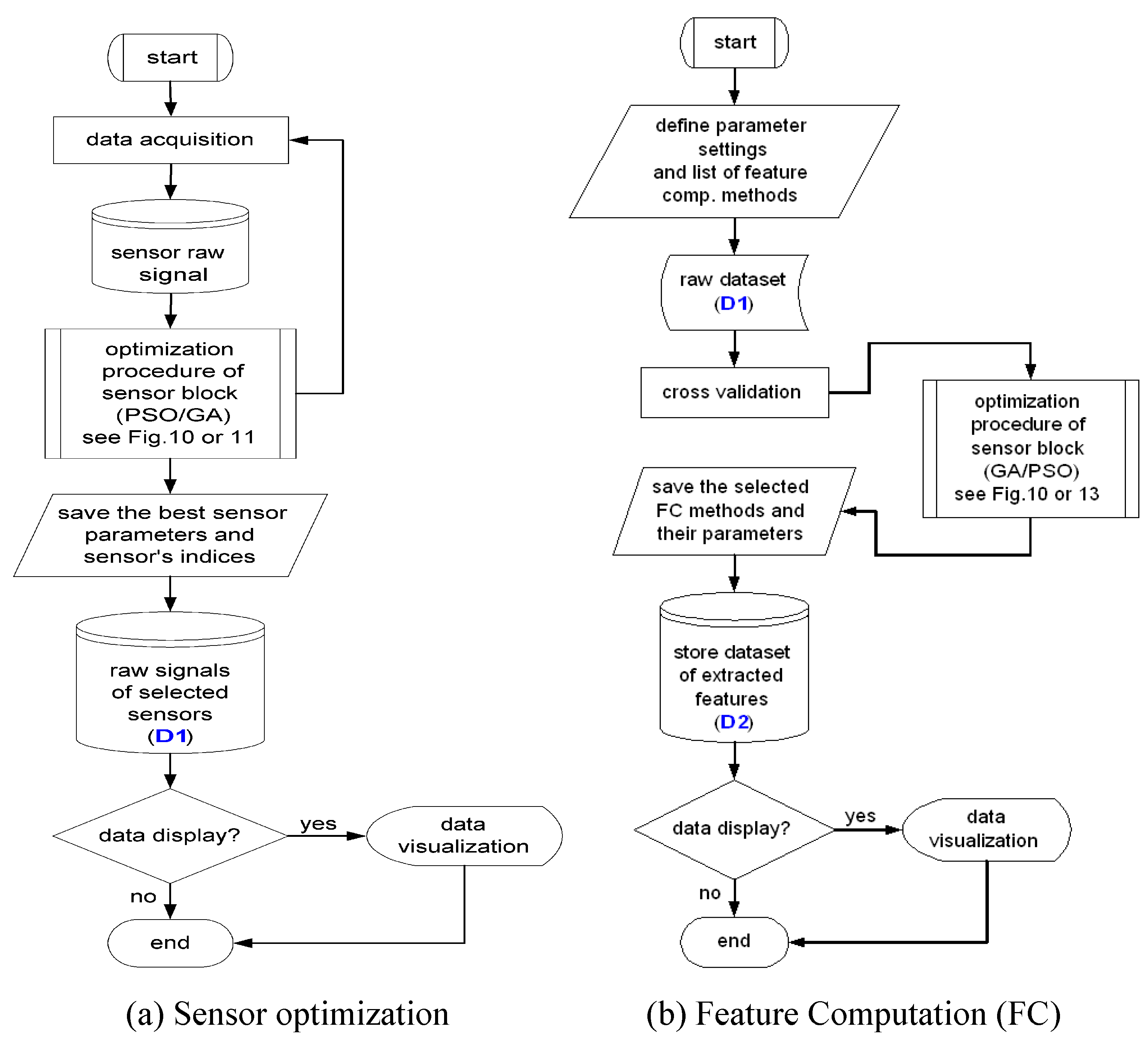
5. Signal Processing and Feature Computation

Sensors often generate data with high dimensionality, therefore extracting the meaningful information of sensor signals requires effective feature computation methods. The next design step in our ADIMSS tool is to obtain the optimal combination of signal processing and feature computation from the method library and to find the best parameter settings. The method library is subject to continuous extension by manually or evolutionarily conceived algorithms.

Signal Pre-processing and Enhancement (SPE) is a first stage of signal processing for noise removal, drift compensation, contrast enhancement and scaling. For example, in the particular case of gas sensor systems, the methods used in the signal prepocessing and enhancement step are differential, relative, fractional [32,35], and derivation [33,36]. In the framework of ADIMSS, the set of operations applied to analyze and extract the features are listed with ID number, which is included in the representation of candidate solutions of PSO or GA. The ID number is evolved in optimization process to indicate the selected method. Table 2 presents a list of signal pre-processing and enhancement, where the method for ID_SPE = 1 is stated as ‘None’, which means that no operation of SPE will be applied.

Table 2. List of signal pre-processing and enhancement methods used for gas sensor systems filled in the design tool of ADIMSS.

IDSPE	Method	Equation
1	None	---
2	Differential	$h(t)=\left(s(t)+{\delta }_a\right)-\left(s(0)+{\delta }_a\right)=\text{}s(t)-s(0)$
3	Relative	$h(t)=\frac{s(t)\left(1+{\delta }_m\right)}{s(0)\left(1+{\delta }_m\right)}=\frac{s(t)}{s(0)}$
4	Fractional	$h(t)=\frac{s(t)-s(0)}{s(0)}$
5	Derivation	$h(t)=s(t)-s(t-1)$

Table 2. List of signal pre-processing and enhancement methods used for gas sensor systems filled in the design tool of ADIMSS.

IDSPE	Method	Equation
1	None	---
2	Differential	$h(t)=\left(s(t)+{\delta }_a\right)-\left(s(0)+{\delta }_a\right)=\text{}s(t)-s(0)$
3	Relative	$h(t)=\frac{s(t)\left(1+{\delta }_m\right)}{s(0)\left(1+{\delta }_m\right)}=\frac{s(t)}{s(0)}$
4	Fractional	$h(t)=\frac{s(t)-s(0)}{s(0)}$
5	Derivation	$h(t)=s(t)-s(t-1)$

Common types of features mostly extracted from raw sensor signals are the geometric attributes of signal curve (e.g., steady state, transient, duration, slope, zero-crossings), statistical feature (mean, standard deviation, minimum, maximum, etc.), histogram, spectral peaks (Fourier Transform), Wavelet Transform, Wigner–Ville Transform, auditory feature for sound and speech signals, etc. Table 3 summarizes a small list of feature computation methods. Here, two operators of heuristic feature computation (i.e., Multi–level thresholding and Gaussian Kernels) applied in gas sensor systems are picked up as examples to demonstrate the autoconfiguration of feature computation in the proposed ADIMSS tool.

Table 3. List of operators for extracting of features used in sensor signal processing (e.g., gas detection).

IDFC	Method	Parameter
1	Steady-state	none
2	Transient integral	none
3	Histogram	range of bins, down_bnd, up_bnd
4	MLT	thresholds (TL); L = 1, 2, …, n
5	GWF	μk, σk, Mk; k = 1, 2, …, n
6	Spectral peaks (FFT)	None

Table 3. List of operators for extracting of features used in sensor signal processing (e.g., gas detection).

IDFC	Method	Parameter
1	Steady-state	none
2	Transient integral	none
3	Histogram	range of bins, down_bnd, up_bnd
4	MLT	thresholds (TL); L = 1, 2, …, n
5	GWF	μk, σk, Mk; k = 1, 2, …, n
6	Spectral peaks (FFT)	None

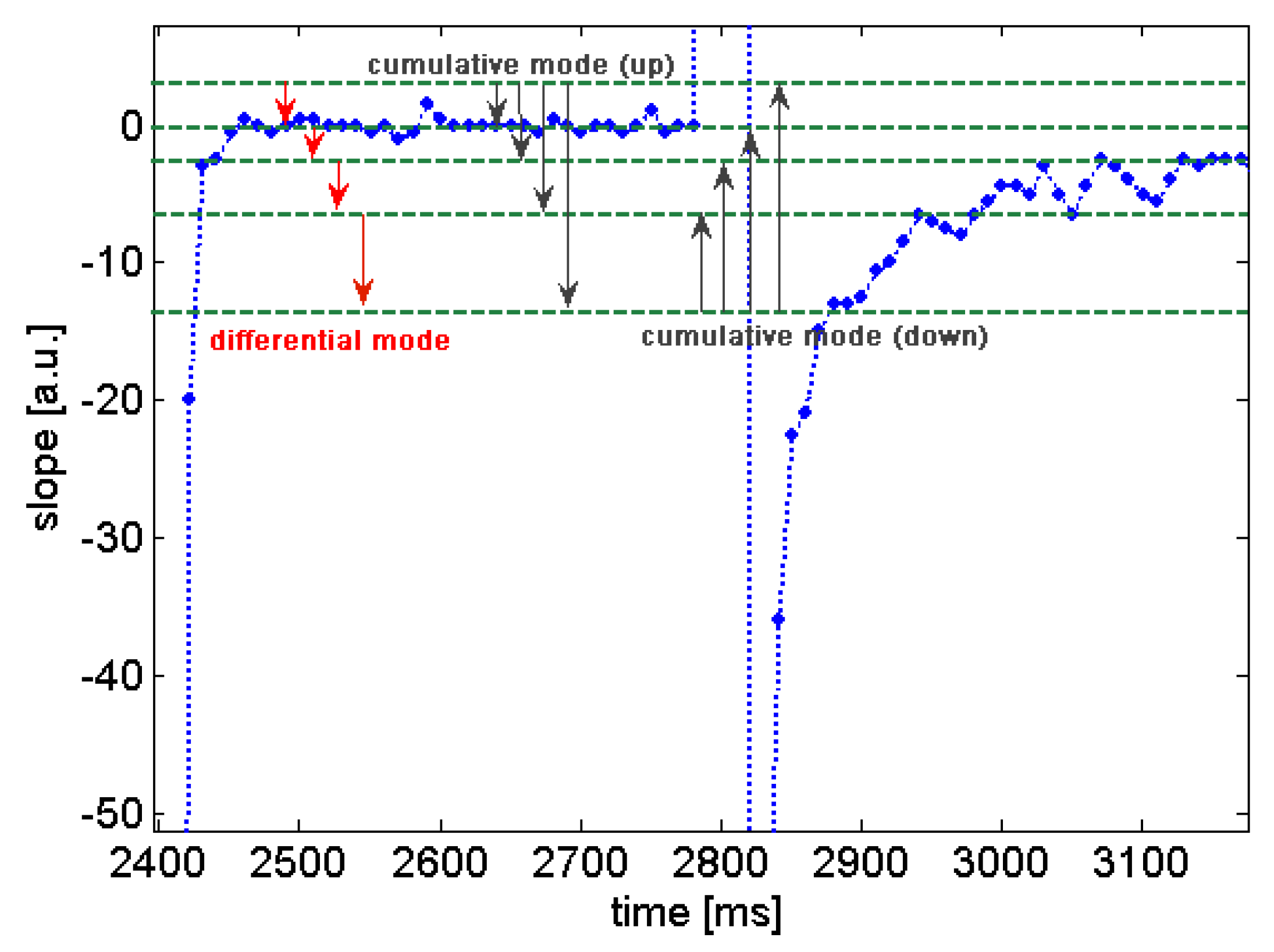
Multi-level thresholding (MLT) operators are a heuristic feature computation method that extracts the features by counting samples of signal responses lying in the range between two thresholds. MLT is derived from histogram and amplitude distribution computation by non-equal range of bins [15]. Figure 18 illustrates differential and cumulative (up and down) modes of MLT computation. The MLT is optimized by moving of the levels up and down until the optimal solution with regard to the classification rates and other assessment criteria achieved. The number of features extracted by MLT depends on the number of thresholdings minus one. In the optimization process, the numbers of thresholds are swept from 3 to 10 (the maximum number of thresholds can be defined by designer) and in each sweep the positions of the current set of thresholds are optimized based on the assessment function (e.g., the quality overlap measure). In the end of the optimization process, the optimum solutions are selected by the aggregating function of the assessment function and the number of thresholds used.

Figure 18. Multi-level thresholding used for extracting features of slope curves of gas sensors. MLT is modified from histogram and amplitude distribution computation by non-equal range of bins. Three methods of MLT are differential, cumulative (up) and cumulative (down) modes.

Figure 18. Multi-level thresholding used for extracting features of slope curves of gas sensors. MLT is modified from histogram and amplitude distribution computation by non-equal range of bins. Three methods of MLT are differential, cumulative (up) and cumulative (down) modes.

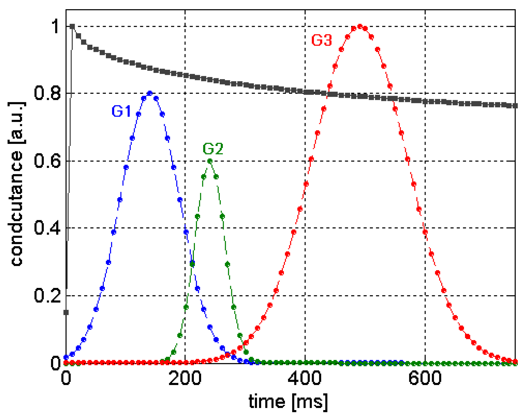
The Gaussian window function (GWF) method computes features from sensor signals based on the product of two vectors, i.e., a sensor signal and Gaussian function. The GWF method consists of many kernels, which are Gaussian exponential functions with different means μ_i, standard deviations σ_i, and magnitudes M_i, where i = 1, 2, …, k. Those three parameters represent the position, width, and the height of kernels (see Figure 19). The extracted features of GWF and Gaussian kernel function [26,37] are defined as follows:

$$f_i={\displaystyle \sum _{s=1}^N{x}_s}G(s,M_i,{\mu }_i,{\sigma }_i)$$

(27)

$$G(s,M_i,{\mu }_i,{\sigma }_i)=M_i{e}^{-\frac{1}{2}{\left(\frac{s-{\mu }_i}{{\sigma }_i}\right)}^2}$$

(28)

where x_s is a measurement value of sensor signal at sampled time index s = 1, 2, …, N. The magnitudes of kernels is in the range from ‘0’ to ‘1’. The optimization strategy of GWF is different from MLT optimization, where the number of kernels evolves according to values of M_i. If the values of M_i are zero, then those kernels can be discarded. The maximum number of kernels is defined by the designer.

Figure 19. Evolving Gaussian kernels used for extracting features of gas sensor responses.

Figure 19. Evolving Gaussian kernels used for extracting features of gas sensor responses.

Table 4 gives the details of the parameter settings of PSO and GA related to the methods of feature computation in the experiments of the benchmark gas dataset [15]. Those parameter settings of PSO and GA are defined by the designer manually (as lucky parameters). However, in the automated system design, the parameters of optimisation algorithms can be defined by the nested optimization approach. Both PSO and GA employed for finding the proper configuration of extracting features using the MLT methods have proved to overcome the suboptimum solution given by expert designer as shown in Table 5.

Table 4. Parameter settings of GA and PSO.

MLT-DM-GA / MLT-CM-GA	MLT-DM-PSO / MLT-CM-PSO	GWF-GA
Population = 20 Selection = Roulette Wheel Recombination = discrete; Pc = 0.8 Mutation = uniform; Pm = 0.01 Elitism = 10% Maximum generation = 100 Assessment fcn = NPOM (k = 5)	Population = 20 wstart = 0.9; wend = 0.4 c1 = 2; c2 = 2 Update fcn = floating-point Maximum generation = 100 Assessment fcn = NPOM (k = 5)	Population = 20 Selection = Tournament Recombination = discrete; Pc = 0.85 Mutation = uniform; Pm = 0.1 Elitism = 10% Maximum generation = 100 Assessment fcn = k-NN (k = 5)

Table 4. Parameter settings of GA and PSO.

MLT-DM-GA / MLT-CM-GA	MLT-DM-PSO / MLT-CM-PSO	GWF-GA
Population = 20 Selection = Roulette Wheel Recombination = discrete; Pc = 0.8 Mutation = uniform; Pm = 0.01 Elitism = 10% Maximum generation = 100 Assessment fcn = NPOM (k = 5)	Population = 20 wstart = 0.9; wend = 0.4 c1 = 2; c2 = 2 Update fcn = floating-point Maximum generation = 100 Assessment fcn = NPOM (k = 5)	Population = 20 Selection = Tournament Recombination = discrete; Pc = 0.85 Mutation = uniform; Pm = 0.1 Elitism = 10% Maximum generation = 100 Assessment fcn = k-NN (k = 5)

Table 5. Results of MLT-DM and MLT-CM configured by human expert (Manual), GA and PSO (Automated) and result of GWF configured by GA (Automated).

Method	qo	k-NN (%) with k = 5	Thresholds or Kernels
MLT-DM	0.982	99.17	13
MLT-DM – GA	0.995	99.67	9
MLT-DM – PSO	1.00	100	9
MLT-CM	0.956	97.17	5
MLT-CM – GA	0.988	99.50	5
MLT-CM – PSO	0.995	99.92	5
GWF – GA	0.991	98.46	3

Table 5. Results of MLT-DM and MLT-CM configured by human expert (Manual), GA and PSO (Automated) and result of GWF configured by GA (Automated).

Method	qo	k-NN (%) with k = 5	Thresholds or Kernels
MLT-DM	0.982	99.17	13
MLT-DM – GA	0.995	99.67	9
MLT-DM – PSO	1.00	100	9
MLT-CM	0.956	97.17	5
MLT-CM – GA	0.988	99.50	5
MLT-CM – PSO	0.995	99.92	5
GWF – GA	0.991	98.46	3

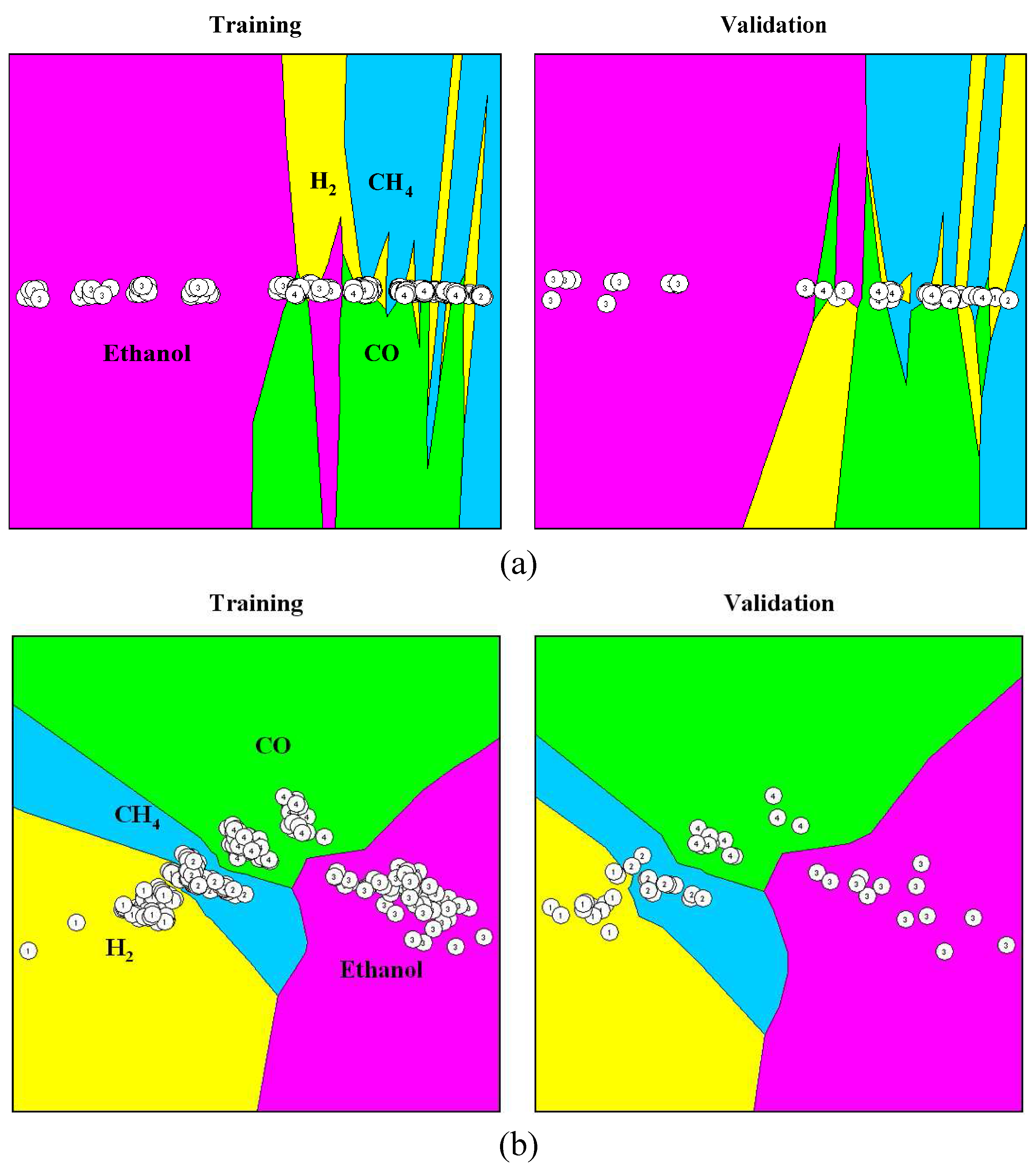
As mentioned in Subsection 3.5, multivariate visualization can be employed effectively to provide insight into the achieved solutions to the designer. Figure 20 shows an example of multivariate data visualizations of four gases extracted by evolved Gaussian kernels, where the discrimination of patterns with regard to their class affiliation is clearly depicted.

Figure 20. Visual inspection of four gases data: (a) raw sensor signals and (b) extracted by evolved Gaussian kernels.

Figure 20. Visual inspection of four gases data: (a) raw sensor signals and (b) extracted by evolved Gaussian kernels.

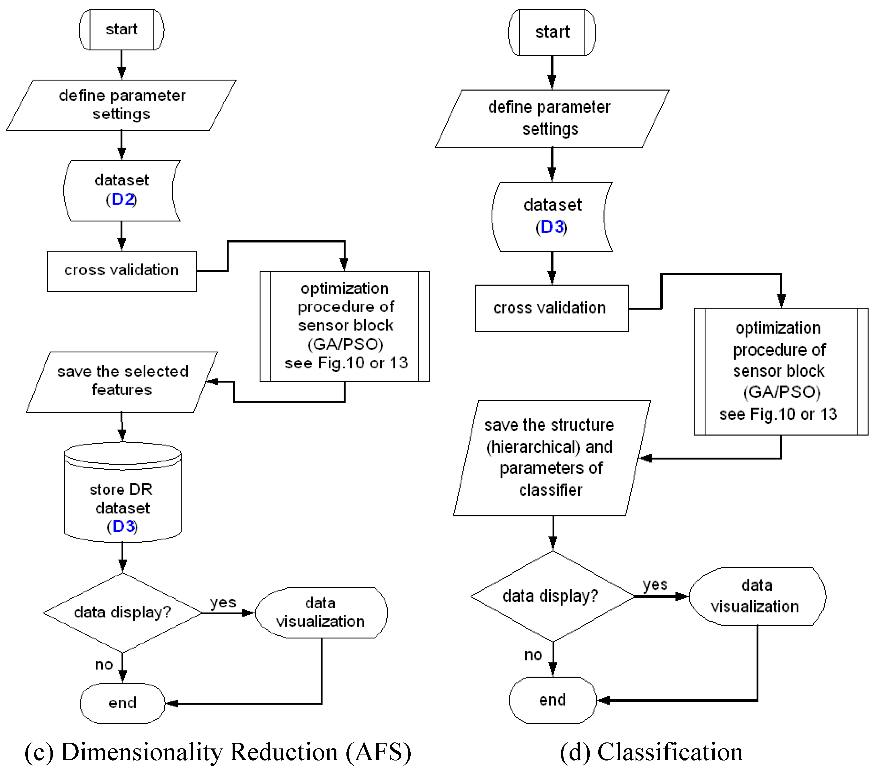
6. Dimensionality Reduction

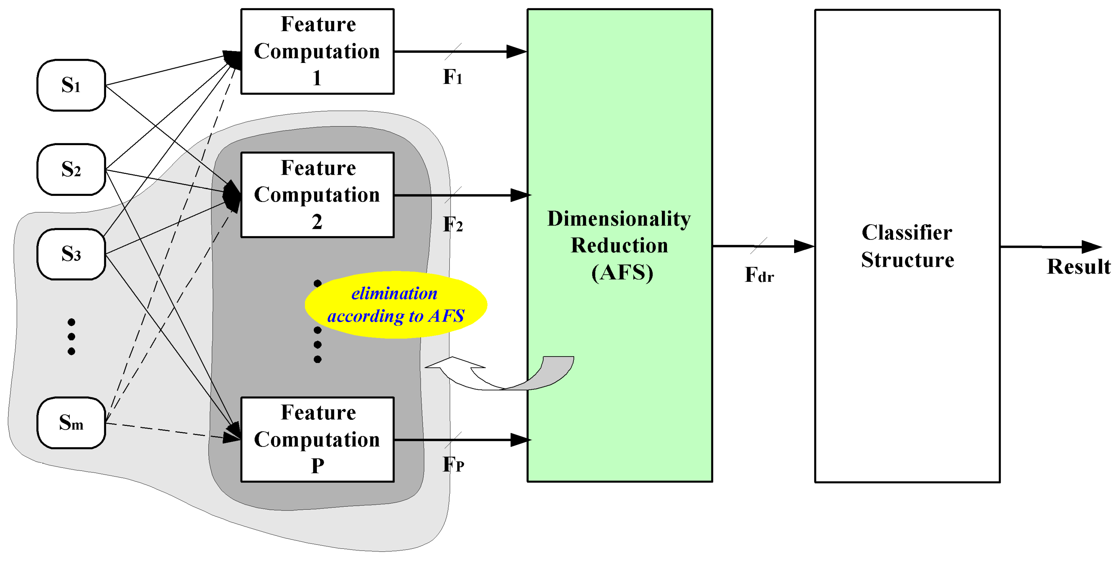
In this section, we show the dimensionality reduction aspects related to our automated system design methodology. There are many available methods used for dimensionality reduction, i.e., principle component analysis (PCA), linear discriminant analysis (LDA), projection pursuit, multi–dimensional scaling (MDS), etc. [18,58]. A special case of dimensionality reduction described here is feature selection. Feature selection is a method to find minimum feature subset giving optimum discrimination between two or more defined groups of objects. This method is an iterative algorithm, also called Automatic Feature Selection (AFS). This approach is applied for optimized sensor system design by reducing or discarding the irrelevant or redundant features or groups of features, which are extracted by feature computation methods at previous stage. Moreover, the sensorial effort will be saved due to efficient selection. Figure 21 describes the elimination process of unnecessary features or groups of features, as well as sensors.

Basically, the AFS can be divided into two groups, i.e., (1) wrapper method that is performed dependently of the learning algorithm or classifier (e.g., RBF, SVM, etc.); and (2) filter approach that utilizes various statistical techniques underlying training data and operates independently of the classifier [51]. In general, the wrapper method provides selected features that lead to more accurate classifications than that of the filter method. However, the filter method executes many times faster than the wrapper method.

Figure 21. Process of intelligent multi-sensor system design focused on the structure optimization by elimination of redundant feature computation and sensors.

Figure 21. Process of intelligent multi-sensor system design focused on the structure optimization by elimination of redundant feature computation and sensors.

6.1. AFS with Acquisition Cost

In designing an intelligent sensor system, the objective function of the AFS in the optimization tool (ADIMSS) is often associated with certain cost. The aim of the AFS with acquisiton Cost (AFSC) is to discard the unnecessary and expensive features. The accumulative expression of the objective function is:

$$fitness=w_{1}q+w_2\left(1-\frac{C_s}{C_t}\right)+w_3\left(1-\frac{f_s}{f_t}\right)$$

(29)

where q can be the quality of overlap measurement given in subsection 3.5 and/or the classification rate depending on the user selection, wi are weighting factor with ${\displaystyle {\sum }_{i=1}^3{w}_i}=1$. C_s denotes the sum of costs from selected features, C_t denotes the sum of total cost from all features, f_s is the number of selected features, and f_t is the number of whole features. Table 6 shows one example of defining the cost value by designer for each mathematical operation used to extract features in feature computation methods.

Table 6. The cost values for basic operations mostly used to evaluate the computational effort of methods of feature computation.

No.	Operation	Cost
1	Addition (+)	1
2	Substraction (-)	1
3	Multiplication (*)	4
4	Substraction (/)	4
5	Comparison (>,≥, ≤,<, =, ≠)	2
6	Root square	6
7	Exponential (ex)	8
8	logarithm	8

Table 6. The cost values for basic operations mostly used to evaluate the computational effort of methods of feature computation.

No.	Operation	Cost
1	Addition (+)	1
2	Substraction (-)	1
3	Multiplication (*)	4
4	Substraction (/)	4
5	Comparison (>,≥, ≤,<, =, ≠)	2
6	Root square	6
7	Exponential (ex)	8
8	logarithm	8

Table 7 gives the details of the parameter settings of PSO and GA with regard to the automated design activities based on automatic feature selection with acquisition cost and the cost assignment of eye image dataset. Again, these parameter settings of PSO and GA are heuristically set based on the knowledge base. The cost assignment for the three feature computation operators is determined with regard to the number of multiplication and addition operations. In these experiments, the assuming multiplication has the cost of 10 additions. Therefore, the cost of each feature for Gabor filter, ELAC, and LOC is determined as shown in Table 7. From the experimental results shown in Table 8, the AFSC employing PSO or GA can select low cost and less number of features (i.e., six of 58 features).

Table 7. Parameter settings of GA and PSO, as well as the acquisition cost

AFS - GA	AFS - PSO	Eye image data
Population = 20 Selection = Roulette Wheel Recombination = discrete; Pc = 0.8 Mutation = uniform; Pm = 0.01 Elitism = 10% Maximum generation = 100 Assessment fcn = NPOM (k = 5)	Population = 20 wstart = 0.9; wend = 0.4 c1 = 2; c2 = 2 Update fcn = binary Maximum generation = 100 Assessment fcn = NPOM (k = 5)	Gabor filter = 12 features ELAC = 13 features LOC = 33 features Cost: Gabor filter = 6358 per feature ELAC = 3179 per feature LOC = 1445 per feature

Table 7. Parameter settings of GA and PSO, as well as the acquisition cost

AFS - GA	AFS - PSO	Eye image data
Population = 20 Selection = Roulette Wheel Recombination = discrete; Pc = 0.8 Mutation = uniform; Pm = 0.01 Elitism = 10% Maximum generation = 100 Assessment fcn = NPOM (k = 5)	Population = 20 wstart = 0.9; wend = 0.4 c1 = 2; c2 = 2 Update fcn = binary Maximum generation = 100 Assessment fcn = NPOM (k = 5)	Gabor filter = 12 features ELAC = 13 features LOC = 33 features Cost: Gabor filter = 6358 per feature ELAC = 3179 per feature LOC = 1445 per feature

Table 8. The AFS and AFSC results for eye-image data [19].

Method	Cost	Feature	9-NN (%)	RNN (%)	NNs (%)
without AFS	165308	58	96.72	80.33	97.87
AFS-GA	53176	16	98.36	95.08	96..81
AFSC-GA	13872	6	96.72	95.08	96.81
AFS-PSO	45951	18	100	95.08	98.94
AFSC-PSO	10404	6	96.72	98.36	98.94

Table 8. The AFS and AFSC results for eye-image data [19].

Method	Cost	Feature	9-NN (%)	RNN (%)	NNs (%)
without AFS	165308	58	96.72	80.33	97.87
AFS-GA	53176	16	98.36	95.08	96..81
AFSC-GA	13872	6	96.72	95.08	96.81
AFS-PSO	45951	18	100	95.08	98.94
AFSC-PSO	10404	6	96.72	98.36	98.94

6.2. Effective Unbiased Automatic Feature Selection

AFS techniques try to find the optimum feature set based on the corresponding training set. Interchange of the training and test sets or even smaller changes in the data can dramatically effect the selection. Thus, the issue of selection stability arises, in particular for small sample cases, which heretofore has been largely unanswered. For this reason, in this approach the AFS is augmented by cross-validation (CV), which is a well known method for classifier error estimation. The aim of applying CV is to perturb the training set to obtain selection statistics and information on most frequently used (stable) features [16,50]. For instance, the leave-one-out (LOO) method is implanted within the AFS procedure, where the LOOFS will take place based on (N – 1) samples from the training set for N runs. First and second order statistics can be generated from these N selection results by incrementing the bins ρ_i for the selected features, or ρ_ij for selected feature pairs, respectively. The first and second order statistics of features is normalized by N. Three methods have been introduced in [50], namely, Highest Average Frequency (HAF), Elimination Low Rank Feature (ELRF), and Neighborhood-Linkage Feature (NLF). The first two approaches (HAF and ELRF) determine the unbiased features based on first order statistics, and the NLF is based on first and second order statistics.

The HAF approach is to seek the optimal feature subset among N solutions produced by LOOFS, where each solution of active features is multiplied with their probability of the first order statistic and normalized by the number of active features. A solution is selected from the collection of solutions found by LOOFS in N runs, if its average frequency is the highest. Let F_n = (f_n,1, f_n,2, …, f_n,M) be a solution of consisting M features and F_n be a binary-vector, where n = {1, 2,…, N}. The average frequency is defined as:

$$P_n=\frac{{\displaystyle {\sum }_{i=1}^M{f}_{n,i}{\rho }_i}}{A}$$

(30)

where A denotes the number of active features.

The ELRF approach is to seek the unbiased feature subset, where the probability of selected features is above a computed threshold. The ELRF ranks the features based on the frequency of first order histogram from highest to lowest frequency and recomputes the first order histogram as follows:

$$R_i=\frac{{\displaystyle {\sum }_{j=1}^i{{\rho }^{\prime }}_j}}{i}$$

(31)

where ${{\rho }^{\prime }}_j$ is the probability value of the j-th feature after ranking arrangement and i is the rank index. The threshold is computed as follows:

$$T=\frac{{\displaystyle {\sum }_{i=1}^M{R}_i}}{M}$$

(32)

where M is the number of features.

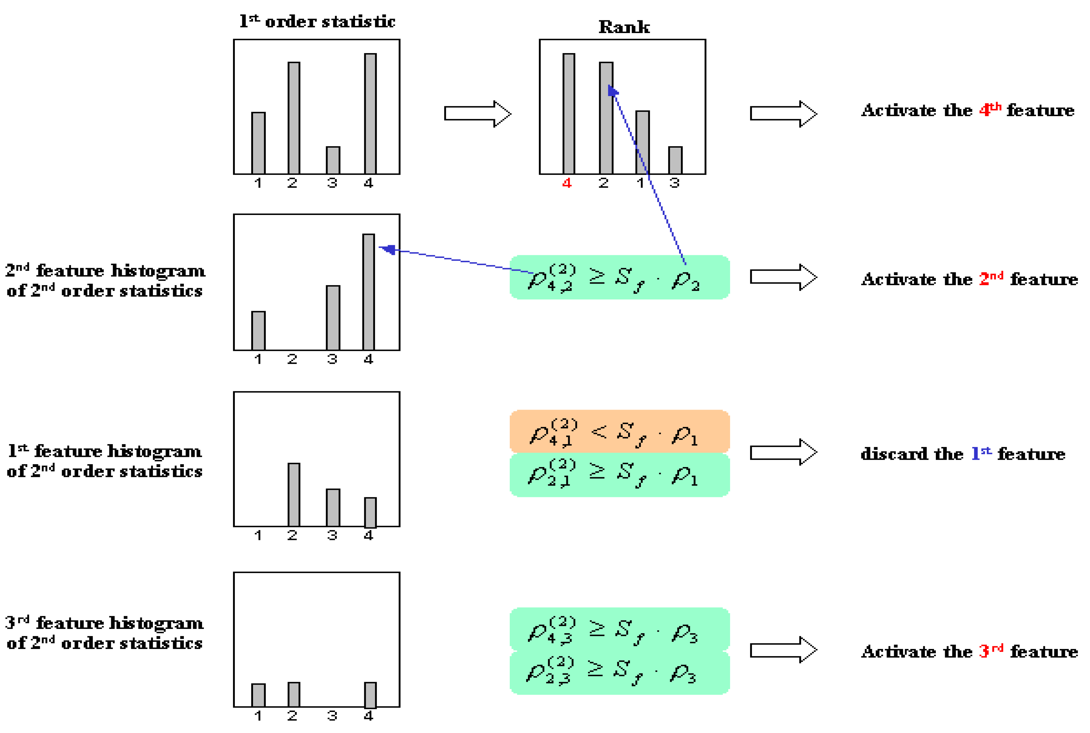
In the NLF approach, first order statistics is used as a reference to determine the rank of the features. In this approach the highest rank feature will be selected or activated automatically. The rest of lower rank features will be evaluated by referring to the active higher rank features. If the evaluation of one feature fails to even a single of its active higher rank features, the feature will be discarded, otherwise it will be selected and participated into evaluating process for the next lower rank features. This selection process is described in more detail in Figure 22.

Figure 22. The evaluating procedure of NFL approach.

Figure 22. The evaluating procedure of NFL approach.

The evaluation process is determined by the following equation:

$${\rho }_{i,j}^{(2)}\ge S_f{\rho }_j$$

(33)

where ${\rho }_{i,j}^{(2)}$ are the 2^nd order frequencies of selected the j-th feature when the i-th feature is selected, and S_f denotes the selection stability measurement [16]. Here, the selection stability function is modified to give proportional assessment value for all possible cases. The selection stability measurement is defined by following equation:

$$S_f=\left({\rho }_{\max }-{\rho }_{\min }\right)\frac{U+f_z}{B+f_h+f_z}$$

(34)

where the value of S_f is in the range between 0 (the worst case situations) and 1 (the best stability). U denotes the accumulation of all frequencies, which are larger than half of the maximum frequency value. B denotes the accumulation of all frequencies, which are lower than half of the maximum frequency value. f_z is the number of features which their frequency values are equal zero. f_h is the number of features which their frequency values are larger than half of the maximum frequency value. This selection stability criterion indicates the aptness of feature selection for the regarded task and data.  In these experiments, we applied benchmark datasets from repository and real application, i.e., wine, rock, and eye-tracking image to give a perspective of using these approaches in the sensor system design. Details of the benchmark datasets are given in Table 9.

Table 9. Summary of the benchmark datasets [16].

Dataset	Feature	Class	Samples
Wine	13	3	59 / 71 / 48
Rock	18	3	31 / 51 / 28
Eye image	58	2	105 / 28

Table 9. Summary of the benchmark datasets [16].

Dataset	Feature	Class	Samples
Wine	13	3	59 / 71 / 48
Rock	18	3	31 / 51 / 28
Eye image	58	2	105 / 28

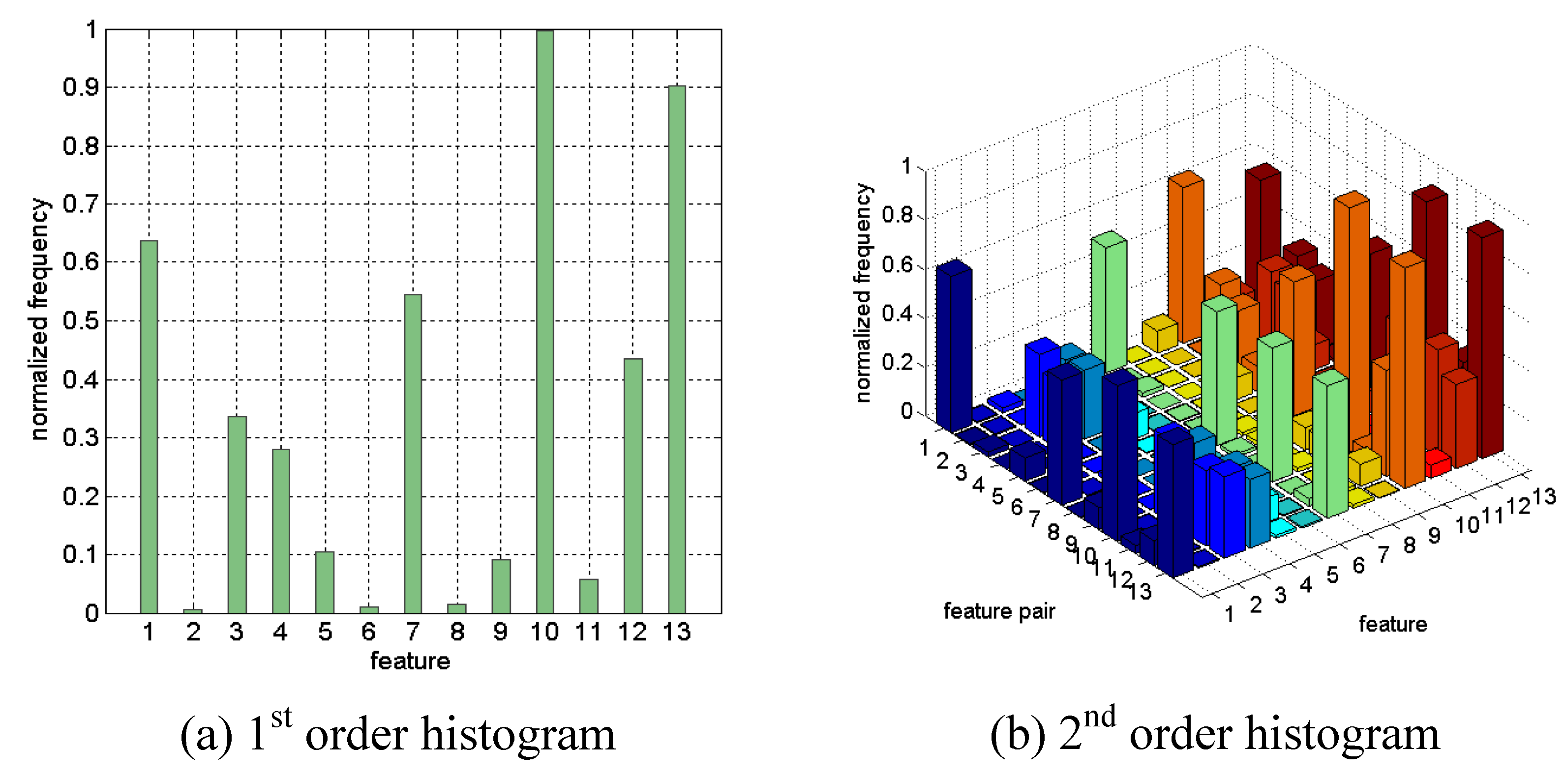
Figure 23 shows the first and second order histogram of Wine data achieved by 10 runs of the LOOFS. The k-NN voting classifier was used as the fitness function by manually setting of the parameter (k = 5). Table 10 gives the detail results of three approaches. The selection stability of eye image data is very low, which indicates that no specific strong feature is in the eye image data. The selected features really depend on the patterns included in the training set, which puts the reliability of the system into question. In addition to cross-validation techniques [16,26], the presented approach for stable feature selection tackles the general problem of specialization or overtraining, which is encountered in learning problems based on a limited number of examples. The experience gained for automated feature selection can be abstracted to other tasks and levels of the overall system design with the aspect of generating more stable and reliable systems. Again, the underlying effort must be traded-off with the expected performance and reliability gain. Thus, this extension is provided as an optional feature, that could be omitted if design speed and low design effort are more important.

Figure 23. First and second order statistics of Wine data.

Figure 23. First and second order statistics of Wine data.

Table 10. Results of selected features by HAF, ELRF, and NLF methods using k–NN voting classifier with k = 5.

Dataset	Sf	HAF		ELRF		NLF		Class (%)
		Class. (%)	Feature	Class. (%)	Feature	Class. (%)	Feature	Mean	Median
Wine	0.57	96.06	4	96.62	6	96.06	4	95.41	96.06
Rock	0.59	99.09	3	95.45	6	99.09	3	97.65	98.18
Eye image	0.09	96.24	7	99.24	22	97.74	17	96.77	96.99

Table 10. Results of selected features by HAF, ELRF, and NLF methods using k–NN voting classifier with k = 5.

Dataset	Sf	HAF		ELRF		NLF		Class (%)
		Class. (%)	Feature	Class. (%)	Feature	Class. (%)	Feature	Mean	Median
Wine	0.57	96.06	4	96.62	6	96.06	4	95.41	96.06
Rock	0.59	99.09	3	95.45	6	99.09	3	97.65	98.18
Eye image	0.09	96.24	7	99.24	22	97.74	17	96.77	96.99

7. Efficient Classifiers Optimization

In the final stage of the computational modelling shown in Figure 7, we describe the process of classifier optimisation. There are two main focuses in the classifier optimisation, i.e., to select the proper parameter of the classifier and to obtain lean but well performing classifier. The second focus is of particular relevance in mobile implementation due to imposed resource limitations.

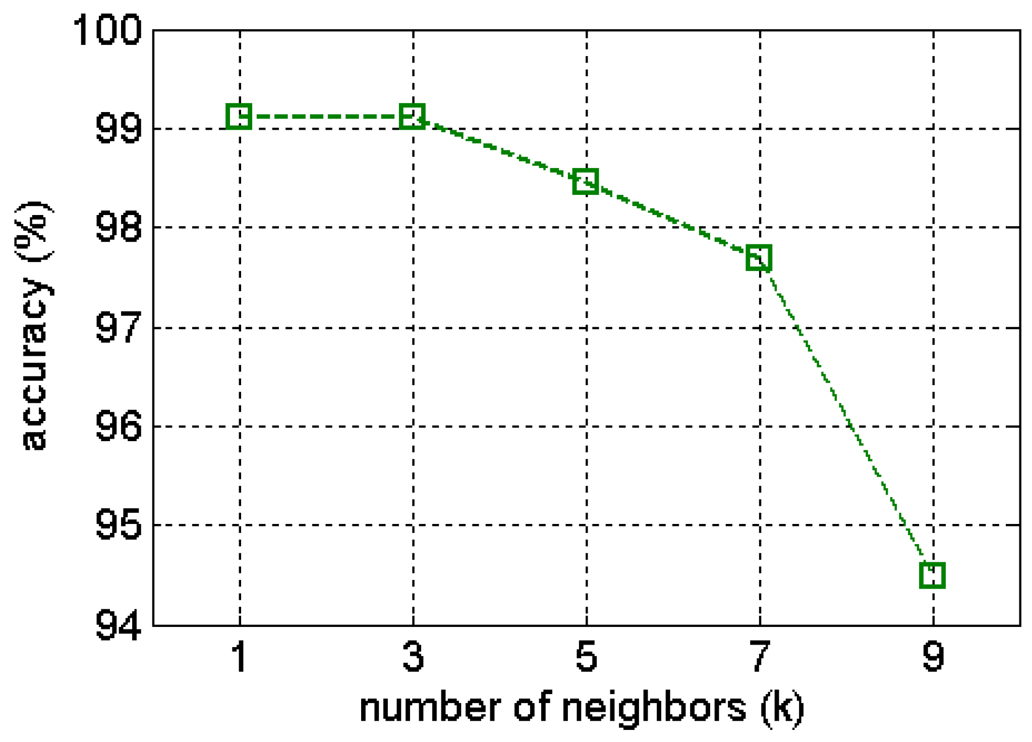
The parameters of classifiers play an important role for obtaining good results. For example, in the nearest neighbor classifier (k-NN), the sensitivity of k parameter has been investigated for the gas benchmark data as shown in Figure 24 [26]. In automated feature selection, employing a classifier as assessment function (wrapper method), the representation of candidate solutions of GA or PSO is extended by including the chosen classifier’s parameters along with the binary feature in the gene or particle during optimisation. Practically, this describes a special case of simultaneously co-evolving two steps of the design process, i.e. dimensionality reduction and classification [14].

Figure 24. Sensitivity investigation of k–NN using extracted features by Gaussian kernel (GWF) of gas benchmark data. The k parameter values are set as 1, 3, 5, 7, and 9.

Figure 24. Sensitivity investigation of k–NN using extracted features by Gaussian kernel (GWF) of gas benchmark data. The k parameter values are set as 1, 3, 5, 7, and 9.

Many classifiers, for instance, nearest neighbor (k-NN) and probabilistic neural networks (PNN), use the training set as prototypes to evaluate the new patterns. There are numerous related previous works focused on the designing lean classifiers, i.e., particularly resource-aware classifier instances. Hart proposed that pruning methods reduced the amount of data which has to be stored for the nearest neighbor classifier called Condensed Nearest Neighbor (CNN) [55]. Gates proposed a postprocessing step for the CNN pruning algorithm called Reduced Nearest Neighbor (RNN) [54]. The Restricted Coulomb Energy (RCE) is a three layer feedforward network, which gradually selects the prototypes in a only growing approach and adjusts their radii until satisfactory training. The limitations of CNN, RNN, and RCE methods are: (1) their result strongly depends on the presentation order of the training set and (2) prototypes are selected from training without any adjustment. The work of Platt introduced Resource-Allocating Networks (RAN), which are related to RCE and Radial Basis Function networks (RBF) [56]. The RAN method allows to insert new prototypes for of Gaussian kernels, which will be adjusted as well as their centers by gradient descent technique in training. This attractive method is hampered due to well-known gradient descent limitations. Improvements can be found, e.g., in Cervantes et al. [39], where a new algorithm for nearest neighbor classification called Adaptive Michigan PSO, which can obtain less number of prototypes and is able to adjust their positions is proposed. These adjusted prototypes using AMPSO can classify the new patterns better than CNN, RNN, and RCE. The manner of encoding of the Michigan PSO is much better suited to optimize the named classifiers’ structure than the standard PSO. Thus, the Michigan approach was chosen for our work. In [38], a novel adaptive resource-aware Probabilistic Neural Network (ARAPNN) model was investigated using Michigan-nested Pittsburgh PSO algorithms.

Original implementation of PSO and GA encodes one candidate solution (a particle for PSO or a chromosome for GA) as one complete solution of the problem. This is also known as Pittsburgh approach. In optimization algorithms based on Michigan approach, each individual of the population represents one of patterns (prototypes) selected from the training set and the population represents as a single solution. This particle representation has advantages compared with original PSO, where particles have lower dimension and less computational effort, also flexibility in growing and reducing the number of prototypes.

In the algorithm for optimizing the PNN classifier, the Michigan approach is placed as the main optimisation procedure, which is used for obtaining the best position of prototypes and adjusting the number of prototypes. The Pittsburgh approach embedded inside the main algorithm as nested optimization procedure is applied for obtaining the best smoothing factor (σ) of Gaussian distribution function, which regulates the density approximation. In the Michigan approach, each particle is interpreted as a single prototype with its class affiliation, which is defined as follows:

$$x_i=\left\{\langle x_{i,1},x_{i,2},\dots ,x_{i,d}\rangle ,\langle {\omega }_i\rangle \right\}$$

(35)

$$INFO=\left\{\langle float\rangle ,\langle none\rangle \right\}$$

(36)

where d denotes the number of variables or features, x_i is the i-th prototype, ω_i denotes the class information of the prototype. This class information does not evolve, but remains fixed for each particle. This is signed by ‘none’ in INFO variable. Each particle movement is evaluated by the local objective function, which measures its contribution in classifying new patterns with regard to the statistical value. Two additional operators included in the PSO algorithm of ARAPNN are reproduction and reduction of prototypes. These two operator are used to increase or decrease the number of prototypes. The whole swarm of particles is evaluated by global function, which is the classification rate of PNN. If the current global fitness larger than pervious one, then the current best swarm will be saved by replacing the old one. More detail description for this optimisation procedure of ARAPNN can be seen in [38]. Similar to this concept of the ARAPNN or AMAPSO algorithms, the basic algorithm of PSO and GA can be expanded or modified to deal with other classifiers.

Here, we show the feasibility of the optimization algorithm in our ADIMSS tool by performing experimentation on five sets of well-known benchmark data collected from the UCI Machine Learning Repository. Table 11 describes the parameter settings of ARAPNN used in the experiments. The parameters of the optimization algorithms are set manually by the expert designer. In the extension process of optimization loops, those parameters can be included in the automated searching process. Table 12 and Table 13 show the experimental results of five benchmark datasets. The ARAPNN achieves less prototypes than RNN and SVM. In the classification rates, the performance of ARAPNN are close to the SVM classifier, but shows better results compared to the performance achieved by RNN and standard PNN.

Table 11. The parameter settings of ARAPNN .

Population: 3 patterns per class randomly select as individuals wstart = 0.9; wend = 0.4 c1 = 0.35; c2 = 0.35; c3 = 0.1 Update fcn = floating-point Maximum generation = 50 Fitness fcn = local and global Data splitting = 60% - training and 40% - validation Repeat = 20 runs

Table 11. The parameter settings of ARAPNN .

Population: 3 patterns per class randomly select as individuals wstart = 0.9; wend = 0.4 c1 = 0.35; c2 = 0.35; c3 = 0.1 Update fcn = floating-point Maximum generation = 50 Fitness fcn = local and global Data splitting = 60% - training and 40% - validation Repeat = 20 runs

Table 12. Comparison of the averaged number of prototypes selected by RNN, SVM, and ARAPNN [38].

Method	Bupa	Diabetes	Wine	Thyroid	Glass
RNN	123.75	233.20	19.05	20.55	62.25
SVM	140.20	237.65	35.75	27.30	136.85
ARAPNN	41.05	166.45	18.85	12.40	28.24

Table 12. Comparison of the averaged number of prototypes selected by RNN, SVM, and ARAPNN [38].

Method	Bupa	Diabetes	Wine	Thyroid	Glass
RNN	123.75	233.20	19.05	20.55	62.25
SVM	140.20	237.65	35.75	27.30	136.85
ARAPNN	41.05	166.45	18.85	12.40	28.24

Table 13. Comparison of the averaged classification rates of RNN, SVM, standard PNN and ARAPNN [38].

Method	Bupa	Diabetes	Wine	Thyroid	Glass
RNN	59.06	65.64	93.24	94.65	64.71
SVM	66.67	75.91	96.90	96.57	68.13
PNN	62.93	73.92	95.14	95.87	66.10
ARAPNN	64.49	75.57	96.41	96.40	67.70

Table 13. Comparison of the averaged classification rates of RNN, SVM, standard PNN and ARAPNN [38].

Method	Bupa	Diabetes	Wine	Thyroid	Glass
RNN	59.06	65.64	93.24	94.65	64.71
SVM	66.67	75.91	96.90	96.57	68.13
PNN	62.93	73.92	95.14	95.87	66.10
ARAPNN	64.49	75.57	96.41	96.40	67.70

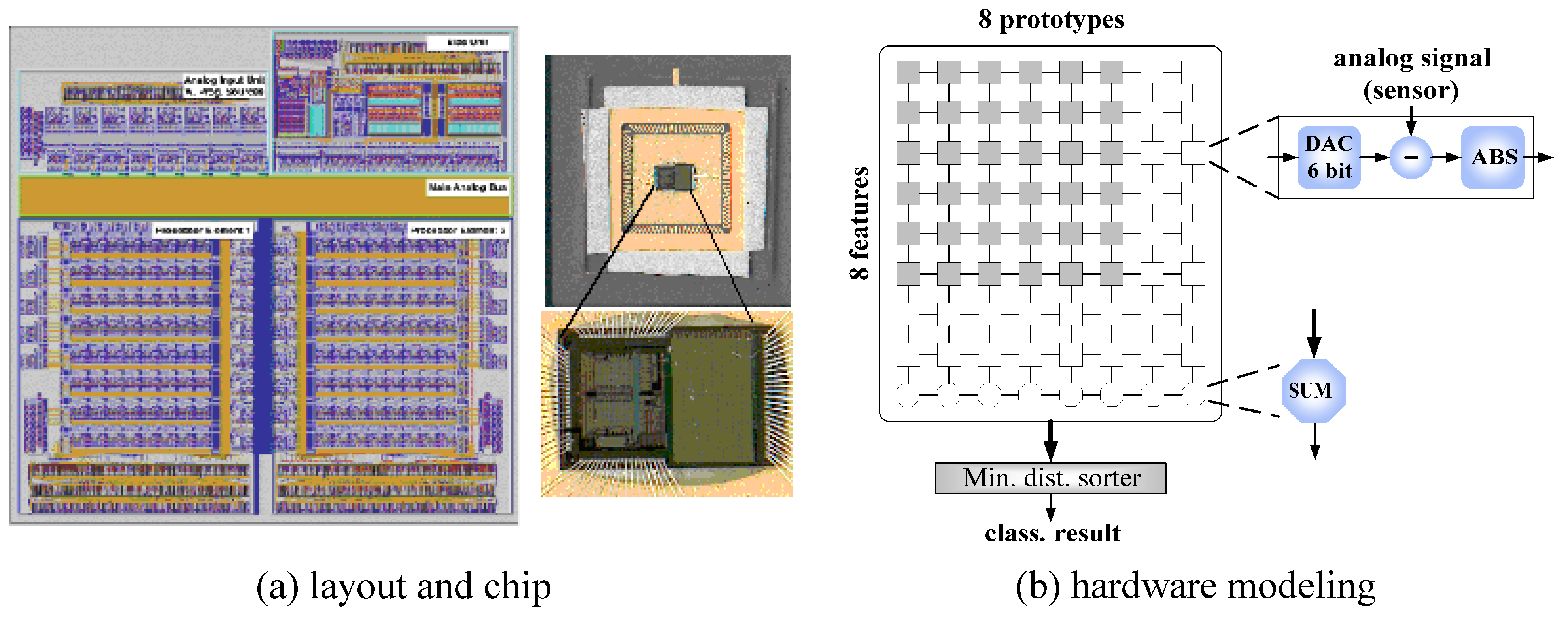
The proposed optimization scheme in our design architecture is demonstrated for the final classification block in extrinsic mode, i.e., based on the simulation of our classifier model. Extension to intrinsic mode, i.e., assuming a physical classifier hardware in the optimization loop as in evolvable hardware schemes [47], is discussed. In previous research work, a dedicated low–power 1–nearest–neighbor classifier has been designed in mixed–signal architecture in CMOS 0.6 μm technology. In our work, the statistical behavior and deviations were modelled as constraints in the extrinsic optimisation. A viable solution was evolved for the given classification problem and underlying electronic realization, optimizing the expected applicability or yield of implemented electronic instances [31]. The pursued approach can easily be extended to the intrinsic case by putting the chip instead of the statistical computational classifier model in the loop. Assessment during evolution is less demanding in this case of nonlinear decision making as for linear systems, e.g., sensor amplifiers [40,41]. To cope with the instance-specific deviations, basically obtained prototypes of the nearest neighbor classifier in the computational system model still have to be adjusted by the optimization algorithm with regard to these hardware constraints in the deployment time. Figure 25 shows the layout and chip of the classifier, designed in a previous research project, as well as the conceived corresponding computational hardware model of the 1–NN classifier, incorporating statistical features to model instance deviations.

Figure 25. Layout and chip of reconfigurable mixed-signal classifier chip and hardware modeling of nearest neighbor classifier.

Figure 25. Layout and chip of reconfigurable mixed-signal classifier chip and hardware modeling of nearest neighbor classifier.

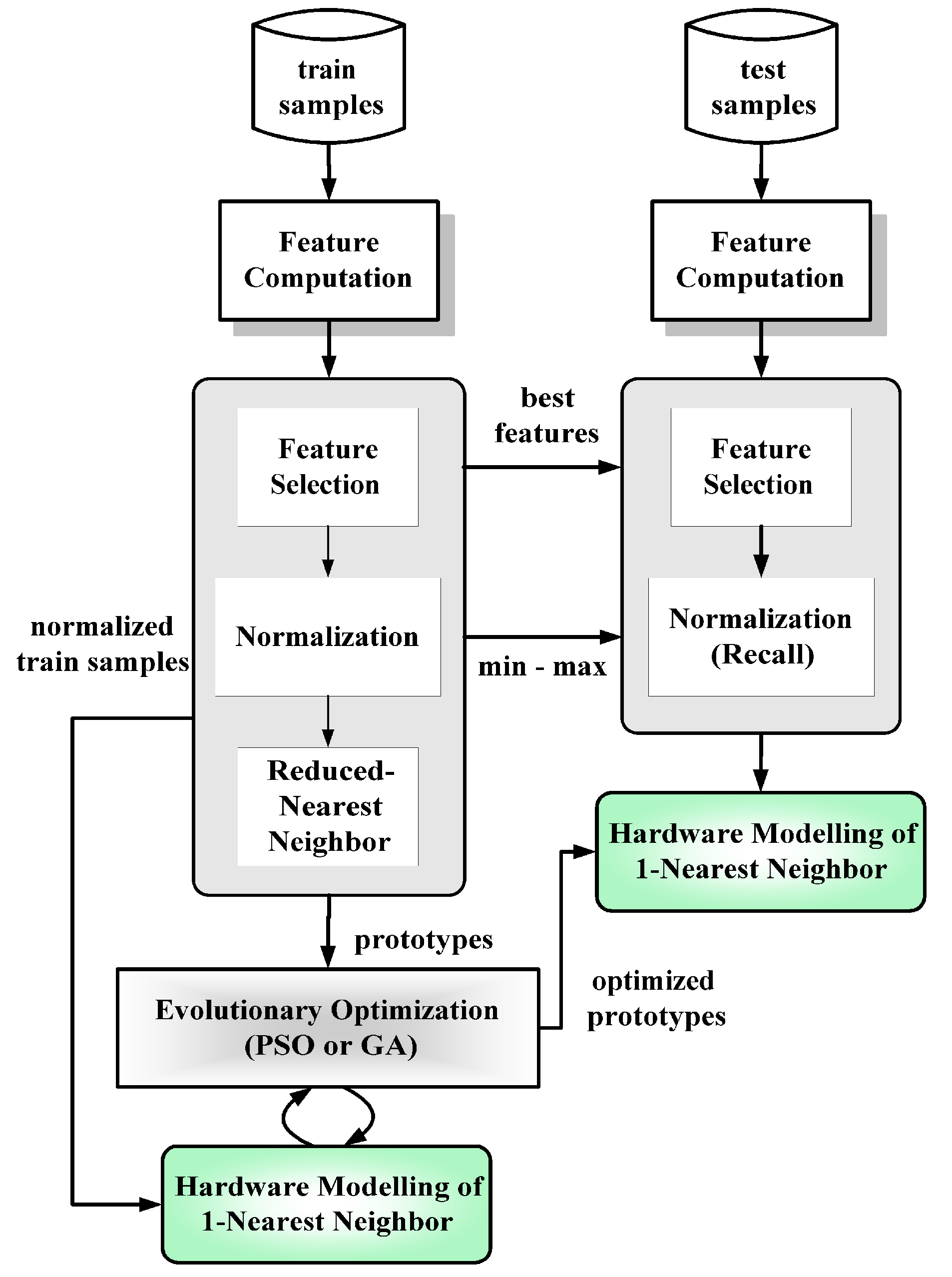
The current optimisation algorithm only adjusts the fixed number of prototypes prescribed by the initial problem solution. Adaptive increase of the prototype number to the limits of the available resources in case of unsatisfactory solution could be done in the next step. The procedure of the prototype optimization is shown in Figure 26.

Figure 26. Procedure of the hardware constraint prototype optimization.

Figure 26. Procedure of the hardware constraint prototype optimization.

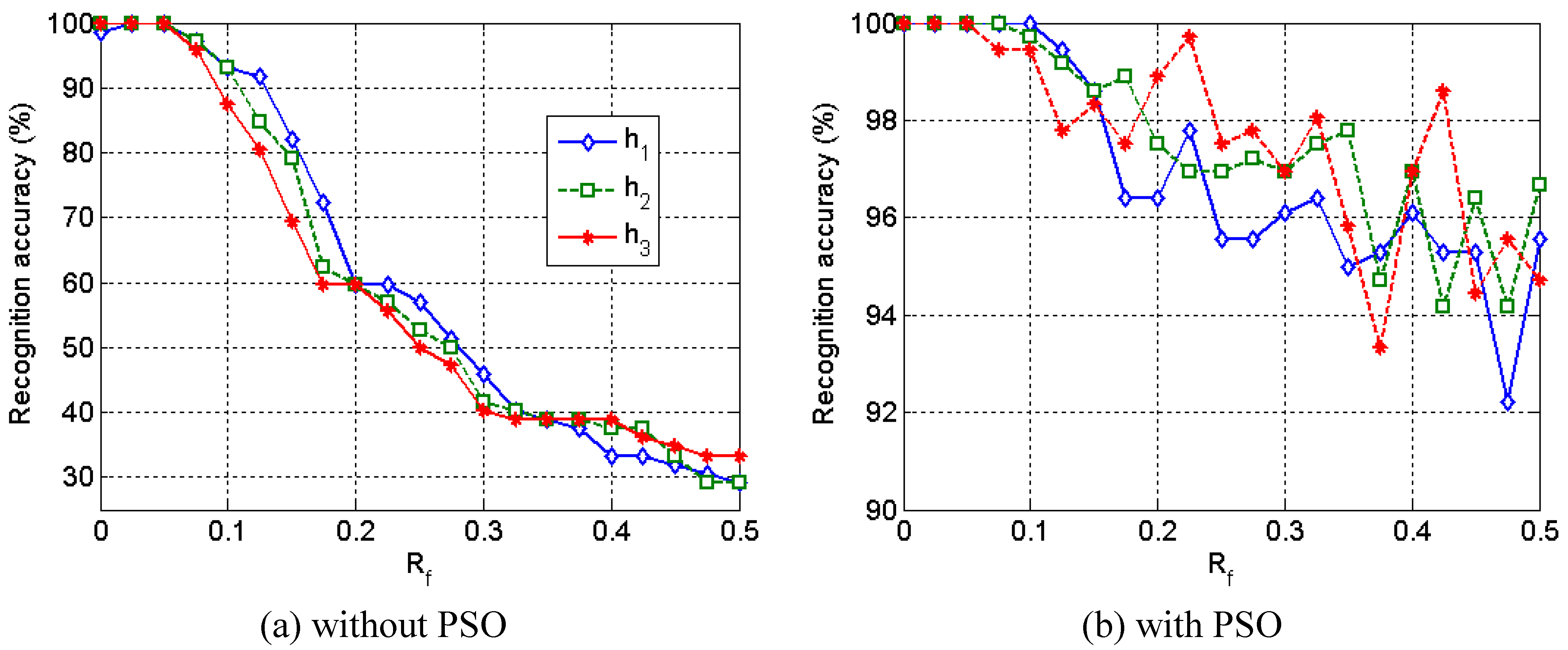
Figure 27 shows the experimental results between the adjusted prototypes by PSO and the prototypes which are not adjusted. The PSO algorithm has succeeded in effectively recovering the classifier performance regarding to classification accuracies, even for extreme deviations. However, it still cannot restore up to 100% of classification rates for high perturbation cases due to exhausted prototype resource, which can be tackle by adaptively increasing of the prototype number to the limits of available resources.

Figure 27. Classification accuracies on test set of eye image data, where h_i and R_f are perturbation factors in the computational hardware model [31].

Figure 27. Classification accuracies on test set of eye image data, where h_i and R_f are perturbation factors in the computational hardware model [31].

8. Conclusions

Our paper deals with a particular design automation approach to overcome a bottleneck in conceiving and implementing intelligent sensor systems. This bottleneck is aggravated by the rapid emergence of novel sensing elements, computing nodes, wireless communication and integration technology, which actually give unprecedented possibilities for intelligent systems design and application. To effectively exploit these possibilities, design methodology and related frameworks/tools for automated design are required. We summarized the few existing activities, predominantly found in the field of industrial vision. We have conceived a methodology, that takes into account the specificities of multi–sensor–systems and allows to incorporate multiple objectives and constraints of physical realization into a computational model and in a resource-aware design process.

The architecture and current implementation was demonstrated step by step employing gas sensor and benchmark data examples. It can be shown that competitive or superior solutions can be found and resource–constraints can be included in the design process. The method portfolio is currently extended and the potential design space reduction by employment of a priori knowledge is advanced.

We have also discussed the extension of the adaptive design architecture to deployment and operation time, where, based on appropriate reconfigurable hardware, self-x properties can be achieved by intrinsic evolution to achieve robust and well-performing self-x sensor intelligent systems.

A future extension of the group’s research work will be directed towards wireless-sensor-networks, where, in contrast to the lumped systems regarded so far, sensing and decision making is distributed and load distribution with regards to computation vs. communication in the context of intelligent systems. as well as potential occurrence of missing data must be treated. Corresponding extensions of the presented methodology and tool will be pursued.