Forecasting the Unit Cost of a Product with Some Linear Fuzzy Collaborative Forecasting Models

Department of Industrial Engineering and Systems Management, Feng Chia University, Taichung City, 407, Taiwan
Algorithms 2012, 5(4), 449-468; https://doi.org/10.3390/a5040449
Submission received: 6 June 2012
/
Revised: 7 September 2012
/
Accepted: 17 September 2012
/
Published: 15 October 2012
Abstract
:Forecasting the unit cost of every product type in a factory is an important task. However, it is not easy to deal with the uncertainty of the unit cost. Fuzzy collaborative forecasting is a very effective treatment of the uncertainty in the distributed environment. This paper presents some linear fuzzy collaborative forecasting models to predict the unit cost of a product. In these models, the experts’ forecasts differ and therefore need to be aggregated through collaboration. According to the experimental results, the effectiveness of forecasting the unit cost was considerably improved through collaboration.
1. Introduction
Cost forecasting means different things at different stages of the product life cycle. In product design, the designer needs to know whether the product will be economically produced. After a product goes into mass production, forecasting the unit cost is the basis of financial and production planning activities. When a product enters the market, the follow-up customer service and maintenance costs must also be taken into account.
Accurately predicting the unit cost of each product type is a very important task in any factory. If the unit cost is less than expected, then the efforts and investment of cost reduction are not necessary. Conversely, if the unit cost is more than expected, then the profitability of the product will be over-estimated, resulting in the wrong investment and production decisions. However, forecasting the unit cost is not an easy task because of the uncertainty of the unit cost, mainly due to the cost of human operations in the production of products, which is sometimes unstable. In addition, there is not much relevant literature in the unit cost forecasting. On the other hand, several recent studies (e.g. [1,2,3,4,5,6,7,8,9,10,11,12,13,14]) showed that fuzzy collaborative forecasting has great potential for the prediction of processes with uncertainty, such as yield learning, changes in price, fluctuations in the cycle time, and others. For these reasons, the application of fuzzy collaborative forecasting methods to improve the performance of the unit cost forecasting is worth a try. Therefore, some fuzzy collaborative forecasting models are proposed in this study, in order to enhance the accuracy and precision of the unit cost forecast.
In the proposed methodology, the stakeholders are a group of domain experts, such as the product engineer, factory managers and accounting department staff. These experts apply fuzzy linear regression methods to predict the unit cost of a product. A fuzzy linear regression equation can be converted into a linear or nonlinear programming problem in a variety of ways. Furthermore, within the conversion process some parameters need a subject setting. As a result, forecasts obtained by the experts may be very different and therefore requires a collaborative mechanism to deal with the following issues:
- (1) How to integrate these forecasts?
- (2) How experts can refer to the forecasts of others to modify their own?
In response to this issue, the methods presented in this study are as follows:
- (1) Some linear fuzzy regression models for the unit cost forecasting are proposed and compared.
- (2) Development of dedicated software to pass the forecast of each expert to other experts for their reference. In the meantime, the software can integrate different forecasts using the hybrid fuzzy intersection and back propagation network approach.
- (3) In reference to the forecasts of others, each expert subjectively modifies the parameters in the fuzzy linear regression method.
The objectives of this study are as follows:
- (1) To enhance the accuracy of the unit cost forecast. In other words, the forecasts obtained must be very close to the actual values.
- (2) To improve the precision of the unit cost forecasting. Namely, a very small range containing the actual value can be estimated.
- (3) The application of an instance to compare the advantages and disadvantages of different linear fuzzy collaborative forecasting models.
The organization of this study is described as follow. Section 2 first reviews the literature related to fuzzy collaborative forecasting and the unit cost forecasting. The problems faced by the existing methods are also discussed. Then, in Section 3, some fuzzy collaborative forecasting models are proposed to predict the unit cost of a product. An example is given to illustrate the applicability of these models. Section 4 makes conclusions and suggests some directions for future research.
2. Related Work
Carnes [15] established a basic equation to calculate the unit cost of a wafer. Carnes also compared the long-term costs of ownership of two alternative machines, but these costs were not allocated to the two machines. Wood [16] defined the lowest cost of all operations on the same machine as the minimum wafer cost. In Pfitzner et al.’s view, the recovery of wafers is becoming increasingly important in reducing the unit cost along with the growth in size of a wafer [17].
Although there have been some literature about fuzzy collaborative intelligence and systems, but very few directly related to fuzzy collaborative forecasting. Shai and Reich [18,19] defined the concept of infused design as an approach for establishing effective collaboration between designers from different engineering fields. Büyüközkan and Vardaloglu [20,21] applied the fuzzy cognitive map method to the collaborative planning, forecasting and replenishment of a supply chain. The initial values of the concepts and the connection weights of the fuzzy cognitive map are dependent on the subjective belief of the expert and can be modified after collaboration. According to Poler et al. [22], the comparison of collaboration methods and the proposing of software tools, especially as regards forecasting methods for collaborative forecasting, are still lacking. Pedrycz and Rai [14] discussed the problem of collaborative data analysis by a group of agents having access to different parts of data and exchanging findings through their collaboration. A two-phase optimization procedure was established, so that the results of communication can be embedded into the local optimization results. In recent years, Chen [6] used a hybrid fuzzy linear regression-back propagation network approach to predict the efficient cost per unit of a semiconductor product. This method first gathered a group of experts in the field. Each expert then used a fuzzy linear regression equation to predict the future unit cost. The result is a fuzzy value, and can be regarded as a non-symmetric interval forecast. A crisp forecast rarely equal to the actual value. In contrast, a fuzzy forecast can contain the actual value. The fuzzy forecasts obtained by different experts are aggregated using a fuzzy intersection, resulting in a polygon-shaped fuzzy number, which can be defuzzified using a back propagation network. Chen [4] considered the case in which each expert has only partial access to the data, and is not willing to share the raw data he/she owns. The forecasting results by an expert are conveyed to other experts for the modification of their settings, so that the actual values will be contained in the fuzzy forecasts after collaboration. All fuzzy collaborative intelligence methods seek consensus of results. In this field, Ostrosi et al. [23] defined the concept of consensus as the overlapping of design clusters of different perspectives. Similarly, Chen [2] defined the concept of partial consensus as the intersection of the views of some experts. Cheikhrouhou et al. [24] thought that collaboration is necessary because of the unexpected events that may occur in the future demand.
In short, the existing approaches have the following problems:
- (1) The unit cost forecasted by the existing methods may be lower than the actual value, resulting in over-estimated profits if the financial plan is based on the forecasts.
- (2) For precision in the unit cost forecasting, the narrowest scope containing the actual value is required; however, this has rarely been discussed.
- (3) The peak and average unit costs are forecasted separately, which is problematic because it is possible that the forecast becomes invalid in the sense that the average value may be higher than the peak value [10].
- (4) The existing fuzzy linear regression-back propagation network methods selected particular fuzzy linear regression methods, but did not explain the reasons or compared with other fuzzy linear regression methods.
3. Methodology
The parameters used in the proposed methodology are defined in advance.
- (1) b: learning constant.
- (2)
![Algorithms 05 00449 i001]() : normalized unit cost at period t.
: normalized unit cost at period t. - (3) ct: actual unit cost at period t.
- (4)
![Algorithms 05 00449 i002]() : fuzzy unit cost forecast at period t.
: fuzzy unit cost forecast at period t. ![Algorithms 05 00449 i003]() if it is represented with a triangular fuzzy number .
if it is represented with a triangular fuzzy number . - (5) C: unit wafer cost.
- (6) G: gross die.
- (7) r(t): homoscedastical, serially non-correlated error term.
- (8) t: period.
- (9) T: current period.
- (10) Yt: yield at period t.
- (11) Y0: asymptotic/final yield.


Prior to predict the unit cost of a product, we emphasize at the outset that the reduction in the unit cost follows a learning process, which is the assumption of this study.
3.1. Fuzzy Linear Regression Methods for Forecasting the Unit Cost
According to Gruber [25], the yield of a product follows a learning process:
![Algorithms 05 00449 i004]()

The unit cost can be calculated as
![Algorithms 05 00449 i005]() Obviously, the change in the unti cost is also a learning process, not a usual time-series. After converting to logarithms,
Obviously, the change in the unti cost is also a learning process, not a usual time-series. After converting to logarithms,
![Algorithms 05 00449 i006]() where a = lnC − lnY0 − lnG. To consider the uncertainty in the unit cost, parameters in equation (3) are given in asymmetric triangular fuzzy numbers as follows [26,27,28,29]:
where a = lnC − lnY0 − lnG. To consider the uncertainty in the unit cost, parameters in equation (3) are given in asymmetric triangular fuzzy numbers as follows [26,27,28,29]:
![Algorithms 05 00449 i007]()
![Algorithms 05 00449 i008]() Therefore,
Therefore,
![Algorithms 05 00449 i009]() where (+) represents fuzzy addition. Equation (6) is obviously a fuzzy linear regression equation.
where (+) represents fuzzy addition. Equation (6) is obviously a fuzzy linear regression equation.


A fuzzy linear regression equation can be fitted in various ways. For example, in Tanaka and Watada [30], a linear programming problem is solved to minimize the fuzziness:
![Algorithms 05 00449 i010]() subject to
subject to
![Algorithms 05 00449 i011]()
![Algorithms 05 00449 i012]()
![Algorithms 05 00449 i013]()
![Algorithms 05 00449 i014]()
![Algorithms 05 00449 i015]()
![Algorithms 05 00449 i016]()
![Algorithms 05 00449 i017]()
![Algorithms 05 00449 i018]() where s is the satisfaction level. For the training data, the actual values will fall within the ranges of the fuzzy forecasts. Clearly, the higher value of s leads to wider fuzzy forecasts. This model is indicated with WT(s).
where s is the satisfaction level. For the training data, the actual values will fall within the ranges of the fuzzy forecasts. Clearly, the higher value of s leads to wider fuzzy forecasts. This model is indicated with WT(s).


The second method for fitting a fuzzy linear regression equation is Peters’ method [31], in which the following linear programming problem is solved, aimed at the maximization of the average satisfaction level:
![Algorithms 05 00449 i019]() subject to
subject to
![Algorithms 05 00449 i020]()
![Algorithms 05 00449 i021]()
![Algorithms 05 00449 i022]()
![Algorithms 05 00449 i023]()
![Algorithms 05 00449 i024]()
![Algorithms 05 00449 i025]()
![Algorithms 05 00449 i026]()
![Algorithms 05 00449 i027]()
![Algorithms 05 00449 i028]()
![Algorithms 05 00449 i029]()
![Algorithms 05 00449 i030]() where d is the required range of a fuzzy forecast. Clearly, a larger value of d results in a higher average satisfaction level. This model is indicated with Peters(d).
where d is the required range of a fuzzy forecast. Clearly, a larger value of d results in a higher average satisfaction level. This model is indicated with Peters(d).


The third method for fitting a fuzzy linear regression equation is Donoso’s quadratic non-possibilistic method [32], in which the quadratic error for both the central tendency and each one of the spreads is minimized:
![Algorithms 05 00449 i031]() subject to
subject to
![Algorithms 05 00449 i065]()
![Algorithms 05 00449 i067]()
![Algorithms 05 00449 i069]()
![Algorithms 05 00449 i071]()
![Algorithms 05 00449 i073]()
![Algorithms 05 00449 i075]()
![Algorithms 05 00449 i077]()
![Algorithms 05 00449 i032]() where k1 and k2 belong to [0 1], and add up to 1. This model is indicated with Donoso(k1, k2, s).
where k1 and k2 belong to [0 1], and add up to 1. This model is indicated with Donoso(k1, k2, s).


The fourth method for fitting a fuzzy linear regression equation is Chen and Lin’s nonlinear programming method [8], which changes the objectives and constraints in the two linear programming models into nonlinear:
Model I
![Algorithms 05 00449 i033]() subject to
subject to
![Algorithms 05 00449 i066]()
![Algorithms 05 00449 i068]()
![Algorithms 05 00449 i070]()
![Algorithms 05 00449 i072]()
![Algorithms 05 00449 i074]()
![Algorithms 05 00449 i076]()
![Algorithms 05 00449 i078]()
![Algorithms 05 00449 i034]()


Model II
![Algorithms 05 00449 i035]() subject to
subject to
![Algorithms 05 00449 i036]()
![Algorithms 05 00449 i079]()
![Algorithms 05 00449 i080]()
![Algorithms 05 00449 i037]()
![Algorithms 05 00449 i081]()
![Algorithms 05 00449 i082]()
![Algorithms 05 00449 i083]()
![Algorithms 05 00449 i084]()
![Algorithms 05 00449 i085]()
![Algorithms 05 00449 i086]()
![Algorithms 05 00449 i038]() where o reflects the sensitivity to the uncertainty of the fuzzy forecast; o ranges from 0 (not sensitive) to ∞ (extremely sensitive); s indicates the required satisfaction level;
where o reflects the sensitivity to the uncertainty of the fuzzy forecast; o ranges from 0 (not sensitive) to ∞ (extremely sensitive); s indicates the required satisfaction level; ![Algorithms 05 00449 i039]() ; d is the desired range of every fuzzy forecast;
; d is the desired range of every fuzzy forecast; ![Algorithms 05 00449 i040]() ; m represents the relative importance of the outliers in fitting the fuzzy linear regression equation;
; m represents the relative importance of the outliers in fitting the fuzzy linear regression equation; ![Algorithms 05 00449 i041]() . When m = 1, the relative importance of the outliers is the highest and is equal to that of the non-outliers. o should be set within [0 1] if the variation in the variable is less than 1. Otherwise, it should be greater than 1. The two nonlinear programming models are indicated with CL1(o, s) and CL2(o, d, m), respectively.
. When m = 1, the relative importance of the outliers is the highest and is equal to that of the non-outliers. o should be set within [0 1] if the variation in the variable is less than 1. Otherwise, it should be greater than 1. The two nonlinear programming models are indicated with CL1(o, s) and CL2(o, d, m), respectively.


 ; d is the desired range of every fuzzy forecast;
  ; m represents the relative importance of the outliers in fitting the fuzzy linear regression equation;
  . When m = 1, the relative importance of the outliers is the highest and is equal to that of the non-outliers. o should be set within [0 1] if the variation in the variable is less than 1. Otherwise, it should be greater than 1. The two nonlinear programming models are indicated with CL1(o, s) and CL2(o, d, m), respectively.
3.2. Aggregation of Fuzzy Forecasts in Fuzzy Collaborative Forecasting
A mechanism is required to combine the fuzzy forecasts. The aggregation mechanism consists of two steps. In the first step, fuzzy intersection is applied to aggregate the fuzzy forecasts into a polygon-shaped fuzzy number, in order to improve the precision of forecasting. Every fuzzy forecast contains the actual value. As a result, the intersection of the fuzzy forecasts also contains the actual value. Besides, the intersection has a narrower range than those of the original regions. Therefore, the forecasting precision measured in terms of the average range is indeed improved after intersection, which is one of the basic mechanisms of fuzzy collaborative forecasting. Fuzzy intersection combines n fuzzy forecasts in the following manner:
![Algorithms 05 00449 i042]() where
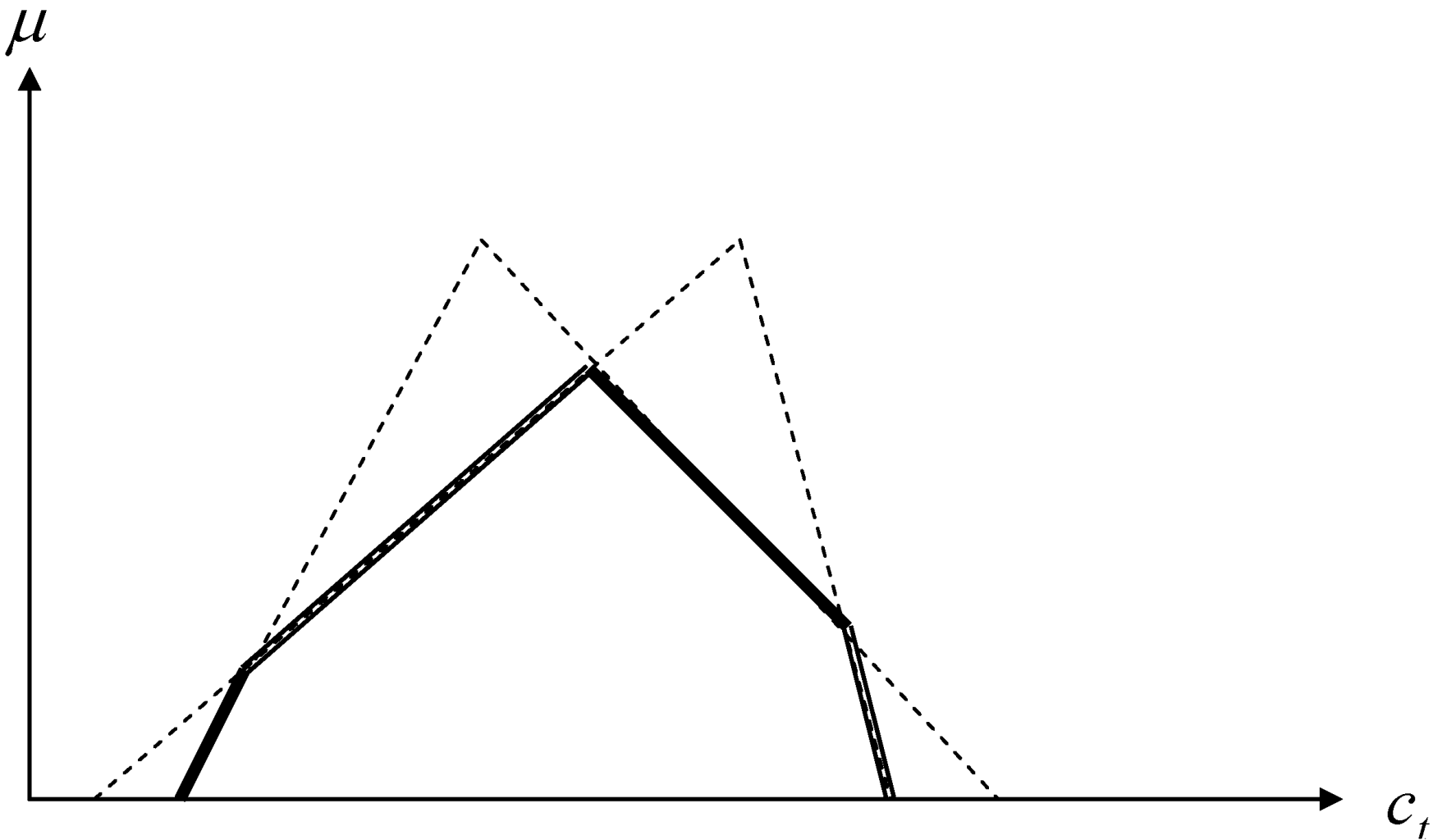
where ![Algorithms 05 00449 i043]() indicates the result of obtaining the fuzzy intersection of the fuzzy forecasts by L experts. If these fuzzy forecasts are approximated with triangular fuzzy numbers, then the fuzzy intersection is a polygon-shaped fuzzy number (see Figure 1).
indicates the result of obtaining the fuzzy intersection of the fuzzy forecasts by L experts. If these fuzzy forecasts are approximated with triangular fuzzy numbers, then the fuzzy intersection is a polygon-shaped fuzzy number (see Figure 1).

 indicates the result of obtaining the fuzzy intersection of the fuzzy forecasts by L experts. If these fuzzy forecasts are approximated with triangular fuzzy numbers, then the fuzzy intersection is a polygon-shaped fuzzy number (see Figure 1).
 Figure 1.
The fuzzy intersection of two triangular fuzzy numbers.
The result of this step is a polygon-shaped fuzzy number that specifies the narrowest range of the fuzzy forecast. However, in practical applications a crisp forecast is usually required. Therefore, a crisp forecast has to be generated from the polygon-shaped fuzzy number. For this purpose, a variety of defuzzification methods are applicable [33]. Once the defuzzified value is obtained it is compared with the actual value to evaluate the accuracy. However, among the existing defuzzification methods, no one method is better than all the other methods in every case. In addition, the most suitable defuzzification method for a fuzzy variable is often chosen from the existing methods, and thus the optimality of the chosen method cannot be guaranteed. Also, the shape of the polygon-shaped fuzzy number is special. These phenomena are reasons for proposing a tailored defuzzification method. In this study, a back propagation network is applied, because theoretically a well-trained back propagation network (without being stuck in a local minima) with a good selected topology can successfully map any complex distribution.
The configuration of the back propagation network used is established as follows:
- (1) Inputs: 2m parameters corresponding to the m corners of the polygon-shaped fuzzy number and the membership function values of these corners. The reason is that simple–aggregation results in a convex domain and each point in it can be expressed with the combination of corners. The fuzzy intersection of L fuzzy forecasts will have at most 2·(2L + 2) corners. All input parameters have to be normalized into a range narrower than [0 1] before they are fed into the network.
- (2) Single hidden layer: Generally one or two hidden layers are more beneficial for the convergence property of the back propagation network.
- (3) The number of neurons in the hidden layer is chosen from 1~4m according to a preliminary analysis, considering both effectiveness (forecasting accuracy) and efficiency (execution time).
- (4) Output: the crisp forecast.
- (5) Network learning rule: Delta rule.
- (6) Network learning algorithms: There are many advanced algorithms for training a back propagation network, e.g. the Fletcher–Reeves algorithm, the Broydon–Fletcher–Goldfarb–Shanno algorithm, the Levenberg–Marquardt algorithm, and the Bayesian regularization method [34]. In this study, the Levenberg-Marquardt algorithm is applied.
- (7) Number of epochs per replication: 10,000.
- (8) Activation function: Log-sigmoid function.
- (9) Number of initial conditions/replications: Because the performance of a back propagation network is sensitive to the initial condition, the training process will be repeated many times with different initial conditions that are randomly generated. Among the results, the best one is chosen for the subsequent analyses.
The Levenberg-Marquardt algorithm was designed for training with second-order speed without having to compute the Hessian matrix. It uses approximation and updates the network parameters in a Newton-like way. When training a back propagation network, the Hessian matrix can be approximated as:
![Algorithms 05 00449 i045]() and the gradient can be computed as:
and the gradient can be computed as:
![Algorithms 05 00449 i046]() where J is the Jacobian matrix containing the first derivatives of the network errors with respect to the weights and biases; e is the vector of the network errors. The Levenberg-Marquardt algorithm uses this approximation and updates the network parameters in a Newton-like way:
where J is the Jacobian matrix containing the first derivatives of the network errors with respect to the weights and biases; e is the vector of the network errors. The Levenberg-Marquardt algorithm uses this approximation and updates the network parameters in a Newton-like way:
![Algorithms 05 00449 i047]() where ep is the epoch number. Newton’s method is faster and more accurate near an error minimum, so the Levenberg-Marquardt algorithm’s purpose is to move as quickly as possible to Newton’s method. Thus, μ decreases after each successful step and increases only when a tentative step will increase the performance function. Consequently, the performance function is always reduced after each epoch.
where ep is the epoch number. Newton’s method is faster and more accurate near an error minimum, so the Levenberg-Marquardt algorithm’s purpose is to move as quickly as possible to Newton’s method. Thus, μ decreases after each successful step and increases only when a tentative step will increase the performance function. Consequently, the performance function is always reduced after each epoch.


3.3. Performance Evaluation in Fuzzy Collaborative Forecasting
Some performance measures of fuzzy collaborative forecasting are defined as follows.
Definition 1. F(p) is a fuzzy forecasting method with parameter p. The fuzzy forecast at period t using F(p) is indicated with ![Algorithms 05 00449 i048]() . The precision and accuracy of F(p) are indicated with Prec(F(p)) and Accur(F(p)), respectively. Some of the common functions for Prec(F(p)) and Accur(F(p)) are described below:
. The precision and accuracy of F(p) are indicated with Prec(F(p)) and Accur(F(p)), respectively. Some of the common functions for Prec(F(p)) and Accur(F(p)) are described below:
 . The precision and accuracy of F(p) are indicated with Prec(F(p)) and Accur(F(p)), respectively. Some of the common functions for Prec(F(p)) and Accur(F(p)) are described below:
(1) The average range (AR):
![Algorithms 05 00449 i049]()
![Algorithms 05 00449 i050]()
![Algorithms 05 00449 i051]() where D() is the defuzzification function;
where D() is the defuzzification function; ![Algorithms 05 00449 i052]() is the actual value at period t.
is the actual value at period t.


 is the actual value at period t.
Mean absolute percentage error (MAPE):
![Algorithms 05 00449 i053]()

(2) Root mean squared error (RMSE):
![Algorithms 05 00449 i054]() All of these performance indicators are as small as possible.
All of these performance indicators are as small as possible.

Definition 2. FCF(F, G) is a fuzzy collaborative forecasting method on the basis of two forecasting methods F and G. The quality of collaboration in the precision and accuracy are indicated with QoCp(FCF) and QoCa(FCF), respectively. Some of the common functions for QoCp(FCF) and QoCa(FCF) are described below:
(1) Maximum percentage improvement (MPI):
![Algorithms 05 00449 i055]()
![Algorithms 05 00449 i056]()


(2) Average percentage improvement (API):
![Algorithms 05 00449 i057]()
![Algorithms 05 00449 i058]()


These functions can easily be extended to involve more than two objects.
3.4. Some Fuzzy Collaborative Forecasting Models for the Unit Cost Forecasting
An example is given in Table 1. The data of the first 7 periods were used as training data, and the remaining data are left for testing.

| t | ct (US$) |
|---|---|
| 1 | 2.57 |
| 2 | 1.61 |
| 3 | 1.76 |
| 4 | 1.28 |
| 5 | 1.53 |
| 6 | 1.19 |
| 7 | 1.32 |
| 8 | 1.32 |
| 9 | 1.61 |
| 10 | 1.32 |
Some linear fuzzy collaboration forecasting models for used to predict the unit cost.
Model 1. FCF(WT(s1), WT(s2))
In this model, the two objects use the same fuzzy linear regression method (WT(s)), but with different values of s to predict the unit cost. In WT(s), the most precise forecast is associated with the minimum value of s that satisfies the constraints. In addition, the results when s is large often contain the results when s is relatively small, which makes it less effective for their collaboration. Nevertheless, the fuzzy collaborative forecasting method, to a certain extent, improves the precision of WT(s). In the previous example, assuming the s values specified by the objects are 0.3 and 0.6, respectively:
- PrecAR(WT(0.3)) = 0.56
- PrecAR(WT(0.6)) = 1.14
- PrecAR(FCF(WT(0.3), WT(0.6))) = 0.53
Therefore, the quality of collaboration with respect to the forecasting precision can be evaluated as
- QoCpMPI,AR(FCF(WT(0.3), WT(0.6))) = max((1.14 − 0.53)/1.14, (0.56 − 0.53)/0.56) = 54%.
- QoCpAPI,AR(FCF(WT(0.3), WT(0.6))) = ((1.14 − 0.53)/1.14 + (0.56 − 0.53)/0.56)/2 = 29%.
In order to evaluate the forecasting accuracy, the forecasts by the two objects are defuzzified using the center of gravity (COG) method, and then are compared with the actual values:
- AccuMAE(WT(0.3)) = 0.16
- AccuMAE(WT(0.6)) = 0.24
- AccuMAPE(WT(0.3)) = 10%
- AccuMAPE(WT(0.6)) = 15%
- AccuRMSE(WT(0.3)) = 0.19
- AccuRMSE(WT(0.6)) = 0.31
while in the fuzzy collaborative forecasting method, the forecasts by the two objects are aggregated using the fuzzy intersection and back propagation network approach to generate a single crisp value:
- AccuMAE(FCF(WT(0.3), WT(0.6))) = 0.06
- AccuMAPE(FCF(WT(0.3), WT(0.6))) = 4%
- AccuRMSE(FCF(WT(0.3), WT(0.6))) = 0.10
Therefore, the quality of collaboration with respect tothe forecasting accuracy can be evaluated as
- QoCaMPI,MAE(FCF(WT(0.3), WT(0.6))) = max((0.16 − 0.07)/0.16, (0.24 − 0.07)/0.24) = 71%.
- QoCaAPI,MAE(FCF(WT(0.3), WT(0.6))) = ((0.16 − 0.07)/0.16 + (0.24 − 0.07)/0.24)/2 = 64%.
- QoCaMPI,MAPE(FCF(WT(0.3), WT(0.6))) = max((10% − 5%)/10%, (15% − 5%)/15%) = 67%.
- QoCaAPI,MAPE(FCF(WT(0.3), WT(0.6))) = ((10% − 5%)/10% + (15% − 5%)/15%)/2 = 58%.
- QoCaMPI,RMSE(FCF(WT(0.3), WT(0.6))) = max((0.19 − 0.15)/0.19, (0.31 − 0.15)/0.31) = 52%.
- QoCaAPI,RMSE(FCF(WT(0.3), WT(0.6))) = ((0.19 − 0.15)/0.19 + (0.31 − 0.15)/0.31)/2 = 36%.
Model 2. FCF(Peters(d1), Peters(d2))
In this model, both objects use Peters(d), but with different d values to predict the unit cost. In Peters(d), the most precise forecast is associated with the minimum value of d that satisfies the constraints. In addition, the results when d is large often contain the results when d is relatively small. As a result, the benefits of collaboration are not obvious. In the previous example, assuming the d values specified by the objects are 0.3 and 0.5, respectively. The forecasting performances of the two objects are evaluated as
- PrecAR(Peters(0.3)) = 0.48
- PrecAR(Peters(0.5)) = 0.68
- AccuMAE(Peters(0.3)) = 0.16
- AccuMAE(Peters(0.5)) = 0.20
- AccuMAPE(Peters(0.3)) = 10%
- AccuMAPE(Peters(0.5)) = 12%
- AccuRMSE(Peters(0.3)) = 0.19
- AccuRMSE(Peters(0.5)) = 0.25
After collaboration, the forecasting precision and accuracy are both improved:
- PrecAR(FCF(Peters(0.3), Peters(0.5))) = 0.48
- AccuMAE(FCF(Peters(0.3), Peters(0.5))) = 0.07
- AccuMAPE(FCF(Peters(0.3), Peters(0.5))) = 6%
- AccuRMSE(FCF(Peters(0.3), Peters(0.5))) = 0.13
The quality of collaboration in the two aspects can be evaluated as
- QoCpMPI,AR(FCF(Peters(0.3), Peters(0.5))) = 29%.
- QoCpAPI,AR(FCF(Peters(0.3), Peters(0.5))) = 15%.
and
- QoCaMPI,MAE(FCF(Peters(0.3), Peters(0.5))) = 65%.
- QoCaAPI,MAE(FCF(Peters(0.3), Peters(0.5))) = 61%.
- QoCaMPI,MAPE(FCF(Peters(0.3), Peters(0.5))) = 50%.
- QoCaAPI,MAPE(FCF(Peters(0.3), Peters(0.5))) = 45%.
- QoCaMPI,RMSE(FCF(Peters(0.3), Peters(0.5))) = 48%.
- QoCaAPI,RMSE(FCF(Peters(0.3), Peters(0.5))) = 40%.
respectively.
Model 3. FCF(Donoso(k11, k21, s1), Donoso(k12, k22, s2))
In this model, both objects use Donoso(k1, k2, s), but with different parameter values to predict the unit cost. This method has more parameters that can be adjusted, so there is a greater degree of freedom, which provides a space for coordination. Assuming in the previous example, the parameter values specified by the two objects are
- (k11, k21, s1) = (0.2, 0.8, 0.2)
- (k12, k22, s2) = (0.7, 0.3, 0.3)
Then their forecasting performances are
- PrecAR(Donoso(0.2, 0.8, 0.2)) = 0.48
- PrecAR(Donoso(0.7, 0.3, 0.3)) = 0.57
- AccuMAE(Donoso(0.2, 0.8, 0.2)) = 0.15
- AccuMAE(Donoso(0.7, 0.3, 0.3)) = 0.14
- AccuMAPE(Donoso(0.2, 0.8, 0.2)) = 9%
- AccuMAPE(Donoso(0.7, 0.3, 0.3)) = 9%
- AccuRMSE(Donoso(0.2, 0.8, 0.2)) = 0.17
- AccuRMSE(Donoso(0.7, 0.3, 0.3)) = 0.18
Comparatively, the forecasting performance of the fuzzy collaborative forecasting method is
- PrecAR(FCF(Donoso(0.2, 0.8, 0.2), Donoso(0.7, 0.3, 0.3))) = 0.48
- AccuMAE(FCF(Donoso(0.2, 0.8, 0.2), Donoso(0.7, 0.3, 0.3))) = 0.07
- AccuMAPE(FCF(Donoso(0.2, 0.8, 0.2), Donoso(0.7, 0.3, 0.3))) = 5%
- AccuRMSE(FCF(Donoso(0.2, 0.8, 0.2), Donoso(0.7, 0.3, 0.3))) = 0.10
Therefore, the quality of collaboration can be evaluated as
- QoCpMPI,AR(FCF(Donoso(0.2, 0.8, 0.2), Donoso(0.7, 0.3, 0.3)))) = 16%.
- QoCpAPI,AR(FCF(Donoso(0.2, 0.8, 0.2), Donoso(0.7, 0.3, 0.3)))) = 8%.
- QoCaMPI,MAE(FCF(Donoso(0.2, 0.8, 0.2), Donoso(0.7, 0.3, 0.3)))) = 53%.
- QoCaAPI,MAE(FCF(Donoso(0.2, 0.8, 0.2), Donoso(0.7, 0.3, 0.3)))) = 52%.
- QoCaMPI,MAPE(FCF(Donoso(0.2, 0.8, 0.2), Donoso(0.7, 0.3, 0.3)))) = 44%.
- QoCaAPI,MAPE(FCF(Donoso(0.2, 0.8, 0.2), Donoso(0.7, 0.3, 0.3)))) = 44%.
- QoCaMPI,RMSE(FCF(Donoso(0.2, 0.8, 0.2), Donoso(0.7, 0.3, 0.3)))) = 44%.
- QoCaAPI,RMSE(FCF(Donoso(0.2, 0.8, 0.2), Donoso(0.7, 0.3, 0.3)))) = 43%.
It is worth noting that the performance of this collaboration model is not as good as expected.
Model 4. FCF(CL1(o1, s1), CL1(o2, s2))
In this model, the two objects use the same method CL1(o, s), but with different values of o and s to predict the unit cost. CL1(o, s) is an extension of WT(s) by considering a nonlinear objective function instead. To make a comparison, the parameter values of the two objects are set to
- (o1, s1) = (3, 0.3)
- (o2, s2) = (2, 0.6)
The s values are the same with those in the original WT(s) methods. After forecasting the unit cost, the performances of the two objects are evaluated as
- PrecAR(CL1(3, 0.3)) = 0.56
- PrecAR(CL1(2, 0.6)) = 1.12
- AccuMAE(CL1(3, 0.3)) = 0.16
- AccuMAE(CL1(2, 0.6)) = 0.23
- AccuMAPE(CL1(3, 0.3)) = 10%
- AccuMAPE(CL1(2, 0.6))) = 14%
- AccuRMSE(CL1(3, 0.3)) = 0.19
- AccuRMSE(CL1(2, 0.6)) = 0.30
Then, the forecasting performances are compared with those of the linear methods WT(0.3) and WT(0.6). The results are summarized in Table 2.
| PrecAR | AccuMAE | AccuMAPE | AccuRMSE | |
|---|---|---|---|---|
| WT(0.3) | 0.56 | 0.16 | 0.1 | 0.19 |
| CL1(3, 0.3) | 0.56 | 0.16 | 0.1 | 0.19 |
| WT(0.6) | 1.14 | 0.24 | 0.15 | 0.31 |
| CL1(2, 0.6) | 1.12 | 0.23 | 0.14 | 0.3 |
Obviously, the use of a nonlinear objective function may change the optimal solution. The quality of collaboration is evaluated as follows:
- QoCpMPI,AR(FCF(CL1(3, 0.3), CL1(2, 0.6))) = 50%.
- QoCpAPI,AR(FCF(CL1(3, 0.3), CL1(2, 0.6))) = 25%.
- QoCaMPI,MAE(FCF(CL1(3, 0.3), CL1(2, 0.6))) = 71%.
- QoCaAPI,MAE(FCF(CL1(3, 0.3), CL1(2, 0.6))) = 65%.
- QoCaMPI,MAPE(FCF(CL1(3, 0.3), CL1(2, 0.6))) = 67%.
- QoCaAPI,MAPE(FCF(CL1(3, 0.3), CL1(2, 0.6))) = 60%.
- QoCaMPI,RMSE(FCF(CL1(3, 0.3), CL1(2, 0.6))) = 66%.
- QoCaAPI,RMSE(FCF(CL1(3, 0.3), CL1(2, 0.6))) = 57%.
Then, the quality of collaboration in FCF(CL1(3, 0.3), CL1(2, 0.6)) is compared with that in FCF(WT(0.3), WT(0.6)). The results are shown in Table 3.
| FCF(WT(0.3), WT(0.6)) | FCF(CL1(3, 0.3), CL1(2, 0.6)) | |
|---|---|---|
| QoCpMPI,AR | 54% | 50% |
| QoCpAPI,AR | 29% | 25% |
| QoCaMPI,MAE | 71% | 71% |
| QoCaAPI,MAE | 64% | 65% |
| QoCaMPI,MAPE | 67% | 67% |
| QoCaAPI,MAPE | 58% | 60% |
| QoCaMPI,RMSE | 52% | 66% |
| QoCaAPI,RMSE | 36% | 57% |
As can be seen from this table, the use of a nonlinear model CL1(o, s) instead of the linear model WT(s) can indeed achieve a better quality of collaboration, especially in the forecasting accuracy.
Model 5. FCF(CL2(o1, d1, m1), CL2(o2, d2, m2))
This model assumes that both of the two objects use CL2(o, d, m), but with different values to predict the unit cost
- (o1, d1, m1) = (3, 0.3, 2)
- (o2, d2, m2) = (2, 0.5, 3)
The performances of the two objects are evaluated as
- PrecAR(CL2(3, 0.3, 2)) = 0.48
- PrecAR(CL2(2, 0.5, 3)) = 0.66
- AccuMAE(CL2(3, 0.3, 2)) = 0.16
- AccuMAE(CL2(2, 0.5, 3)) = 0.16
- AccuMAPE(CL2(3, 0.3, 2)) = 10%
- AccuMAPE(CL2(2, 0.5, 3))) = 10%
- AccuRMSE(CL2(3, 0.3, 2)) = 0.19
- AccuRMSE(CL2(2, 0.5, 3)) = 0.20
Through the collaboration of the two objects, FCF(CL2(3, 0.3, 2), CL2(2, 0.5, 3)) achieves a better forecasting performance:
- PrecAR(FCF(CL2(3, 0.3, 2), CL2(2, 0.5, 3))) = 0.35
- AccuMAE(FCF(CL2(3, 0.3, 2), CL2(2, 0.5, 3))) = 0.05
- AccuMAPE(FCF(CL2(3, 0.3, 2), CL2(2, 0.5, 3))) = 4%
- AccuRMSE(FCF(CL2(3, 0.3, 2), CL2(2, 0.5, 3))) = 0.09
The quality of collaboration is assessed as follows:
- QoCpMPI,AR(FCF(CL2(3, 0.3, 2), CL2(2, 0.5, 3))) = 46%.
- QoCpAPI,AR(FCF(CL2(3, 0.3, 2), CL2(2, 0.5, 3))) = 37%.
- QoCaMPI,MAE(FCF(CL2(3, 0.3, 2), CL2(2, 0.5, 3))) = 69%.
- QoCaAPI,MAE(FCF(CL2(3, 0.3, 2), CL2(2, 0.5, 3))) = 68%.
- QoCaMPI,MAPE(FCF(CL2(3, 0.3, 2), CL2(2, 0.5, 3))) = 63%.
- QoCaAPI,MAPE(FCF(CL2(3, 0.3, 2), CL2(2, 0.5, 3))) = 63%.
- QoCaMPI,RMSE(FCF(CL2(3, 0.3, 2), CL2(2, 0.5, 3))) = 54%.
- QoCaAPI,RMSE(FCF(CL2(3, 0.3, 2), CL2(2, 0.5, 3))) = 53%.
Model 6. FCF(CL1(o1, s1), CL2(o2, d2, m2))
In this model, one of the two objects uses CL1(o, s), and the other uses CL2(o, d, m).
- (o1, s1) = (3, 0.3)
- (o2, d2, m2) = (2, 0.5, 3)
The forecasting performance of FCF(CL1(3, 0.3), CL2(2, 0.5, 3)) is evaluated as
- PrecAR(FCF(CL1(3, 0.3), CL2(2, 0.5, 3))) = 0.39
- AccuMAE(FCF(CL1(3, 0.3), CL2(2, 0.5, 3))) = 0.07
- AccuMAPE(FCF(CL1(3, 0.3), CL2(2, 0.5, 3))) = 5%
- AccuRMSE(FCF(CL1(3, 0.3), CL2(2, 0.5, 3))) = 0.11
The quality of collaboration is assessed as follows:
- QoCpMPI,AR(FCF(CL1(3, 0.3), CL2(2, 0.5, 3))) = 41%.
- QoCpAPI,AR(FCF(CL1(3, 0.3), CL2(2, 0.5, 3))) = 30%.
- QoCaMPI,MAE(FCF(CL1(3, 0.3), CL2(2, 0.5, 3))) = 59%.
- QoCaAPI,MAE(FCF(CL1(3, 0.3), CL2(2, 0.5, 3))) = 59%.
- QoCaMPI,MAPE(FCF(CL1(3, 0.3), CL2(2, 0.5, 3))) = 52%.
- QoCaAPI,MAPE(FCF(CL1(3, 0.3), CL2(2, 0.5, 3))) = 52%.
- QoCaMPI,RMSE(FCF(CL1(3, 0.3), CL2(2, 0.5, 3))) = 46%.
- QoCaAPI,RMSE(FCF(CL1(3, 0.3), CL2(2, 0.5, 3))) = 45%.
3.5. Comparison of the Performances of the Fuzzy Collaborative Forecasting Models
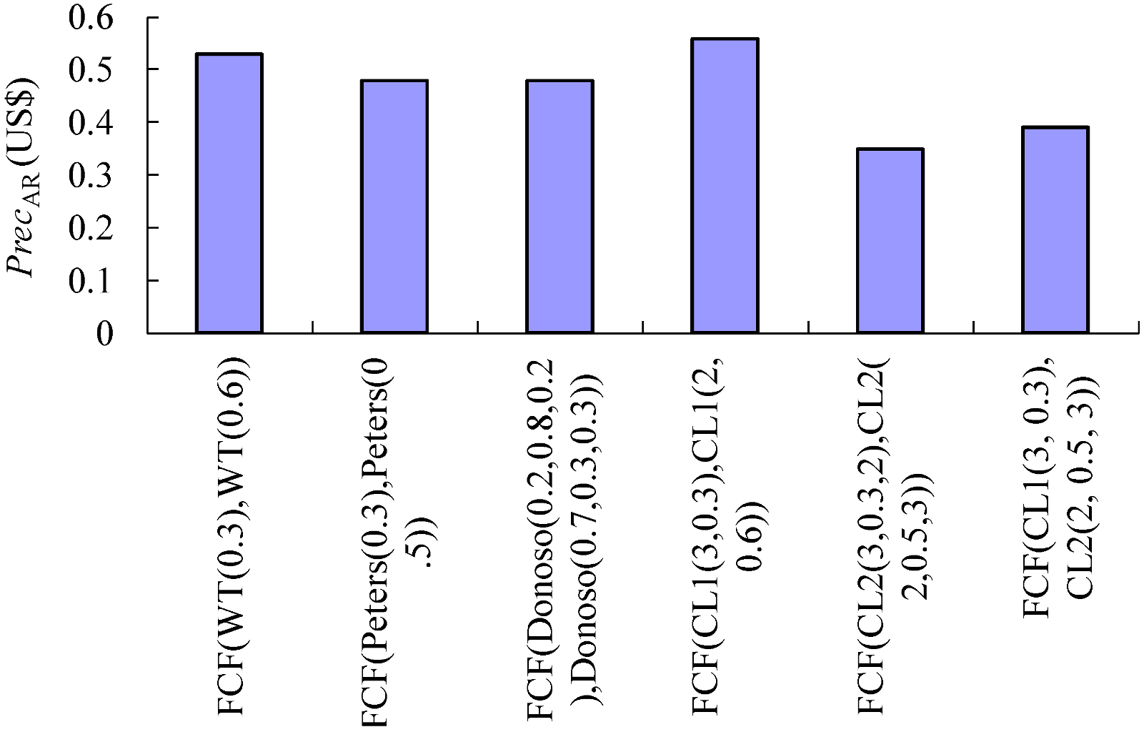
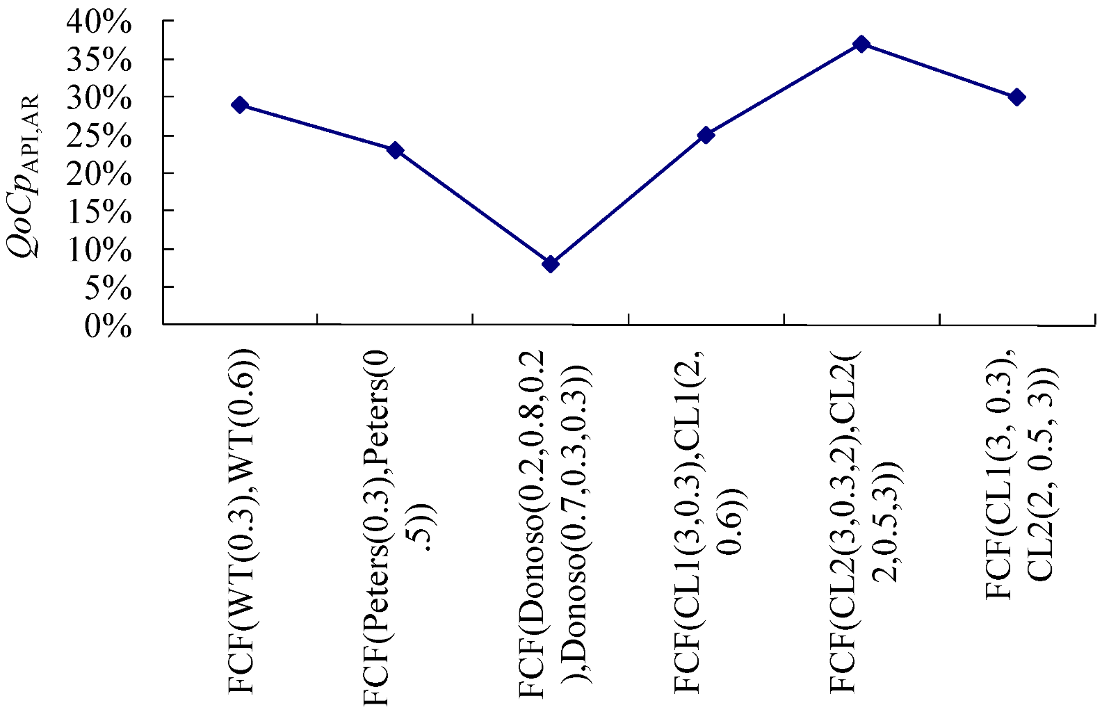
In this section, the performances of the fuzzy collaborative forecasting models are compared. First, the forecasting accuracy considering the average range of forecasts, the performances of different models are compared in Figure 2. Obviously, in terms of the forecasting accuracy, FCF(CL2(3, 0.3, 2), CL2(2, 0.5, 3)) is much better than the other models. However, this is partly because the settings of the parameters in the models are different and subjective. In order to confirm the effects of different models for the forecasting accuracy, the quality of collaboration, especially QoCpAPI,AR, is considered to be a better indicator. The comparison results are shown in Figure 3. As can be seen from this figure, FCF(CL2(3, 0.3, 2), CL2(2, 0.5, 3)) is indeed the most precise fuzzy collaborative forecasting model in this case.
Figure 2.
The forecasting accuracy of the fuzzy collaborative forecasting models.

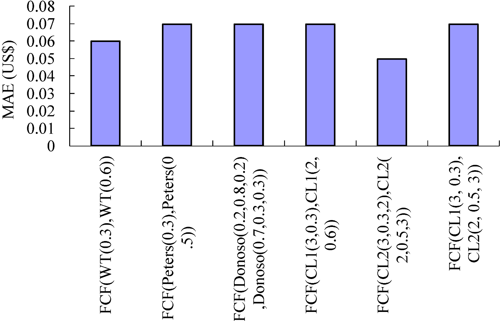
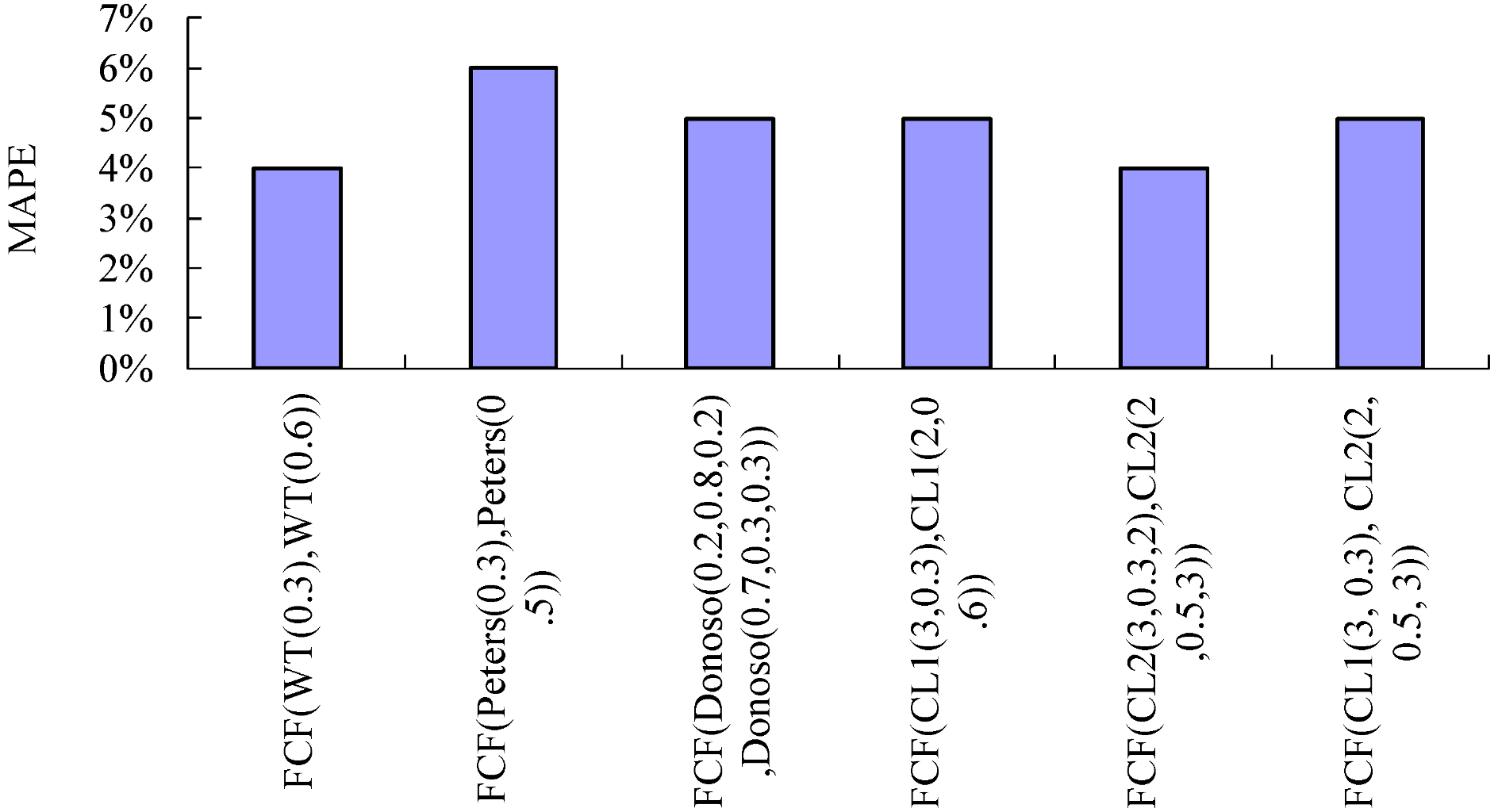
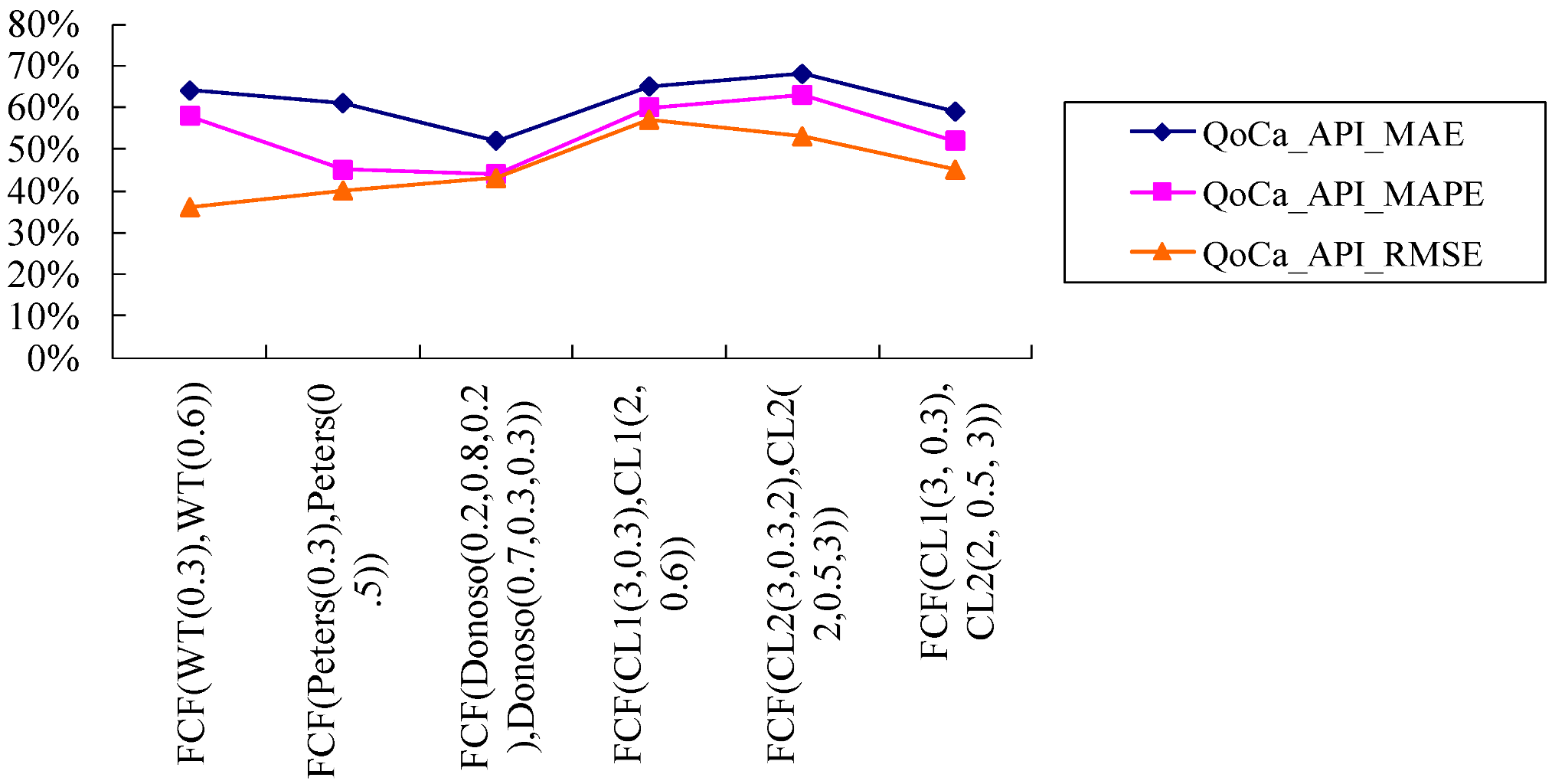
Secondly, in order to compare the forecasting accuracy of the models, three indicators—MAE, MAPE, and RMSE are considered. The comparison results in the three indicators are shown in Figure 4, Figure 5 and Figure 6, respectively. For all indicators of the forecasting accuracy, FCF(CL2(3, 0.3, 2), CL2(2, 0.5, 3)) is the best fuzzy collaborative forecasting model. Next, the quality of collaboration is compared, and the results are shown in Figure 7. The quality of collaboration in FCF(CL1(3, 0.3), CL1(2, 0.6)) is the best if RMSE is taken into account, and FCF(CL2(3, 0.3, 2), CL2(2, 0.5, 3)) achieves the highest quality of collaboration if MAE or MAPE is considered.
Figure 3.
The quality of collaboration of the fuzzy collaborative forecasting models.

Figure 4.
The forecasting accuracy (MAE) of the fuzzy collaborative forecasting models.

Figure 5.
The forecasting accuracy (MAPE) of the fuzzy collaborative forecasting models.

Figure 6.
The forecasting accuracy (RMSE) of the fuzzy collaborative forecasting models.
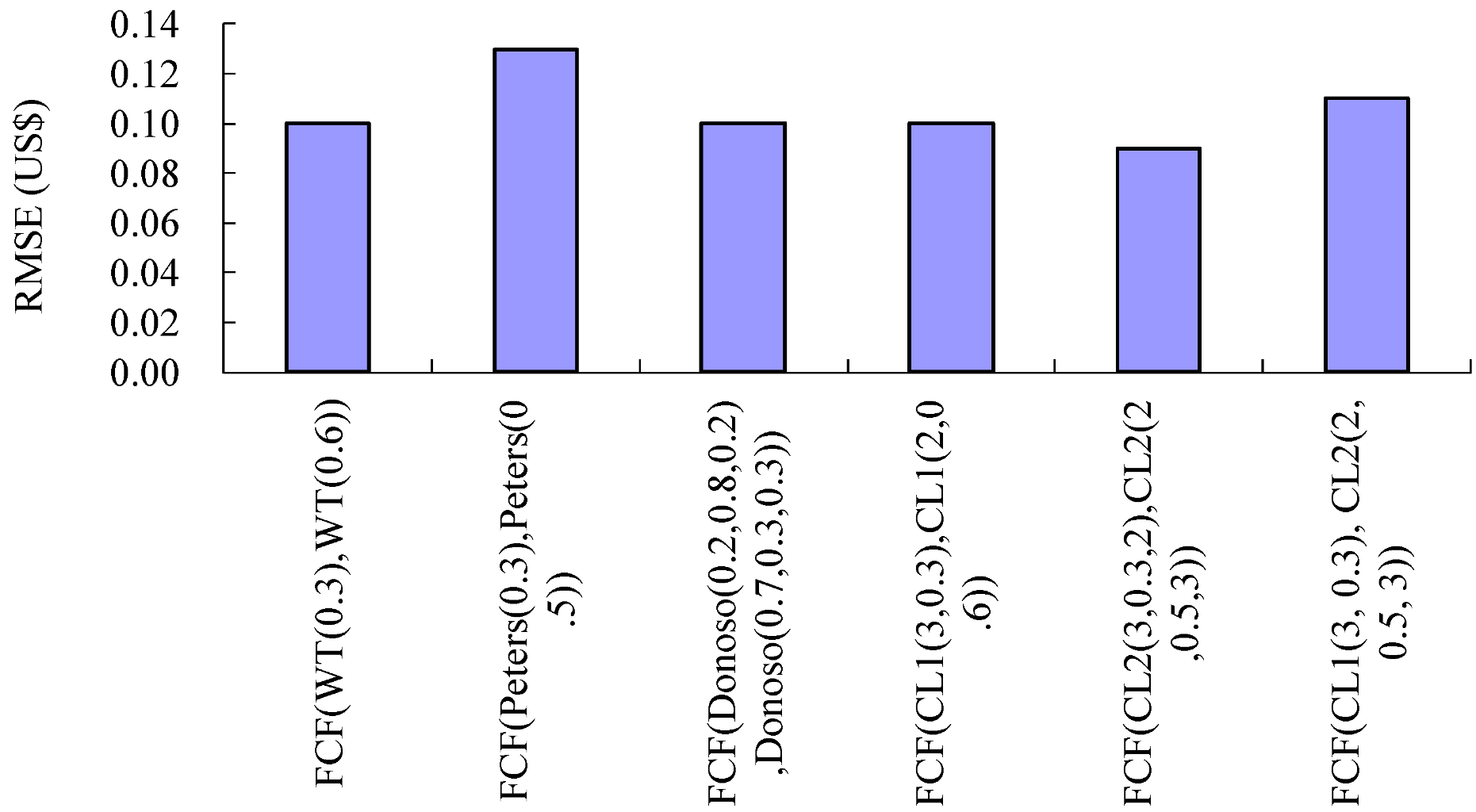
Figure 7.
The quality of collaboration of the fuzzy collaborative forecasting models.
4. Conclusions
Forecasting the unit cost of every product type in a factory is an important task. After the unit cost of every product type in a factory is accurately forecasted, several managerial goals (including pricing, cost down projecting, capacity planning, ordering decision support, and guiding subsequent operations) can be simultaneously achieved. However, it is not easy to deal with uncertainty in the unit cost. This paper presents some fuzzy collaborative forecasting models based on a few well-known fuzzy linear regression methods to predict the unit cost of a product. An example is used to illustrate the applicability of the proposed methodology. According to the experimental results,
- (1) The effectiveness of the unit cost forecasting was greatly improved through the collaboration of the experts, especially when using FCF(CL2(o1, d1, m1), CL2(o2, d2, m2)).
- (2) With respect to the quality of collaboration on the forecasting precision, only one performance measure is proposed and the proposed performance measure can effectively compare the differences among the models.
- (3) With respect to the forecasting accuracy on the forecasting accuracy among the performance measures, the one that considers MAPE can effectively compare the differences among the models.
The contribution of this study includes the following:
- (1) Six fuzzy collaborative forecasting models for the unit cost forecasting are investigated. From this, the most effective one can be identified.
- (2) More performance measures on the quality of collaboration have been proposed.
Acknowledgements
This work is partially supported by National Science Council of Taiwan.
References
- Chen, T. A fuzzy-neural knowledge-based system for job completion time prediction and internal due date assignment in a wafer fabrication plant. Int. J. Sys. Sci. 2009, 40, 889–902. [Google Scholar]
- Chen, T. A hybrid fuzzy and neural approach with virtual experts and partial consensus for DRAM price forecasting. Int. J. Innov. Comput. Inf. Control 2012, 8, 583–598. [Google Scholar]
- Chen, T. An online collaborative semiconductor yield forecasting system. Expert Sys. Appl. 2009, 36, 5830–5843. [Google Scholar] [CrossRef]
- Chen, T. An application of fuzzy collaborative intelligence to unit cost forecasting with partial data access by security consideration. Int. J. Technol. Intel. Plan. 2011, 7, 201–214. [Google Scholar] [CrossRef]
- Chen, T. Applying a fuzzy and neural approach for forecasting the foreign exchange rate. Int. J. Fuzzy Sys. Appl. 2011, 1, 36–48. [Google Scholar] [CrossRef]
- Chen, T. Applying the hybrid fuzzy c means-back propagation network approach to forecast the effective cost per die of a semiconductor product. Comput. Ind. Eng. 2011, 61, 752–759. [Google Scholar] [CrossRef]
- Chen, T. Some linear fuzzy collaborative forecasting models for semiconductor unit cost forecasting. Int. J. of Fuzzy Sys. Appl. 2012, in press. [Google Scholar]
- Chen, T.; Lin, Y.C. A fuzzy-neural system incorporating unequally important expert opinions for semiconductor yield forecasting. Int. J. Uncertain. Fuzziness Knowl. Based Syst. 2008, 16, 35–58. [Google Scholar] [CrossRef]
- Chen, T.; Lin, C.W.; Wang, Y.C. A fuzzy collaborative forecasting approach for WIP level estimation in a wafer fabrication factory. Appl. Math. Inf. Sci. 2012, in press. [Google Scholar]
- Chen, T.; Wang, Y.C. A fuzzy-neural approach for global CO2 concentration forecasting. Intel. Data Anal. 2011, 15, 763–777. [Google Scholar]
- Chen, T.; Wang, Y.C. A hybrid fuzzy and neural approach for forecasting the book-to-bill ratio in the semiconductor manufacturing industry. Int. J. Adv. Manuf. Technol. 2011, 54, 377–389. [Google Scholar] [CrossRef]
- Pedrycz, W. Collaborative architectures of fuzzy modeling. Lect. Notes Comput. Sci. 2008, 5050, 117–139. [Google Scholar]
- Pedrycz, W. Collaborative fuzzy clustering. Pattern Recognit. Lett. 2002, 23, 1675–1686. [Google Scholar]
- Pedrycz, W.; Rai, P. A multifaceted perspective at data analysis: A study in collaborative intelligent agents. IEEE Trans. Syst., Man. Cybern., Part B: Cybern. 2008, 38, 1062–1072. [Google Scholar] [CrossRef]
- Carnes, R. Long-term cost of ownership: beyond purchase price. In Proceedings of 1991 IEEE/SEMI International Semiconductor Science Symposium, Burlingame, CA, USA, 20-22 May 1991; pp. 39–43.
- Wood, S.C. Cost and cycle time performance of fabs based on integrated single-wafer processing. IEEE Trans. Semi. Manuf. 1997, 10, 98–111. [Google Scholar] [CrossRef]
- Pfitzner, L.; Benesch, N.; Öchsner, R.; Schmidt, C.; Schneider, C.; Tschaftary, T.; Trunk, R.; Dudenhausen, H.M. Cost reduction strategies for wafer expenditure. Microelectr. Eng. 2001, 56, 61–71. [Google Scholar] [CrossRef]
- Shai, O.; Reich, Y. Infused design I. Theory. Res. Eng. Design Res. 2004, 15, 93–107. [Google Scholar]
- Shai, O.; Reich, Y. Infused design II. Practice. Res. Eng. Design Res. 2004, 15, 108–121. [Google Scholar]
- Büyüközkan, G.; Vardaloglu, Z. Analyzing of Collaborative Planning, Forecasting and Replenishment Approachusing Fuzzy Cognitive Map. In Proceeding of 2009 International Conference on Computers and Industrial Engineering, University of Technology of Troyes, France, 6–8 July 2009; pp. 1751–1756.
- Büyüközkan, G.; Feyzioglu, O.; Vardaloglu, Z. Analyzing CPFR supporting factors with fuzzy cognitive map approach. World Academy Sci. Eng. Technol. 2009, 31, 412–417. [Google Scholar]
- Poler, R.; Hernandez, J.E.; Mula, J.; Lario, F.C. Collaborative forecasting in networked manufacturing enterprises. J. Manuf. Technol. Manag. 2008, 19, 514–528. [Google Scholar] [CrossRef]
- Ostrosi, E.; Haxhiaj, L.; Fukuda, S. Fuzzy modelling of consensus during design conflict resolution. Res. Eng. Design 2012, 23(1), 53–70. [Google Scholar]
- Cheikhrouhou, N.; Marmier, F.; Ayadi, O.; Wieser, P. A collaborative demand forecasting process with event-based fuzzy judgements. Comput. Ind. Eng. 2011, 61, 409–421. [Google Scholar] [CrossRef]
- Gruber, H. Learning and Strategic Product Innovation: Theory and Evidence for the Semiconductor Industry; Elsevier: Amsterdam, the Netherlands, 1994. [Google Scholar]
- Chen, T. A fuzzy back propagation network for output time prediction in a wafer fab. Appl. Soft Comput. 2003, 2, 211–222. [Google Scholar] [CrossRef]
- Chen, T. A hybrid fuzzy and neural approach for evaluating the cost competitiveness of a semiconductor product. Int. J. Technol. Intel. Plan. 2010, 6, 373–386. [Google Scholar] [CrossRef]
- Chen, T. A SOM-FBPN-ensemble approach with error feedback to adjust classification for wafer-lot completion time prediction. Int. J. Adv. Manuf. Technol. 2008, 37, 782–792. [Google Scholar] [CrossRef]
- Chen, T.; Wang, M.J.J. A fuzzy set approach for yield learning modeling in wafer manufacturing. IEEE Trans. Semicond. Manuf. 1999, 12, 252–258. [Google Scholar] [CrossRef]
- Tanaka, H.; Watada, J. Possibilistic linear systems and their application to the linear regression model. Fuzzy Sets Syst. 1988, 272, 275–289. [Google Scholar] [CrossRef]
- Peters, G. Fuzzy linear regression with fuzzy intervals. Fuzzy Sets Syst. 1994, 63, 45–55. [Google Scholar] [CrossRef]
- Donoso, S.; Marin, N.; Vila, M.A. Quadratic programming models for fuzzy regression. In Proceedings of International Conference on Mathematical and Statistical Modeling in Honor of Enrique Castillo, Ciudad Real, Spain, 28–30 June 2006.
- Liu, X. Parameterized defuzzification with maximum entropy weighting function—another view of the weighting function expectation method. Math. Com. Mod. 2007, 45, 177–188. [Google Scholar] [CrossRef]
- Eraslan, E. The estimation of product standard time by artificial neural networks in the molding industry. Math. Probl. Eng. 2009. article ID 527452. [Google Scholar]
© 2012 by the authors; licensee MDPI, Basel, Switzerland. This article is an open-access article distributed under the terms and conditions of the Creative Commons Attribution license (http://creativecommons.org/licenses/by/3.0/).
Share and Cite
MDPI and ACS Style
Chen, T. Forecasting the Unit Cost of a Product with Some Linear Fuzzy Collaborative Forecasting Models. Algorithms 2012, 5, 449-468. https://doi.org/10.3390/a5040449
AMA Style
Chen T. Forecasting the Unit Cost of a Product with Some Linear Fuzzy Collaborative Forecasting Models. Algorithms. 2012; 5(4):449-468. https://doi.org/10.3390/a5040449
Chicago/Turabian StyleChen, Toly. 2012. "Forecasting the Unit Cost of a Product with Some Linear Fuzzy Collaborative Forecasting Models" Algorithms 5, no. 4: 449-468. https://doi.org/10.3390/a5040449