Computing the Eccentricity Distribution of Large Graphs

Leiden Institute of Advanced Computer Science, Leiden University, P.O. Box 9512, 2300 RA Leiden, The Netherlands
*
Author to whom correspondence should be addressed.
Algorithms 2013, 6(1), 100-118; https://doi.org/10.3390/a6010100
Submission received: 1 November 2012
/
Revised: 24 January 2013
/
Accepted: 31 January 2013
/
Published: 18 February 2013
(This article belongs to the Special Issue Graph Algorithms)
Abstract
:The eccentricity of a node in a graph is defined as the length of a longest shortest path starting at that node. The eccentricity distribution over all nodes is a relevant descriptive property of the graph, and its extreme values allow the derivation of measures such as the radius, diameter, center and periphery of the graph. This paper describes two new methods for computing the eccentricity distribution of large graphs such as social networks, web graphs, biological networks and routing networks. We first propose an exact algorithm based on eccentricity lower and upper bounds, which achieves significant speedups compared to the straightforward algorithm when computing both the extreme values of the distribution as well as the eccentricity distribution as a whole. The second algorithm that we describe is a hybrid strategy that combines the exact approach with an efficient sampling technique in order to obtain an even larger speedup on the computation of the entire eccentricity distribution. We perform an extensive set of experiments on a number of large graphs in order to measure and compare the performance of our algorithms, and demonstrate how we can efficiently compute the eccentricity distribution of various large real-world graphs.
1. Introduction
Within the field of graph mining, researchers are often interested in deriving properties that describe the structure of their graphs. One of these properties is the eccentricity distribution, which describes the distribution of the eccentricity over all nodes, where the eccentricity of a node refers to the length of a longest shortest path starting at that node. This distribution differs from properties such as the distance distribution in the sense that eccentricity can be seen as a more “extreme” measure of distance. It also differs from indicators such as the degree distribution in the sense that determining the eccentricity of every node in the graph is computationally expensive: the traditional method computes the eccentricity of each node by running an All Pairs Shortest Path (APSP) algorithm, requiring time for a graph with n nodes and m edges. Unfortunately, this approach is too time-consuming if we consider large graphs with possibly millions of nodes.
The aforementioned complexity issues are frequently solved by determining the eccentricity of a random subset of the nodes in the original graph, and then deriving the eccentricity distribution from the obtained values [1]. While such an estimate may seem reasonable when the goal is to determine the overall average eccentricity value, we will show that this technique does not perform well when the actual extreme values of the distribution are of relevance. The nodes with the highest eccentricity values realize the diameter of the graph and form the so-called graph periphery, whereas the nodes with the lowest values realize the radius and form the center of the graph, and finding exactly these nodes can be useful within various application areas.
In routing networks, for example, it is interesting to know exactly which nodes form the periphery of the network and thus have the highest worst-case response time to any other device [2]. Also, when (routing) networks are modeled, for example for research purposes, it is important to measure the exact eccentricity distribution so that the model can be evaluated by comparing it with the distribution of real routing networks [3]. The eccentricity also plays a role in networks that model some biological system. There, proteins (nodes in the network) that have a low eccentricity value are easily functionally reachable by other components of the network [4]. The diameter, defined as the length of a longest shortest path, is the most frequently studied eccentricity-based measure, and efficient algorithms for its computation have been suggested in [5,6,7].
Generally speaking, the eccentricity can be seen as an extreme measure of centrality, i.e., the relative importance of a node in a graph. Centroid centrality [8] and graph centrality [9] have been suggested as centrality measures based on the eccentricity of a node. Compared to other measures such as closeness centrality, the main difference is that a node with a very low eccentricity value is relatively close to every other node, whereas a node with a low closeness centrality value is close to all the other nodes on average.
In this paper we first discuss an algorithm based on eccentricity lower and upper bounds for determining the exact eccentricity of every node of a graph. We also present a useful pruning strategy, and show how our method significantly improves upon the traditional algorithm. To realize an even larger speedup, we propose to incorporate a sampling technique on a specific set of nodes in the graph which allows us to obtain the eccentricity distribution much faster, while still ensuring a high accuracy on the eccentricity distribution, and an exact result for the eccentricity-based graph properties such as the radius and diameter.
The rest of this paper is organized as follows. We consider some notation and formulate the main problems addressed in this paper in Section 2, after which we cover related work in Section 3. Section 4 describes an exact algorithm for determining the eccentricity distribution. In Section 5, we explain how sampling can be incorporated. Results of applying our methods to various large datasets are presented in Section 6, and finally Section 7 summarizes the paper and offers suggestions for future work.
2. Preliminaries
We consider graphs , where V is the set of vertices (nodes) and is the set of edges (also called arcs or links). The distance between two nodes is defined as the length of a shortest path from v to w, i.e., the minimum number of edges that have to be traversed to get from v to w. We assume that our graphs are undirected, meaning that iff and thus for all . Note that each edge is thus included twice in E: once as a link from v to w and once as a link from w to v. We will also assume that G is connected, meaning that is always finite. Furthermore it is assumed that there are no parallel edges and no loops linking a node to itself. The neighborhood of a node v is defined as the set of all nodes connected to v via an edge: . The degree of a node v can then be defined as the number of nodes connected to that node, i.e., its neighborhood size: .
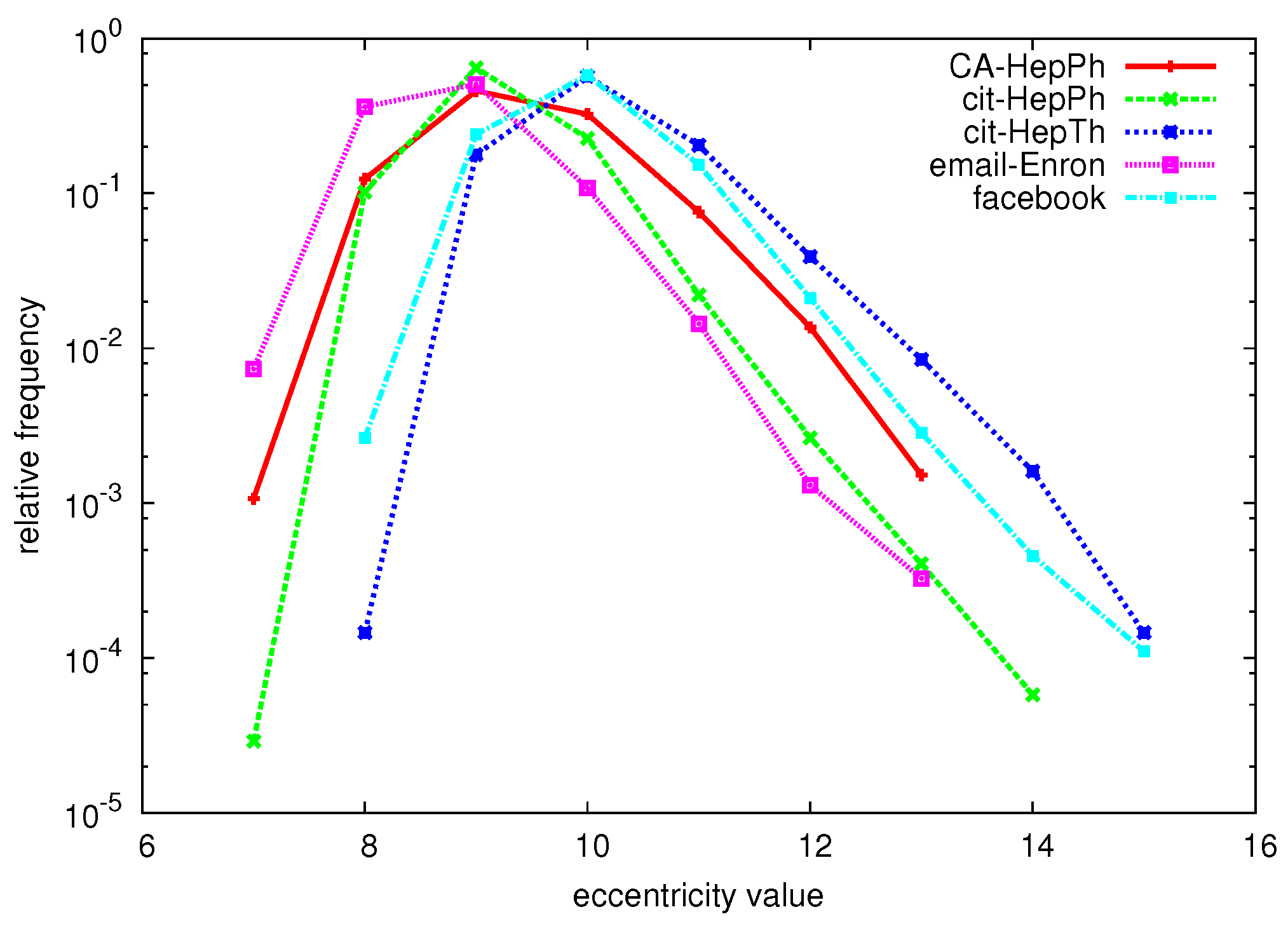
The eccentricity of a node is defined as the length of a longest shortest path from v to any other node: . The eccentricity distribution counts the frequency of each eccentricity value x, and can easily be derived when the eccentricity of each node in the graph is known. The relative eccentricity distribution lists for each eccentricity value x its relative frequency , normalizing for the number of nodes in the graph. Figure 1 shows the relative eccentricity distributions of a number of large graphs (for a detailed description of these datasets, see Section 6.1).
Figure 1.
Relative eccentricity distributions of various large graphs.

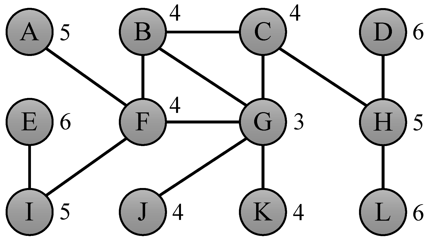
Various other measures can be derived using the notion of eccentricity, such as the average eccentricity of a graph G, defined as . Another related measure is the diameter of a graph G, which is is defined as the maximum eccentricity over all nodes in the graph: . Similarly, we define the radius of a graph G as the minimum eccentricity over all nodes in the graph: . The graph center refers to the set of nodes with an eccentricity equal to the radius, . Similarly, the graph periphery is defined as the set of nodes with an eccentricity value equal to the diameter of the graph: . Each of the measures explained above can be derived when the eccentricity of all nodes is known. Figure 2 shows an example of a graph that explains the different measures covered in this section.
Figure 2.
Toy graph showing the eccentricity of its 12 nodes, with average eccentricity 4.67, radius 3 realized by center node G, and diameter 6 realized by periphery nodes D, E and L.
Figure 2.
Toy graph showing the eccentricity of its 12 nodes, with average eccentricity 4.67, radius 3 realized by center node G, and diameter 6 realized by periphery nodes D, E and L.
Computing the eccentricity of one node can be done by running Dijkstra’s algorithm, and returning the largest distance found (i.e., the distance to a node furthest away from the starting node). Because we only consider unweighted graphs and thus, starting from the current node, can simply explore the neighboring nodes in level-order, computing the eccentricity of one node can be done in time. The process of determining the eccentricity of one node v is denoted by Eccentricities(v) in Algorithm 1.
| Algorithm 1 NaiveEccentricities |
1: Input: Graph G(V, E) 2: Output: Vector ε, containing ε(v) for all v ∈ V 3: for v ∈ V do 4: ε[v] ← ECCENTRICITY(v) // O(m) 5: end for 6: return ε |
This algorithm simply computes the eccentricity for each of the n nodes, resulting in an overall complexity of to determine the eccentricity of every node in the graph. Clearly, in graphs with millions of nodes and possibly hundreds of millions of edges, this approach is too time-consuming. The rest of this paper describes more efficient approaches for determining the eccentricity distribution, where we are interested in two things:
- The (relative) eccentricity distribution as a whole.
- Finding the extreme values of the eccentricity distribution, i.e., the radius and diameter, as well as derived measures such as the center and periphery of the graph.
We will address these issues by answering the following two questions:
3. Related Work
Substantial work on the eccentricity distribution dates back to 1975, when the term “eccentric sequence” was introduced to denote the sequence that counts the frequency of each eccentricity value [10]. The facility location problem is an example of the usefulness of eccentricity as a measure of centrality. When considering the placement of emergency facilities such as a hospital or fire station, assuming the map is modelled as a graph, the node with the lowest eccentricity value might be a good location for such a facility. In other situations, for example for the placement of a shopping center, a related measure called closeness centrality, defined as a node’s average distance to every other node (), is more suitable. Generally speaking, the eccentricity is a relevant measure when some strict criterion (the firetruck has to be able to reach every location within 10 minutes) has to be met [11]. An application of eccentricity as a measure on a larger scale is the network routing graph, where the eccentricity of a node says something about the worst-case response time between one machine and all other machines.
The most well-known eccentricity-based measure is the diameter, which has been extensively investigated in [5,6,7]. Several measures related to the eccentricity and diameter have also been considered. Kang et al. [12] study the effective radius, which they define as the 90th-percentile of all the shortest distances from a node. In a similar way, the effective diameter can be defined, which is shown to be decreasing over time for many large real-world graphs [13]. Each of these measures is computed by using an approximation algorithm [14] to determine the neighborhood of a node, a technique on which we will elaborate in Section 5.3.
To the best of our knowledge, there are no efficient techniques that have been specifically designed to determine the exact eccentricity distribution of a graph. Obviously, the naive approach, for example as suggested in [15], is too time-consuming. Efficient approaches for solving the APSP problem (which then makes determining the eccentricity distribution a trivial task) have been developed, for example using matrix multiplication [16]. Unfortunately, such approaches are still too complex in terms of time and memory requirements.
4. Exact Algorithm
In order to derive an algorithm that can compute the eccentricity of all n nodes in a graph faster than simply recomputing the eccentricity n times (once for each node in the graph), we have two options:
- Reduce the size of the graph as a whole to speed up one eccentricity computation.
- Reduce the number of eccentricity computations.
In this section we propose lower and upper bounds on the eccentricity, a strategy that accommodates the second type of speedup. We will also outline a pruning strategy that helps to reduce both the number of nodes that have to be investigated, as well as the size of the graph, realizing both of the two speedups listed above.
4.1. Eccentricity Bounds
We propose to use the following bounds on the eccentricity of all nodes , when the eccentricity of one node has been computed:
Observation 1 For nodes we have .
The upper bound can be understood as follows: if node w is at distance from node v, it can always employ v to get to every other node in steps. To get to node v, exactly steps are needed, totalling steps to get to any other node. The first part of the lower bound () can be derived in the same way, by interchanging v and w in the previous statement. The second part of the lower bound, itself, simply states that the eccentricity of w is at least equal to some found distance to w.
The bounds from Observation 1 were suggested in [6] as a way to determine which nodes could contribute to a graph’s diameter. We extend the method proposed in that paper by using these bounds to compute the full eccentricity distribution of the graph. The approach is outlined in Algorithm 2.
First, the candidate set W and the lower and upper eccentricity bounds are initialized (lines 3–8). In the main loop of the algorithm, a node v is repeatedly selected (line 10) from W, its eccentricity is determined (line 11), and finally all candidate nodes are updated (line 12–19) according to Observation 1. Note that the value of which is used in the updating process does not have to be computed, as it is already known because it was calculated for all w during the computation of the eccentricity of v. If the lower and upper eccentricity bounds for a node have become equal, then the eccentricity of that node has been derived and it is removed from W (lines 15–18). Algorithm 2 returns a vector containing the exact eccentricity value of each node. Counting the number of occurrences of each eccentricity value results in the eccentricity distribution.
An overview of possible selection strategies for the function SelectFrom can be found in [6]. In line with results presented in that work, we found that when determining the eccentricity distribution, interchanging the selection of a node with a small lower bound and a node with a large upper bound, breaking ties by taking a node with the highest degree, yielded by far the best results. As described in [6], examples of graphs in which this algorithm would definitely not work are complete graphs and circle-shaped graphs. However, most real-world graphs adhere to the small world property [17], and in these graphs the eccentricity distribution is sufficiently diverse so that the eccentricity lower and upper bounds can effectively be utilized.
| Algorithm 2 BoundingEccentricities |
1: Input: Graph G(V, E) 2: Output: Vector ε, containing ε(v) for all v ∈ V 3: W ← V 4: for w ∈ W do 5: ε[w] ← 0 εL[w] ← −∞ εU[w] ← +∞ 6: end for 7: while W ≠ Ø do 8: v ← SelectFrom(W) 9: ε[v] ← Eccentricities(v) 10: for w ∈ W do 11: εL[w] ← max(εL[w], max(ε[v] − d(v,w), d(v,w))) 12: εU[w] ← min(εU[w], ε[v] + d(v,w)) 13: if (εL[w] = εU[w]) then 14: ε[w] ← εL[w] 15: W ← W − {w} 16: end if 17: end for 18: end while 19: return ε |
Figure 3.
Eccentricity bounds of the toy graph in Figure 2 after subsequently computing the eccentricity of node G (left) and node E (right).
Figure 3.
Eccentricity bounds of the toy graph in Figure 2 after subsequently computing the eccentricity of node G (left) and node E (right).
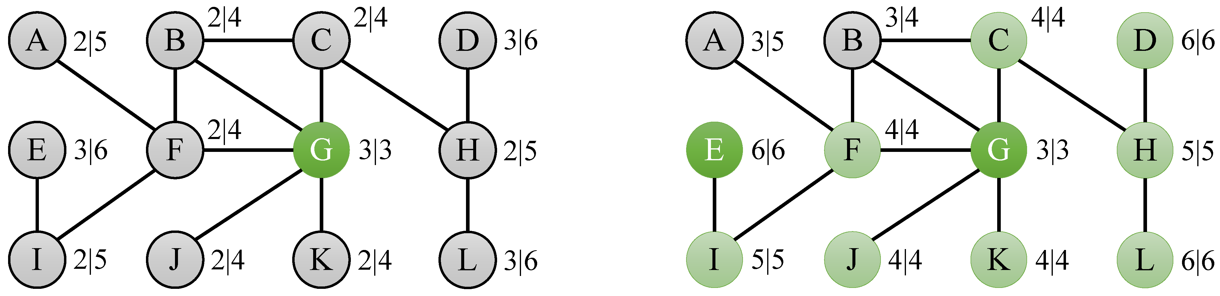
As an example of the usefulness of the bounds suggested in this section, consider the problem of determining the eccentricities of the nodes of the toy graph from Figure 2. If we compute the eccentricity of node G, which is 3, then we can derive bounds for the nodes at distance 1 (B, C, F, J and K), for the nodes at distance 2 (A, H and I) and for the nodes at distance 3 (D, E and L), as depicted by the left graph in Figure 3. If we then compute the eccentricity of node E, which is 6, we derive bounds for node I, for node F, for nodes A, B and G, for nodes C, J and K, for node K, and for nodes D and L. If we combine these bounds for each of the nodes, then we find that lower and upper bounds for a large number of nodes have become equal: for C, F, J and K, for H and I, and for D and L, as shown by the right graph in Figure 3. Finally, computing the eccentricity of nodes A and B results in a total of 4 real eccentricity calculations to compute the complete eccentricity distribution, which is a speedup of 3 compared to the naive algorithm, which would simply compute the eccentricity for all 12 nodes in the graph.
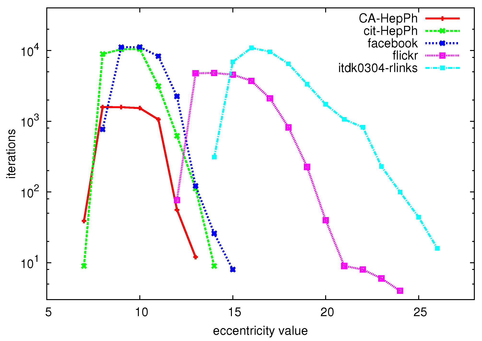
To give a first idea of the performance of the algorithm on large graphs, Figure 4 shows the number of iterations (vertical axis) that are needed to compute the eccentricity of all nodes with given eccentricity value (horizontal axis) for a number of large graphs (for a description of the datasets, see Section 6.1). We can clearly see that especially for the extreme values of the eccentricity distribution, very few iterations are needed to compute all of these eccentricity values, whereas many more iterations are needed to derive the values in between the extreme values.
Figure 4.
Eccentricity values (horizontal axis) vs. number of iterations to compute the eccentricity of all nodes with this eccentricity value (vertical axis).
Figure 4.
Eccentricity values (horizontal axis) vs. number of iterations to compute the eccentricity of all nodes with this eccentricity value (vertical axis).
4.2. Pruning
In this subsection we introduce a pruning strategy, which is based on the following observation:
Observation 2 Assume that . For a given , all nodes with have .
Node w is only connected to node v, and will thus need node v to reach every other node in the graph. If node v can do this in steps, then node w can do this is in exactly steps. The restriction on the graph size excludes the case in which the graph consists of v and w only.
All interesting real-world graphs have more than two nodes, making Observation 2 applicable in our algorithm, as suggested in [6]. For every node we can determine if v has neighbors w with . If so, we can prune all but one of these neighbors, as their eccentricity will be equal, because they all employ v to get to any other node. In Figure 2, node G has two neighbors with degree one, namely J and K. According to Observation 2, the eccentricity values of these two nodes are equal to JKG. The same argument holds for nodes D and L with respect to node H. We expect that Observation 2 can be applied quite often, as many of the graphs that are nowadays studied have a power law degree distribution [18], meaning that there are many nodes with a very low degree (such as a degree of 1).
Observation 2 can be beneficial to our algorithm in two ways. First, when computing the eccentricity of a single node, the pruned nodes can be ignored in the shortest path algorithm. Second, when the eccentricity of a node v has been computed (line 11 of Algorithm 2), and this node has adjacent nodes w with , then the eccentricity of these nodes w can be set to .
5. Sampling
Sampling is a technique in which a subset of the original dataset is evaluated in order to estimate (the distribution of) characteristics of the (elements in the) complete dataset, with faster computation as one of the main advantages. In this section we first discuss the use of sampling to determine the eccentricity distribution in Section 5.1. We focus on situations where we not only want to estimate the distribution of the eccentricity values, but also want to assess some parts of it (the extreme values) with higher reliability. For that purpose we propose a hybrid technique to determine the eccentricity distribution by that combines the exact approach from Section 4 with non-random sampling in Section 5.2. Finally in Section 5.3 we consider an adaptation of an existing approximation approach from literature.
5.1. Random Node Selection
If we want to apply sampling to the naive algorithm for obtaining the eccentricity distribution, we could choose to evaluate only a subset of size of the original n nodes, and multiply the values of the sampled eccentricity distribution by a factor to get an idea of the real eccentricity distribution, a process referred to as random node selection. Indeed, taking only a subset of the nodes would clearly speed up the computation of the eccentricity distribution and realize the second type of speedup discussed in Section 4. The trade-off here is that we no longer obtain the exact eccentricity distribution, but only get an approximation. The main question is then whether or not this approximation is representative of the original distribution. The effectiveness of sampling by random node selection with respect to various graph properties has been demonstrated in [19]. Using similar arguments as presented in [20,21], the absolute error can be assessed; indeed, when the chosen sampling subset is sufficiently large, the error is effectively bounded.
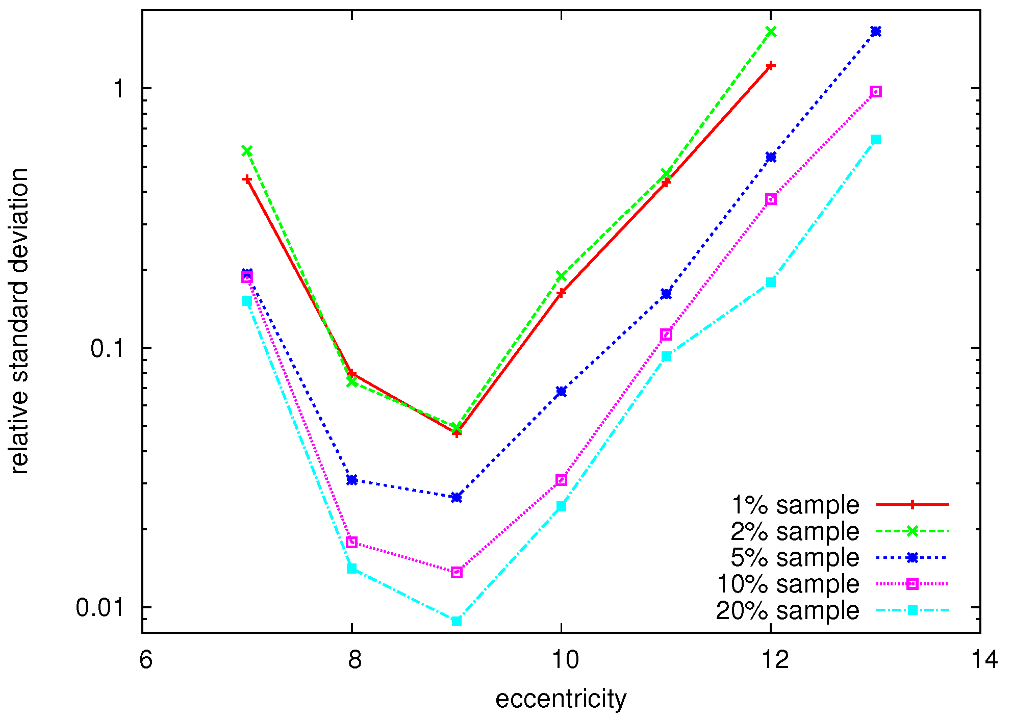
However, there are situations where we are not interested in minimizing the absolute error, but in minimizing the relative standard deviation (i.e., the absolute standard deviation divided by the mean) of the distribution of a particular eccentricity value. This especially makes sense when each eccentricity value is of equal importance, which might be the case when the extreme values of the distribution that are realizing the radius and diameter are of relevance. Let us consider an example. The real exact eccentricity distribution over all nodes in the ENRON dataset [22] is as follows:
| ε(v) | 7 | 8 | 9 | 10 | 11 | 12 | 13 |
| f(ε(v)) | 24 | 12 210 | 17 051 | 3 647 | 485 | 44 | 11 |
Figure 5 shows the relative standard deviation for each eccentricity value for different sample sizes (, , , , and ). For each sample size, we took 100 random samples to average the result. We note that low relative standard deviations can be observed for the more common eccentricity values (in this case, 8, 9 and 10). However, the standard deviation is quite large for the extreme values, meaning that on many occasions, the sample did not correctly reflect the frequency of that particular eccentricity value. Indeed, if only 11 out of 33,696 nodes () have a particular eccentricity value (in this case, a value of 13), we need a sample size of at least if we want to expect just one node with that particular eccentricity value. Even with a large sample size of , the standard deviation for the extreme value of 13 is very high (). For sample sizes of or , the eccentricity value of 13, that exists in the real distribution, was never even found. Similar events were observed for our other datasets, which is not surprising: the eccentricity distributions are tailed on the extremes, and these tails are likely to be left out in a sample. So clearly sampling does not suffice when extreme values of the eccentricity distribution have to be found, because such extreme values are simply too rare. However, for the more common eccentricity values, errors are very low, even for small sample sizes.
Figure 5.
Relative standard deviation (vertical axis) vs. eccentricity value (horizontal axis) for different random sample sizes of the Enron dataset.
Figure 5.
Relative standard deviation (vertical axis) vs. eccentricity value (horizontal axis) for different random sample sizes of the Enron dataset.

5.2. Hybrid Algorithm
From Figure 4,Figure 5 we can conclude that the exact approach is able to quickly derive the more extreme values of the eccentricity distribution, whereas a sampling technique is able to approximate the values in between the extremes with a very low error. Therefore we propose to combine the two approaches in order to quickly converge to an accurate estimation of the eccentricity distribution using a hybrid approach. This technique assumes that the eccentricity distribution has a somewhat unimodal shape, which is the case for all real-world graphs that we have investigated.
The sampling window consists of bounding variables ℓ and r that denote between which eccentricity values the algorithm is going to use the sampling technique. This window obviously depends on the distribution itself, which is not known until the exact algorithm has finished. Therefore we propose to set the value of ℓ and r dynamically, i.e., and . We furthermore change the stopping criterion in line 9 of Algorithm 2 to “while or do”. This means that the algorithm should stop when there are no more candidates that are potentially part of the center or the periphery of the graph. Note that these bounds apply to the candidate set W, but use information about all nodes V, ensuring that at least the center and periphery are known before the exact phase is terminated. When the exact algorithm has done its job, it can tighten ℓ and r even further, based on the eccentricity of the remaining candidate nodes: and . After this, ℓ and r become static, and the rest of the eccentricity distribution will be derived by using the sampling approach outlined in Algorithm 3. We will refer to the adjusted version of Algorithm 2 as BoundingEccentricitiesLR.
| Algorithm 3 HybridEccentricities |
1: Input: Graph G(V, E) and sampling rate q 2: Output: Vector f, containing the eccentricity distribution of G, initialized to 0 3: ε′ ← BoundingEccentricitiesLR(G, ℓ, r) 4: Z ← Ø 5: for v ∈ V do 6: if ε′[v] ≠ 0 and (ε′[v] ≤ ℓ or ε′[v] ≥ r) then 7: f[ε′[v]] ← f[ε′[v]] + 1 8: else 9: Z ← Z∪{v} 10: end if 11: end for 12: for i ← 1 to n·q do 13: v ← RandomFrom(Z) 14: ε[v] ← Eccentricities(v) 15: f[ε[v]] ← f[ε[v]] + (1/q) 16: Z ← Z − {v} 17: end for 19: return f |
Compared to Algorithm 2, the difference in terms of input is that the hybrid algorithm given in Algorithm 3 takes as input both the original graph and a sampling rate q between 0 and 1, where means that of the nodes have to be sampled. In Section 6 we will perform experiments to determine how q should be set. The result vector f holds the eccentricity distribution and is initialized based on the exact eccentricity values for values outside the sampling window (line 7). Nodes for which the exact eccentricity is not yet known are added to the candidate set Z (line 9). In lines 12–17, the eccentricity of a total of random nodes are calculated, and if this value lies within the specified window, the frequency of this eccentricity value is increased proportionally to the sample size. Finally, the eccentricity distribution f is returned.
5.3. Neighborhood Approximation
State of the art algorithms for computing the neighborhood function have been introduced in [12,14,23]. These algorithms can be adjusted as follows to also approximate the eccentricities. For an integer , the normalized size of the neighborhood of a node u can be defined as:
If we determine the value of for increasing values of h, then the eccentricity is the smallest h such that the approximated value of is sufficiently close to 1 or does not change in successive iterations.
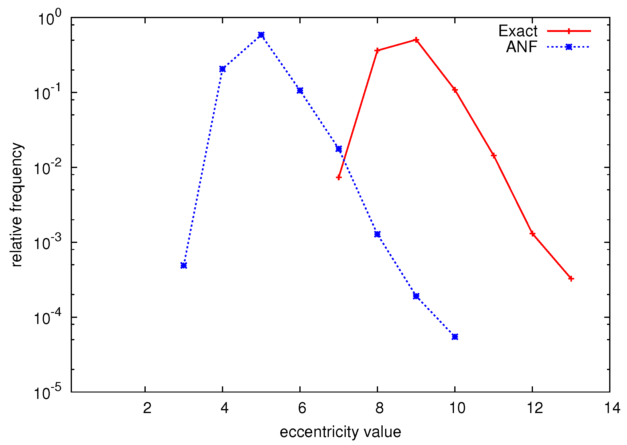
We have used the Approximate Neighborhood Function (ANF) [14] algorithm by Palmer et al. in order to approximate (by using the C source code available at the author’s website). Figure 6 shows the actual relative eccentricity distribution of the ENRON dataset, as well as the distribution that was approximated using the ANF-based approach. As ANF gives an approximate result, we averaged the result of 100 runs. We note that although the distribution shapes are very similar, ANF clearly underestimates the eccentricity values. We furthermore mention that the obtained distribution is clearly an approximation: a real eccentricity distribution would never have eccentricity values for which the smallest and largest value differ more than a factor of 2. Similar results were observed for other datasets, which leads us to believe that these approximation algorithms are not suitable for determining the eccentricity distribution, especially because they fail at assessing the extreme values of the distribution.
Figure 6.
Exact and approximated relative eccentricity distribution of the ENRON dataset.

6. Experiments
In this section we will use a number of large real-world datasets to assess the performance of both the exact algorithm from Section 4 and the hybrid algorithm from Section 5. The performance of our algorithms is measured by comparing the number of iterations and thus is independent of the hardware and software that were used for the implementation.
6.1. Datasets
We use a variety of network datasets, of which the name, type and source are listed in the first three columns of Table 1. The set of graphs covers a broad range of network types, including citation networks, collaboration networks, communication networks, peer-to-peer networks, protein-protein interaction networks, router topology networks, social networks and webgraphs. We will only consider the largest connected component of each graph, which is always the vast majority of the original graph. We also mention that some directed graphs have been interpreted as if they were undirected, and that self-edges and parallel edges are ignored. These factors may cause minor differences between the number of nodes and edges that we present here, and the numbers presented in the source papers. In Table 1 we also present for each dataset the exact average eccentricity , radius , diameter and center and periphery sizes and . For a more detailed description of these graphs, we refer the reader to the source papers in which the datasets were introduced.
Looking at the exact eccentricity distributions that we were able to compute, we can conclude that the distribution is not perfectly Gaussian as [32] suggests, but does appear to be unimodal. The distribution appears to be somewhat “tailed”; a positive skew is noticeable in Figure 1, which shows the relative eccentricity distribution of a number of graphs. The tail also becomes clear when comparing the average eccentricity value with the radius and diameter of the graph: for every dataset, the average eccentricity is closer to the radius. For example, for the CIT-HEPTH dataset with radius 8 and diameter 15, the average eccentricity is equal to .

Table 1.
Number of nodes, edges, average eccentricity, radius, diameter, center size and periphery size of our datasets.
| Dataset | Type | Source | Nodes | Edges | |||||
|---|---|---|---|---|---|---|---|---|---|
| YEAST | protein | [24] | 1 846 | 4 406 | 13.28 | 11 | 19 | 48 | 4 |
| CA-HEPTH | collab. | [25] | 8 638 | 49 612 | 12.53 | 10 | 18 | 74 | 4 |
| CA-HEPPH | collab. | [25] | 11 204 | 235 238 | 9.40 | 7 | 13 | 12 | 17 |
| DIP20090126 | protein | [26] | 19 928 | 82 406 | 22.01 | 15 | 30 | 1 | 2 |
| CA-CONDMAT | collab. | [13] | 21 363 | 182 572 | 10.58 | 8 | 15 | 6 | 11 |
| CIT-HEPTH | citation | [13] | 27 400 | 704 042 | 10.14 | 8 | 15 | 4 | 4 |
| ENRON | commun. | [22] | 33 696 | 361 622 | 8.77 | 7 | 13 | 248 | 11 |
| CIT-HEPPH | citation | [13] | 34 401 | 841 568 | 9.18 | 7 | 14 | 1 | 2 |
| SLASHDOT | commun. | [27] | 51 083 | 243 780 | 11.66 | 9 | 17 | 7 | 3 |
| P2P-GNUTELLA | peer-to-peer | [25] | 62 561 | 295 756 | 8.94 | 7 | 11 | 55 | 118 |
| social | [28] | 63 392 | 1 633 772 | 9.96 | 8 | 15 | 168 | 7 | |
| EPINIONS | social | [29] | 75 877 | 811 478 | 9.74 | 8 | 15 | 614 | 6 |
| SOC-SLASHDOT | social | [30] | 82 168 | 1 008 460 | 8.91 | 7 | 13 | 484 | 3 |
| ITDK0304-RLINKS | router | [26] | 190 914 | 1 215 220 | 17.09 | 14 | 26 | 155 | 7 |
| WEB-STANFORD | webgraph | [30] | 255 265 | 3 883 852 | 106.49 | 82 | 164 | 1 | 3 |
| WEB-NOTREDAME | webgraph | [31] | 325 729 | 2 180 216 | 27.76 | 23 | 46 | 12 | 172 |
| DBLP20080824 | collab. | [26] | 511 163 | 3 742 140 | 14.79 | 12 | 22 | 72 | 9 |
| EU-2005 | webgraph | [26] | 862 664 | 37 467 426 | 14.03 | 11 | 21 | 3 | 4 |
| FLICKR | social | [28] | 1 624 992 | 30 953 670 | 15.03 | 12 | 24 | 17 | 3 |
| AS-SKITTER | router | [13] | 1 694 616 | 22 188 418 | 21.22 | 16 | 31 | 5 | 2 |
6.2. Exact Algorithm
In order to determine the performance of the exact algorithm (Algorithm 2), we can count the number of shortest path computations that are needed to obtain the full distribution, and compare this value to n, the number of iterations performed by the naive algorithm (Algorithm 1). The number of iterations performed by our exact algorithm is displayed in the fourth column of Table 2, followed by the speedup factor compared to the naive algorithm. We note that significant speedups can be observed in terms of the number of iterations, especially for datasets for which the eccentricity distribution is wide, i.e., the difference between the radius and diameter is very large. We believe that this is due to the fact that the nodes that form the periphery of the network are sufficiently eccentric to have a large influence on the more central nodes, so that their lower and upper eccentricity bounds can very quickly be fixed by the bounding technique. We mention that the performance of our exact algorithm does not appear to be directly related to the number of nodes. The reduction in terms of the number of nodes as a result of our pruning strategy (see Section 4.2) is displayed in the column labeled “Pruned”, and is diverse, yet sometimes very significant (anywhere between and ).
To get a better idea of the performance of the algorithm, we propose to look at the quality of both the lower and upper bounds as the exact algorithm iterates over the candidate nodes. For this we define the measure of bound accuracy as the percentage of bound values that are correct at that iteration:
Here, is the actual eccentricity value, and is the (lower or upper) bound that we investigate. Figure 7 shows the lower and upper bound accuracy for a number of datasets. We can observe that for each of the datasets, after just a few iterations, the lower bound gives a very accurate indication of the actual eccentricity values. Apparently, the majority of the iterations are spent lowering the upper bound, whereas the lower bound quickly reflects the actual eccentricity distribution. Thus, in order to get an online estimate of the distribution, we could choose to consider only the lower bound, and obtain an accuracy of around 90% after only a handful of iterations.
Figure 7.
Bound accuracy vs. number of iterations for Algorithm 2.
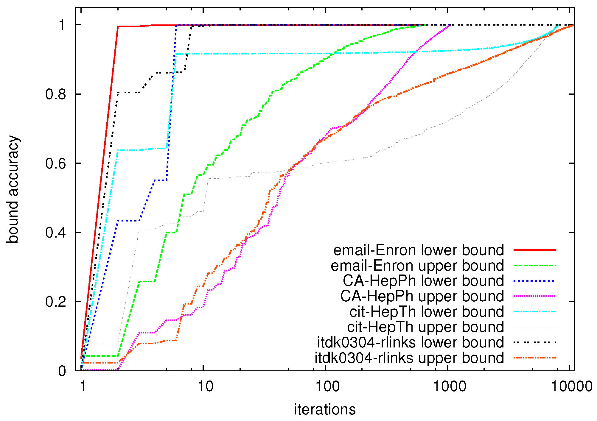
Table 2.
Performance (number of pruned nodes, number of iterations and speedup) of the exact algorithm (Algorithm 2) and the hybrid algorithm (Algorithm 3).
| Dataset | Nodes | Exact algorithm | Hybrid algorithm | |||||
|---|---|---|---|---|---|---|---|---|
| Pruned | Iterations | Speedup | Exact | Sampling | Total | Speedup | ||
| YEAST | 1 846 | 399 | 213 | 8.7 | 104 | 483 | 587 | 3.1 |
| CA-HEPTH | 8 638 | 351 | 1 055 | 8.2 | 150 | 350 | 500 | 17.3 |
| CA-HEPPH | 11 204 | 282 | 1 588 | 7.1 | 57 | 264 | 321 | 34.9 |
| DIP20090126 | 19 928 | 3 032 | 224 | 89.0 | 8 | 1321 | 1 329 | 15.0 |
| CA-CONDMAT | 21 363 | 353 | 3 339 | 6.4 | 73 | 388 | 461 | 46.3 |
| CIT-HEPTH | 27 400 | 140 | 8 104 | 3.4 | 57 | 444 | 501 | 54.7 |
| ENRON | 33 696 | 8 715 | 678 | 49.7 | 536 | 145 | 681 | 49.5 |
| CIT-HEPPH | 34 401 | 150 | 10 498 | 3.3 | 37 | 271 | 308 | 112 |
| SLASHDOT | 51 083 | 19,255 | 31 | 1648 | 24 | 180 | 204 | 250 |
| P2P-GNUTELLA | 62 561 | 16 413 | 21 109 | 3.0 | 8 575 | 177 | 8 752 | 7.1 |
| 63 392 | 1 075 | 11 185 | 5.7 | 780 | 168 | 948 | 66.9 | |
| EPINIONS | 75 877 | 20 779 | 4302 | 17.6 | 1 308 | 75 | 1 383 | 54.9 |
| SOC-SLASHDOT | 82 168 | 14 848 | 1460 | 56.3 | 990 | 156 | 1 146 | 71.7 |
| ITDK0304-RLINKS | 190 914 | 16 434 | 10 830 | 17.6 | 312 | 960 | 1 272 | 150 |
| WEB-STANFORD | 255 265 | 10 350 | 9 | 28 363 | 8 | 1 198 | 1 206 | 212 |
| WEB-NOTREDAME | 325 729 | 141,178 | 143 | 2277 | 94 | 1 381 | 1 475 | 4528 |
| DBLP20080824 | 511 163 | 22 579 | 42 273 | 12.1 | 150 | 355 | 505 | 1012 |
| EU-2005 | 862 664 | 26 507 | 59 751 | 14.4 | 71 | 1 630 | 1 701 | 507 |
| FLICKR | 1 624 992 | 553 242 | 4 810 | 338 | 200 | 1 618 | 1 818 | 932 |
| AS-SKITTER | 1 694 616 | 114 803 | 42 996 | 39.4 | 14 | 308 | 322 | 5502 |
6.3. Hybrid Algorithm
In our second set of experiments, we have evaluated the performance of the hybrid approach that incorporates sampling for the non-extreme values of the distribution (Algorithm 3). We will verify the quality of the obtained distribution by using the measure of distribution accuracy, defined as one minus the sum of the absolute difference between the eccentricity counts of real relative eccentricity distribution and the estimated distribution :
A distribution accuracy value of 1 indicates a perfect match between the actual and estimated relative eccentricity distributions. We note that for our hybrid approach, the error outside the sampling window is always equal to 0. As a result of the exact approach, we have access to the real eccentricity distribution. Therefore we can investigate the number of iterations that are needed to obtain an accuracy of in order to determine how we should set the sampling rate q. The sixth column of Table 2 shows the number of iterations needed to (exactly) compute the extreme values (center and periphery), which together with the column titled “Sampling” (averaged over 10 runs) results in the value denoted in column “Total”, which shows the total number of iterations needed to obtain an accuracy of . Apparently, for large graphs (over 100,000 nodes), a sampling rate of is more than sufficient to accurately derive the eccentricity distribution. An alternative would be to change the number of samples to a constant number, which would ensure that the number of eccentricity calculations does not exceed some fixed maximum.
An advantage of the exact approach is obviously that the nodes that have a certain eccentricity value can be pointed out exactly, whereas this is only possible for the extreme values in case of the hybrid approach. The hybrid approach does however improve upon the exact algorithm in terms of computation time (number of iterations) in many cases, especially for the larger graphs (over 100,000 nodes) with relatively tight eccentricity distributions, as can be seen in the rightmost column of Table 2. A bold value indicates the largest of the two speedups when comparing the hybrid approach and the exact approach. The exact approach performs better than the hybrid approach in a few cases, which we believe is due to the fact that the sampling phase should not have a too large window when the number of nodes is very small, because then a large number of iterations would be needed to obtain a representative sample of the distribution. This is especially the case for WEB-STANFORD, which has a very long tail. For this dataset, the exact algorithm performs really well, whereas the hybrid approach needs quite a few more iterations. We mention that, analogously to the performance of the exact algorithm, the performance of our hybrid algorithm does not appear to be correlated with the number of nodes.
From the experiments in this section we can generally conclude that we have developed a flexible approach for determining the eccentricity distribution of a large graph with high accuracy, while guaranteeing an exact result on the extreme values of the distribution (center and periphery of the graph).
7. Conclusions
In this paper we have studied means of computing the eccentricity of all nodes in a graph, resulting in the (relative) eccentricity distribution of the graph. It turns out that the eccentricity distribution of real-world graphs has an unimodal shape and tends to have a positive tail. We have shown how large speedups compared to the traditional method can be achieved by considering lower and upper bounds on the eccentricity, and by applying a pruning strategy. Even when the exact algorithm does not immediately give a satisfying result, the lower bounds proposed in this paper can serve as a reliable online estimate of the distribution as a whole.
We have also investigated the use of sampling as a means of computing the eccentricity distribution. The resulting hybrid algorithm uses the exact approach to derive the extreme values of the distribution and a sampling technique within a specific sampling window to accurately assess the values in between the extreme values. This results in an overall approach that is able to accurately determine the eccentricity distribution with only a fraction of the number of computations required by the naive approach.
In future work we would like to investigate the extent to which eccentricity and other centrality measures are related, and when the eccentricity can be used as a meaningful centrality measure. We are also interested in how the eccentricity distribution of a graph changes over time as the graph is evolving through the addition and deletion of nodes and edges.
Acknowledgments
We kindly thank the anonymous reviewers for providing useful and constructive comments on our paper. This research is part of the COMPASS project, financed by NWO under grant number 612.065.926.
References
- Sala, A.; Cao, L.; Wilson, C.; Zablit, R.; Zheng, H.; Zhao, B. Measurement-Calibrated Graph Models for Social Network Experiments. In Proceedings of the 19th ACM International Conference on the World Wide Web (WWW), Raleigh, NC, USA, 26–30 April 2010; pp. 861–870.
- Magoni, D.; Pansiot, J. Analysis of the autonomous system network topology. ACM SIGCOMM Comput. Commun. Rev. 2001, 31, 26–37. [Google Scholar] [CrossRef]
- Magoni, D.; Pansiot, J. Analysis and Comparison of Internet Topology Generators. In Proceedings of the 2nd International Conference on Networking Technologies, Services, and Protocols; Performance of Computer and Communication Networks; and Mobile and Wireless Communications, Pisa, Italy, 19–24 May 2002; pp. 364–375.
- Pavlopoulos, G.; Secrier, M.; Moschopoulos, C.; Soldatos, T.; Kossida, S.; Aerts, J.; Schneider, R.; Bagos, P. Using graph theory to analyze biological networks. BioData Min. 2011, 4, article 10. [Google Scholar] [CrossRef] [PubMed]
- Magnien, C.; Latapy, M.; Habib, M. Fast computation of empirically tight bounds for the diameter of massive graphs. J. Exp. Algorithm. 2009, 13, article 10. [Google Scholar] [CrossRef]
- Takes, F.W.; Kosters, W.A. Determining the Diameter of Small World Networks. In Proceedings of the 20th ACM International Conference on Information and Knowledge Management (CIKM), Glasgow, UK, 24–28 October 2011; pp. 1191–1196.
- Crescenzi, P.; Grossi, R.; Habib, M.; Lanzi, L.; Marino, A. On computing the diameter of real-world undirected graphs. Theor. Comput. Sci. 2012, in press. [Google Scholar] [CrossRef]
- Borgatti, S.P.; Everett, M.G. A graph-theoretic perspective on centrality. Soc. Netw. 2006, 28, 466–484. [Google Scholar] [CrossRef]
- Brandes, U. A faster algorithm for betweenness centrality. J. Math. Sociol. 2001, 25, 163–177. [Google Scholar] [CrossRef]
- Lesniak, L. Eccentric sequences in graphs. Period. Math. Hung. 1975, 6, 287–293. [Google Scholar] [CrossRef]
- Hage, P.; Harary, F. Eccentricity and centrality in networks. Soc. Netw. 1995, 17, 57–63. [Google Scholar] [CrossRef]
- Kang, U.; Tsourakakis, C.; Appel, A.; Faloutsos, C.; Leskovec, J. Hadi: Mining radii of large graphs. ACM Trans. Knowl. Discov. Data (TKDD) 2011, 5, article 8. [Google Scholar] [CrossRef]
- Leskovec, J.; Kleinberg, J.; Faloutsos, C. Graph evolution: Densification and shrinking diameters. ACM Trans. Knowl. Discov. Data (TKDD) 2007, 1, article 2. [Google Scholar] [CrossRef]
- Palmer, C.; Gibbons, P.; Faloutsos, C. ANF: A Fast and Scalable Tool for Data Mining in Massive Graphs. In Proceedings of the 8th ACM International Conference on Knowledge Discovery and Data Mining (KDD), Edmonton, Canada, 23–26 July 2002; pp. 81–90.
- Buckley, F.; Harary, F. Distance in Graphs; Addison-Wesley: Boston, MA, USA, 1990. [Google Scholar]
- Yuster, R.; Zwick, U. Answering Distance Queries in Directed Graphs Using Fast Matrix Multiplication. In Proceedings of the 46th IEEE Symposium on Foundations of Computer Science (FOCS), Pittsburgh, PA, USA, 23–25 October 2005; pp. 389–396.
- Kleinberg, J. The Small-World Phenomenon: An Algorithm Perspective. In Proceedings of the 32nd ACM symposium on Theory of Computing, Portland, OR, USA, 21–23 May 2000; pp. 163–170.
- Faloutsos, M.; Faloutsos, P.; Faloutsos, C. On power-law relationships of the internet topology. ACM SIGCOMM Comput. Commun. Rev. 1999, 29, 251–262. [Google Scholar] [CrossRef]
- Leskovec, J.; Faloutsos, C. Sampling from Large Graphs. In Proceedings of the 12th ACM International Conference on Knowledge Discovery and Data Mining (KDD), Philadelphia, PA, USA, 20–23 August 2006; pp. 631–636.
- Eppstein, D.; Wang, J. Fast Approximation of Centrality. In Proceedings of the 12th ACM-SIAM Symposium on Discrete Algorithms (SODA), Washington, DC, USA, 7–9 January 2001; pp. 228–229.
- Crescenzi, P.; Grossi, R.; Lanzi, L.; Marino, A. A Comparison of Three Algorithms for Approximating the Distance Distribution in Real-World Graphs. In Proceedings of the Theory and Practice of Algorithms in (Computer) Systems (TAPAS), LNCS 6595, Rome, Italy, 18–20 April 2011; pp. 92–103.
- Klimt, B.; Yang, Y. The Enron Corpus: A New Dataset for Email Classification Research. In Proceedings of the 15th European Conference on Machine Learning (ECML), LNCS 3201, Pisa, Italy, 20–24 September 2004; pp. 217–226.
- Boldi, P.; Rosa, M.; Vigna, S. HyperANF: Approximating the Neighbourhood Function of very Large Graphs on a Budget. In Proceedings of the 20th ACM International Conference on the World Wide Web (WWW), Hyderabad, India, 16–20 April 2011; pp. 625–634.
- Jeong, H.; Mason, S.; Barabási, A.; Oltvai, Z. Lethality and centrality in protein networks. Nature 2001, 411, 41–42. [Google Scholar] [CrossRef] [PubMed]
- Leskovec, J.; Kleinberg, J.; Faloutsos, C. Graph evolution: Densification and shrinking diameters. ACM Trans. Knowl. Discov. Data 2007, 1, article 2. [Google Scholar] [CrossRef]
- Sommer, C. Graphs. Available online: http://www.sommer.jp/graphs (accessed on 1 September 2012).
- Gómez, V.; Kaltenbrunner, A.; López, V. Statistical Analysis of the Social Network and Discussion Threads in Slashdot. In Proceedings of the 17th International Conference on the World Wide Web (WWW), Beijng, China, 21–25 April 2008; pp. 645–654.
- Mislove, A.; Marcon, M.; Gummadi, K.; Druschel, P.; Bhattacharjee, B. Measurement and Analysis of Online Social Networks. In Proceedings of the 7th ACM Conference on Internet Measurement, San Diego, CA, USA, 24–26 October 2007; pp. 29–42.
- Richardson, M.; Agrawal, R.; Domingos, P. Trust Management for the Semantic Web. In Proceedings of the 2nd International Semantic Web Conference (ISWC), LNCS 2870, Sanibel Island, FL, USA, 20–23 October 2003; pp. 351–368.
- Leskovec, J.; Lang, K.; Dasgupta, A.; Mahoney, M. Community structure in large networks: Natural cluster sizes and the absence of large well-defined clusters. Int. Math. 2009, 6, 29–123. [Google Scholar] [CrossRef]
- Barabási, A.; Albert, R.; Jeong, H. Scale-free characteristics of random networks: The topology of the world-wide web. Phys. Stat. Mech. Appl. 2000, 281, 69–77. [Google Scholar] [CrossRef]
- Magoni, D.; Pansiot, J. Internet Topology Modeler Based on Map Sampling. In Proceedings of the 7th International Symposium on Computers and Communications (ISCC), Taormina, Italy, 1–4 July 2002; pp. 1021–1027.
© 2013 by the authors; licensee MDPI, Basel, Switzerland. This article is an open access article distributed under the terms and conditions of the Creative Commons Attribution license (http://creativecommons.org/licenses/by/3.0/).
Share and Cite
MDPI and ACS Style
Takes, F.W.; Kosters, W.A. Computing the Eccentricity Distribution of Large Graphs. Algorithms 2013, 6, 100-118. https://doi.org/10.3390/a6010100
AMA Style
Takes FW, Kosters WA. Computing the Eccentricity Distribution of Large Graphs. Algorithms. 2013; 6(1):100-118. https://doi.org/10.3390/a6010100
Chicago/Turabian StyleTakes, Frank W., and Walter A. Kosters. 2013. "Computing the Eccentricity Distribution of Large Graphs" Algorithms 6, no. 1: 100-118. https://doi.org/10.3390/a6010100