
Carbon Dioxide Fluxes and Their Environmental Controls in a Riparian Forest within the Hyper-Arid Region of Northwest China


1
Northwest Institute of Eco-Environment and Resources, CAS, Lanzhou 730000, China
2
Key Laboratory of Eco-hydrology of Inland River Basin, CAS, Lanzhou 730000, China
3
University of Chinese Academy of Sciences, Beijing 100049, China
4
School of Agricultural, Computational and Environmental Sciences, Institute of Agriculture and Environment (I Ag&E), University of Southern Queensland, Springfield, Queensland 4300, Australia
*
Author to whom correspondence should be addressed.
Forests 2017, 8(10), 379; https://doi.org/10.3390/f8100379
Submission received: 3 July 2017
/
Revised: 27 September 2017
/
Accepted: 28 September 2017
/
Published: 4 October 2017
(This article belongs to the Section Forest Ecology and Management)
Abstract
:Hyper-arid regions are expected to undergo climatic change, but only a few research works have so far been conducted on the dynamics of carbon dioxide (CO2) fluxes and their consequent responses to various bioclimatic factors, which is mainly attributable to a limited set of flux observations. In this study, the CO2 fluxes exchanged between the forest and the atmosphere have been measured continuously by the eddy covariance approach from June 2013 to December 2016 in a riparian forest, which is a primary body of natural oases located within the lower reaches of inland rivers in China. The present results revealed that the climatic conditions characterized by relatively high mean air temperatures (Ta) with fluctuating annual precipitation (P) during the prescribed study periods were comparable to the historical mean value. The annual net ecosystem productivity (NEP) ranged from approximately 278 g C m−2 year−1 to 427 g C m−2 year−1, with a mean value of 334 g C m−2 year−1. The mean annual ecosystem respiration (Re) and the gross primary productivity (GPP) were found to be 558 and 892 g C m−2 year−1, respectively. The results also ascertained that the high inter-annual variations in NEP were attributable to Re rather than to GPP, and this result was driven primarily by Ta and the groundwater depth under similar eco-physiological processes. In addition, the CO2 fluxes were also strongly correlated with the soil temperature and photosynthetically active radiation for the present study site. In conclusion, the desert riparian forest is a considerably significant carbon sink, particularly in the hyper-arid regions.
1. Introduction
Terrestrial ecosystems have been acting as a substantial sink for atmospheric carbon dioxide (CO2), which is evidenced by approximately 2.6 ± 0.8 PgC year−1 of CO2 that have been sequestrated in the last decade (i.e., 2002–2011) [1]. However, climate change projections show that there could be a large uncertainty in terms of the magnitude and the sign of terrestrial carbon storage, which could be associated with the differences in the global and regional models [2,3]. For terrestrial ecosystems, although the mean carbon sink is dominated by highly productive lands (mainly comprised of tropical forests), the trends and inter-annual variability of the carbon sinks are dominated by semi-arid ecosystems whose carbon balance is strongly associated with the circulation-driven variations in both the air/land surface temperatures and precipitation [4,5]. However, we have a limited knowledge on the carbon source/sink intensity and its respective variability in arid ecosystems. In particular, due to the scarcity of precipitation, the groundwater is the main source required to maintain the current structure and functions in hyper-arid regions [6,7,8]. In addition, these ecosystems are highly vulnerable to climate change, e.g., invasive species success [9], therefore an understanding of the extent of carbon sequestration and emissions including the underlying driving forces behind this process is crucial for estimating the overall carbon balance in arid ecosystems. Such knowledge is also likely to contribute to the prediction of carbon balance based on different types of future climate change scenarios.
In addition to the traditional forest inventory-based approaches [10], the eddy covariance method has been widely used to estimate the carbon balance of forest ecosystems [11], in which the net ecosystem exchange of CO2 (NEE) between the vegetation and the atmosphere can thus be measured directly and continuously in the long-term period [12]. Many of those studies have concentrated on the carbon storage variations [11,13], mechanisms [14], disturbances [15,16] and the capacity of forest environments to foster carbon sequestration [10,17], however, most of these studies have been conducted in tropical, temperate and boreal forest environments [10,15,18]. In spite of the hyper-arid regions being expected to undergo climatic change [4,19], only a few research works have so far been conducted on the dynamics of carbon dioxide fluxes and their responses to bioclimatic factors, due to the presence of the limited carbon flux datasets, especially in water-limited ecosystems [20,21]. For example, the study of Zhou et al. [21] has examined seasonal and inter-annual variability of carbon dioxide fluxes and their responses to drought events in a poplar plantation in Northern China. Garcia-Franco et al. [22] investigated the carbon dynamics after an afforestation of semiarid shrub lands, and showed that the carbon sequestration can be increased by applying the suitable afforestation techniques. The study of Smith et al. (2000) demonstrated that the elevated levels of CO2 are likely to increase forest production in the arid region of the southwestern USA [9]. These studies have shown that the forest ecosystems in arid regions are reasonable potential carbon pools and are sensitive to the changes in environmental conditions. However, little attention has been paid to the riparian forests that are dependent on the groundwater in hyper-arid regions, although the riparian cottonwood (Populus fremontii S. Watson) forest in northern California’s Central Valley (310 g C m−2 year−1) [23] and the riparian mesquite woodland along the San Pedro River in southeastern Arizona (233 g C m−2 year−1) [24], USA remain an exception.
Riparian forests represent a primary body of natural oases in the lower reaches of inland rivers in China [25]. For example, the Ejin oasis, which is surrounded by a wide desert and located in the lower Heihe River Basin (HRB), exhibits harsh natural conditions with a dry climate, and the ecosystems in this region are highly vulnerable to climate change [26]. In this hyper-arid region, the Ejin oasis on river sides represents some of the richest desert ecosystems, populated with riparian forest, which is internally controlled and interacts with surrounding deserts [27]. Although the area of the riparian forest in Ejin is not large, there are lot of species of biological importance, and their growth and succession reflect the overall health and stability of the Ejin Oasis [28]. Moreover, the desert riparian forest maintains energy and matter cycles in desert regions [7]. The study of CO2 fluxes and their environmental controls may provide insights into the health and activities of the riparian forest. Survival, growth and development of riparian forests have largely been dependent on the groundwater [6,8]. The overexploitation of water resources in the middle reaches of HRB since the 1960s led to a decrease in the discharge of water to its lower reaches, that was also likely contributing to a consequent decline in the groundwater and a degradation of ecosystems along the riparian habitats [29]. To restore the deteriorated eco-hydrological environment in the lower HRB region, the ecological water conveyance project (EWCP) was established in the year 2000, and the water resources have thus undergone strict artificial controls. As a result of the implementation of this artificial water management system, groundwater levels appear to have increased, and the vegetation has experienced a favorable change [30]. Groundwater, as the only available water source, has been used to meet the demands for domestic water supply and the ecologic-environmental water consumption. Therefore, it is essential to investigate the dynamics of carbon storage under artificial water management in this important region.
Considering the need for examining the characteristics of CO2 fluxes and their environmental controls in a riparian forest within the hyper-arid region of Northwest China, the continuous measurements in CO2 fluxes were carried out using the eddy covariance technique. The purpose of this study was to analyze the capacity, variability and the major environmental controlling factors of carbon dioxide fluxes in the desert riparian forest. This study is expected to broaden our understanding of the response processes and the mechanisms in place for the carbon balance of riparian forests in arid regions to face the further climate change and human activities such as artificial water management controls.
2. Materials and Methods
2.1. Site Description
The present study area is located at the lower reach of HRB region, northwest China. The climate in this region is hyper-arid [31], with the mean annual precipitation (P) being approximately 37.5 mm and the pan evaporation (Ep) being approximately 2240.5 mm according to data collected for the period 1957–2016 from the Ejin Meteorological station provided by China Meteorological Data Sharing Services. The aridity index is less than 0.05 in this region. Mean annual temperature is estimated to be 8.9 °C, with a mean monthly temperature ranging from −11.5 °C in January to 27.0 °C in July. The P shows an obvious seasonal pattern (with approximately 75% of the rainfall falling during June–October period) with significant inter-annual variations (of approximately 7–103 mm for the present study period 1957–2016) (Table S1).
The observation stand is situated at the Qidaoqiao P. euphratica Forest National Natural Refuge (Figure 1, 41°59′ N, 101°10′ E, 920.46 m elevation) [31,32]. The study site contains one of the best-grown riparian forests in the lower HRB region. The riparian forest in the study area is composed of Populus euphratica Oliv. (P. euphratica) and Tamarix ramosissima Ledeb. (T. ramosissima) [32]. The P. euphratica is the dominant plant species with a density of 320 stems ha−1, and contributes approximately 75% of the total basal area in the study region [32]. The characteristics of P. euphratica including tree height (10.1 ± 1.7 m), canopy height (5 m), diameter at breast height (DHB, 22.9 ± 4.8 cm), mean age (40 years) and canopy coverage (52%) were measured in a 100 m × 100 m plot. Moreover, the soils in the P. euphratica stand consist of a sandy loam approximately 2 m deep and which has a saturated volumetric water content of 0.35 m3 m−3 [31]. At the study site, the mean groundwater depth (GWD) was 1.4 m. In order to acquire the data, the eddy covariance instruments were installed at a relatively flat and homogenous ground, and the dominant plants extended for several kilometers in all directions. The site’s roughness length, zero-displacement height and slope were 1.38 m, 7.9 m and 1/5000, respectively. The prevailing wind was from southeast and northwest directions and the measured fluxes originated between 109 and 1520 m from the tower (i.e., peak at 228 m) in the prevailing wind direction. The peak of about 228 m represented the area with the highest carbon dioxide flux contribution in the footprint.
2.2. Eddy Covariance and Meteorological Measurements
Carbon dioxide fluxes were measured from June 2013 to December 2016, using the eddy covariance method. A 22-m-tall steel scaffold flux tower was established in the forest where the terrain was relatively flat with a highly homogenous land cover surface. The instruments included a three-dimensional sonic anemometer (CSAT3, Campbell Scientific, Inc., Logan, UT, USA) used to measure 3 coordinate speeds (u, v, w), and an open-path CO2/H2O infrared gas analyzer (LI-7500, LI-COR Inc., Lincoln, NE, USA) used to measure the water vapor density and carbon dioxide fluctuations, installed at 20 m above the ground. Air temperature (Ta, °C) and relative humidity (RH, %) were also measured at 20 m above the ground surface by air temperature/relative humidity sensors (HMP45C, Campbell Scientific, Logan, UT, USA). The turbulence fluxes and Ta and RH data were recorded by a CR3000 data logger (Campbell) at a 10 Hz sampling frequency, and the 30 min averages were computed.
In addition, the solar radiation components (i.e., upward and downward shortwave radiation and longwave radiation) were measured at 10 m above the ground by a 4-Component Net Radiation Sensor (CNR4, Kipp & Zonen, Delft, The Netherlands), and the net radiation (Rn, W m−2) was calculated as the difference of the net shortwave radiation and the net longwave radiation. One quantum sensor (LI-190SA, Li-COR Inc.) was mounted at an approximately 6 m height above the ground to measure the photosynthetically active radiation (PAR, μ mol·m−2·s−1). Two soil heat flux plates were buried at approximately 5 cm below the soil surface to measure the soil heat flux (G, W m−2). These data were recorded by a CR1000 data logger (Campbell).
2.3. Eddy Covariance Flux Calculations and Data Quality Control
The half-hour NEE (net ecosystem exchange of CO2) amounts were calculated by Eddypro software (LI-COR Inc.) following standard quality control procedures, including despiking, 2D coordinate rotation, time lag removal, frequency response correction using model spectra and transfer functions [33] and air density correction [34]. Additional outliers still existed under the procedure as stated below, thus they needed to be screened and then removed through several steps using the data quality assurance and control (QA/QC) procedures:
- (1)
- According to the empirical values of the CO2 fluxes and the statistical analyses of data, the scope of the threshold was defined, which ranged from approximately −60 to 60 μ mol m−2 s−1. All data outside of the threshold were removed;
- (2)
- Because of the complex structures, the eddy covariance instruments are susceptible to instability generated within the circuits, from dust and moisture in the air, precipitation, human operation, etc. Therefore, the spikes in the data appeared occasionally. For this reason, these spikes were filtered using the analysis of variance test [35] and 4 standard deviations were selected;
- (3)
- Because “photosynthesis” is unlikely to occur during the night, the occasional negative CO2 fluxes during the night were also filtered; and
- (4)
- A friction velocity (u*) threshold was used to filter the fluxes at night when the atmospheric turbulence was not well developed. The threshold for u* was estimated by the Moving Point Test as described in literature [36]. The flux data were discarded when the corresponding u* value was less than the threshold value.
2.4. Data Gaps Filling and NEE Partitioning
The filtered NEE and meteorological data gaps were filled with appropriate methods considering the co-variation of the fluxes with meteorological variables and the temporal auto-correlation of the fluxes [37], according to the online procedure (https://www.bgcjena.mpg.de/bgi/index.php/Services/REddyProcWebMethod). Following this, the mean diurnal method (MDM) was applied to fill residual gaps found in the dataset.
Since only the NEE can be measured directly by the eddy covariance method, it was partitioned using the same online procedure to gain gross primary production (GPP) and ecosystem respiration (Re), in accordance with Equation (1) [37]. First, an activation energy parameter (E0) was estimated for the yearly dataset. Next, the reference temperature (Rref) was estimated with a seven-day sliding window in steps of four days. If Rref was not found in some sub-periods, its value was linearly interpolated. Third, the NEE was partitioned into GPP and Re using the estimated values of E0 and Rref. Only the nighttime original data after QA/QC were used in the estimation of E0, and the other datasets (i.e., the gap-filled data) were used in the partitioning of NEE:
where the Rref was the respiration rate at reference temperature (Tref, 15 °C), E0 was a free parameter, which essentially determined the temperature sensitivity and T0 was kept constant at −46.02 °C [37]. To compare the magnitude of carbon dioxide flux components, the NEE was represented by net ecosystem production (NEP = −NEE), and together with GPP and Re were given as positive values at monthly and yearly time-scales, and which were also used to determine the relationship with meteorological factors at different time-scales.
2.5. Groundwater Depth and Soil Moisture and Salt Measurement
Within the present study site, a well located at a distance of 30 m away from the EC tower and 100 m from one tributary was drilled to about 6 m depth; while an automatic pressure transducer (HOBO-U20, Onset Computer Corporation, Bourne, MA, USA) was installed in order to monitor the changes in the submerged pressure (Psub, kPa) at 0.5 h intervals. The recorded atmospheric pressure (Pa, kPa) from the EC tower was subtracted from Psub in order to obtain the pressure that was exerted only by the water column above the sensors. Water head data were then converted to the groundwater depth (GWD, m), using the measured distance between sensors and the ground surface at the observation well. The ground water depth (GWD) refers to the distance from the underground water to the surface, and the values can be positive according to other researchers [38]. The larger the value is, the deeper the groundwater is.
In 2015 and 2016, the soil moisture/salts/temperature sensors (SMEC 300, Spectrum Technologies, Inc., Aurora, IL, USA) were installed at 10, 30, 50 and 80 cm depths in six positions (i.e., in two directions, north and west, and three distances of 50, 150 cm and 250 cm from the selected trees) in order to obtain the soil volumetric moisture content (θ, %) and the electrical conductivity (EC, mS cm−1). These were used to reflect the soil moisture and salt regime in the stand, respectively. The mean values of the different directions and distances were used to analyze the temporal variations in θ and EC of the stand.
2.6. Data Analysis
The daytime and nighttime periods were separated according to the global radiation threshold of 20 W m−2 [37]. The half-hour CO2 fluxes were integrated to their respective daily, monthly and annual periods using Microsoft Excel 2007 Software and MATLAB software. For the meteorological factors, the monthly mean values of Ta, RH, Ep and GWD, and the mean annual Ta and total annual P, were calculated in the period 2013–2016 and as historical averages (1957–2016). The meteorological data were recorded by the Ejin weather station and provided by China Meteorological Data Sharing Services. Daily mean soil temperature (Ts), VPD, PAR and GWD were also used to determine the major controlling factors of the carbon fluxes, i.e., NEE, GPP and Re, using appropriate correlation analysis. The Spearman correlations were calculated by SPSS Statistics software package V.16 (SPSS Inc., Chicago, IL, USA).
3. Results
3.1. Weather Conditions
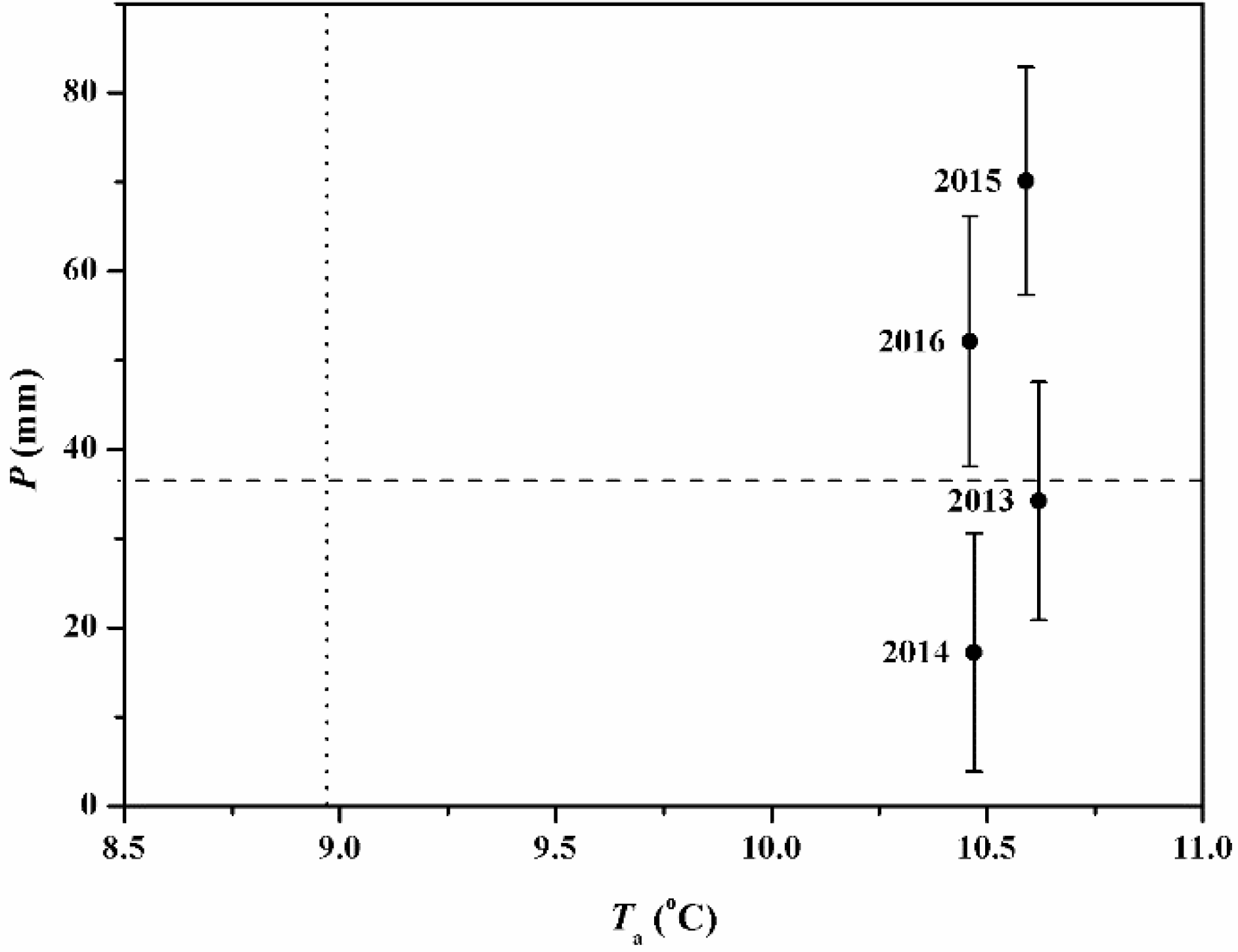
The differences between average Ta and P for the period 2013–2016 and the historical averages have been analyzed in Figure 2. The climatic conditions during the study period were characterized by the high average Ta, with the fluctuant annual P component (Figure 2). Annual mean Ta values for the period 2013–2016 were all above the mean annual level (1957–2016) whereas the annual P levels were near the historical average (37.5 mm) in 2013 (34.2 mm), above the historical average in 2015 (70.1 mm) and 2016 (52.1 mm) and below the historical average in 2014 (17.2 mm).
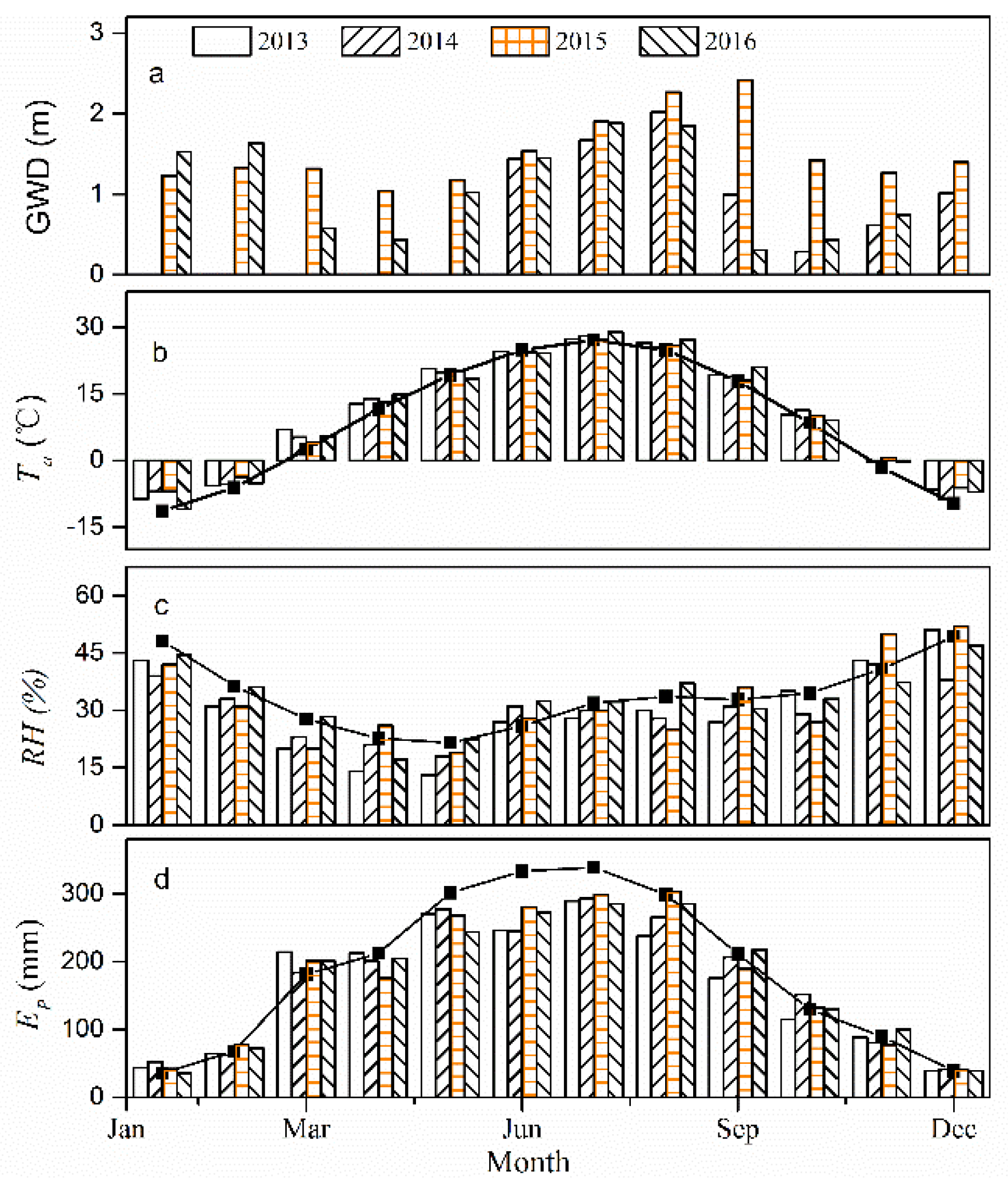
In this study, we have also characterized the climatic conditions for the period 2013–2016 and thus analyzed the discrepancies between the respective study-year values with the historical means representing the environmental factors (Figure 3). The annual mean Ta values were 10.62, 10.47, 10.59 and 10.46 in 2013–2016, respectively. Moreover, the mean values of Ta during these four growing seasons were 21.45, 21.30, 20.98 and 21.46 °C, respectively (Table 1). The average GWD in the stand was 1.4 m for 2014–2016 and the variations in GWD mainly depended on the amount and the time of the water conveyance activities. Generally, the arrival time of water allocations was concentrated around the months of September and October and the values of GWD decreased rapidly following the entry of water and then increased gradually until the next water allocation.
Mean monthly GWD values for the period May to October 2015 were found to be greater than those in 2014 and 2016. The mean monthly RH values ranged between 13% and 52% for the period 2013–2016, with a relatively lower value in April and May. In terms of RH, the values were similar from July to October ranging from 27% to 37%. In addition, the annual Ep registered the values of 1997, 2062, 2090 and 2087 mm, respectively, while the monthly maximum for each year was found to be about 289.4 mm (July), 293.2 mm (July), 303.9 mm (August) and 285.4 mm (July) in 2013–2016, respectively. Compared to historical mean values, the monthly Ep values were lower in the period of May-October, owing to the lower wind speed values as described in other studies (e.g., [39]), except for the month of October 2014.
In contrast to the meteorological variables measured in this paper, the soil hydrological regime was greatly affected by the flood irrigation, as revealed in Figure 4. Daily θ values registered similar patterns to the GWD data, exhibiting a decrease with an increase in GWD over the passage of time during the growing season, which in fact, showed a sudden increase after the flood irrigation. In the vertical profile, the values of θ exhibited an increase with increasing depths (Figure 4a), while the electrical conductivity (EC, mS cm−1) varied in agreement with θ data, which also appeared to be disturbed by flood events. However, the highest values of EC were observed at the 50 cm depths for most of the measurement period, as shown in Figure 4b. The mean value of EC acquired at different depths for the 2015 period (i.e., 0.46 mS cm−1) was significantly lower than those for the 2016 period (i.e., 0.86 mS cm−1; p < 0.001).
3.2. Multi-Scale Temporal Variations of Carbon Fluxes
3.2.1. Daily Time Scale
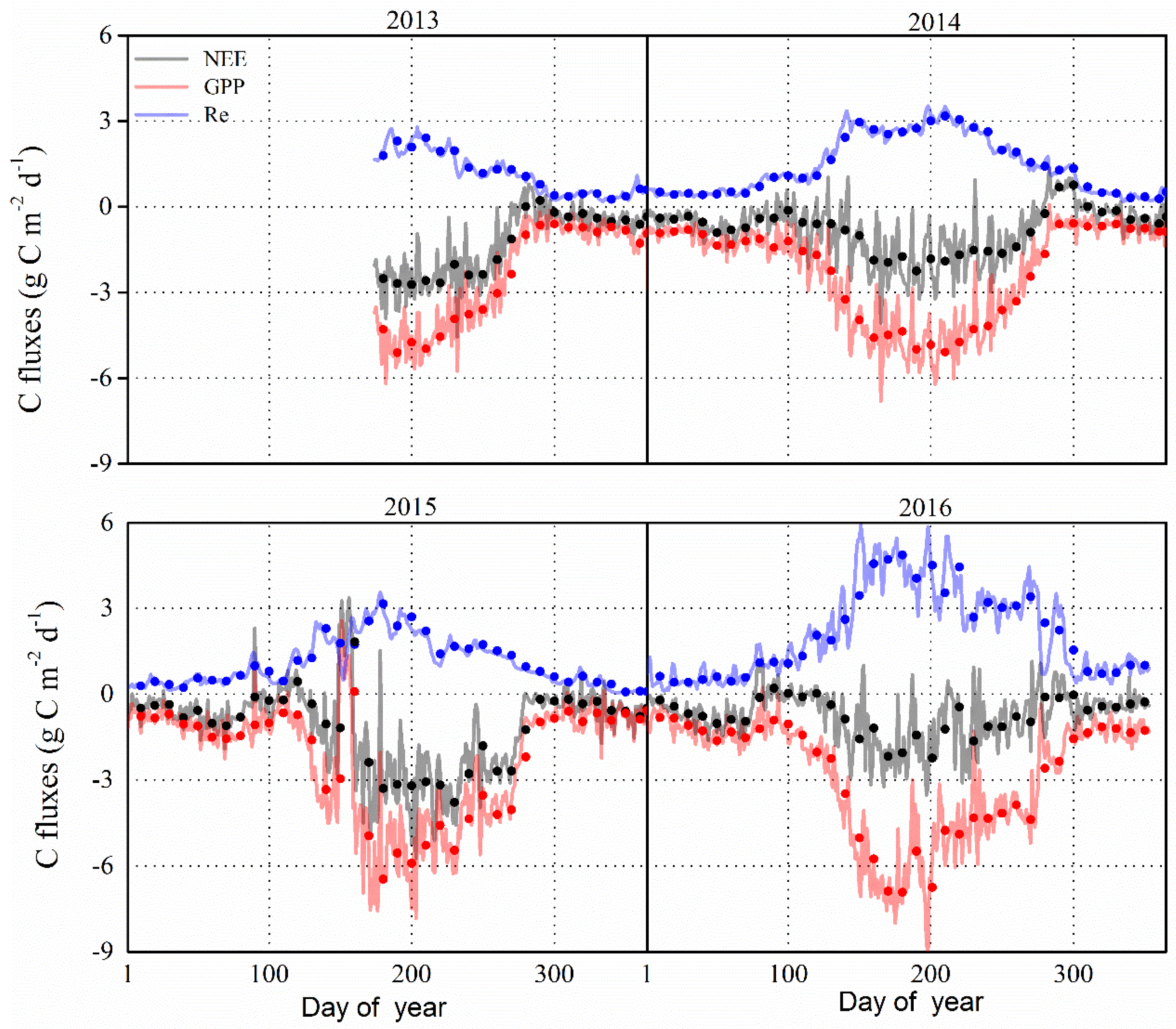
The inter-annual and seasonal variations in daily carbon dioxide fluxes (i.e., NEE, GPP, Re) in the P. euphratica stand are shown in Figure 5. In this figure, the seasonal pattern of GPP was found to exhibit a similar pattern for the period 2013–2016. The NEE appeared to increase rapidly with the sprout of trees since early May, and then, it fluctuated following the variation in temperature and the available water resources during the months from June to August, and declined after the onset of the leaf senescence period (i.e., September). There is no obvious variation in CO2 fluxes during the non-growing season. In addition, the GPP and Re showed the same tendency of variation for the period 2013–2016. The daily mean NEE ranged from −4.55 to 0.79, −4.07 to 1.35, −5.74 to 3.36 and −3.52 to 1.14 g C m−2 d−1 g C m−2 d−1 during the growing season in 2013–2016, respectively.
The daily maximum GPP values were found to be −5.97 (1 July), −6.81 (14 June), −7.82 (26 June) and −9.08 (16 July) g C m−2 d−1 in 2013–2016, respectively, while the daily Re showed seasonal peaks of 2.78 (23 July), 3.52 (17 July), 3.68 (27 June) and 5.85 (16 July) g C m−2 d−1 in 2013–2016, respectively. Accordingly, the maximum NEE were found to be relatively higher in 2015 than the other three years. In fact, higher Re values were found in 2016 compared to other three years, and coincided with higher values of GPP. The mean values of maximum NEE, GPP and Re in 2013–2016 were −4.47, −7.42 and 3.96 g C m−2 day−1, respectively. On the other hand, the length of the C uptake period was similar during the growing season across the four years, and the number of C sink days were approximately 153, 167 and 158 days for the period 2014–2016, respectively.
3.2.2. Monthly Time Scale
The monthly carbon balance components (i.e., NEP, GPP, and Re) were varied among the four years (Figure 6). During the growing season of 2013–2016, the monthly mean NEP value was 43.91 g C m−2 month−1, with the maximum of 70.52 g C m−2 month−1 in July and a minimum of 1.27 g C m−2 month−1 in October. In October, the forests acted as a carbon source in 2014 (NEP was equal to −13.17 g C m−2 month−1), and as a carbon sink in 2015 (i.e., NEP was equal to 11.38 g C m−2 month−1) and in 2016 (i.e., NEP was equal to 6.21 g C m−2 month−1), and remained a neutral in 2013 (i.e., NEP was equal to 0.67 g C m−2 month−1). During the non-growing season, the monthly mean NEP was 13.58 g C m−2 month−1 for the period 2013–2016. In addition, the monthly variation of GPP was slightly different, with the maximum occurring in July for the previous 3 years of 2013–2015, but an obvious single peak was found in June 2016. During the growing season, monthly Re values were obviously higher in the period 2016 compared to the prior 3 years, and peaked in July for previous two years, 2013–2014, but in June in the last two years, 2015–2016. Otherwise, the monthly Re and GPP were similar during the winter in 2013–2016. The maximum GPP values for 2013–2016 were 151.86, 153.38, 169.35 and 196.29 g C m−2 month−1, respectively. The maximum Re values were 70.01, 93.45, 76.64 and 138.77g C m−2 month−1 in 2013–2016, respectively.
3.2.3. Annual Time Scale
In the foregoing results, it was evident that the P. euphratica forest acted as an important carbon sink at the monthly time-scale, except in October 2014. The annual sums of NEP, GPP and Re values were 334, 892 and 558 g C m−2 year−1, respectively. In fact, the annual NEP was highest according with the deepest GWD in 2015, while the annual NEP was relatively lower in 2014 and 2016, perhaps resulting from a higher value of Re. The ratios of GPP to Re were found to be 1.6, 2.1 and 1.4 in the period 2014–2016, respectively. Apparently, the lower Re and higher GPP/Re values were associated with the deepest GWD and the annual GPP was highest in the year 2016 with the shallowest GWD (Table 1).
3.3. Climatic Controls on Carbon Fluxes
During the growing season, the daily NEP and GPP values were significantly correlated with the Ta, VPD, PAR, GWD and Ep, while Re were significantly correlated with Ta and VPD, but not PAR (Table 2). Here, the values for Ep, the integrated product of meteorological factors, were significantly positively related to NEP, GPP and Re. In fact, GWD exhibited a strong relationship with NEP and GPP, but not with Re, which indicates that the groundwater may be a major factor that might influence the growth of the riparian forest in the hyper-arid regions.
3.3.1. Ts vs. Re
At nighttime, the ecosystem’s respiration rate (denoted as Renight) could originate from the night-time NEE [40] owing to the inexistence of photosynthetic activities. Figure 7 shows the relationship between the raw half-hourly Renight after the quality control (Section 2.3) and the soil temperature (Ts), in which the Renight values appear to increase exponentially with an increase in Ts over the entire measured range. Notably, the relationship was similar for all three years of study and the respiration rate at 10 °C was found to be 1.69, 1.15, and 1.91 μ mol m−2 s−1 in 2014–2016, respectively. Notably, the values of Q10 were 1.86, 1.88 and 1.57 in 2014–2016, respectively.
3.3.2. PAR vs. GPP
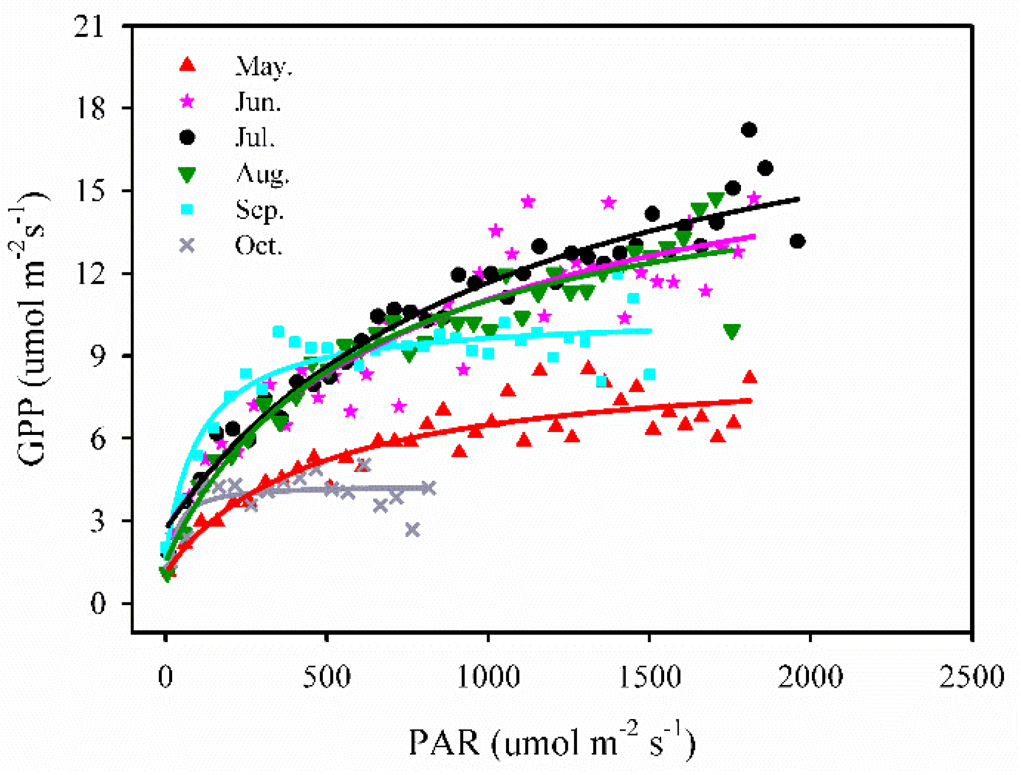
We employed a simple, rectangular hyperbolae (Michaelis-Menten) model [41] to analyze the relationship between daily PAR and GPP by each month, whereas the data points of GPP were averaged in 50 μ mol m−2 s−1 PAR bins. This relationship was described by the equation:
where GPP is the gross primary production, PAR is photosynthetically active radiation, Amax is a maximum rate of photosynthesis, K is the Michaelis-Menten constant, and Rd is a respiratory term. The coefficient of variation (R2) values were very high during May to September, ranging from 0.84 to 0.95.
From the period May to August, GPP increased linearly with an increase in PAR at the beginning of the period and then, it stabilized gradually when the PAR values reached around 800 μ mol m−2 s−1 for the month of May and around 1000–1200 μ mol m−2 s−1 for the months of June–August. Then the GPP showed a low and quick increase with PAR, and the maximum GPP was found to be approximately 8.5 μ mol m−2 s−1 in May. In the period of September and October, the maximum GPP values were found to be approximately 12 μ mol m−2 s−1 and 5 μ mol m−2 s−1, respectively. It is evident that the saturating response of GPP to PAR was different between the leaf emergence (in May), the vibrant growing period (from June to August, that was similar among those months) and leaf senescence period (from September to October) (Figure 8).
4. Discussion
4.1. CO2 Fluxes in the Riparian Forest
Riparian vegetation is an integral component of riparian zones (such as studied in this paper), thus it is vital to maintain a number of key environmental services in these important zones [42]. With potential access to groundwater, the riparian ecosystems maintain a higher level of biodiversity and productivity compared to the surrounding desert environment [23,24]. However, there have been only a few studies that have focused on the carbon sink of riparian forests and their environmental control mechanisms. The riparian forest in this study was found to be an important carbon sink, with an average NEP of 334 g C m−2 year−1. This value is comparable with the riparian cottonwood (Populus fremontii S. Watson) forest found in northern California’s Central Valley (i.e., 310 g C m−2 year−1) [23] and the riparian mesquite woodland situated along the San Pedro River in southeastern Arizona (i.e., 233 g C m−2 year−1) [24], USA. By contrast, the Poplar (i.e., Populus sp.) plantations in northern China with the GWD value of up to 15 m was a strong carbon sink [21], in which the NEP (720 g C m−2 year−1) was remarkably higher than that of the riparian forest [23,24] mentioned above and in this study. The productivity of riparian forest was primarily controlled by the presence of groundwater [23,24], as discussed in greater detail in the next section.
4.2. Controls on the Carbon Fluxes of Riparian Forest
Ecosystem NPP is widely known to be controlled by meteorological and hydrological regimes. Given the similar meteorological variables except precipitation (Table 1), we suggest the temporal pattern of CO2 fluxes of the riparian forest was mainly controlled by the soil hydrological regime including precipitation and groundwater. Liu et al. [43] showed that the aboveground NPP of riparian and desert vegetation in the middle HRB was strongly associated with annual precipitation. However, we found that the annual precipitation was not related to the CO2 fluxes of riparian forest due to the paucity of rainfall in the hyper-arid region within the lower HRB. Since it was demonstrated that the higher P (i.e., 52.1 mm, 2016) corresponded to the lowest NEP (278 g C m−2 year−1), and conversely, the lowest P (17.3 mm, 2014) corresponded to the second lower NEP (297 g C m−2 year−1) (Table 1), this data may suggest that the annual precipitation could not be used to explain the year-to-year variations in CO2 fluxes.
In search for plausible explanations, one could consider that for a single rainfall event, the maximum precipitation at the site is likely to be less than 9 mm, and therefore, the water cannot reach the soil layer of 60 cm, where is the primarily distributed range of fine roots of the dominant forests [44]. And some larger diameter roots are likely to be distributed below the groundwater depth level in this study site [44]. Deep rooting can thus reach the groundwater and thus redistribute such waters into the upper soil profile, enabling the tree to utilize both water sources [8,44], so that the riparian forest can grow continuously under hyper-arid climates. In fact, some studies have shown that the annual precipitation could not explain the inter-annual variations of CO2 fluxes in arid ecosystems [45,46], which has also been confirmed by the present study.
In the present study area, the soil textures were generally coarse, and the salt content was high and concentrated on the surface (Figure 4). In this regard, the salinization issues are considerably serious. In addition, the salinity of the groundwater was high, and this varied from about 800 to 3000 mg L−1 [47]. After decades of ecological water conveyance in this study region, the groundwater depth has become quite shallow and exhibits significant fluctuations, resulting in the accumulation of salts in the ground water and the surface soils [48]. The groundwater and salinity can both synthetically affect the growth of the desert riparian forests. Indeed, the study of Wang et al. [48] indicated that the accumulation of salinity is likely to offset the vegetation restoration process that could happen due to alleviated water stress, through the increase in the salt stress to plants.
In this study, the groundwater depth fluctuated from 0.28 to 2.42 m within the three years of the observation period. In fact, the values were well above the rational depth (i.e., 3.5–4.5 m) for the growth of P. euphratica [49] and the critical depth of ground water which was greater than 5 m. During the growing season, evapotranspiration is normally intensive due to the extremely dry climate, thus the changes in groundwater depth are likely to directly affect the accumulation of surface salinity that could eventually lead to the disturbance of the growth and development of the riparian forest. This is because the shallower is the groundwater depth, the greater is the evapotranspiration and the more serious is the soil salinization.
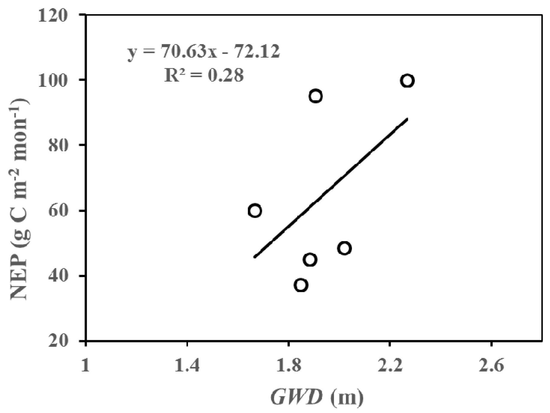
In this part, we analyzed the inter-annual differences in net ecosystem productivity (NEP) at different growing stages (at monthly scale) according to Figure 3 and Figure 6, and discussed possible reasons causing these differences. We suggested that the salinity of soil may be one of the significant factors influencing the growth of the riparian forest. From Figure 3 and Figure 6, we can directly and apparently obtain the following results: (1) Lower NEP values were accompanied by deeper GWD at the early phase of the growing season (i.e., May and June). More specifically, lower NEP and deeper groundwater values were found in May and June of 2015 compared to those in 2014 and 2016. Two plausible reasons for this result were as follows: firstly, the benefits of an increase in available water are expected to weaken the detrimental impacts of the accumulation of salinity in the forests at the early growing stage; secondly, less salinity accumulation occurred in this stage because of relatively small evapotranspiration. (2) The shallower groundwater depth corresponded to lower NEP in the vibrant growing season (i.e., July and August). These results could also be shown from Figure 9. As such, the NEP values in July and August 2015 were higher compared to those in 2014 and 2016. The soil capillary water can be more active with the higher Ta and the strongest evapotranspiration, such that, the shallower is the GWD, the greater is the accumulation of salinity in the soils (Figure 4). (3) In the late growing season, the groundwater depth in 2015 (i.e., 2 m) was deeper than that in 2014 (i.e., 0.6 m) and 2016 (i.e., 0.4 m). Therefore, the differences caused by temperature could be ignored. As a result, the NEP in September and October of 2015 was found to be much higher than that in 2014 and 2016. Consequently, the growth of the riparian forests is expected to be affected by the salinity in two main aspects [50,51,52]: Firstly, increased soluble salt ions in the soils can lead to a higher osmotic pressure, and a reduction in the soil water availability, which could inhibit the trees’ growth. Secondly, the salt ions that enter into the plant and then accumulate with the loss of water likely reduce the physiological metabolism in the plant. In conclusion, the inter-annual variations in NEP were pronounced, and may be driven by temperature and groundwater depth under similar eco-physiological process.
5. Conclusions
The study has demonstrated that P. euphratica forest is a considerable carbon sink in hyper-arid regions, with an average NEP of 334 g C m−2 year−1, which is comparable to levels of other riparian forests. The seasonal and inter-annual variations in NEP were mostly driven by temperature and groundwater depth under similar eco-physiological processes, which were significantly correlated with the Ta, PAR, VPD and Ep. Moreover, the inter-annual variation wherein annual NEP was lower due to higher temperatures and shallower groundwater depth in 2014 and 2016, was likely to be controlled by groundwater, since there were similar meteorological variables among the years. Finally, we demonstrated that accumulation of salinity was likely to occur with higher temperatures and shallower groundwater depths, thus affecting the growth of the desert riparian forest.
Supplementary Materials
The following are available online at www.mdpi.com/1999-4907/8/10/379/s1, Table S1: Monthly change of climatic variables included the mean (Tmean, °C), maximum (Tmax, °C), minimum (Tmin, °C) of air temperature, precipitation (P, mm), relative humidity (RH, %), sunshine duration (Sd, hours), wind speed (U, m s−1) and pan evaporation (Ep, mm) at Ejin station during the past 60 years (1957–2016).
Acknowledgments
This work was funded by the National Natural Science Foundation of China (No. 31370466, No. 41401033 and No. 31370467). This work also was supported by the Key Research Program of Frontier Sciences, CAS (QYZDJ-SSW-DQC031). The authors thank anonymous referees for their reading of this manuscript and helpful reviews and comments.
Author Contributions
Xiaohong Ma analyzed data and wrote the paper; Qi Feng conceived the study; Tengfei Yu collected data and revised the paper; Yonghong Su and Ravinesh Deo revised the final paper.
Conflicts of Interest
The authors declare that they have no conflict of interest.
References
- Le Quéré, C.; Andres, R.J.; Boden, T.; Conway, T.; Houghton, R.A.; House, J.I.; Marland, G.; Peters, G.P.; van der Werf, G.R.; Ahlström, A.; et al. The global carbon budget 1959–2011. Earth Syst. Sci. Data 2013, 5, 165–185. [Google Scholar] [CrossRef] [Green Version]
- Friedlingstein, P.; Meinshausen, M.; Arora, V.K.; Jones, C.D.; Anav, A.; Liddicoat, S.K.; Knutti, R. Uncertainties in CMIP5 climate projections due to carbon cycle feedbacks. J. Clim. 2014, 27, 511–526. [Google Scholar] [CrossRef]
- Schaphoff, S.; Lucht, W.; Gerten, D.; Sitch, S.; Cramer, W.; Prentice, I.C. Terrestrial biosphere carbon storage under alternative climate projections. Clim. Chang. 2006, 74, 97–122. [Google Scholar] [CrossRef]
- Ahlström, A.; Raupach, M.R.; Schurgers, G.; Smith, B.; Arneth, A.; Jung, M.; Reichstein, M.; Canadell, J.G.; Friedlingstein, P.; Jain, A.K. The dominant role of semi-arid ecosystems in the trend and variability of the land CO2 sink. Science 2015, 348, 895–899. [Google Scholar] [CrossRef] [PubMed]
- Poulter, B.; Frank, D.; Ciais, P.; Myneni, R.B.; Andela, N.; Bi, J.; Broquet, G.; Canadell, J.G.; Chevallier, F.; Liu, Y.Y.; et al. Contribution of semi-arid ecosystems to interannual variability of the global carbon cycle. Nature 2014, 509, 600–603. [Google Scholar] [CrossRef] [PubMed]
- Hao, X.M.; Li, W.H.; Huang, X.; Zhu, C.G.; Ma, J.X. Assessment of the groundwater threshold of desert riparian forest vegetation along the middle and lower reaches of the Tarim river, China. Hydrol. Process. 2009. [Google Scholar] [CrossRef]
- Li, W.H.; Zhou, H.H.; Fu, A.H.; Chen, Y.P. Ecological response and hydrological mechanism of desert riparian forest in Inland River, northwest of China. Ecohydrology 2013, 6, 949–955. [Google Scholar] [CrossRef]
- Si, J.H.; Feng, Q.; Cao, S.; Yu, T.F.; Zhao, C.Y. Water use sources of desert riparian Populus euphratica forests. Environ. Monit. Assess. 2014, 186, 5469–5477. [Google Scholar] [CrossRef] [PubMed]
- Smith, S.D.; Huxman, T.E.; Zitzer, S.F.; Charlet, T.N.; Housman, D.C.; Coleman, J.S.; Fenstermaker, L.K.; Seemann, J.R.; Nowak, R.S. Elevated CO2 increases productivity and invasive species success in an arid ecosystem. Nature 2000, 408, 79–82. [Google Scholar] [CrossRef] [PubMed]
- Curtis, P.S.; Hanson, P.J.; Bolstad, P.; Barford, C.; Randolph, J.C.; Schmid, H.P.; Wilson, K.B. Biometric and eddy-covariance based estimates of annual carbon storage in five eastern North American deciduous forests. Agric. For. Meteorol. 2002, 113, 3–19. [Google Scholar] [CrossRef]
- Baldocchi, D.D.; Vogel, C.A.; Hall, B. Seasonal variation of carbon dioxide exchange rates above and below a boreal jack pine forest. Agric. For. Meteorol. 1997, 83, 147–170. [Google Scholar] [CrossRef]
- Baldocchi, D.D. Assessing the eddy covariance technique for evaluating carbon dioxide exchange rates of ecosystems: Past, present and future. Glob. Chang. Biol. 2003, 9, 479–492. [Google Scholar] [CrossRef]
- Hirata, R.; Hirano, T.; Saigusa, N.; Fujinuma, Y.; Inukai, K.; Kitamori, Y.; Takahashi, Y.; Yamamoto, S. Seasonal and interannual variations in carbon dioxide exchange of a temperate larch forest. Agric. For. Meteorol. 2007, 147, 110–124. [Google Scholar] [CrossRef]
- Schimel, D.S.; House, J.I.; Hibbard, K.A.; Bousquet, P.; Ciais, P.; Peylin, P.; Braswell, B.H.; Apps, M.J.; Baker, D.; Bondeau, A.; et al. Recent patterns and mechanisms of carbon exchange by terrestrial ecosystems. Nature 2001, 414, 169–172. [Google Scholar] [CrossRef] [PubMed]
- Amiro, B.D.; Barr, A.G.; Barr, J.G.; Black, T.A.; Bracho, R.; Brown, M.; Chen, J.; Clark, K.L.; Davis, K.J.; Desai, A.R.; et al. Ecosystem carbon dioxide fluxes after disturbance in forests of North America. J. Geophys. Res. 2010, 115. [Google Scholar] [CrossRef]
- Williams, C.A.; Gu, H.; MacLean, R.; Masek, J.G.; Collatz, G.J. Disturbance and the carbon balance of us forests: A quantitative review of impacts from harvests, fires, insects, and droughts. Glob. Planet. Chang. 2016, 143, 66–80. [Google Scholar] [CrossRef]
- Ziemblińska, K.; Urbaniak, M.; Chojnicki, B.H.; Black, T.A.; Niu, S.; Olejnik, J. Net ecosystem productivity and its environmental controls in a mature scots pine stand in Northwestern Poland. Agric. For. Meteorol. 2016, 228–229, 60–72. [Google Scholar] [CrossRef]
- Houghton, R.A.; Skole, D.L.; Nobre, C.A.; Hackler, J.L.; Lawrence, K.T.; Chomentowski, W.H. Annual fluxes of carbon from deforestation and regrowth in the Brazilian Amazon. Nature 2000, 403, 301–304. [Google Scholar] [CrossRef] [PubMed]
- Ma, X.L.; Huete, A.; Cleverly, J.; Eamus, D.; Chevallier, F.; Joiner, J.; Poulter, B.; Zhang, Y.; Guanter, L.; Meyer, W.; et al. Drought rapidly diminishes the large net CO2 uptake in 2011 over Semi-Arid Australia. Sci. Rep. 2016, 6, 37747. [Google Scholar] [CrossRef] [PubMed]
- Kutsch, W.L.; Hanan, N.; Scholes, R.J.; Mchugh, I.; Kubheka, W.; Eckhardt, H.; Williams, C. Response of carbon fluxes to water relations in a savanna ecosystem in South Africa. Biogeosci. Discuss. 2008, 5, 2197–2235. [Google Scholar] [CrossRef]
- Zhou, J.; Zhang, Z.Q.; Sun, G.; Fang, X.R.; Zha, T.G.; McNulty, S.; Chen, J.Q.; Jin, Y.; Noormets, A. Response of ecosystem carbon fluxes to drought events in a poplar plantation in northern china. For. Ecol. Manag. 2013, 300, 33–42. [Google Scholar] [CrossRef]
- Garcia-Franco, N.; Wiesmeier, M.; Goberna, M.; Martínez-Mena, M.; Albaladejo, J. Carbon dynamics after afforestation of semiarid shrublands: Implications of site preparation techniques. For. Ecol. Manag. 2014, 319, 107–115. [Google Scholar] [CrossRef]
- Kochendorfer, J.; Castillo, E.G.; Haas, E.; Oechel, W.C.; Paw, U.K.T. Net ecosystem exchange, evapotranspiration and canopy conductance in a riparian forest. Agric. For. Meteorol. 2011, 151, 544–553. [Google Scholar] [CrossRef]
- Scott, R.L.; Huxman, T.E.; Williams, D.G.; Goodrich, D.C. Ecohydrological impacts of woody-plant encroachment: Seasonal patterns of water and carbon dioxide exchange within a semiarid riparian environment. Glob. Chang. Biol. 2006, 12, 311–324. [Google Scholar] [CrossRef]
- Feng, Q.; Cheng, G.D. Current situation, problems and rational utilization of water resources in arid Northwestern China. J. Arid Environ. 1998, 40, 373–382. [Google Scholar]
- Hou, L.G.; Xiao, H.L.; Si, J.H.; Xiao, S.C.; Zhou, M.X.; Yang, Y.G. Evapotranspiration and crop coefficient of Populus euphratica Oliv forest during the growing season in the extreme arid region Northwest China. Agric. Water Manag. 2010, 97, 351–356. [Google Scholar] [CrossRef]
- Feng, Q.; Peng, J.Z.; Li, J.G.; Xi, H.Y.; Si, J.H. Using the concept of ecological groundwater level to evaluate shallow groundwater resources in hyperarid desert regions. J. Arid Land 2012, 4, 378–389. [Google Scholar] [CrossRef]
- Xi, H.Y.; Feng, Q.; Si, J.H.; Chang, Z.Q.; Cao, S.K. Impacts of river recharge on groundwater level and hydrochemistry in the lower reaches of Heihe River watershed, Northwestern China. Hydrogeol. J. 2010, 18, 791–801. [Google Scholar] [CrossRef]
- Guo, Q.L.; Feng, Q.; Li, J.L. Environmental changes after ecological water conveyance in the lower reaches of Heihe River, Northwest China. Environ. Geol. 2009, 58, 1387–1396. [Google Scholar] [CrossRef]
- Wang, Y.; Feng, Q.; Chen, L.J.; Yu, T.F. Significance and effect of ecological rehabilitation project in Inland river basins in Northwest China. Environ. Manag. 2013, 52, 209–220. [Google Scholar] [CrossRef] [PubMed]
- Si, J.H.; Feng, Q.; Zhang, X.Y.; Chang, Z.Q.; Su, Y.H.; Xi, H.Y. Sap flow of Populus euphratica in a desert riparian forest in an extreme arid region during the growing season. J. Integr. Plant Biol. 2007, 49, 425–436. [Google Scholar] [CrossRef]
- Yu, T.F.; Feng, Q.; Si, J.H. Evapotranspiration of a Populus euphratica Oliv. forest and its controlling factors in the lower Heihe River basin, Northwest China. Sci. Cold Arid Reg. 2017, 9, 0175–0182. [Google Scholar]
- Moore, C.J. Frequency response corrections for eddy correlation systems. Bound.-Layer Meteorol. 1986, 37, 17–35. [Google Scholar] [CrossRef]
- Webb, E.K.; Pearman, G.I.; Leuning, R. Correction of flux measurements for density effects due to heat and water vapour transfer. Q. J. R. Meteorol. Soc. 1980, 106, 85–100. [Google Scholar] [CrossRef]
- Vickers, D.; Mahrt, L. Quality control and flux sampling problems for tower and aircraft data. J. Atmos. Ocean. Technol. 1997, 14, 512–526. [Google Scholar] [CrossRef]
- Papale, D.; Reichstein, M.; Aubinet, M.; Canfora, E.; Bernhofer, C.; Kutsch, W.; Longdoz, B.; Rambal, S.; Valentini, R.; Vesala, T.; et al. Towards a standardized processing of net ecosystem exchange measured with eddy covariance technique: Algorithms and uncertainty estimation. Biogeosciences 2006, 3, 571–583. [Google Scholar] [CrossRef]
- Reichstein, M.; Falge, E.; Baldocchi, D.; Papale, D.; Aubinet, M.; Berbigier, P.; Bernhofer, C.; Buchmann, N.; Gilmanov, T.; Granier, A.; et al. On the separation of net ecosystem exchange into assimilation and ecosystem respiration: Review and improved algorithm. Glob. Chang. Biol. 2005, 11, 1424–1439. [Google Scholar] [CrossRef]
- Fan, Y.; Li, H.; Miguez-Macho, G. Global patterns of groundwater table depth. Science 2013, 339, 940–943. [Google Scholar] [CrossRef] [PubMed]
- Li, Z.; Chen, Y.N.; Shen, Y.J.; Liu, Y.B.; Zhang, S.H. Analysis of changing pan evaporation in the arid region of Northwest China. Water Resour. Res. 2013, 49, 2205–2212. [Google Scholar] [CrossRef]
- Valentini, R.; Matteucci, G.; Dolman, A.J.; Schulze, E.D.; Rebmann, C.; Moors, E.J.; Granier, A.; Gross, P.; Jensen, N.O.; Pilegaard, K.; et al. Respiration as the main determinant of carbon balance in European forests. Nature 2000, 404, 861–865. [Google Scholar] [CrossRef] [PubMed]
- Hollinger, D.Y.; Goltz, S.M.; Davidson, E.A.; Lee, J.T.; Tu, K.; Valentine, H.T. Seasonal patterns and environmental control of carbon dioxide and water vapour exchange in an ecotonal boreal forest. Glob. Chang. Biol. 1999, 5, 891–902. [Google Scholar] [CrossRef]
- O’Grady, A.; Eamus, D.; Cook, P.; Lamontagne, S. Comparative water use by the riparian trees Melaleuca argentea and Corymbia bella in the wet-dry tropics of northern Australia. Tree Physiol. 2006, 26, 219–228. [Google Scholar] [CrossRef] [PubMed]
- Liu, B.; Guan, H.D.; Zhao, W.Z.; Yang, Y.T.; Li, S.B. Groundwater facilitated water-use efficiency along a gradient of groundwater depth in arid Northwestern China. Agric. For. Meteorol. 2017, 233, 235–241. [Google Scholar] [CrossRef]
- Yu, T.F.; Feng, Q.; Si, J.H.; Xi, H.Y.; Li, Z.X.; Chen, A.F. Hydraulic redistribution of soil water by roots of two desert riparian phreatophytes in Northwest China’s extremely arid region. Plant Soil 2013, 372, 297–308. [Google Scholar] [CrossRef]
- Jia, X.; Zha, T.S.; Gong, J.N.; Wang, B.; Zhang, Y.Q.; Wu, B.; Qin, S.G.; Peltola, H. Carbon and water exchange over a temperate semi-arid shrubland during three years of contrasting precipitation and soil moisture patterns. Agric. For. Meteorol. 2016, 228–229, 120–129. [Google Scholar] [CrossRef]
- Biederman, J.A.; Scott, R.L.; Goulden, M.L.; Vargas, R.; Litvak, M.E.; Kolb, T.E.; Yepez, E.A.; Oechel, W.C.; Blanken, P.D.; Bell, T.W.; et al. Terrestrial carbon balance in a drier world: The effects of water availability in Southwestern North America. Glob. Chang. Biol. 2016, 22, 1867–1879. [Google Scholar] [CrossRef] [PubMed]
- Wei, L.; Tao, W.; Hong, S.Y.; Hua, S.J.; Wu, Z.Y.; Qiang, C.Z. Analysis of the characteristics of soil and groundwater salinity in the lower reaches of Heihe river. J. Glaciol. Geocryol. 2005, 27, 890–898. [Google Scholar]
- Wang, P.; Zhang, Y.C.; Yu, J.J.; Fu, G.B.; Ao, F. Vegetation dynamics induced by groundwater fluctuations in the lower Heihe river basin, Northwestern China. J. Plant Ecol. 2011, 4, 77–90. [Google Scholar] [CrossRef]
- Chen, Y.N.; Pang, Z.H.; Chen, Y.P.; Li, W.H.; Xu, C.; Hao, X.M.; Huang, X.; Huang, T.M.; Ye, Z.X. Response of riparian vegetation to water-table changes in the lower reaches of Tarim river, Xinjiang Uygur, China. Hydrogeol. J. 2008, 16, 1371–1379. [Google Scholar] [CrossRef]
- Chen, S.L.; Li, J.K.; Wang, S.S.; Hüttermann, A.; Altman, A. Salt, nutrient uptake and transport, and aba of Populus euphratica; a hybrid in response to increasing soil NACL. Trees 2001, 15, 186–194. [Google Scholar] [CrossRef]
- Zeng, F.J.; Yan, H.L.; Arndt, S.K. Leaf and whole tree adaptations to mild salinity in field grown Populus euphratica. Tree Physiol. 2009, 29, 1237–1246. [Google Scholar] [CrossRef] [PubMed]
- Rajput, V.D.; Minkina, T.; Yaning, C.; Sushkova, S.; Chapligin, V.A.; Mandzhieva, S. A review on salinity adaptation mechanism and characteristics of Populus euphratica, a boon for arid ecosystems. Acta Ecol. Sin. 2016, 36, 497–503. [Google Scholar] [CrossRef]
Figure 1.
The schematic diagram of the Heihe River Basin (HRB), selected Populus euphratica stand and Ejin Meteorological Station, northwest China.
Figure 1.
The schematic diagram of the Heihe River Basin (HRB), selected Populus euphratica stand and Ejin Meteorological Station, northwest China.
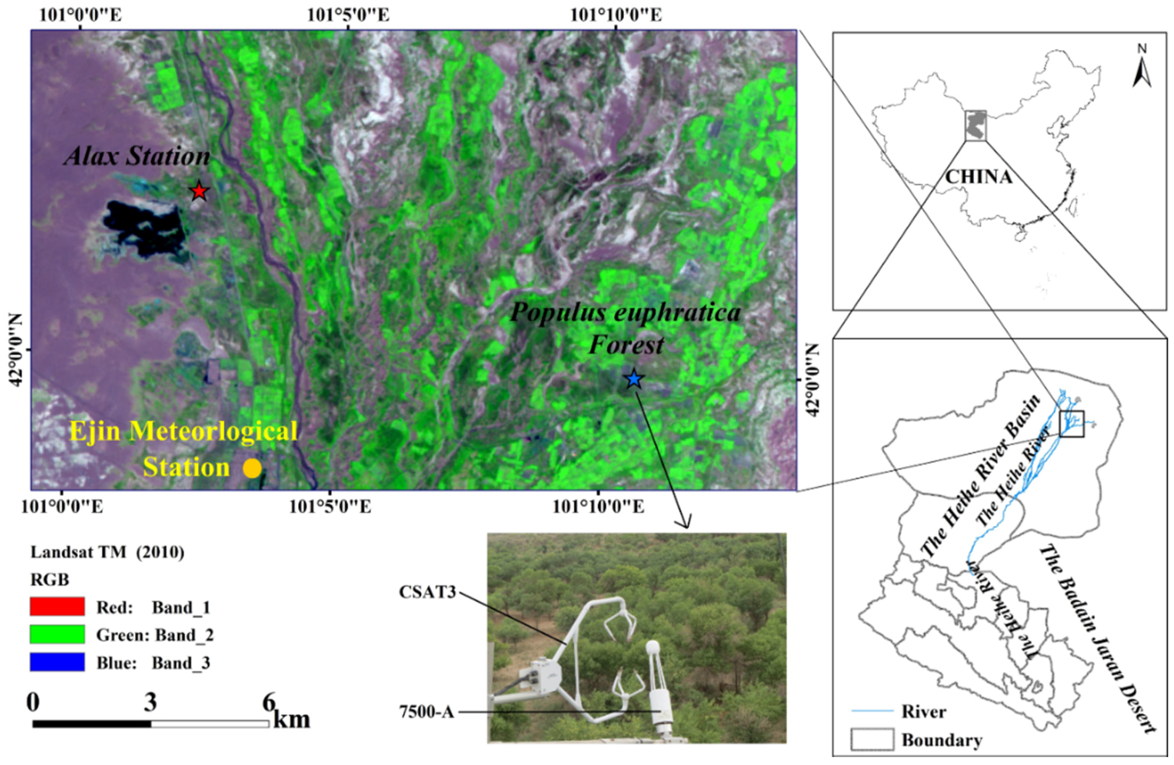
Figure 2.
A matrix of annual mean (±S.D., vertical bars) air temperature (Ta) and the annual precipitation (P) for the study period 2013–2016 at the lower reach of Heihe River Basin. The vertical and horizontal lines are the mean annual Ta and P (1957–2016), respectively.
Figure 2.
A matrix of annual mean (±S.D., vertical bars) air temperature (Ta) and the annual precipitation (P) for the study period 2013–2016 at the lower reach of Heihe River Basin. The vertical and horizontal lines are the mean annual Ta and P (1957–2016), respectively.

Figure 3.
Seasonal patterns of groundwater depth (GWD), air temperature (Ta), relative humidity (RH) and pan evaporation (Ep) data at the study site. The solid lines indicate the monthly mean values for the period 1957–2016.
Figure 3.
Seasonal patterns of groundwater depth (GWD), air temperature (Ta), relative humidity (RH) and pan evaporation (Ep) data at the study site. The solid lines indicate the monthly mean values for the period 1957–2016.

Figure 4.
Seasonal variations of the daily: (a) soil moisture content (θ, %), and (b) electrical conductivity (EC, mS cm−1) for P. euphratica stand for the period 2015–2016.
Figure 4.
Seasonal variations of the daily: (a) soil moisture content (θ, %), and (b) electrical conductivity (EC, mS cm−1) for P. euphratica stand for the period 2015–2016.
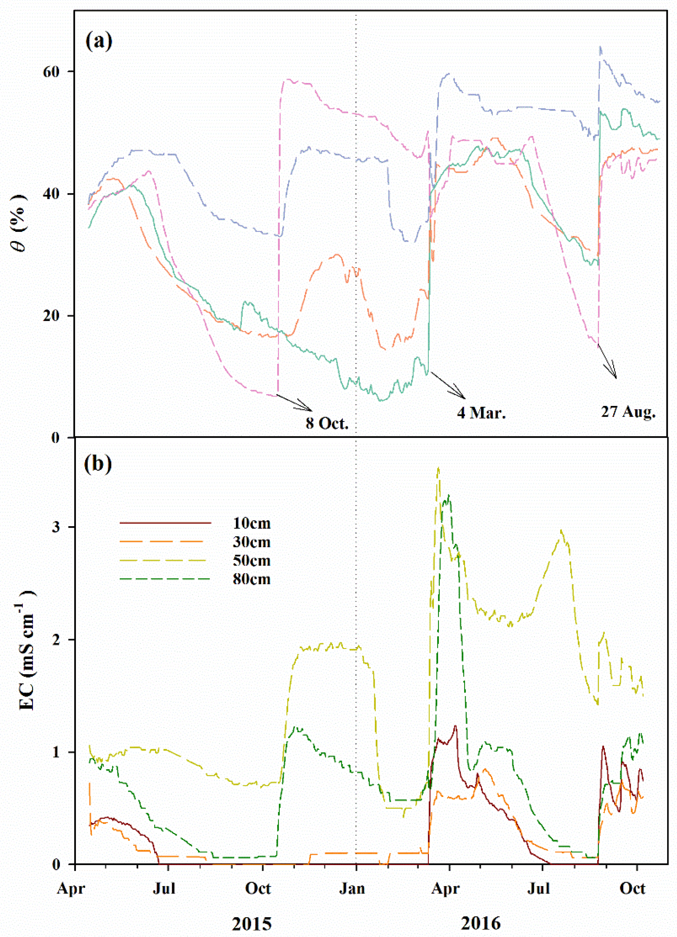
Figure 5.
Seasonal and inter-annual variations of net ecosystem exchange (NEE), gross primary production (GPP) and ecosystem respiration (Re) in 2013–2016 at the study site. Solid lines represent the variations of daily carbon fluxes, and dots represent the ten-day means.
Figure 5.
Seasonal and inter-annual variations of net ecosystem exchange (NEE), gross primary production (GPP) and ecosystem respiration (Re) in 2013–2016 at the study site. Solid lines represent the variations of daily carbon fluxes, and dots represent the ten-day means.

Figure 6.
Monthly totals of C balance components: (a) net ecosystem productivity (NEP), (b) gross primary production (GPP), and (c) ecosystem respiration (Re) at the study site. The solid lines indicate mean values of NEP, GPP and Re for 2013–2016.
Figure 6.
Monthly totals of C balance components: (a) net ecosystem productivity (NEP), (b) gross primary production (GPP), and (c) ecosystem respiration (Re) at the study site. The solid lines indicate mean values of NEP, GPP and Re for 2013–2016.
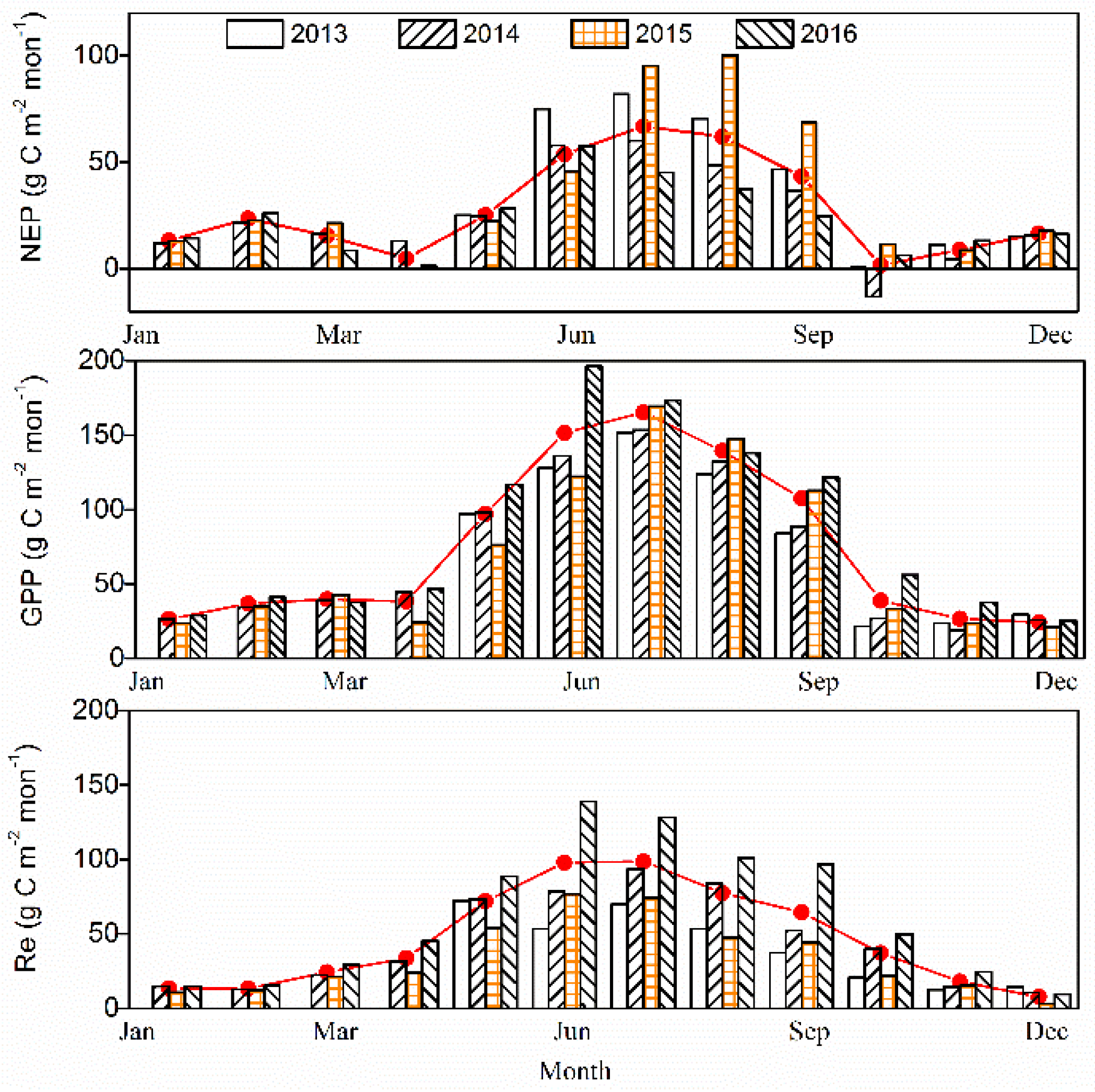
Figure 7.
The relationship between raw half-hourly nighttime NEE (Renight) and soil temperature (Ts) data at the study site. Data of Renight used in curve fitting were averaged in 0.2 °C Ts bins.
Figure 7.
The relationship between raw half-hourly nighttime NEE (Renight) and soil temperature (Ts) data at the study site. Data of Renight used in curve fitting were averaged in 0.2 °C Ts bins.
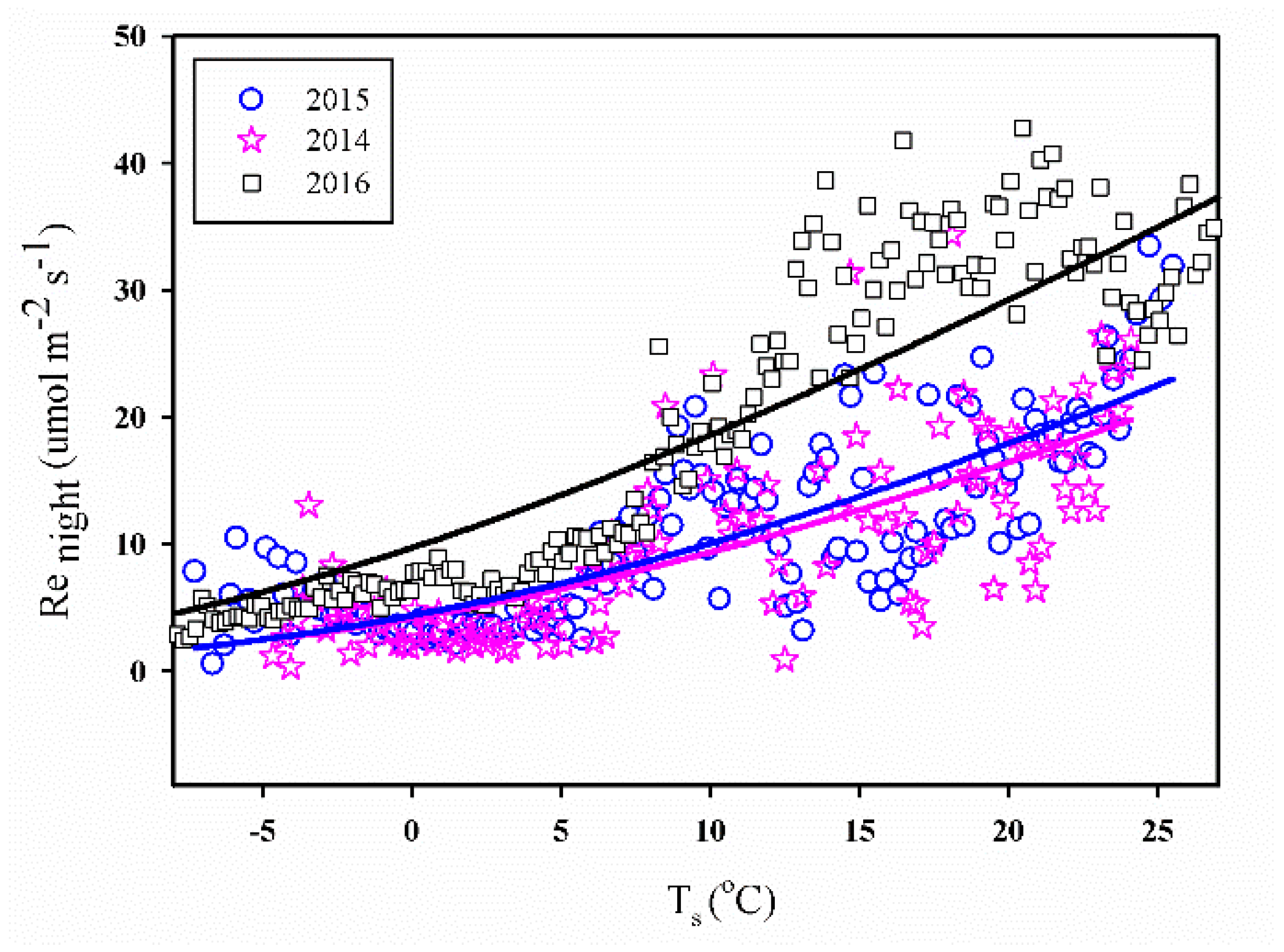
Figure 8.
Responses of gross primary production (GPP) to photosynthetically active radiation (PAR) from May to October across two years, 2015–2016, at the study site. GPP used in curve fitting was averaged in 50 μ mol m−2 s−1 PAR bins.
Figure 8.
Responses of gross primary production (GPP) to photosynthetically active radiation (PAR) from May to October across two years, 2015–2016, at the study site. GPP used in curve fitting was averaged in 50 μ mol m−2 s−1 PAR bins.

Figure 9.
The relationship between net ecosystem productivity (NEP) and groundwater depth (GWD) in July and August across three years (2014–2016) at the study site.
Figure 9.
The relationship between net ecosystem productivity (NEP) and groundwater depth (GWD) in July and August across three years (2014–2016) at the study site.


Table 1.
Yearly net ecosystem production (NEP), gross primary production (GPP), ecosystem respiration (Re), and mean GPP/Re in 2013–2016 at the study site. Also shown are mean air temperature (Ta), annual precipitation (P), and groundwater depth (GWD) during the growing season.
Table 1.
Yearly net ecosystem production (NEP), gross primary production (GPP), ecosystem respiration (Re), and mean GPP/Re in 2013–2016 at the study site. Also shown are mean air temperature (Ta), annual precipitation (P), and groundwater depth (GWD) during the growing season.
| Year | NEP | GPP | Re | GPP/Re | Ta | P | GWD |
|---|---|---|---|---|---|---|---|
| g C m−2 | °C | mm | m | ||||
| 2013 | 21.45 | 34.2 | 1.67 | ||||
| 2014 | 297 | 825 | 528 | 1.56 | 21.30 | 17.3 | 1.28 |
| 2015 | 427 | 834 | 405 | 2.05 | 20.98 | 70.1 | 1.79 |
| 2016 | 278 | 1019 | 742 | 1.37 | 21.46 | 52.1 | 1.16 |
| Average | 334 | 892 | 558 | 1.66 | 21.30 | 43.3 | 1.41 |
Table 2.
Spearman’s correlations between daily net ecosystem production (NEP, g C m−2 d−1), gross primary production (GPP, g C m−2 d−1) and ecosystem respiration (Re, g C m−2 d−1), and mean air temperature (Ta, °C), vapor pressure deficit (VPD, kPa), photosynthetically active radiation (PAR, μ mol m−2 s−1), groundwater depth (GWD, m) and pan evaporation (Ep, mm) during the growing season (from May to October) across four years, 2013–2016, at the study site.
| Ta | VPD | PAR | GWD | Ep | |
|---|---|---|---|---|---|
| NEP | 0.598 ** | 0.333 ** | 0.395 ** | 0.525 ** | 0.268 ** |
| GPP | 0.663 ** | 0.524 ** | 0.426 ** | 0.390 ** | 0.458 ** |
| Re | 0.457 ** | 0.538 ** | 0.100 | 0.079 | 0.504 ** |
** Correlation is significant at the 0.01 level (2-tailed).
© 2017 by the authors. Licensee MDPI, Basel, Switzerland. This article is an open access article distributed under the terms and conditions of the Creative Commons Attribution (CC BY) license (http://creativecommons.org/licenses/by/4.0/).
Share and Cite
MDPI and ACS Style
Ma, X.; Feng, Q.; Yu, T.; Su, Y.; Deo, R.C. Carbon Dioxide Fluxes and Their Environmental Controls in a Riparian Forest within the Hyper-Arid Region of Northwest China. Forests 2017, 8, 379. https://doi.org/10.3390/f8100379
AMA Style
Ma X, Feng Q, Yu T, Su Y, Deo RC. Carbon Dioxide Fluxes and Their Environmental Controls in a Riparian Forest within the Hyper-Arid Region of Northwest China. Forests. 2017; 8(10):379. https://doi.org/10.3390/f8100379
Chicago/Turabian StyleMa, Xiaohong, Qi Feng, Tengfei Yu, Yonghong Su, and Ravinesh C. Deo. 2017. "Carbon Dioxide Fluxes and Their Environmental Controls in a Riparian Forest within the Hyper-Arid Region of Northwest China" Forests 8, no. 10: 379. https://doi.org/10.3390/f8100379
Note that from the first issue of 2016, this journal uses article numbers instead of page numbers. See further details here.