Functional Response Trait Analysis Improves Climate Sensitivity Estimation in Beech Forests at a Trailing Edge


1
Institute of Biology, University of Pécs, Ifjúság útja, 6, 7624 Pécs, Hungary
2
Institute of Economics and Econometrics, Faculty of Business and Economics, University of Pécs, Rákóczi út 80, 7622 Pécs, Hungary
3
Institute of Biology, University of Pécs, Ifjúság útja, 6, 7624 Pécs, Hungary
*
Author to whom correspondence should be addressed.
Forests 2017, 8(9), 324; https://doi.org/10.3390/f8090324
Submission received: 15 July 2017
/
Revised: 25 August 2017
/
Accepted: 27 August 2017
/
Published: 31 August 2017
(This article belongs to the Special Issue New Insights into Climate Sensitivity of Forest Growth, Health, and Disturbance: Vulnerability, Resilience, and Change)
Abstract
:Functional response traits influence the ability of species to colonize and thrive in a habitat and to persist under environmental challenges. Functional traits can be used to evaluate environment-related processes and phenomena. They also help to interpret distribution patterns, especially under limiting ecological conditions. In this study, we investigate landscape-scale functional distribution responses of beech forests in a climatic transitional zone in Europe. We construct empirical density distribution responses for beech forests by applying coping-resilience-failure climatic traits based on 27 bioclimatic variables, resulting in prevalence-decay-exclusion distribution response patterns. We also perform multivariate exploratory cluster analysis to reveal significant sets of response patterns from the resilience and adaptation aspects. Temperature-related distribution responses presented a prevalence-dominated functional pattern, with Annual mean temperature indicating the most favorable adaptation function. Precipitation indices showed climate-limited response patterns with the dominance of extinction function. Considering regional site-specific climate change projections, these continental beech forests could regress moderately due to temperature increase in the near future. Our results also suggest that both summer and winter precipitation could play a pivotal role in successful resilience. Functions and variables that indicate climate sensitivity can serve as a useful starting point to develop adaptation measures for regional forest management.

1. Introduction
Functional traits are morphological, biochemical, physiological, structural, phenological or behavioral characteristics of organisms that influence performance or fitness, expressed by their phenotype. During the last three decades, the species-based trait concept has been generalized and interpreted at several levels ranging from populations to ecosystems [1,2,3]. This novel approach has been widely used in community and ecosystem ecology to define functional traits addressing the underlying concept that refers to [2,3,4,5,6]. In most cases, a trait is defined at the level of individuals, but the interpretation can be presented at any organizational level (e.g., community). Plant traits can frequently refer to ecological factors changing along a gradient, and researchers can present response traits for environmental resources or common disturbances. Functional response traits connected with an environmental gradient highlight the influence of the environment and the ability of a species to colonize and thrive in a habitat and to persist in the face of environmental changes [2,3]. A more frequent application of functional traits is to characterize community responses to environmental changes, focusing on quantification of community shifts by ecosystem processes that lead to functional diversity. However, the utility of these trait-based analyses in climate change research can particularly benefit from approaches that demonstrate how these traits or functions influence community and ecosystem processes [4,6]. Recently, there has been an increase in the number of ecological investigations to reveal relations between species-related functional traits and community-level processes connected by integration functions. Occurrence or frequency of a species can be reasonably interpreted as the inherent component of the response trait interpreted at community level resulting in the ecological performance of the community [1].
Adaptation can be defined as an adjustment of natural systems to a new or changing environment, in response to actual or expected climatic effects, which moderates harm or takes advantage of opportunities. This process refers to the ability or a response of an ecosystem to adjust ecological variation in order to enhance the resilience to observed or anticipated impacts of climate change [7]. Resilience and adaptation can inherently occur in natural ecosystems, primarily involving the perception or detection of climate exposure. Targeted research is necessary to study how forests respond to current and future environmental challenges. This is especially urgent for European forest stands, which possess high diversity and show regional differences. In temperate continental regions of Europe relatively few adaptation measures are being implemented, a majority of which are country specific or are still in the planning phase. Because of this, researchers should expand and develop adequate and site-specific implementation of adaptation options. A better understanding of opportunities is urgently needed in order to increase adaptive capacity and also to obtain a detailed regional sensitivity assessments of forest stands [8].
An operative concept related to climate change adaptation consists of three terms by critical thresholds that are used to define coping (C), resilience (R), and failure (F), as response function ranges [9,10]. Coping range represents the magnitude of disturbance (i.e., the variation in climatic stimuli) that an ecosystem can tolerate without significant adverse impacts. Resilience range refers to the magnitude of the damage that an ecosystem can tolerate, and from which it is able to return autonomously to its original state. Failure range starts from the point where the magnitude of damage is such, that a system can no longer tolerate it without significant adverse impacts. The variation in event severity (e.g., climate regime) in a system mainly depends on the magnitude of the coping and resilience ranges. In the presence of adaptation, coping and resilience ranges can be increased and failure range can be decreased or suppressed. Consequently, the above-mentioned CRF climate response assessment concept can help to evaluate environmental adaptation or resilience, and disturbance or sensitivity of the ecosystem. In order to evaluate environmental responses of species, communities or ecosystems, we list some key uncertainties and research needs. Climate response models can be improved by understanding the mechanism of climate impacts better, enhancing climate change impact assessment in areas with little or no previous investigations and continuing to study regional differences in adaptive capacity.
Temperature and precipitation are the most commonly used climatic factors that determine forest distribution at global, continental and regional scales. A continental-scale ecological analysis of the most important forest formations based on 56 environmental features including climatic and topographic variables suggested temperature-based indices to be the best predictors of distribution [11]. In this study, the authors suggested six characteristic temperature indices for hemiboreal forests; eight variables for subatlantic and subcontinental woodlands and nine temperature indices for the Pannonian-Pontic forest stands. Specifically, the distribution of montane beech forests was determined principally by non-climatic factors, such as altitude and bedrock composition. Similarly, the first-level division is supported by landscape-scale temperature gradient in the ecological classification of forests with European beech (Fagus sylvatica L.) [12].
Since temperature and precipitation perform in interaction, composite bioclimatic indices that contain both types of variables are even more promising analytical tools to reveal eco-climatic functions of species and ecosystems [13]. Climatic requirements of beech forests are characterized as temperate Atlantic climate with mild winters and moist summers [14]. Eight studies investigating the distribution limit of European beech forests found composite variables (temperature-related precipitation measures) to be significant climatic determinants, while six highlighted temperature-based variables and four pinpointed precipitation-related factors [15]. Temperature gradient closely followed by moisture proved to be the most important climatic predictor near the marginal occurrence of the distribution of European beech at the global scale, and regional differences were also indicated [16]. Low temperature (frost) in the winter, high temperature (heat) in June, and general drought throughout the year were also suggested as limiting factors in the growth of beech trees at the north-eastern edge of the European distribution [17]. In southeast Europe, beech dominated suballiances are differentiated by joined environmental factors, such as temperature and moisture [18]. Composite bioclimatic variables were found to be more important than precipitation measures to describe ecological variability of beech forests close to the xeric edge in southwest Hungary, but not the Ellenberg’s Quotient [19]. In general, drought indices (composites) are frequently used to discuss ecological assumptions of beech forests distribution throughout Europe [15,16,20,21,22,23].
Increasing frequency of extreme climate events and change in general conditions predicted by climate change scenarios, especially drought and heat, temperature and precipitation seasonality and variability all occur and are important in the Pannonian-Pontic region of Europe. Considering the complex ecological status of this region, climatic measures that reflect such processes and phenomena deserve attention [24,25]. While the distribution of hemiboreal forests cannot be characterized by any climate extremity variable, e.g., subcontinental beech forests reflect climate extremities, such as maximum and minimum temperature of coldest or warmest months or quarters [11].
European beech trees and forests are particularly affected by summer drought, as well as May and July temperatures, annual precipitation, and the temperature-to-rainfall ratio in the transitional forest-steppe vegetation zone [21], as well as in the Mediterranean-influenced regions [26]. Beech tree growth is consistently limited by high temperature and low precipitation during the growing season at the southern edge of the distribution [25,27]. At the same time, some authors draw attention to increased climate sensitivity of beech forests, due to the synergistic relation between extended growing season and increasing amount of atmospheric carbon dioxide in the Mediterranean region [28].
Beech forests and populations at the southern (Mediterranean) and eastern (continental) xeric distribution edge may be more vulnerable [20,25,29]. In addition, there are some contradicting studies on phenotypic and functional traits, including the landscape-scale distribution performance of beech forests. For instance, Romanian colline beech forests were found to be unaffected by climate fluctuation and change in general, however their growth was limited by June and September temperatures, and temperature-affected summer precipitation expressed by the Forestry Aridity Index [23]. Beech populations in dryer and warmer areas of Europe are genetically more adapted to drought that can mitigate their climatic exposure and vulnerability [15,30]. Moreover, beech populations are often reported to be drought resistant in Mediterranean regions. This drought resistance is obtained by physiological processes [31,32]. On the other hand, cold climate extremities also play an important role for individuals of Fagus sylvatica L. and also for forests. Among the important climatic predictors of species global occurrence, low winter temperature and high level of climatic continentality were found to be limiting [16]. Earlier studies reached similar conclusions for core distributional areas (e.g., [33,34]) and several currently marginal populations [17,26].
Given the diversified climatic relations of beech forest occurrence at the eastern and lowland limits of distribution, our objective was to present a functional response trait interpretation of distribution performance, primarily focusing on the trailing edge. Specifically, this study addressed: (1) the ecological variability of beech forests using various types of bioclimatic variables; (2) developing climatic response functions and measures derived from the coping-resilience-failure adaptation concept; and (3) estimating and selecting the most adequate climatic response traits that indicate resilience, adaptation and sensitivity of beech forests that exist in an ecologically diversified transitional landscape.
2. Materials and Methods
2.1. Site Description and Location
Our study area was the southern Transdanubian region, a hilly lowland landscape at the southern edge of the Pannonian Biogeographic Region (Figure 1) towards to the Mediterranean and semi-arid continental parts of Europe [35]. Elevation varies moderately between 79–610 m, orography is characterized by four rivers and the Lake Balaton, connected by a dense inland fluvial network. The main soil types are loess or loess-like, glacial and alluvial deposits, with sparse limestone or sandstone as parent material. Considering the climate reference period of 1961–1990, the annual precipitation is 648 mm, the mean annual temperature is 10.9 °C [36]. The study area is classified as temperate climatic zone at the intersection of three European macroclimatic regions: Oceanic, Continental, and Mediterranean [37]. This region is characterized as submontane oak-hornbeam woodlands of the thermo-nemoral domain by the large scale ecological mapping based on European vegetation units [13]. According to the updated Köppen-Geiger climate classification [38], it has cold humid continental climate with no arid season throughout the year.
At the regional scale, annual precipitation frequently shows a double maximum occurring in late spring and autumn that combined with warm or hot dry summers. Due to the influence of the Atlantic-Submediterranean macroclimate that interacts with the regional topography, a strong climatic gradient can be observed from the southwest towards the northeast of the region [37,39,40]. In particular, between June and August the period of the highest mean temperature overlaps with the period of the highest precipitation. Additionally, the period of the coldest quarter co-occurs with the driest quarter in the winter season, between January and March. Consequently, the ecological effect of the high summer temperature can largely be compensated by the high amount of precipitation, and also the winter season precipitation deficit can be balanced by the low temperature. The high resolution climatic and geographic heterogeneity in the study area is mainly resulted from the variability in precipitation.
2.2. Vegetation Survey and Beech Forests
The current natural vegetation of Hungary was systematically surveyed in 2004–2007, integrating geographical, landscape ecological, and land-use information [42]. Field data were collected using a systematic grid of 35-hectare hexagon-shaped spatial units, including vegetation records of beech forests. These data are managed in the MÉTA database [43]. The presence-absence data were embedded in the matrix of the regional sampling points consisting of any kind of natural habitat types (n = 39,450).
Beech forests in the study region are ‘Illyrian submontaneous beech forests’, belonging to the category ‘Beech forests’ of the recent European forest type classification system [44]. These stands belong to ‘91K0: Illyrian Fagus sylvatica forests (Aremonio-Fagion)’ according to the Natura 2000 habitat classification [18]. This habitat is equivalent to habitat ‘K5’ listed in the MÉTA database [45]. According to the current European syntaxonomic system of Fagus forests, occurrences can be classified into the Aremonio-Fagion alliance and are located the northwestern edge of its distribution [18]. In the national syntaxonomic system the stands can be classified into four associations: Vicio oroboidi-Fagetum Pócs & Borhidi 1960, Helleboro odori-Fagetum Soó & Borhidi in Soó 1960, Doronico austriaci-Fagetum Borhidi & Kevey 1996, Leucojo verni-Fagetum Kevey & Borhidi 1992 [46].
Illyrian beech forests occur at 123–606 m above the sea level in South Transdanubia (Figure 1). They cover about 12,000 ha with large extensions in the Zselic and Mecsek hills, and sporadically in the northern hilly parts of the region. Additionally, small relic stands occur along the Drava River on the lowlands. Forests stands are generally tall growing with a dense canopy layer (80–100% cover) at a height of 20–35 m with the monodominance (60–100%) of European beech. Associated tree species can be Carpinus betulus, Quercus petraea, Tilia tomentosa, Fraxinus excelsior, Sorbus torminalis. The shrub layer is missing or very sparse. The floristic composition of the understory is rich in characteristic mesic species, such as Actea spicata, Aremonia agrimonoides, Vicia oroboides, Primula acaulis, Knautia drymeia, Hepatica nobilis, Festuca drymeia, Cardamine enneaphyllos, Ruscus hypoglossum, Ruscus aculeatus, Lathyrus venetus and Tamus communis. Stands occur under wet or moist habitat conditions on calcareous bedrock, sometimes on moderately acidic soil [45,46]. We used the regional records of low-, and medium-elevated Illyrian beech forest stands referred to as ‘K5’ in the National Habitat Classification System [47]. We excluded records of sporadic occurrences of beech trees and beech forest stands under extraclimatic ecological conditions, such as those growing on acidophilous soil.
Beech forests in Hungary are managed in close-to-nature silviculture, forest regeneration is based on the natural regrowth. The majority of the stands are even-aged, the rotation period is 100–120 years. The new individuals appear under the canopy of old forest stands. Additionally, regeneration process is facilitated by creating a partial opening in the forest canopy (up to 20%) 5–10 years before the felling. As a consequence, present locations of forest stands are the same that it was in sixties or nineties.
2.3. Bioclimatic Variables
We used 27 bioclimatic (temperature, precipitation and composite) variables derived from the regional meteorological stations during the climate reference period of 1961–1990. Temperature values were imported from the WorldClim database [48,49]. Precipitation data were obtained from the Hungarian Meteorological Service as elevation-corrected spatially interpolated high-resolution climate surface data [36], using the AURELHY method (Analyse Utilisant le RELief pour l’HYdrométéorologie) as hydrometeorological interpolation including corrections with the local topography [50] after [51]. The topography is described at a range of scales by a Principal Component Analysis and weather station data were interpolated in a spatial linear model with the residuals krigged. We extracted central spatial coordinates to obtain climatic data for the hexagon grid system and acquired a systematic regional bioclimatic database.
We selected 17 temperature and precipitation indices from the BIOCLIM series corresponding to various time scales and definitions, e.g., monthly minimum, quarterly mean, annual variation [48,49]. We also used four ecologically powerful composite variables to emphasize temperature (e.g., Thermicity = Ti) and precipitation (e.g., Summer Drought Stress = SDS) variability or limitation in this transitional distribution zone. Moreover, six mixed composite indices (e.g., temperature and precipitation ratios) also proved to be useful to detect humidity-related climate function of the distribution (e.g., Compensated Summer Ombrothermic index = CSOi). Overall, 27 bioclimatic variables were used in the analyses (Table 1). The calculation methods of composite indices are presented in Equations (1)–(10).
Aridity index (Ai) [52]:
where Pann = annual precipitation; Tann = annual mean temperature; Pd and Td = mean temperature and precipitation of the driest month (here February); [mm °C−1].
Ai = [Pann/(Tann + 10) + 12 × Pd/(Td + 10)]/2,
Compensated Summer Ombrothermic index (CSOi) [53]:
where P05 to P08 = precipitation sum from May to August; T05 to T08 = sum of temperature means from May to August; [mm °C−1].
CSOi = (P05 + P06 + P07 + P08)/(T05 + T06 + T07 + T08),
Continentality index (Ci) [53]:
where Tmax h and Tmin c are the mean temperature of the hottest and the coldest months (July and January), respectively [°C].
Ci = Tmaxh − Tminc,
Ellenberg’s Quotient (EQ) [54]:
where Th = mean temperature of the hottest month (July); Pann = annual sum of precipitation; [°C mm−1].
EQ = 1000 × Th/Pann,
Forestry Aridity index (FAi) [55]:
where T07–08 = mean temperature of July and August; P05–07 = precipitation sum from May to July; P07–08 = precipitation sum from July to August; [°C mm−1].
FAi = 100 × (T07–08)/(P05–07 + P07–08),
Ombrothermic index (Oi) [53]:
where ΣPT0 = precipitation sum of the months with average temperature above 0 °C (February–December); ΣTT0 = mean temperature sum of months with average temperature above 0 °C (February–December); [mm °C−1].
Oi = 10 × (ΣPT0/ΣTT0),
Pluviothermic Quotient (Q) [56]:
where Pann = annual sum of precipitation; Tmaxh = mean of maximum temperature of the hottest month (July); Tminc = mean of minimum temperature of the coldest month (January); [mm °C−1].
Q = 2000 × Pann/(T2maxh − T2minc),
Summer Drought Stress (SDS) [57]:
where PS = mean precipitation of the three summer months (June–August); [mm].
SDS = 2 × (50 − Ps),
Thermicity index (Ti) [53]:
where Tann = annual mean temperature; Tminc and Tmaxc are the mean of minimum and maximum temperature of the coldest month (January); [°C].
Ti = 10 × (Tann + Tminc + Tmaxc),
Winter Cold Stress (WCS) [57]:
where Tmin_w = mean of minimum temperature of the winter months (December to February); [°C].
WCS = 8 × (10 − Tmin_w),
2.4. Data Processing and Analyses
First, we constructed an integrated regional database of the presence-absence records of beech forests and the 27 bioclimatic variables of all hexagonal sampling units. First, we performed an exploratory factor analysis (principal component extraction; Varimax normalized rotation; Eigenvalue > 1) on presence-only data of beech forest occurrences (n = 1868) in order to extract factors as principal components to identify the most important predictors of occurrences, and to detect independent sets of variables. We examined the factor loadings in the rotated component matrix to reveal the relative importance of each climatic variable.
Next, using all selected bioclimatic variables on presence-absence records of beech forests in the study area (n = 39,450), we performed a series of frequency distribution analyses. In the first step, we calculated relative observed frequency of beech forest distribution. Next, we computed the relative distribution of the geographic area using all bioclimatic variables to produce a reference frequency dataset. We assumed that beech forests distribution could be adjusted to any specified range of climatic conditions related to that of the region (but the exception of non-climatic factors). We also calculated a non-linear probability estimation of an area version of Gaussian multipeak model using least square method (NLSF) to construct probability response function. We applied the Levenberg-Marquard algorithm (LM) with a smooth approximation to conduct an iterative fitting procedure. We validated the statistical adequacy of curve fitting by the coefficient of determination (R2), and the empirical probability of the Chi-square value (p). The fitting process resulted in an integrated non-linear curve with an adequate set of Gaussians as modality.
2.5. Climatic Traits and Distribution Response Functions
In the next step, we used the curve fitting outcomes to calculate climatic trait ranges derived from the coping-resilience-failure concept [CRF]. Coping range [C] represents a response function meaning a tolerance without significant changes, i.e., the value where the integrated density curve of the forest exceeds that of the geographic area. Resilience range [R] indicates the magnitude of ecosystem response that can tolerate damages within; in our analysis it is indicated if the beech forest climate function response curve is subordinate to that of the region. Failure range [F] denotes the magnitude of the climatic response of an ecosystem that can no longer be tolerated without significant adverse effects. In our calculation, this climate response function is indicated by forest absence. Therefore, we calculated relative response trait functions [PDE] derived from the climatic trait ranges (Figure 2). Based on this, we calculated two specific response trait measures: Amplitude (A), which refers to the relative ratio sum of prevalence and decay functions (P + D), and Hardiness (H), which indicates the relative importance of prevalence function related to decay function (P/D). The higher the value of a response trait measure, the more favorable the state of resilience, leading to a more successful climate adaptation phenomenon. Starting with the primary data of CRF climatic trait ranges and the PDE response functions, we used these range-based measures to reveal adaptation phenomena of beech forests. Finally, we compiled a set of response trait functions and measures on all bioclimatic variables (Table 2).
We also constructed Receiving Operating Curves (ROC) with value of Area Under the Curve (AUC) to validate overall adaptation responses of beech forests for all bioclimatic variables. Receiver Operating Characteristic curve is one of the most widely used methods to analyze and present the separating power of a single variable between two sub-samples. The curve is constructed by calculating True positive rate (TPR) and False Positive Rate (FPR) that correspond with various threshold settings. Therefore, the proximity to the diagonal (i.e., a straight line at 45 degrees) derived from calculating the TPR to FPR ratio at various threshold settings indicates less predicting power of the variable. The AUC value is the most popular indicator measure of separating power. In case of a given variable, the higher the AUC value is, the more the beech forest can be separated from the functional distribution of the region. AUC = 0.5 means that the given variable has no predicting power, it is a completely random classifier. In our case, a low AUC value (close to 0.5) means that the distribution of beech forests is well-fitted to that of the region, due to the high prevalence and decay function ratio. On the other hand, high AUC value (well over 0.5) means that beech forests climate function is highly separated from that of the region, due to its low prevalence or/and decay function ratio. When AUC = 1.0, the variable can separate the sub-samples perfectly [58]. In our study we used the ROC analysis to calculate and compare the overall functional behavior of beech forests according to various types of bioclimatic indices (Table 1). Last, we applied joining (tree) clustering, a multivariate exploratory method, to discover structures in functional response traits that provide an interpretation of adaptation metric performance, using non-parametric tests (Mann-Whitney U-test and Kruskal-Wallis ANOVA) to identify significant differences between the clusters that contain sets of given extracted variables.
We used Microsoft Office Excel 2003 (Microsoft Corporation, Redmond, WA, USA) for frequency calculation, Origin 6.1 (OriginLab, Northampton, MA, USA) [59] for functional response curve computation, Statistica 12.6 (StatSoft Inc., Tulsa, OK, USA) [60] for statistical analyses (Factor Analysis, Tree Clustering, Kruskal-Wallis ANOVA, Mann-Whitney U-test), and R software package for ROC curve fitting and AUC calculation (The R Foundation, Vienna, Austria) [61].
3. Results
3.1. Climatic Variability of Beech Forests Distribution
Regarding beech forests presence-only data, the exploratory factor analysis resulted in four principal components based on the 27 bioclimatic variables (Table 1). In general, there was a high level of total variance (97.2%), partitioning in the first (PC-1; 69.0% variance; Eigenvalue: 18.6), second (PC-2; 17.4% variance; Eigenvalue: 4.7), third (PC-3; 6.1% variance; Eigenvalue: 1.6), and fourth (PC-4; 4.7% variance; Eigenvalue: 1.3) principal components. Our analysis extracted 11 important precipitation-related bioclimatic variables to describe climate-driven functional heterogeneity in the regional distribution pattern. The most important variable was the Annual precipitation (BIO12), while the Compensated Summer Ombrothermic index (CSOi) was interpreted to have the least importance. In this component in particular, variables with a specific precipitation-temperature ratio were subordinate in the interpretation of beech forests occurrence. The second component contained 12 separated temperature-derived variables, including Mean temperature of the coldest quarter (BIO11), which was the most important, and Ombrothermic index (Oi), which contributed minimally to this principal component. Three bioclimatic variables indicating seasonal or annual temperature variability were associated with the third principal component, essentially with the Continentality index (Ci). In the fourth principal component, one bioclimatic variable was extracted by Precipitation seasonality (BIO15) referring to the annual rainfall variation. Summarizing the relative importance of variables by factor loadings in all principal components, mean temperature during the winter season (January to March) and annual variability of precipitation proved to be the most important diversifying bioclimatic factors. Precipitation sum throughout the year and temperature difference between the coldest (January) and the hottest (July) months were subordinate for characterizing ecological heterogeneity.
3.2. Climatic Traits and Response Functions
Based on all regional plots including presence-absence records of beech forests, we constructed distribution-based climatic traits and functional responses (Figure 3 and Figure S1; Table 2). Disparity of the empirical distribution curves proved to be an appropriate tool to calculate PDE response functions from the CRF ranges of climatic traits. After range identification, we calculated the relative ratio of Prevalence (P), Decay (D), and Exclusion (E) response functions. Furthermore, two additional relative response trait measures, Amplitude (A) and Hardiness (H) were also developed for all bioclimatic variables. In total, these functional measures derived from climatic traits were compared in order to give a response-related interpretation of climate sensitivity and adaptation of studied beech forests.
Functional traits derived from variables in the first principal component provided a primary set to detect precipitation response functions of beech forests. Regarding all bioclimatic measures, prevalence response functions were generally detected under higher precipitation regimes. Compensated Summer Ombrothermic index (CSOi) had the highest ratio (52.5%) of prevalence range, and Annual precipitation (BIO12) had the lowest (25.2%). Resilience range (i.e., the decay response function of the distribution) was highly variable between Precipitation of the coldest quarter (BIO19) (36.8%) and Forestry Aridity index (FAi) (16.1%). Interestingly, decay range presented a continuous (uniform) response trait position for most bioclimatic variables, e.g., for Ellenberg’s Quotient (EQ), presenting the functional trailing edge of the distribution. On the other hand, some bioclimatic measures presented divided decay response functions, e.g., for Summer Drought Stress (SDS), introducing the functional leading edge of the distribution. Exclusion response function derived from the failure range of climatic traits, turned to be more extended on some precipitation measures. The widest functional response range was detected by using Forestry Aridity index (FAi) (45.2%), and the lowest by Compensated Summer Ombrothermic index (CSOi) (28.8%).
Bioclimatic traits derived from variables extracted in the second principal component provided a secondary set to detect temperature responses of beech forests. The majority of temperature indices introduced a complete PDE response trait, e.g., Winter Cold Stress (WCS). Few demonstrated an incomplete set of trait ranges containing prevalence and decay functions with the absence of exclusion range, e.g., Mean temperature of the wettest quarter (BIO8). Regarding all bioclimatic variables in this component, prevalence response functions were generally detected at lower temperature both in the summer and winter seasons, as well as at the annual scale. Annual mean temperature (BIO1) had the highest ratio of prevalence range (76.7%), while Mean diurnal range (BIO2) had the lowest (50.0%). In general, the resilience range was subordinate configuring decay response function of the distribution. Mean diurnal range (BIO2) had the highest ratio of decay range (41.7%), while Pluviothermic Quotient (Q) had the lowest. Decay range in the functional traits demonstrates the trailing edge of the distribution in temperature responses of all bioclimatic indices. Exclusion function of the response trait was identified by temperature extremity indices, such as Thermicity (Ti), and by precipitation-related temperature composites, such as Ombrothermic index (Oi).
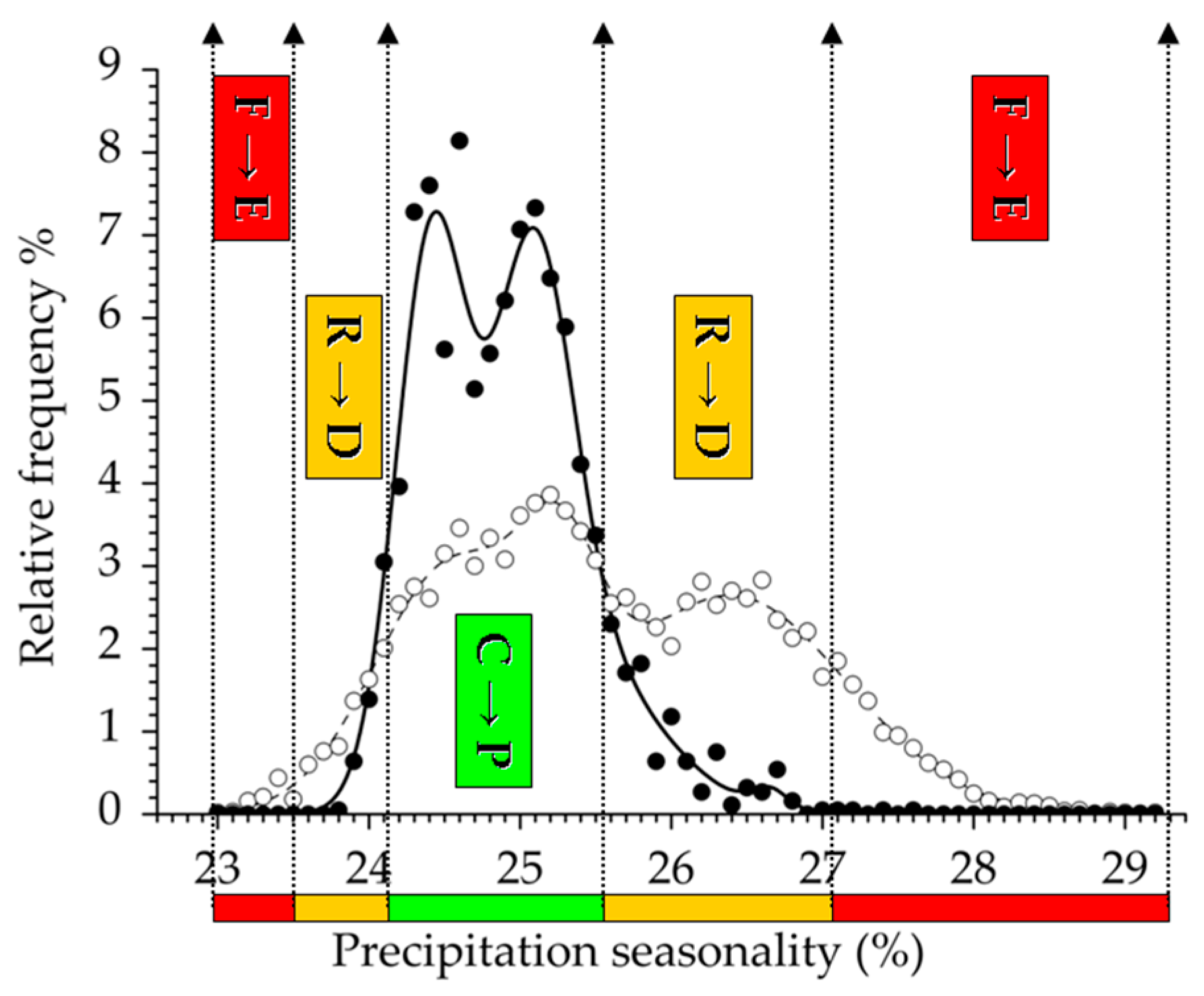
Functional climatic traits of variables extracted in the third and the fourth principal components were highly variable in their response range pattern. Continentality index (Ci) exhibited prevalence and decay functions, but the absence of the exclusion range. Isothermality (BIO3) estimates a continuous PDE trait that also contains the trailing edge of the distribution. Temperature seasonality (BIO4) indicates two decay functions, i.e., the climatic leading and the trailing edges. Finally, a totally complete functional response trait is demonstrated by Precipitation seasonality (BIO15), consisting of two separated decay and exclusion ranges that refers to the presence both of leading and trailing functional edges in the distribution.
3.3. Climatic Behavior Estimation by ROC Analysis
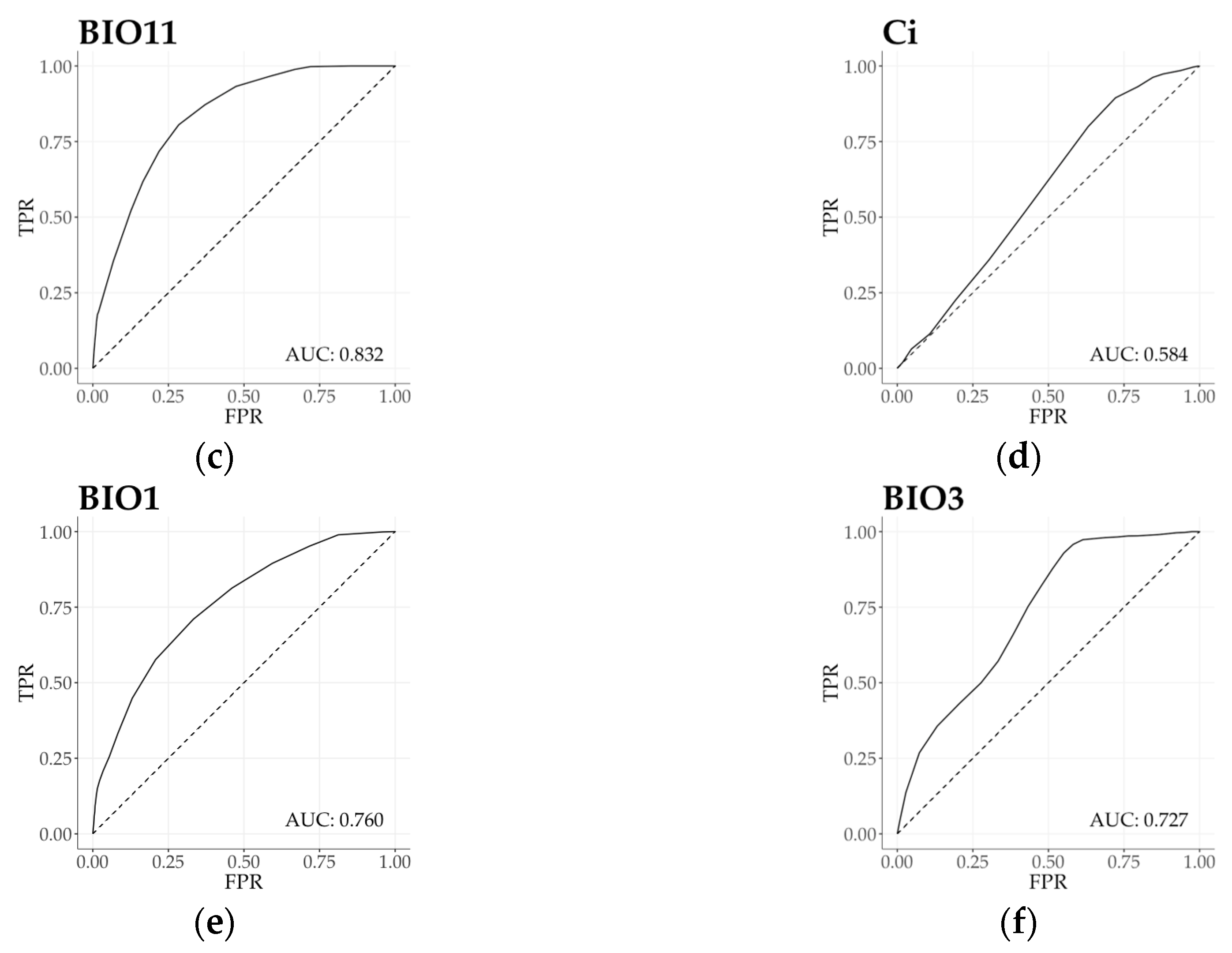
Based on the regional functional responses, we calculated ROC curves with AUC value to evaluate the overall relationship between two samples (forest as subject and region as reference), and to present the estimation power of each bioclimatic variable (Figure 4 and Figure S2). Bioclimatic variables in the first principal component provided a primary set to describe beech forest functional variability. Functional response unconformity was detected by ROC curve and AUC value of all bioclimatic variables (AUC > 0.5). Precipitation in the wettest month (BIO13) indicated the highest level of relative distinctness (AUC = 0.809), and Annual precipitation (BIO12) proved to have the lowest distinctive power (AUC = 0.755). According to temperature and related bioclimatic variables of the second principal component, all measures indicated high level of functional distinction. Minimum temperature of the coldest month (BIO6) presented the highest level of separation (AUC = 0.850). Temperature annual range (BIO7) exhibited the weakest distinction in beech forest functional distribution (AUC = 0.594), converging to be a random classifier. Moving towards climatic measures in the third and the fourth principal components, Isothermality (BIO3) and Precipitation seasonality (BIO15) indicated a moderate distinction in climate response functions. On the other hand, Continentality index (Ci; AUC = 0.584) and Temperature seasonality (BIO4; AUC = 0.543) were both occurred as nearly random classifiers.
Regarding our interpretation, distribution response functions (PDE), and derived measures (A; H), and the overall functional distribution estimator (AUC value) can all be defined as appropriate quantity to characterize sensitivity, resilience or/and adaptation. These measures together and on their own can reliably interpret the environmental limitation of the distribution as well as an intrinsic condition of the response functions.
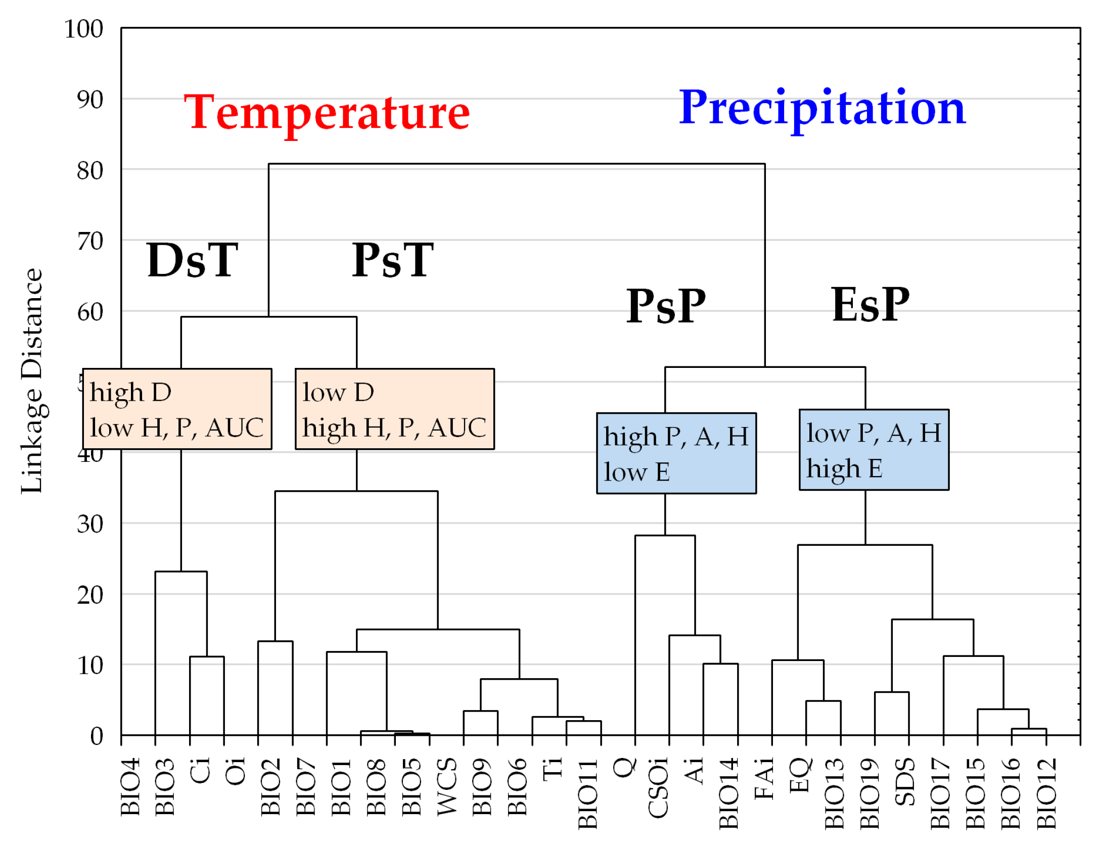
Hierarchical clustering constructed by the six aspects of beech forests response functions, two groups of bioclimatic indices are clearly discriminated, and both of them were further divided into two sub-clusters (Figure 5). The first group contains temperature-related indices corresponding to variables of the second and the third principal components of the factor analysis. The second group contains precipitation and related composite indices consisting of variables extracted in the first and fourth principal components in the factor analysis (see also Table 1). Note that the response trait of temperature indices can be generally characterized by a higher ratio of prevalence and decay functions with the exception of the exclusion range, as opposed to similar response functions of the variables in the precipitation group (see also Table 2).
Climate response functions (PDE) in the temperature group generally indicated more favorable trait patterns compared to those of the precipitation group, presenting significantly higher prevalence range (adjusted Z = −3.566, p < 0.001), amplitude (adjusted Z = −4.391, p < 0.001), and more reduced exclusion range (adjusted Z = 4.391, p < 0.001) (two-case boxplots are not presented). The temperature group introduced five bioclimatic indices even without any regional exclusion function, including Annual mean temperature (BIO1), Maximum temperature of the warmest month (BIO5), Temperature annual range (BIO7), Mean temperature of the wettest quarter (BIO8), and Continentality (Ci) (see also Table 2 and Figure 5).
Temperature and related (composite) indices in the temperature group generally resulted in more favorable climate response patterns by presenting higher amplitude and decay functions, but lower levels of exclusion function (Figure 2, Table 2; Figure S1). The temperature group was further divided into two sub-clusters according to the significant difference in decay response function (adjusted Z = 2.491; p < 0.050), and Prevalence response function (adjusted Z = −2.413; p < 0.050), Hardiness (adjusted Z = −2.491, p < 0.050), and the AUC ratio (adjusted Z = −2.335, p < 0.050) (Figure 5). The first sub-cluster was the Decay-specific Temperature group (DsT), consisting of three variables from the third component corresponding to temperature extremities. This sub-cluster can be characterized by the high ratio of decay function and lower level of prevalence range, resulting in high hardiness ratio. The second sub-cluster is the Prevalence-specific Temperature group (PsT), which consists of 11 diversified temperature indices. All of these variables indicate high levels of prevalence function but low levels of decay range. The most favorable response pattern was detected by the Annual mean temperature (BIO1), with a high prevalence ratio (76.7%) and a widely extended (up to 11.5 °C) decay range as the regional upper limit (see also Figure 4).
Precipitation and related (composite) indices in the precipitation group generally resulted in climate response patterns with lower amplitude and higher exclusion functions compared to those of the temperature group. All variables in this group presented more or less extended exclusion function than temperature trait patterns (Figure 2, Table 2; Figure S1). Cluster analysis further separated two subunits of the precipitation variables, regarding their prevalence function (adjusted Z = 2.546, p < 0.050) and exclusion function (adjusted Z = −2.546, p < 0.050), and moreover, by the amplitude (adjusted Z = 2.546, p < 0.050) and the hardiness (adjusted Z = 2.237, p < 0.050) (Figure 5). The first subunit is the Prevalence-specific Precipitation group (PsP) that can be characterized by a higher ratio of prevalence range, amplitude and hardiness, but significantly lower level of exclusion function compared to the second subunit the Exclusion Specific Precipitation group (EsP). Note, that these two subunits were not consistent with the principal components extracted in the factor analysis. PsP variables can be classified into temperature-related drought predictors: Aridity index (Ai), Compensated Summer Ombrothermic index (CSOi), Pluviothermic Quotient (Q) and Precipitation of the driest month (BIO14). The EsP subunit indicated the least favorable distributional response pattern, presenting consistently high level of exclusion function, and low levels of prevalence, amplitude, and hardiness ratio (Figure 6). The EsP group included six precipitation indices and three precipitation-related composite variables, such as Forestry Aridity index (FAi), Ellenberg’s Quotient (EQ) and Summer Drought Stress (SDS). Forestry Aridity index indicated the most unfavorable precipitation pattern with the largest exclusion response function (see Table 2).
4. Discussion
In our investigation, we studied regional climate sensitivity and resilience of Illyrian beech forests under wet continental climate conditions at a distributional trailing edge. We used 27 temperature and precipitation bioclimatic variables and related composite indices and calculated relative frequency data from presence-absence records of beech forests as the subject and the geographic area as the reference. Using these datasets, we constructed climatic response traits of beech forests, presenting complete or incomplete patterns of climate response functions. Moreover, we used basic response functions of the distribution (Prevalence, Decay and Exclusion), and three ratios derived from these (Amplitude, Hardiness and AUC) to evaluate climatic sensitivity, resilience and adaptation of beech forests. Functional response trait patterns suggested that temperature regime was a supportive element of the regional environment at a given level of precipitation. Temperature difference of the hottest and coldest months and annual mean proved to be the best predictors for beech forest adaptation and resilience. The ratio of absolute temperature difference of the hottest and the coldest months and the annual precipitation indicated the most limiting temperature-related climate regime. On the other hand, precipitation patterns turned out to be more limiting ecological functions, presenting highly extended exclusion functions, especially at the trailing distribution edges. Annual variation of precipitation indicated the highest sensitivity, presenting exclusion functions both at the leading and trailing climatic edges. Furthermore, the ratio of the precipitation sum and the mean temperature sum in the summer season was validated as the best performing rainfall predictor. Climate resilience can also be supported by high amount of precipitation during the coldest quarter (winter season).
We also performed ROC analysis to estimate the overall functional distribution performance of beech forests by using all bioclimatic variables. In case of climate-induced forests the reliability of climate modes is considered “fair” if AUC > 0.7 and “good” if AUC > 0.8 [11,21]. In our study, median AUC reached “fair” for the main groups of both clusters (AUC = 0.785 for the temperature group, and AUC = 0.768 for the precipitation group). The area ratio values of five bioclimatic variables in the temperature group were even “good” (AUC > 0.8), in contrast to the three indices in the precipitation group. Concordance of AUC values and the results of the factor and cluster analyses imply that the predictive ability of temperature-related variables is higher than that of the precipitation-related indices in this region. Temperature-related indices are frequently reported to be the best predictors of beech forest distribution in studies throughout Europe. Six predictors from the first 10 for hemi-boreal beech forests; eight important indices for sub-atlantic and sub-continental beech forests; and nine variables for Pannonian-Pontic beech forests turned out to be temperature-related climate measures [11]. Additionally, the temperature gradient was reported to involve the first division level in the TWINSPAN classification of European beech forests at a continental scale [12]. In spite of the small difference in significant environmental factors, the primary importance of temperature measures was detected at lower/southern and upper/northern climatic distribution limits of Fagus species at a global scale [16]. Note that the Thermicity index (Ti), which refers to the sum of yearly mean, maximum and minimum temperature of the coldest month, was ranked as the tenth most important predictor for sub-continental beech forest occurrence [11]. Comparing previous findings to our results, this bioclimatic measure proved to be similarly subordinate within the PAT subunit to describe functional distribution performance of beech forests. In general, projected adaptation performance of beech forests can be predicted by their long term regional existence or a small retraction by the indication of temperature variables with a high decay function ratio.
On the other hand, a warmer climate with higher temperature alone can increase forest mortality, and it can accelerate drought-induced forest decline at the global scale [62]. In our study, precipitation-related variables presented medium amplitude ratio with prevalence dominance (Table 2; Figure 6), which indicated a relatively good current state. In addition, the extremely low decay range ratio of variables in this group indicates that beech forests in southern Transdanubia can be highly threatened by drought, in accordance with previous regional results [20,29]. European beech trees and forests have also been reported to be particularly affected by summer droughts, as well as by May and July high temperatures, annual precipitation, and the temperature-to-rainfall ratio in the transitional forest-steppe vegetation zone [21]. The above-mentioned findings were similar in the Mediterranean and related regions [26]. During the growing season beech tree growth is consistently limited by high temperature and low precipitation at the southern edge of their European distribution [25,27]. Nevertheless, site-specific adaptation of the species can compensate for the unfavorable ecological or functional effects of decreasing precipitation [63], as it was also detected in the current investigation.
Previous and current studies suggest that precipitation-related bioclimatic composites are suitable as an indicator for adaptation and sensitivity at the xeric limit of distribution [19,21,23]. In our study, an extremely high level of the exclusion function was presented by Precipitation seasonality (BIO15, see Table 2), that seems to be an independent and appropriate measure for climatic sensitivity. Beech forests also present a climatic leading range by the decay function to mitigate unfavorable climate conditions and change. In summary, Precipitation seasonality proved to be the most sensitive precipitation indicator in functional response analysis. Functional response on winter season temperature (BIO19) highlights the importance of rainfall during the coldest period. The unfavorable effects of decreasing summer precipitation can also be mitigated by a flexible adaptation as it was concluded from the results of three precipitation variables referring to the hottest months of the year (SDS, BIO16 and BIO19). In our study, Ellenberg’s Quotient, the most widely used composite index in relation with climate adaptation and sensitivity (e.g., [15,16,20,22,23]), did not proved to have a powerful sensitivity indication power due to the low ratio of decay function (Table 2). This conclusion is consistent with the findings that EQ ranked 35th of 44 climatic predictors of European forest distribution [11]. In our study, composite indices did not produce a separate cluster or sub-unit, but they were classified as part of the precipitation-related group, which proved to be a more sensitive indicator of climate change, except for the Ombrothermic Index (Figure 5). Our results were in accordance with the widely accepted opinion that composite indices reflecting both ecologically important climatic variables (temperature and precipitation are better climatic predictors compared to simple (bio) climatic variables [19,54,64,65].
Precipitation indices suggested less favorable regional response patterns and adaptation. All bioclimatic variables presented a more or less expanded exclusion response range that highlights the limitation function of the current precipitation regime. Forestry Aridity index turned out to be the most important composite in adaptation estimation and xeric limit indication with the most extended exclusion function [19]. Furthermore, climatic trait performance of beech forest on Precipitation seasonality can also be used to detect and predict ecological vulnerability, potentially making this precipitation variable a highly sensitive region-specific climate indicator and a powerful estimator among functional responses.
Regarding the precipitation-related variables, favorable adaptation response pattern was detected by using Aridity index, February precipitation, Compensated Summer Ombrothermic index, and Pluviothermic Quotient. The last two temperature-induced precipitation bioclimatic variables indicate that we have to be cautious when discussing functional processes under climate change and adaptation assessment. Winter season precipitation (i.e., the coldest quarter of the year) will also be an important factor for ecological resilience during climate change adaptation. Setting up a regional environmental monitoring system that measures local precipitation is necessary to establish and implement a regional adaptive forest management [66].
5. Conclusions
Temperature response patterns indicated a more favorable state of resilience and adaptation than precipitation indices. Regarding the high resolution and region-specific forecasted trends of climate change by moderately increasing mean temperature and constantly fluctuating sum of precipitation [67], and our results of climate response patterns, only a minor shifting in beech forests distribution could be predicted in the near future. Precipitation-related climate sensitivity predictors, especially the Precipitation seasonality and the Forestry Aridity index could be the most sensitive rainfall indicators. The most favorable temperature response variables, such as Continentality can refer to the highest level of resilience in spite of increasing temperature regimes.
Communicating scientific results towards decision makers in forestry is an ongoing challenge, especially when these results are burdened with uncertainties, as it is the case of climate change and its impacts on forests [68]. Large-scale studies do not necessarily provide suitable information for local forest planning and management strategies. Furthermore, the precipitation scenario predictions for the Mediterranean and nearby regions including our study area [68] carry a high level of uncertainty. Consequently, the role of climate extremities is very important and precipitation seasonality in particular could be the most powerful rainfall response estimator. Among the three alternative forest management strategies proposed for Central Europe, the conservation of existing forest structures seems to be a better option than active or passive adaptive management [66]. This strategy is more compatible with the principles of close-to-nature forestry [69], which is increasingly applied in beech forests throughout Hungary. Under this framework, five principles can be implemented for enhancing the adaptive capacity of forests in response to climate change: increase species structural and genetic diversity; increase resistance of individual trees to biotic and abiotic stress and keep growing stock low [70].
Supplementary Materials
The following are available online at www.mdpi.com/1999-4907/8/9/324/s1, Table S1: Bioclimatic frequency data for beech forests and the geographic region; Figure S1: Climatic response traits of beech forests based on 21 bioclimatic variables; Figure S2: ROC curves and AUC values of beech forests based on 21 bioclimatic variables.
Acknowledgments
Field data collection was financed by MÉTA habitat framework project NKFP 3B/0050 (Széchenyi Plan 2004–2007). Thanks to MÉTA Advisory Board and MÉTA Informatics for providing forest and climate datasets. Special thanks to Bálint Czúcz (HAS IEB) for downscaling the climatic data to hexagon scale. The authors are grateful to two anonymous rewievers for their suggestions and the improvement of the manuscript. The Faculty of Sciences at the University of Pécs covered the cost to publish this article as open access by fund EFOP 3.6.1-16-2016-00004 Comprehensive Development for Implementing Smart Specialization Strategies at the University of Pécs. This project has been supportedby the Euprpean Union, co-financed bu the European Social Fund. This scientific contribution is dedicated to the 650th anniversary of the foundation of the University of Pécs, Hungary.
Author Contributions
É.S.-A. and A.O.-A. conceived and designed the analyses and developed the theoretical background, É.S.-A. and G.A. performed statistical analyses, É.S.-A. and A.O.-A. contributed to field data collection, and all the co-authors contributed to writing the main text and the revision of the manuscript.
Conflicts of Interest
The authors declare no conflict of interest. The funding sponsors had no influence on the design, analyses, data interpretation, writing of the manuscript, and the decision to publish the results.
References
- Violle, C.; Navas, M.L.; Vile, D.; Kazakou, E.; Fortunel, C.; Hummel, I.; Garnir, E. Let the concept of trait be functional! Oikos 2007, 116, 882–892. [Google Scholar] [CrossRef]
- Díaz, S.; Purvis, A.; Cornelissen, J.H.C.; Mace, M.G.; Donoghue, M.J.; Ewers, R.M.; Jordano, P.; Pearse, W.D. Functional traits, the phylogeny of function, and ecosystem service vulnerability. Ecol. Evol. 2013, 3, 2958–2975. [Google Scholar] [CrossRef] [PubMed]
- Nock, C.A.; Vogt, R.J.; Beisner, B.E. Functional Traits. eLS 2016, 1–8. [Google Scholar] [CrossRef]
- Walther, G.-R. Community and ecosystem responses to recent climate change. Phil. Trans. R. Soc. B 2010, 365, 2019–2024. [Google Scholar] [CrossRef] [PubMed]
- Cadotte, M.W.; Carscadden, K.; Mirotchnick, N. Beyond species: Functional diversity and the maintenance of ecological processes and services. J. Appl. Ecol. 2011, 48, 1079–1087. [Google Scholar] [CrossRef]
- Grimm, N.B.; Chapin, F.S.; Bierwagen, B.; Gonzalez, P.; Groffman, P.M.; Luo, Y.; Melton, F.; Nadelhoffer, K.; Pairis, A.; Raymond, P.A.; et al. The impacts of climate change on ecosystem structure and function. Front. Ecol. Environ. 2013, 11, 474–482. [Google Scholar] [CrossRef]
- Adger, W.N.; Agrawala, S.; Mirza, M.M.Q.; Conde, C.; O’Brien, K.; Pulhin, J.; Pulwarty, R.; Smit, B.; Takahashi, K. Assessment of adaptation practices, options, constraints and capacity. In Climate Change 2007: Impacts, Adaptation and Vulnerability. Contribution of Working Group II to the Fourth Assessment Report of the Intergovernmental Panel on Climate Change; Parry, M.L., Canziani, O.F., Palutikof, J.P., van der Linden, P.J., Hanson, C.E., Eds.; Cambridge University Press: Cambridge, UK, 2007; pp. 717–743. [Google Scholar]
- Kolström, M.; Lindner, M.; Vilén, T.; Maroschek, M.; Seidl, R.; Lexer, M.; Netherer, S.; Kremer, A.; Delzon, S.; Barbati, A.; et al. Reviewing the Science and Implementation of Climate Change Adaptation Measures in European Forestry. Forests 2011, 2, 961–982. [Google Scholar] [CrossRef] [Green Version]
- Adaptation and Mitigation. Available online: http://know.climateofconcern.org/index.php?option=com_content&task=article&id=139 (accessed on 14 July 2017).
- Climate Change Synthesis Report: Annex B 2001. Available online: https://gridarendal-website.s3.amazonaws.com/production/documents/:s_document/293/original/annex.pdf?1488203667 (accessed on 23 August 2017).
- Casalegno, S.; Amatulli, G.; Bastrup-Birk, A.; Houston Durrant, T.; Pekkarinen, A. Modelling and mapping the suitability of European forest formations at 1-km resolution. Eur. J. For. Res. 2011, 130, 971–981. [Google Scholar] [CrossRef]
- Willner, W.; Jimenez-Alfaro, B.; Agrillo, E.; Biurrun, I.; Campos, J.A.; Carni, A.; Casella, L.; Csiky, J.; Custerevska, R.; Didukh, J.P.; et al. Classification of European beech forests: A Gordian knot ? Appl. Veg. Sci. 2017, 20, 494–512. [Google Scholar] [CrossRef]
- Ozenda, P.; Borel, J.L. An ecological map of Europe: Why and how? C. R. Acad. Sci. 2000, 983–994. [Google Scholar] [CrossRef]
- Dengler, A. Waldbau auf Ökologischer Grundlage, 3rd ed.; Springer: Berlin, Germany, 1944. [Google Scholar]
- Bolte, A.; Czajkowski, T.; Kompa, T. The north-eastern distribution range of European beech—A review. Forestry 2007, 80, 413–429. [Google Scholar] [CrossRef]
- Fang, J.; Lechowicz, M.J. Climatic limits for the present distribution of beech (Fagus L.) species in the world. J. Biogeogr. 2006, 33, 1804–1819. [Google Scholar] [CrossRef]
- Augustaitis, A.; Kliučius, A.; Marozas, V.; Pilkauskas, M.; Augustaitiene, I.; Vitas, A.; Staszewski, T.; Jansons, A.; Dreimanis, A. Sensitivity of European beech trees to unfavorable environmental factors on the edge and outside of their distribution range in north-eastern Europe. iForest 2015, 9, 259–269. [Google Scholar] [CrossRef]
- Marinšek, A.; Šilc, U.; Čarni, A. Geographical and ecological differentiation of Fagus forest vegetation in SE Europe. Appl. Veg. Sci. 2013, 131–147. [Google Scholar] [CrossRef]
- Salamon-Albert, É.; Lőrincz, P.; Pauler, G.; Bartha, D.; Horváth, F. Drought stress distribution responses of continental beech forests at their xeric edge in Central Europe. Forests 2016, 7, 298. [Google Scholar] [CrossRef]
- Mátyás, C.; Berki, I.; Czúcz, B.; Gálos, B.; Móricz, N.; Rasztovits, E. Future of beech in Southeast Europe from the perspective of evolutionary ecology. Acta Silv. Lign. Hung. 2010, 6, 91–110. [Google Scholar]
- Czúcz, B.; Gálhidy, L.; Mátyás, C. Present and forecasted xeric climatic limits of beech and sessile oak distribution at low altitudes in Central Europe. Ann. For. Sci. 2011, 68, 99–108. [Google Scholar] [CrossRef]
- Stojanović, D.B.; Kržič, A.; Matović, A.; Orlović, S.; Duputie, A.; Djurdjević, A.; Galić, A.; Stojnić, S. Prediction of the European beech (Fagus sylvatica L.) xeric limit using a regional climate model: An example from southeast Europe. Agric. For. Met. 2013, 176, 94–103. [Google Scholar] [CrossRef]
- Budeanu, M.; Petritan, A.M.; Popescu, F.; Vasile, D.; Tudose, C. The resistance of European beech (Fagus sylvatica) from the eastern natural limit of species to climate change. Not. Bot. Horti Agrobot. 2016, 44, 625–633. [Google Scholar] [CrossRef]
- Gálos, B.; Führer, E.; Czimber, K.; Gulyás, K.; Bidló, A.; Hänsler, A.; Jacob, D.; Mátyás, C. Climatic threats determining future adaptive forest management—A case study of Zala County. Időjárás 2015, 119, 425–441. [Google Scholar]
- Hacket-Pain, A.J.; Cavin, L.; Friend, A.D.; Jump, A.S. Consistent limitation of growth by high temperature and low precipitation from range core to southern edge of European beech indicates widespread vulnerability to changing climate. Eur. J. For. Res. 2016. [Google Scholar] [CrossRef]
- Di Filippo, A.; Biondi, F.; Čufar, K.; De Luis, M.; Grabner, M.; Maugeri, M.; Saba, E.P.; Schirone, B.; Piovesan, G. Bioclimatology of beech (Fagus sylvatica L.) in the Eastern Alps: Spatial and altitudinal climatic signals identified through a tree-ring network. J. Biogeogr. 2007, 1873–1892. [Google Scholar] [CrossRef]
- Tegel, W.; Seim, A.; Hakelberg, D.; Hoffmann, S.; Panev, M.; Westphal, T.; Büntgen, U. A recent growth increase of European beech (Fagus sylvatica L.) at its Mediterranean distribution limit contradicts drought stress. Eur. J. For. Res. 2014, 133, 61–71. [Google Scholar] [CrossRef]
- Michelot, A.; Bréda, N.; Damesin, C.; Dufrêne, E. Differing growth responses to climatic variations and soil water deficits of Fagus sylvatica, Quercus petraea and Pinus sylvestris in a temperate forest. For. Ecol. Manag. 2012, 265, 161–171. [Google Scholar] [CrossRef]
- Lindner, M.; Maroschek, M.; Netherer, S.; Kremer, A.; Barbati, A.; Garcia-Gonzalo, J.; Seidl, R.; Delzon, S.; Corona, P.; Kolström, M.; et al. Climate change impacts, adaptive capacity, and vulnerability of European forest ecosystems. For. Ecol. Manag. 2010, 259, 698–709. [Google Scholar] [CrossRef]
- Bolte, A.; Czajkowski, T.; Cocozza, C.; Tognetti, R.; de Miguel, M.; Psidova, E.; Ditmarova, L.; Dinca, L.; Delzon, S.; Cochard, H.; et al. Desiccation and Mortality Dynamics in Seedlings of Different European Beech (Fagus sylvatica L.) populations under Extreme Drought Conditions. Front. Plant Sci. 2016, 7, 1–12. [Google Scholar] [CrossRef] [PubMed]
- Nahm, M.; Radoglou, K.; Halyvopoulos, G.; Gessler, A.; Renneberg, H.; Fotelli, M.N. Physiological Performance of Beech (Fagus sylvatica L.) at its Southeastern Distribution Limit in Europe: Seasonal Changes in Nitrogen, Carbon and Water Balance. Plant Biol. 2006, 8, 52–63. [Google Scholar] [CrossRef] [PubMed]
- Fotelli, M.N.; Nahm, M.; Radoglu, K.; Renneberg, H.; Halyvopulus, G.; Matzarakis, A. Seasonal and interannual ecophysiological responses of beech (Fagus sylvatica) at its south-eastern distribution limit in Europe. For. Ecol. Manag. 2009, 257, 1157–1164. [Google Scholar] [CrossRef]
- De Candolle, A. Origin of Cultivated Plants; Appleton: New York, NY, USA, 1855; p. 497. [Google Scholar]
- Köppen, F.T. Geographische Verbreitung der Holzgewächse des Europäischen Russlands und des Kaukasus; Kaiserlichen Akademie der Wissenschaften: St. Petersburg, Russia, 1889. [Google Scholar]
- Europe’s Biodiversity—Biogeographical Regions and Seas. Biogeographical Regions in Europe. The Pannonian Region. Available online: https://www.eea.europa.eu/publications/report_2002_0524_154909 (accessed on 13 July 2017).
- Mersich, I.; Práger, T.; Ambrózy, P.; Hunkár, M.; Dunkel, Z. Climate Atlas of Hungary (in Hungarian); Hungarian Meteorological Service: Budapest, Hungary, 2001; p. 107. [Google Scholar]
- Climate of Hungary—General Characteristics. Available online: http://www.met.hu/en/eghajlat/magyarorszag_eghajlata/altalanos_eghajlati_jellemzes/altalanos_leiras/ (accessed on 14 July 2017).
- Peel, M.C.; Finlayson, B.L.; McMahon, T.A. Updated world map of the Köppen-Geiger climate classification. Hydrol. Earth Syst. Sci. 2007, 11, 1633–1644. [Google Scholar] [CrossRef]
- Borhidi, A. Klimadiagramme und klimazonale Karte Ungarns. Ann. Univ. Sci. Budapest. Sec. Geogr. 1961, 4, 21–50. [Google Scholar]
- Zólyomi, B.; Kéri, M.; Horváth, F. Spatial and temporal changes in the frequency of climatic year types in the Carpathian Basin. Coenoses 1997, 12, 33–41. [Google Scholar]
- Distribution Map of Fagus sylvatica. Available online: http://www.euforgen.org/species/fagus-sylvatica/ (accessed on 7 October 2017).
- MÉTA—Methodology. Available online: http://www.novenyzetiterkep.hu/english/node/59 (accessed on 14 July 2017).
- Molnár, Z.; Bartha, S.; Seregélyes, T.; Illyés, E.; Botta-Dukát, Z.; Tímár, G.; Horváth, F.; Révész, A.; Kun, A.; Bölöni, J.; et al. A grid-based, satellite-image supported, multi-attributed vegetation mapping method (MÉTA). Folia Geobot. 2007, 42, 225–247. [Google Scholar] [CrossRef]
- EEA. European Forest Types—Categories and Types for Sustainable Forest Management Reporting and Policy. 2006. Available online: https://www.eea.europa.eu/publications/technical_report_2006_9 (accessed on 13 July 2017).
- Bölöni, J.; Molnár, Z.; Biró, M.; Horváth, F. Distribution of the (semi-)natural habitats in Hungary II. Woodlands and shrublands. Acta Bot. Hung. 2008, 50, 107–148. [Google Scholar] [CrossRef]
- Borhidi, A.; Kevey, B.; Lendvai, G. Plant Communities of Hungary, 1st ed.; Akadémiai Kiadó: Budapest, Hungary, 2012; pp. 423–426. [Google Scholar]
- Csiky, J.; Borhidi, A.; Bölöni, J.; Fekete, G.; Nagy, J.; Tímár, G.; Ódor, P.; Bartha, D.; Bodonczi, L. K5—Beech forests. In Magyarország élőhelyei; Vegetációtípusok leírása és határozója—ÁNÉR 2011 (in Hungarian); Bölöni, J., Molnár, Z., Kun, A., Eds.; MTA Ökológiai és Botanikai Kutatóintézet: Vácrátót, Hungary, 2011; pp. 268–273. [Google Scholar]
- Hijmans, R.J.; Cameron, S.E.; Parra, J.L.; Jones, P.G.; Jarvis, A. Very high resolution interpolated climate surfaces for global land areas. Int. J. Clim. 2005, 25, 1965–1978. [Google Scholar] [CrossRef]
- Bioclim—Bioclimatic variables. Available online: http://www.worldclim.org/bioclim (accessed on 14 July 2017).
- Bihari, Z. Climate Atlas of Hungary (in Hungarian). In Forest and Climate (in Hungarian); Mátyás, C., Víg, P., Eds.; University of West Hungary: Sopron, Hungary, 2004; pp. 23–34. [Google Scholar]
- Benichou, P.; Le Breton, O. Prise en compte de la topographie pour la cartographie de champs pluviométriques: la méthode AURELHY. Agrométéorol. Rég. Moy. Mont. 1986, 39, 51–69. [Google Scholar]
- De Martonne, E. Regions of interior basin drainage. Geogr. Rev. 1927, 17, 397–414. [Google Scholar] [CrossRef]
- Rivas-Martínez, S.; Sánchez-Mata, D.; Costa, M. North American boreal and western temperate forest vegetation. Itin. Geobot. 1999, 12, 5–316. [Google Scholar]
- Ellenberg, H. Vegetation Mitteleuropas mit den Alpen, 5th ed.; Ulmer: Stuttgart, Germany, 1996; p. 1095. [Google Scholar]
- Führer, E.; Horváth, L.; Jagodics, A.; Machon, A.; Szabados, I. Application of a new aridity index in Hungarian forestry practice. Idojaras 2011, 115, 205–216. [Google Scholar]
- Emberger, L. La végétation de la region méditérranéenne. Essai d’une classification des groupements végétaux. Rev. Bot. 1930, 503, 642–662. [Google Scholar]
- Mitrakos, K. A theory for Mediterranean plant life. Acta Oecol. 1980, 1, 245–252. [Google Scholar]
- Krzanowski, W.J.; Hand, D.J. ROC Curves for Continuous Data; Chapman & Hall/CRC: Boca Raton, UK, 2009. [Google Scholar]
- Origin. Available online: http://www.originlab.com/index.aspx?go=PRODUCTS/Origin (accessed on 14 July 2017).
- Statistica 12—Product Features. Available online: http://www.statsoft.com/Products/STATISTICA-Features/Version-12 (accessed on 14 July 2017).
- The R Project for Statistical Computing. Available online: https://www.r-project.org/ (accessed on 10 July 2017).
- Allen, C.D.; Macalady, A.K.; Chenchouni, H.; Bachelet, D.; McDowell, N.; Vennetier, M.; Kitzberger, T.; Rigling, A.; Breshears, D.; Hogg, E.H.T.; et al. A global overview of drought and heat-induced mortality reveals emerging climate change risks for forests. For. Ecol. Manag. 2010, 259, 660–684. [Google Scholar] [CrossRef]
- Bauwe, A.; Jurasinski, G.; Scharnweber, T.; Schröder, C.; Lennartz, B. Impact of climate change on tree-ring growth of Scots pine, common beech and pedunculate oak in northeastern Germany. iForest 2015, 9, 1–11. [Google Scholar] [CrossRef]
- Prentice, I.C.; Cramer, W.; Harrison, S.; Leemnas, R.; Monserud, A.M.; Solomon, A.M. Special Paper: A Global Biome Model Based on Plant Physiology and Dominance, Soil Properties and Climate. J. Biogeogr. 1992, 19, 117–134. [Google Scholar] [CrossRef]
- Bakkenes, M.; Alkemade, J.R.M.; Ihle, F.; Leemans, R.; Latour, J.B. Assessing effects of forecasted climate change on the diversity and distribution of European higher plants for 2050. Glob. Chang. Biol. 2002, 8, 390–407. [Google Scholar] [CrossRef]
- Bolte, A.; Ammer, C.; Löf, M.; Madsen, P.; Nabuurs, G.-J.; Schall, P.; Spathelf, P.; Rock, J. Adaptive forest management in central Europe: Climate change impacts, strategies and integrative concept. Scand. J. For. Res. 2009, 24, 473–482. [Google Scholar] [CrossRef]
- Mezősi, G.; Meyer, B.C.; Loibl, W.; Aubrecht, C.; Csorba, P.; Bata, T. Assessment of regional climate change impacts on Hungarian landscapes. Reg. Environ. Chang. 2013, 13, 797–811. [Google Scholar] [CrossRef]
- Lindner, M.; Fitzgerald, J.B.; Zimmermann, N.E.; Reyer, C.; Delzon, S.; van der Maaten, E.; Schelhaas, M.J.; Lasch, P.; Eggers, J.; ven der Maaten-Theunissen, M.; et al. Climate change and European forests: What do we know, what are the uncertainities, and what are the implications for forest management? J. Environ. Manag. 2014, 146, 68–83. [Google Scholar] [CrossRef] [PubMed]
- Pommering, A.; Murphy, S.T. A review of the history, definitions and methods of continuous cover forestry with special attention to afforestation and restocking. Forestry 2004, 77, 27–44. [Google Scholar] [CrossRef]
- Brang, P.; Spathelf, P.; Larsen, B.J.; Bauhus, J.; Boncina, A.; Chauvin, C.; Drössler, L.; Garcia-Güemes, C.; Heiri, C.; Kerr, G.; et al. Suitability of close-to-nature silviculture for adapting temperate European forests to climate change. Forestry 2014, 87, 492–503. [Google Scholar] [CrossRef]
Figure 1.
Location and characteristics of the study area. (a) Continental-scale distribution of European beech (in blue) [41]; (b) Geographic surface of the study area with the main rivers and the Lake Balaton (inland watercourses are not illustrated), and the distribution pattern of beech forests (filled circles); altitudinal zones are indicted by grey shading using the ranges in the upper left corner, southern Transdanubia in Hungary (HU). Some of neighbor countries are also indicated: Ukraine (UA), Romania (RO) and Austria (AT).
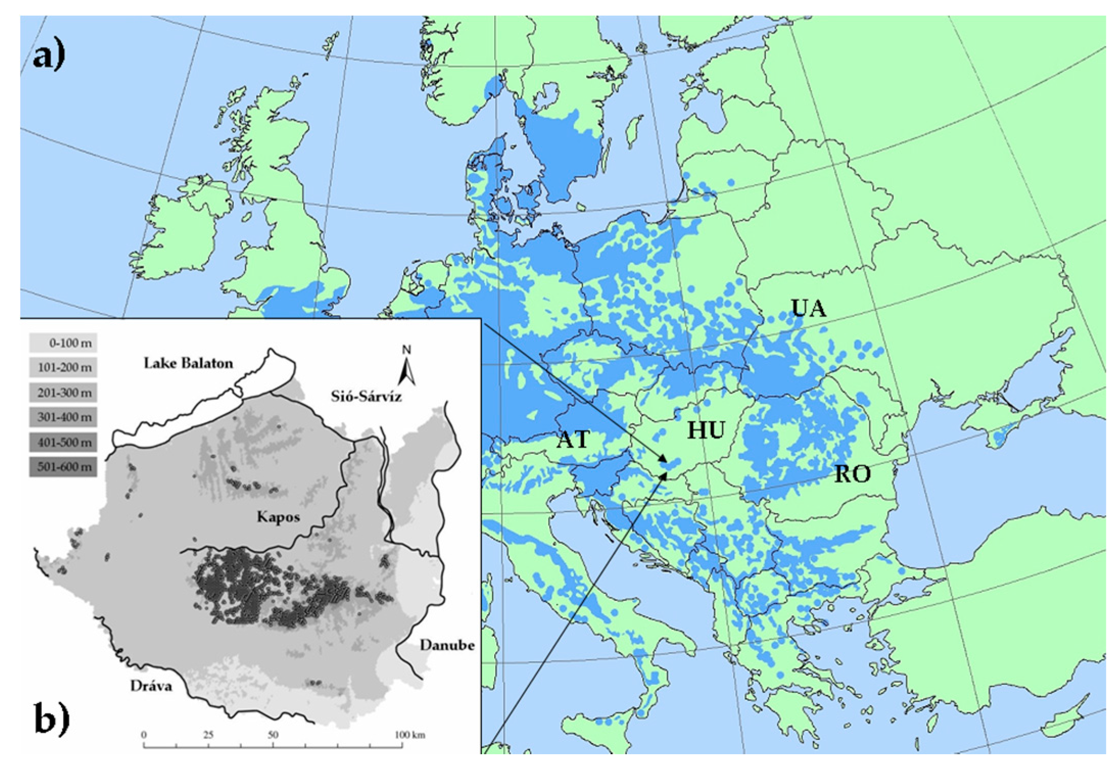
Figure 2.
Prevalence–Decay-Exclusion (PDE) response functions derived from Coping–Resilience-Failure (CRF) climatic trait ranges of beech forests (e.g., Precipitation seasonality as an example). Coping range refers to Prevalence response function (C→P; green bar); Resilience range shows the Decay response function (R→D; orange bars); and Failure range identifies the Exclusion response function (F→E; red bars). Filled dots and solid line indicate relative frequency and functional response curve of beech forests, respectively, while empty dots and dashed line refer to those of the geographic area (climatic surface). CRF ranges are calculated from the disparity of functional response curves of the region and beech forests (e.g., coping range is defined if beech forests relative frequency is higher than that of the region).

Figure 3.
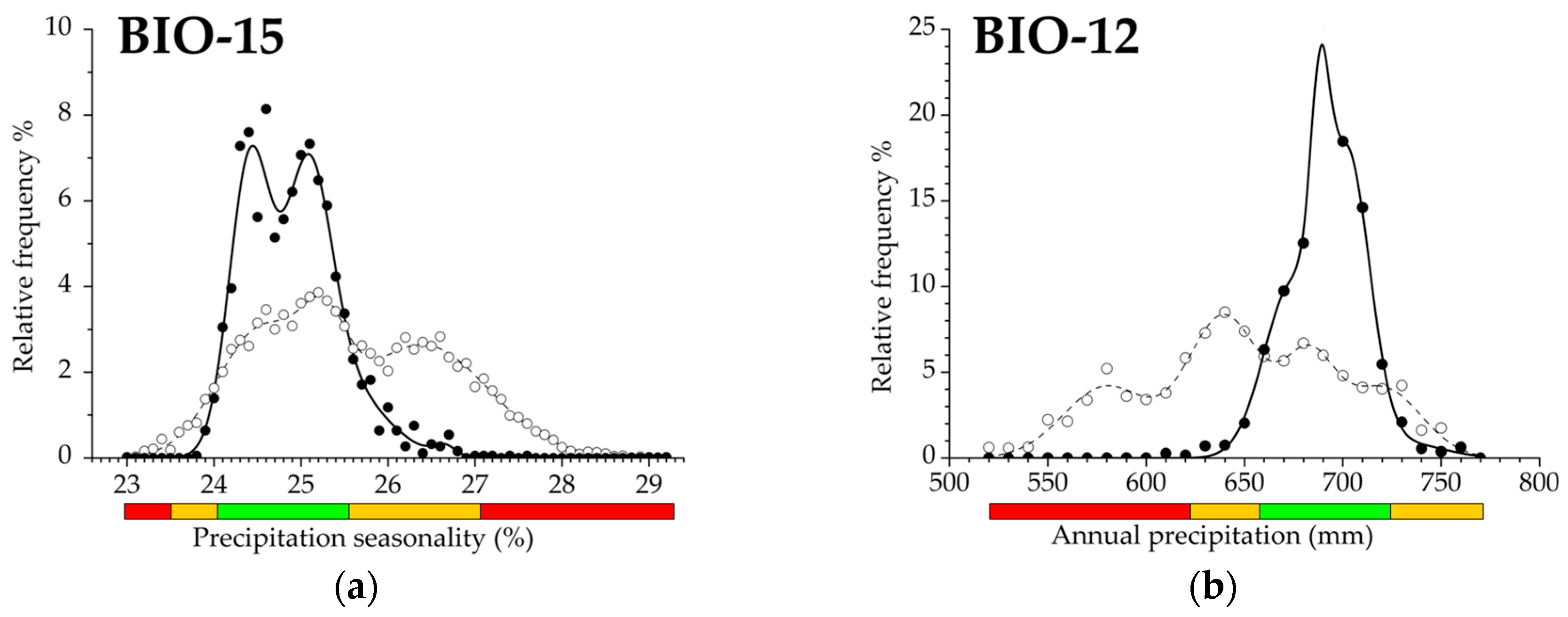
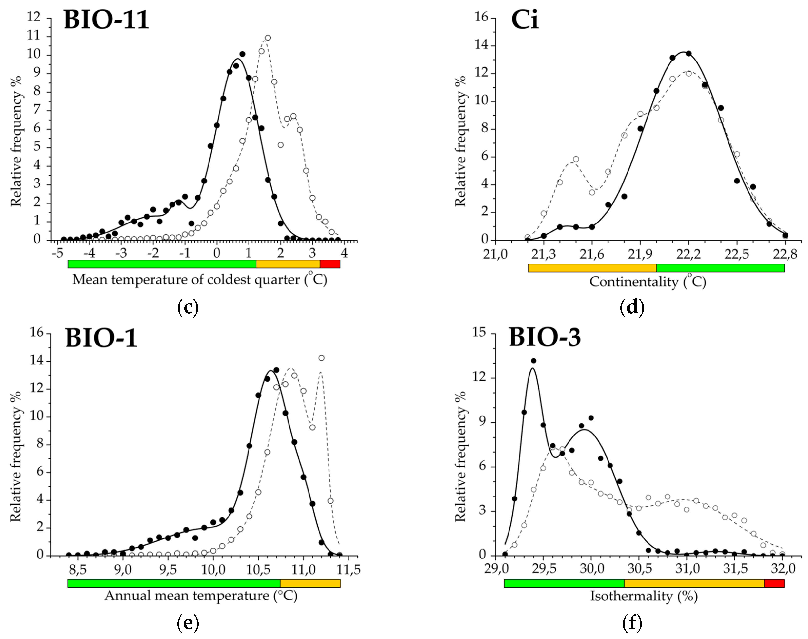
(a–f) Climatic response functions of beech forests for selected variables presenting different climatic trait patterns and modality, which differ in the number and position of decay (D) and exclusion (E) ranges (prevalence range is a regular element). (a) Response pattern with double decay and exclusion; (b) response pattern with double decay; (c) response pattern with complete but single response functions; (d) response pattern with single decay; (e) response pattern with single decay and dominant prevalence function; (f) response pattern with single and dominant decay function. Green bar: prevalence function; orange bar: decay function; red bar: exclusion function of the distribution. Filled dots and solid line illustrate relative frequency and fitted curve of beech forests (object), respectively, empty dots and dashed line sign relative frequency and functional curve for the geographic region (reference), respectively. For the dimensions of the functional response ranges see Table 2. Climatic response traits for additional variables are shown in Figure S1.
Figure 3.
(a–f) Climatic response functions of beech forests for selected variables presenting different climatic trait patterns and modality, which differ in the number and position of decay (D) and exclusion (E) ranges (prevalence range is a regular element). (a) Response pattern with double decay and exclusion; (b) response pattern with double decay; (c) response pattern with complete but single response functions; (d) response pattern with single decay; (e) response pattern with single decay and dominant prevalence function; (f) response pattern with single and dominant decay function. Green bar: prevalence function; orange bar: decay function; red bar: exclusion function of the distribution. Filled dots and solid line illustrate relative frequency and fitted curve of beech forests (object), respectively, empty dots and dashed line sign relative frequency and functional curve for the geographic region (reference), respectively. For the dimensions of the functional response ranges see Table 2. Climatic response traits for additional variables are shown in Figure S1.


Figure 4.
(a–f) ROC curves with AUC estimation (Receiving Operating Characteristic curve with Area Under the Curve) of beech forests for selected variables corresponding with climatic traits in Figure 3. (a) Precipitation seasonality (BIO15); (b) Annual precipitation (BIO12); (c) Mean temperature of the coldest quarter (BIO11); (d) Continentality (Ci); (e) Annual mean temperature (BIO1); (f) Isothermality (BIO3). Solid line indicates beech forests function and dashed line indicates random area value of the geographic region as the reference (AUC = 0.5). FRP = False Positive Rate, TRP = True Positive Rate. For ROC curves and AUC values of additional variables see Figure S2.
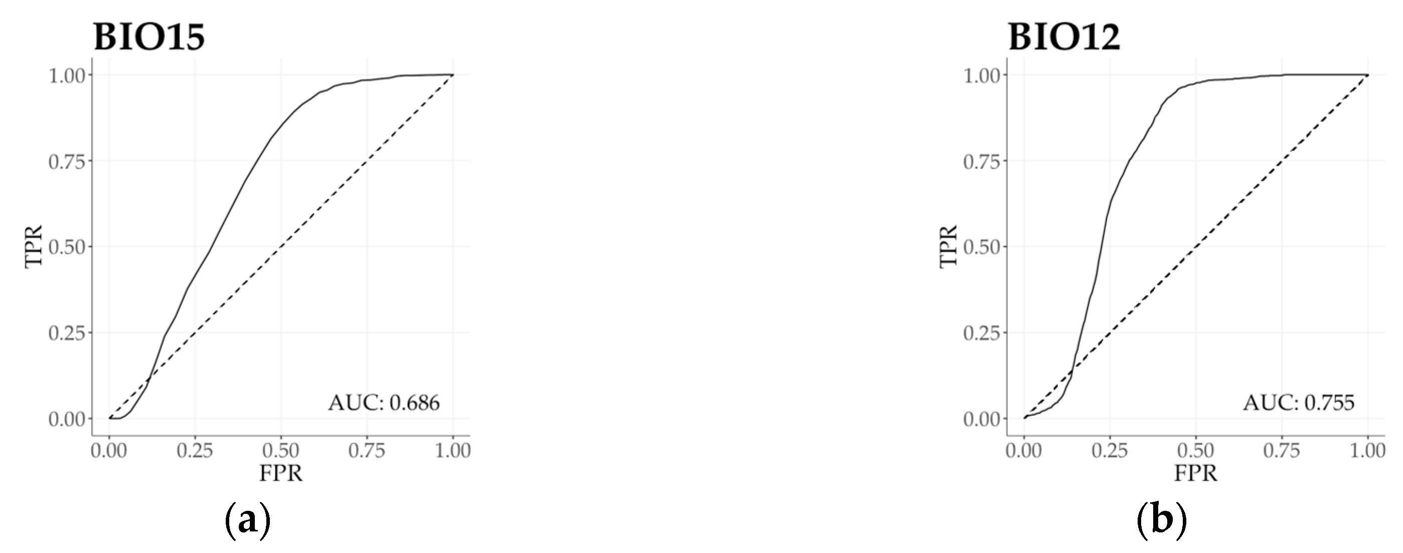

Figure 5.
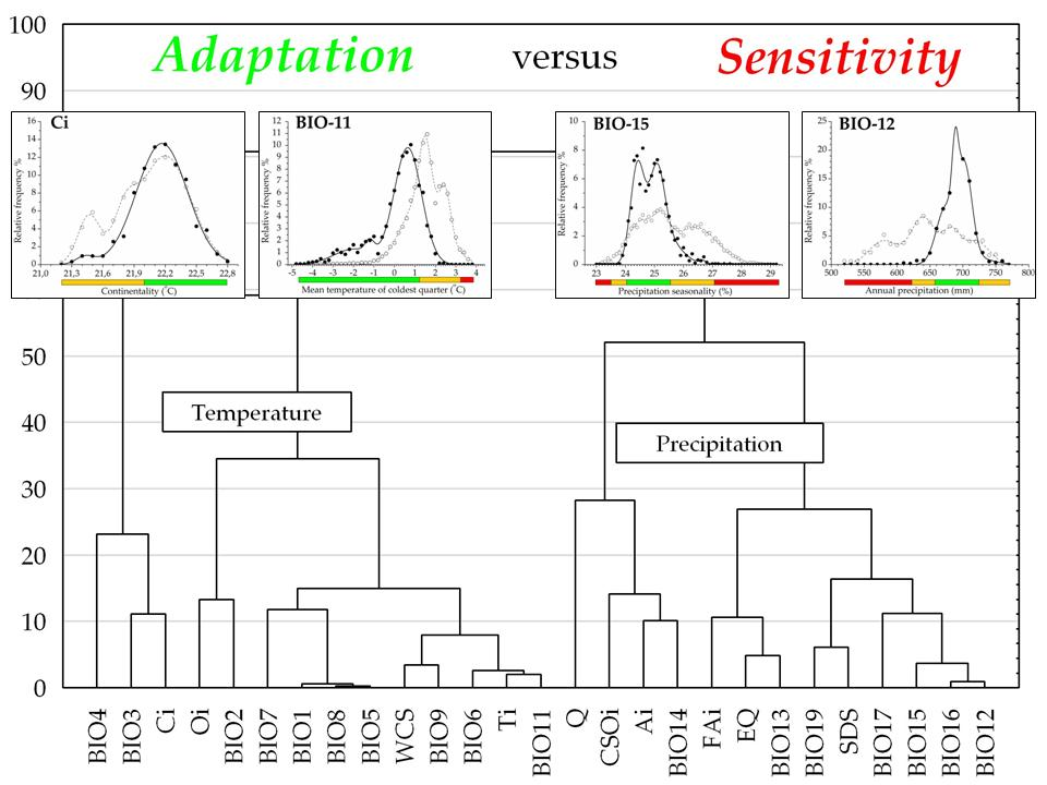
Tree diagram constructed on six response function measures on 27 bioclimatic variables (Euclidean distance, complete linkage). DsT = Decay-specific Temperature group; PsT = Prevalence-specific Temperature group; PsP = Prevalence-specific Precipitation group; EsP = Exclusion-specific Precipitation group. Name of the groups corresponds to the most important adaptation measure performing in their differentiation (Mann-Whitney U-test; p < 0.05; results are not presented). For detailed explanation of response function measures (P; D; E; A; H; AUC) and the description of bioclimatic variables (from BIO4 to BIO12) see Table 2 and Section 2.4.
Figure 5.
Tree diagram constructed on six response function measures on 27 bioclimatic variables (Euclidean distance, complete linkage). DsT = Decay-specific Temperature group; PsT = Prevalence-specific Temperature group; PsP = Prevalence-specific Precipitation group; EsP = Exclusion-specific Precipitation group. Name of the groups corresponds to the most important adaptation measure performing in their differentiation (Mann-Whitney U-test; p < 0.05; results are not presented). For detailed explanation of response function measures (P; D; E; A; H; AUC) and the description of bioclimatic variables (from BIO4 to BIO12) see Table 2 and Section 2.4.

Figure 6.
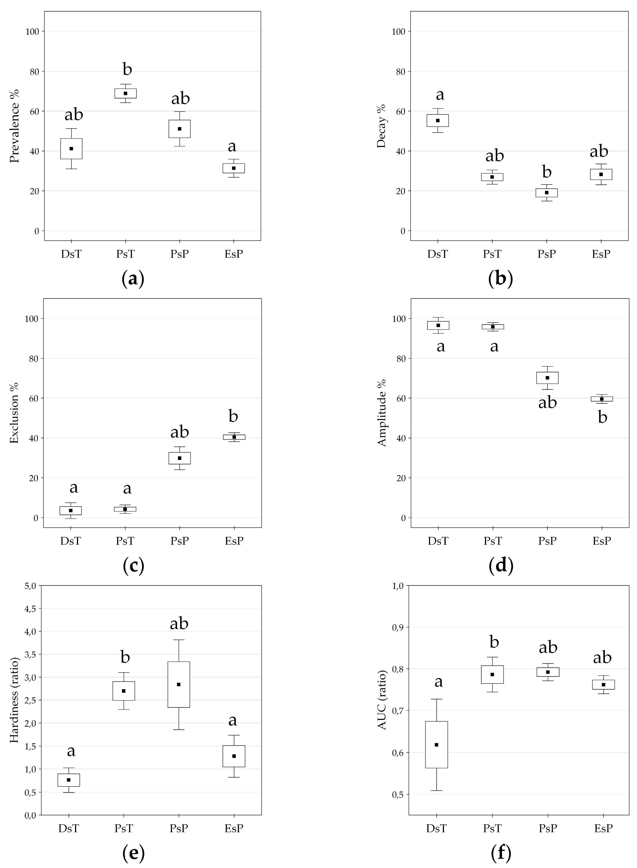
(a–f) Differences in temperature and precipitation-related functional units classified by the six response function measures of appropriate sets of variables (see also Figure 5). (a) Prevalence function; (b) Decay function; (c) Exclusion function; (d) Amplitude; (e) Hardiness; (f) Area Under the Curve (AUC value). DsT = Decay-specific Temperature group; PsT = Prevalence-specific Temperature group; PsP = Prevalence-specific Precipitation group; EsP = Exclusion-specific Precipitation group. Kruskal-Wallis test, Mean ± SE in the boxplots, significant differences are indicated by lowercase letters, p < 0.05.
Figure 6.
(a–f) Differences in temperature and precipitation-related functional units classified by the six response function measures of appropriate sets of variables (see also Figure 5). (a) Prevalence function; (b) Decay function; (c) Exclusion function; (d) Amplitude; (e) Hardiness; (f) Area Under the Curve (AUC value). DsT = Decay-specific Temperature group; PsT = Prevalence-specific Temperature group; PsP = Prevalence-specific Precipitation group; EsP = Exclusion-specific Precipitation group. Kruskal-Wallis test, Mean ± SE in the boxplots, significant differences are indicated by lowercase letters, p < 0.05.

Table 1.
Results of the exploratory factor analysis including 27 bioclimatic variables in relation to beech forests presence. Variables are listed in ascending order of principal components (PC-1; PC-2; PC-3; PC-4), and descending order of factor loadings (numbers) within a component. Abbreviation and type of variables are also indicated (P = precipitation, T = temperature, P/T or T/P = ratio).
| Variable | Abbreviation | Type | PC-1 | PC-2 | PC-3 | PC-4 |
|---|---|---|---|---|---|---|
| Annual precipitation | BIO12 | P | −0.948 | |||
| Precipitation of the wettest month 1 | BIO13 | P | −0.907 | |||
| Precipitation of the wettest/warmest quarter 2 | BIO16/BIO18 | P | −0.902 | |||
| Precipitation of the driest quarter 3 | BIO17 | P | −0.901 | |||
| Summer Drought Stress | SDS | P | 0.901 | |||
| Precipitation of the coldest quarter 4 | BIO19 | P | −0.853 | |||
| Precipitation of the driest month 5 | BIO14 | P | −0.799 | |||
| Aridity index | Ai | P/T | −0.778 | |||
| Ellenberg’s Quotient | EQ | T/P | 0.774 | |||
| Forestry Aridity index | FAI | T/P | 0.733 | |||
| Compensated Summer Ombrothermic Index | CSOi | P/T | −0.707 | |||
| Mean temperature of the coldest quarter 3 | BIO11 | T | 0.972 | |||
| Mean temperature of the driest quarter 3 | BIO9 | T | 0.970 | |||
| Thermicity index | Ti | T | 0.962 | |||
| Winter Cold Stress | WCS | T | −0.954 | |||
| Minimum temperature of the coldest month 5 | BIO6 | T | 0.951 | |||
| Mean diurnal range of temperature | BIO2 | T | 0.916 | |||
| Maximum temperature of the warmest month 6 | BIO5 | T | 0.916 | |||
| Annual mean temperature | BIO1 | T | 0.907 | |||
| Mean temp. of the wettest/warmest quarter 7 | BIO8/BIO10 | T | 0.874 | |||
| Temperature annual range | BIO7 | T | 0.778 | |||
| Pluviothermic Quotient | Q | P/T | −0.753 | |||
| Ombrothermic index | Oi | P/T | −0.701 | |||
| Continentality index | Ci | T | −0.824 | |||
| Temperature seasonality | BIO4 | T | −0.800 | |||
| Isothermality | BIO3 | T | 0.757 | |||
| Precipitation seasonality | BIO15 | P | −0.962 |
1 August; 2 June to August; 3 January to March; 4 January; 5 February; 6 July; 7 July to September.
Table 2.
Distribution response functions (P, D and E) and measures (A, H and AUC) for beech forests referring to 27 bioclimatic variables listed by ascending order of principal components (from PC-1 to PC-4) and descending order of factor loadings (see also Table 1). P = Prevalence response function, D = Decay response function, E = Exclusion response function, A = Amplitude (P + D sum), H = Hardiness (P/D ratio), AUC = Area under the Curve (ratio, derived from ROC analysis). For detailed explanation of response functions and measures and description of bioclimatic variables see Section 2.4 and Section 2.5.
| Variable | Abbreviation | P% | D%B | E% | A% | H%%−1 | AUC |
|---|---|---|---|---|---|---|---|
| Annual precipitation | BIO12 | 25.2 | 34.0 | 40.8 | 59.2 | 0.74 | 0.755 |
| Precipitation of the wettest month | BIO13 | 42.3 | 19.2 | 38.5 | 61.5 | 2.20 | 0.809 |
| Precipitation of the warmest quarter | BIO16 | 25.6 | 34.1 | 40.2 | 59.8 | 0.75 | 0.756 |
| Precipitation of the driest quarter | BIO17 | 30.2 | 25.6 | 44.2 | 55.8 | 1.18 | 0.763 |
| Summer Drought Stress | SDS | 30.9 | 34.5 | 34.5 | 65.5 | 0.89 | 0.756 |
| Precipitation of the coldest quarter | BIO19 | 26.3 | 36.8 | 36.8 | 63.2 | 0.71 | 0.784 |
| Precipitation of the driest month | BIO14 | 41.7 | 25.0 | 33.3 | 66.7 | 1.67 | 0.781 |
| Aridity index | Ai | 47.4 | 17.2 | 35.3 | 64.7 | 2.75 | 0.805 |
| Ellenberg’s Quotient | EQ | 39.0 | 20.1 | 40.9 | 59.1 | 1.94 | 0.782 |
| Forestry Aridity index | FAi | 38.7 | 16.1 | 45.2 | 54.8 | 2.40 | 0.767 |
| Compensated Summer Ombr. Index | CSOi | 52.5 | 18.6 | 28.8 | 71.2 | 2.82 | 0.768 |
| Mean temp. of the coldest quarter | BIO11 | 69.8 | 23.3 | 7.0 | 93.0 | 3.00 | 0.832 |
| Mean temp. of the driest quarter | BIO9 | 71.0 | 25.8 | 3.2 | 96.8 | 2.75 | 0.807 |
| Thermicity index | Ti | 69.8 | 22.1 | 8.1 | 91.9 | 3.16 | 0.841 |
| Winter Cold Stress | WCS | 71.2 | 23.7 | 5.1 | 94.9 | 3.00 | 0.833 |
| Minimum temp. of the coldest month | BIO6 | 68.0 | 24.0 | 8.0 | 92.0 | 2.83 | 0.850 |
| Mean diurnal range of temperature | BIO2 | 50.0 | 41.7 | 8.3 | 91.7 | 1.20 | 0.761 |
| Max. temp. of the warmest month | BIO5 | 76.3 | 23.7 | 0.0 | 100.0 | 3.22 | 0.799 |
| Annual mean temperature | BIO1 | 76.7 | 23.3 | 0.0 | 100.0 | 3.29 | 0.760 |
| Mean temp. of the wettest quarter | BIO8 | 76.5 | 23.5 | 0.0 | 100.0 | 3.25 | 0.781 |
| Temperature annual range | BIO7 | 68.4 | 31.6 | 0.0 | 100.0 | 2.17 | 0.594 |
| Pluviothermic Quotient | Q | 62.7 | 15.3 | 22.0 | 78.0 | 4.11 | 0.814 |
| Ombrothermic index | Oi | 60.0 | 33.3 | 6.7 | 93.3 | 1.80 | 0.789 |
| Continentality index | Ci | 50.0 | 50.0 | 0.0 | 100.0 | 1.00 | 0.584 |
| Temperature seasonality | BIO4 | 32.1 | 60.7 | 7.1 | 92.9 | 0.53 | 0.543 |
| Isothermality | BIO3 | 41.4 | 55.2 | 3.4 | 96.6 | 0.75 | 0.727 |
| Precipitation seasonality | BIO15 | 23.7 | 33.9 | 42.4 | 57.6 | 0.70 | 0.686 |
© 2017 by the authors. Licensee MDPI, Basel, Switzerland. This article is an open access article distributed under the terms and conditions of the Creative Commons Attribution (CC BY) license (http://creativecommons.org/licenses/by/4.0/).
Share and Cite
MDPI and ACS Style
Salamon-Albert, É.; Abaligeti, G.; Ortmann-Ajkai, A. Functional Response Trait Analysis Improves Climate Sensitivity Estimation in Beech Forests at a Trailing Edge. Forests 2017, 8, 324. https://doi.org/10.3390/f8090324
AMA Style
Salamon-Albert É, Abaligeti G, Ortmann-Ajkai A. Functional Response Trait Analysis Improves Climate Sensitivity Estimation in Beech Forests at a Trailing Edge. Forests. 2017; 8(9):324. https://doi.org/10.3390/f8090324
Chicago/Turabian StyleSalamon-Albert, Éva, Gallusz Abaligeti, and Adrienne Ortmann-Ajkai. 2017. "Functional Response Trait Analysis Improves Climate Sensitivity Estimation in Beech Forests at a Trailing Edge" Forests 8, no. 9: 324. https://doi.org/10.3390/f8090324
Note that from the first issue of 2016, this journal uses article numbers instead of page numbers. See further details here.