Estimation and Extrapolation of Tree Parameters Using Spectral Correlation between UAV and Pléiades Data ^†

Abstract

The latest technological advances in space-borne imagery have significantly enhanced the acquisition of high-quality data. With the availability of very high-resolution satellites, such as Pléiades, it is now possible to estimate tree parameters at the individual level with high fidelity. Despite innovative advantages on high-precision satellites, data acquisition is not yet available to the public at a reasonable cost. Unmanned aerial vehicles (UAVs) have the practical advantage of data acquisition at a higher spatial resolution than that of satellites. This study is divided into two main parts: (1) we describe the estimation of basic tree attributes, such as tree height, crown diameter, diameter at breast height (DBH), and stem volume derived from UAV data based on structure from motion (SfM) algorithms; and (2) we consider the extrapolation of the UAV data to a larger area, using correlation between satellite and UAV observations as an economically viable approach. Results have shown that UAVs can be used to predict tree characteristics with high accuracy (i.e., crown projection, stem volume, cross-sectional area (CSA), and height). We observed a significant relation between extracted data from UAV and ground data with R² = 0.71 for stem volume, R² = 0.87 for height, and R² = 0.60 for CSA. In addition, our results showed a high linear relation between spectral data from the UAV and the satellite (R² = 0.94). Overall, the accuracy of the results between UAV and Pléiades was reasonable and showed that the used methods are feasible for extrapolation of extracted data from UAV to larger areas.

1. Introduction

Technological advances in unmanned aerial vehicles (UAVs) have made it feasible to obtain high-resolution imagery and three-dimensional (3D) data for assessing tree attributes and forest monitoring. Methods of data acquisition with remotely-sensed aerial or satellite data at high spatial resolution have partially replaced conventional methods of field measurement for forest inventory purposes [1,2,3,4]. Repeated observation from modern satellites, as well as improvements in UAV technology, have contributed significantly to our understanding of the dynamics of complex ecosystems, particularly forests. Accurate quantification of tree basic parameters, such as height, crown diameter, and diameter at breast height (DBH), is essential for decision-making and planning. Modern techniques of remote sensing can provide accurate estimations of tree height and crown area characteristics at the individual level using a series of algorithms [5]. The individual tree identification (IDS) algorithm allows for the estimation of crown diameter [6], and the smoothing of the canopy height model (CHM) using local maxima techniques [7] can provide estimates of individual tree heights.

Volume and above ground biomass (AGB) of small spatial extent areas can be derived with the help of forest inventory data. However, field measurements are typically unbiased, time-consuming, and expensive. For spatially larger areas, modelling of volume and biomass requires the use of remote sensing information for practical purposes. Additionally, remote sensing techniques are able to improve the value of inventoried data with detailed coverage at affordable costs [8,9]. The strength of remote sensing approaches based on very high resolution (VHR) images using aerial imagery or downscaling methods (i.e., calibration of satellite images based on UAVs) is that they allow for the construction of high-quality 3D digital surface models (DSMs) that can be used to estimate several forest tree attributes, such as height, DBH, and crown diameter [3].

Landsat satellites have been used to predict volume and AGB, mainly because of their long-term data record and the favorable compromise between aerial coverage, spectral sensitivity, and spatial resolution [10]. Newer satellites (e.g., GeoEye-1, IKONOS, WorldView-2, and Pléiades) have significantly increased the potential for data acquisition at higher spatial resolutions (i.e., 2 m multispectral). However, satellites are still unable to provide the desired spatial resolution needed for forestry applications; UAVs, on the other hand, can provide higher resolution data and are frequently used to capture aerial images for planning purposes [11].

Only a limited number of studies have used optical VHR sensors for image matching and estimating forest parameters. In previous studies, the IKONOS, Cartosat-1, and Worldview-2 satellites were used for estimation of structural (e.g., height, DBH, stem volume) and textural (i.e., composition, AGB) metrics with acceptable accuracy [12,13,14,15].

However, a review of past studies found that few researchers have used the Pléiades satellite for forestry purposes [16] and no studies used it for AGB estimation. While previous studies using Pléiades emphasized combining spectral derivatives and textural metrics to image matched height metrics, these studies utilized combinations of either height and textural metrics or height metrics and spectral derivatives to improve the remote sensing estimation of forest parameters.

The main objectives of this study were to: (i) evaluate UAV performance to estimate key individual tree parameters, including height, crown diameter, cross-sectional area (CSA), and stem volume; and (ii) to extrapolate the extracted UAV data to larger areas, based on spectral correlation between UAV and satellite, as a practical method for detailed information collection across a large area that would not be economically feasible with ground-based assessments.

2. Materials and Methods

2.1. Study Area

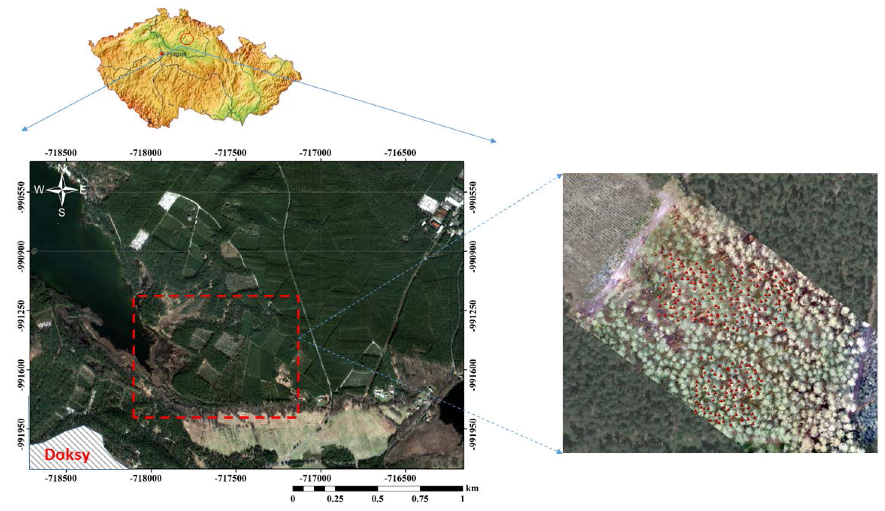
The Doksy territory lies on the shores of Lake Mácha in Northern Bohemia in the Czech Republic (Figure 1). The lake is largely surrounded by dense forests covering an area of 300 km². Geologically, the area is characterized by sandstone pseudokarst in the late stages of development, and the soils are either sandy or peaty, with shallow, peaty basins over rocky sandstone hummocks and sporadic volcanic hills. We selected three evenly-aged (managed stands) 40 × 40 m experimental plots and sampled all trees in each plot to estimate the tree heights, DBH, crown diameters, and stem volume. All plots were located northeast of the city of Doksy (−718000, −991250 NW to −717000, −991950 SE in the local coordinate system S-JTSK/Krovak East North, Figure 1). The research was carried out in a 140-year-old Pinus sylvestris L. (Scots pine) monoculture natural stand established on sandy soils (68%). The vegetative period tends to be rather warm and dry. The mean annual air temperature is 7.3 °C and the average annual maximum temperature is 31.5 °C. The mean annual precipitation is 635 mm, with only 354 mm during the growing season.

2.2. Field Survey

For the acquisition of field measurements, we used field-map technology. Field-map is a software and hardware product which combines flexible real-time geographic information system (GIS) software field-map with electronic equipment of high accuracy for mapping and dendrometric measurement. For this study, the dendrometric device which we used was the TruPulse 360/B laser range finder by lnc. Centennial, Colorado, USA. For the purpose of this study, we used the TruPulse 360/B to measure (i) the positions of individual trees by distance based on the field triangulation approach, (ii) tree heights based on the functionality of the digital relascope, and (iii) the mean of the horizontal widths of the tree crown radius in four orientations (east, west, north, and south). The coordinate system was set to S-JTSK/Krovak East North (a local coordinate system that is mainly used in the vicinity of the Czech Republic). The whole data collection process is rather ergonomic since mapped data can be seen simultaneously in the monitor of the computer in the form of layers (either point, lines, or polygons). Each layer can have a number of attributes (i.e., tree positions, heights, etc.) which are stored in a fully relational database.

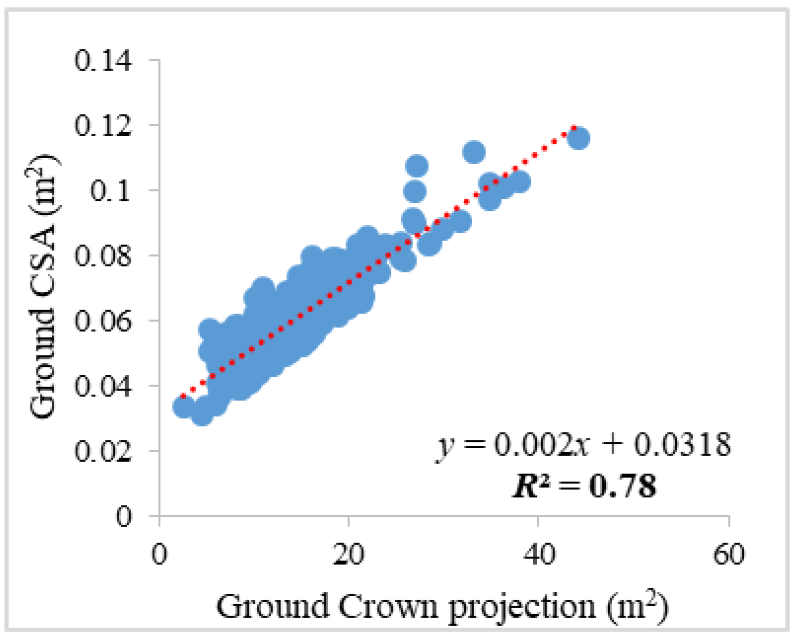
In addition, the DBH of trees (1.3 m above ground) was measured by a Häglof digital caliper (Häglof Sweden AB, Långsele, Sweden) in two perpendicular directions. Diameters were then transferred via bluetooth to the field-map computer and stored in the relative database. We considered the mean of measured diameters at breast height for computing the CSA. Finally, all the data was extracted by connecting the field-mapper with a universal serial bus (USB) to the personal computer (PC) for further processing. All field measurements were taken in November, 2015. In total, we sampled 223 live trees from all three plots.

2.3. Aerial and Satellite Imagery

The UAV data were acquired in March 2016. The platform model used was an octocopter SteadiDrone EI8HT, ready to fly (RTF) embedded with an RGB (red, green, blue) high-resolution camera. The camera was a Sony Alpha 6000 with an adjusted focal length of 25 mm. The octocopter needed approximately 7 min to complete a flight for each plot based on the predefined parameters (e.g., the number of waypoints) and the flight mode was set to semi-automatic. The flight path lines covered the entire study area and produced a set of images of the area. The octocopter was guided by a DJI (Dà-Jiāng Innovations Science and Technology Company, Shen Zhen, China) ground station, which is a global positioning system (GPS) flight planning and waypoint-based autopilot software. We performed three flights in total, one flight per plot, at a height of approximately 70 m above the ground with 80% frontal overlap and 70% side overlap.

In order to improve the accuracy of the 3D model, we also set up four ground control points (GCPs) randomly distributed within each plot; these points were measured using the Leica real-time kinematic (RTK) system, model RX1250XC with centimeter accuracy. Due to the low image quality, four of the 596 original images were excluded from the alignment process. During the alignment process, we set the accuracy to high for optimization of the final 3D model. We used Agisoft Photoscan© software (V 1.2.6, St. Petersburg, Russia) to construct the digital terrain model (DTM) and DSM from the 3D model with a cell size of 0.01 × 0.01 m. The reconstructed mesh of the 3D model was based on automatic classification on certain point classes through the triangulated irregular network (TIN) method. Due to the relatively open canopy in large parts of the study area, small bushes were often abundant in the understory, and, therefore, we classified them as ground points. For setting the parameters for the automatic classification, due to the presence of small bushes near the trees, we decreased the maximum angle from 15 (default value) to 11, the maximum distance from 4 to 1.5 m, while the cell size remained the same. All of the processing was conducted by one computer operator using an Intel^® Core™ i7-6700K with a base clock of 4 GHz and 32 GB random access memory (RAM) running with the Windows 10 Professional Edition 64-bit operating system.

We used the Pléiades 1A satellite (launched 16 December 2012) to acquire the space-borne image. The image was taken 27 March 2016, and it had 20 bits/pixel dynamic range of acquisition. For this study, we used one frame with a total area of 25 km² (5 × 5 km). The image consisted of four multispectral bands: RGB, infrared (IR), and one panchromatic (PAN), as can be seen in

Table 1. Pleiades-1A satellite sensor characteristics [17].

Imagery Products	Panchromatic: 50-cm resolution, black and white
	2-m multispectral (RGB—red, green, blue)
	Bundle: 50-cm black and white and 2-m multispectral
Spectral Bands	Panchromatic: 480–830 nm
	Blue: 430–550 nm
	Green: 490–610 nm
	Red: 600–720 nm
	Near Infrared: 750–950 nm
Image Location Accuracy	With ground control points: 1 m
	Without ground control points: 3 m (CE90)

. We used six GCPs for georeferencing the satellite image. For point acquisition, we used GPS RTK Leica model RX1250XC with a maximum error of two centimeters. The RTK correction was carried out by using a base/rover set, which sends and receives fast-rate over-the-air RTK data corrections, using the PDLGFU15 radio module.

Also, dark object correction was used to derive atmospheric optical information for radiometric normalization using the minimum digital number (DN) value of satellite images = water.

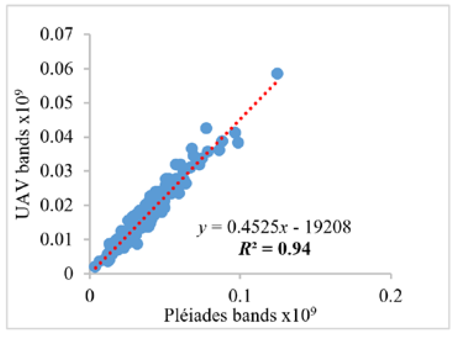
Normalized values of each band (RGB) from the UAV and satellite were then used to compare the spectral data (DN) between the UAV and Pléiades bands (separately) at the individual tree level using Equation (1):

$$Z_i=\frac{x_i-x_{\min }}{x_{\max }-x_{\min }}$$

(1)

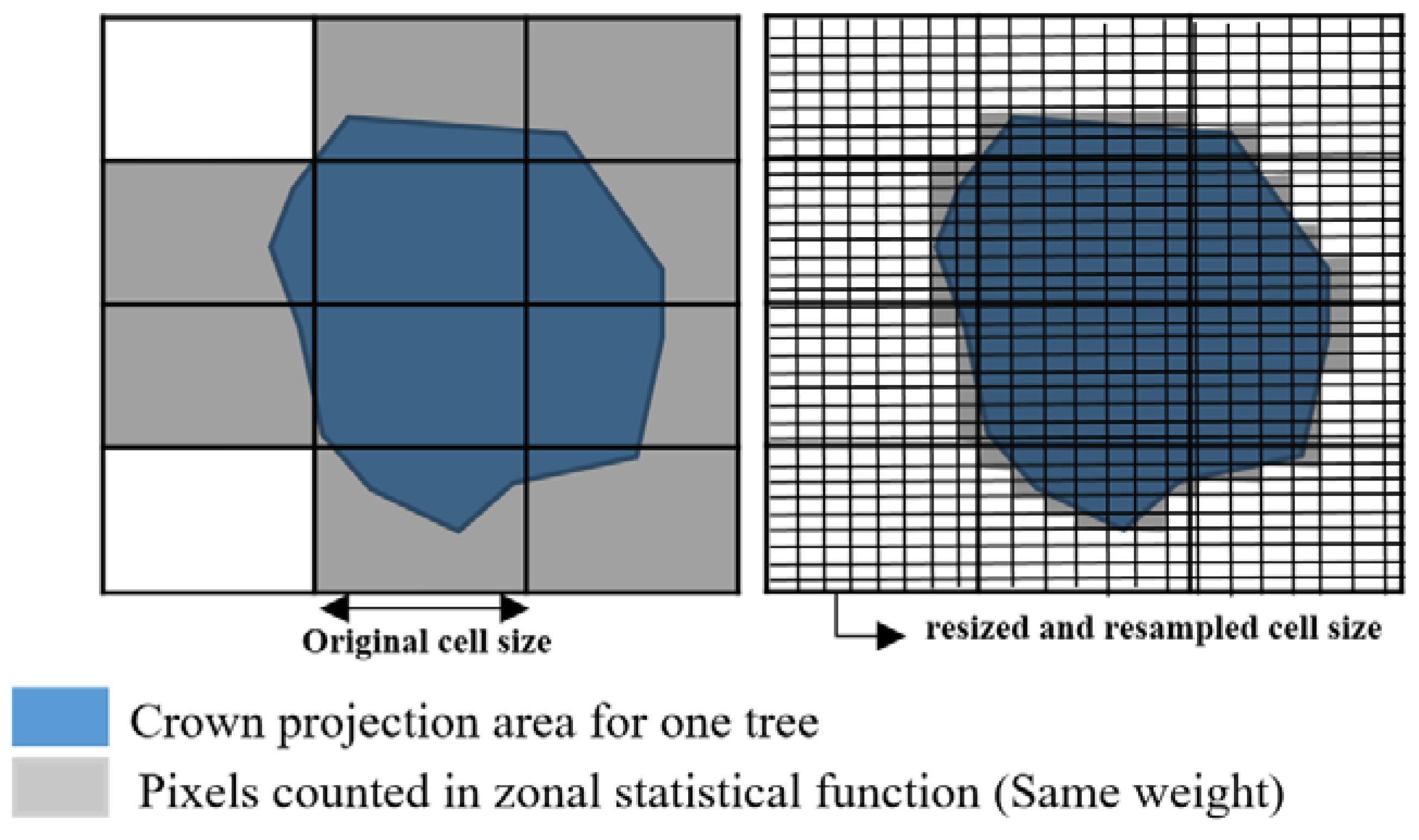
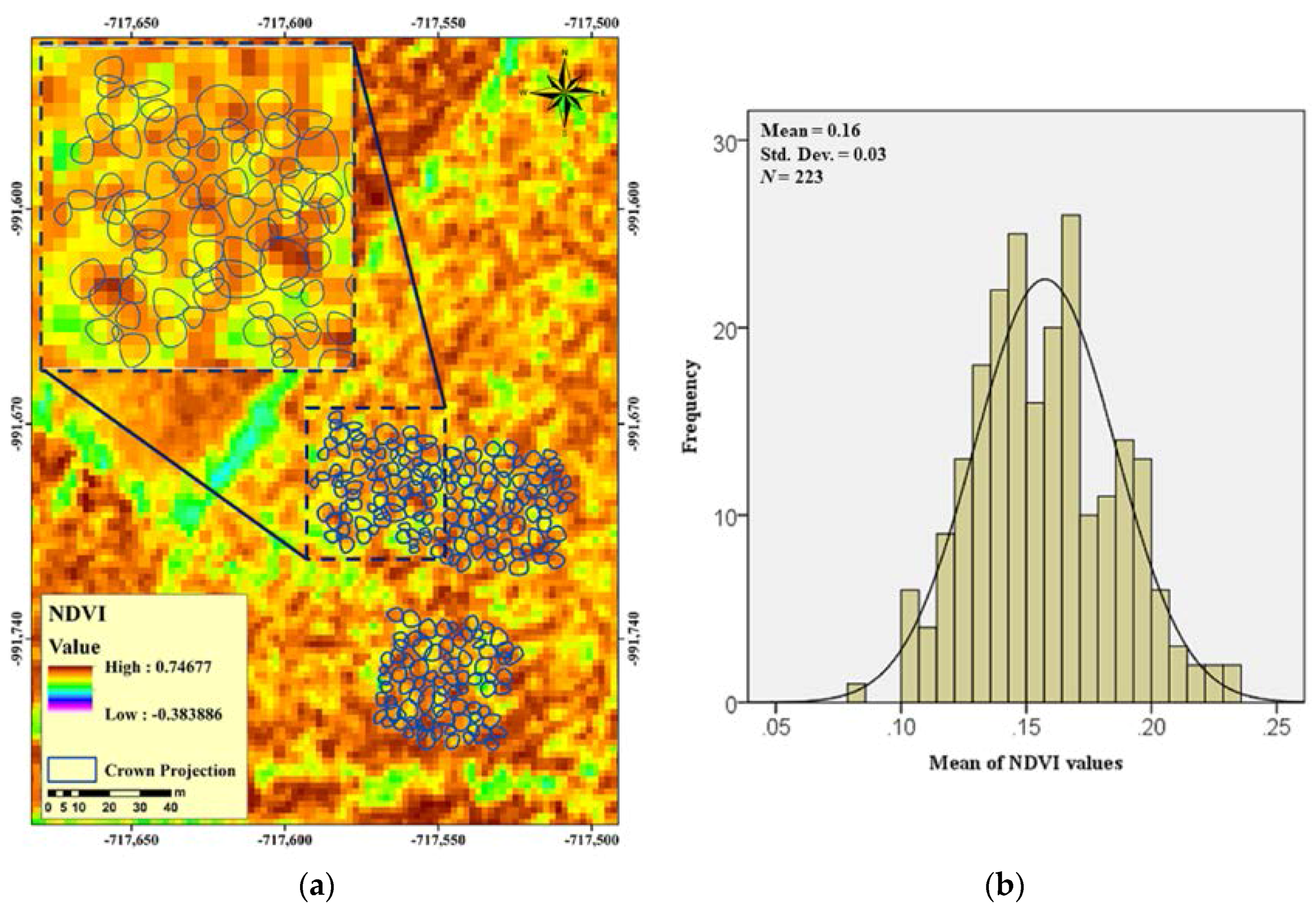
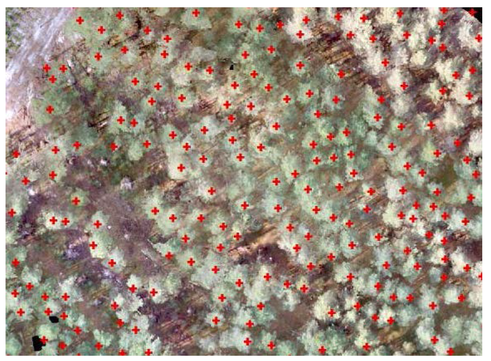
where Z_i describes the normalized data between 0 and 1, $x_i$ describes the spectral data (for both the UAV and satellite), and x_max and x_min are the maximum and minimum value for each band, respectively. In addition, using the nearest neighbor method, we resampled all three multi-spectral bands from the satellite from 2 m to 1 cm to assign more weight to pixels that cover more crown area (Figure 2). For extracting the spectral data (UAV and satellite), we used zonal statistics in ArcGIS desktop V.10.4.1 (ESRI Inc., Redlands, CA, USA), with the crown area for each individual tree as the zonal layer. We considered the same weight for averaging the DN values of pixels within the zonal layer.

To evaluate the greenness of the detected trees from the UAV and eliminate the dry trees and gap areas, the normalized difference vegetation index (NDVI) was used as a detector index (Equation (2)). This index is usually used to determine the visible spectral response by defining the ratio of greenness per individual tree applied to satellite data [18]:

$$\mathrm{NDVI}=\frac{NIR-R}{NIR+R}$$

(2)

where NIR stands for near-infrared and R refers to the red band.

2.4. Estimation of Height

To extract the height from the UAV, we computed the CHM, which was derived from the subtraction of the DSM from the DTM. The local maxima algorithm was then used to estimate the height; this algorithm enhances the maximum value within a specified kernel size. As a first step, we used the focal statistics tool in ArcGIS to identify the highest pixel value using the CHM as the input data layer. We performed a low-pass filter to reduce the noise effect and regulate the values of the smoothing window [19]. Among the several processing types we tested in different variances of radius using circular-shaped areas, the best results were at a kernel size with a radius of 1 m based on the average crown diameter derived from the ground measurements (Figure 3). For matching the pixel values, we used the conditional if/else statement on each of the input cells of CHM and focal statistics results, by entering the following command “Con (“CHM” = “focal statistics result”, 1)” using the ArcGIS V. 10.4.1 (ESRI, Redlands, CA, United States) raster calculator.

This conditional tool performs an if/else statement on each input cell and it returns a binary layer with a value of zero assigned as no data and a value of one for data. Finally, the return value was the value when the CHM value equaled the focal statistics output.

2.5. Estimation of Crown Projection

For the extraction of the crown area, we used the method of inverse watershed segmentation (IWS), as proposed by Panagiotidis et al. [20]. To implement the IWS, we multiplied the CHM model by −1 so that treetops would appear as ponds and crowns as watersheds. Then, we created a flow direction layer for creating hydrological drainage basins [21]. We applied the ArcGIS reclassify tool on the CHM to create a Boolean layer comprised of two categories; we used a threshold value of 15 m as the classification delimiter. Essentially, that means that pixels with values above 15 m were assigned with a value of 1, and those that were lower than 15 m were assigned a value of 0. Afterwards, the CHM was converted to polygons; the center of each polygon was identified, the polygons were converted to lines, and the lines to points. This allowed us to assign points to the periphery of each polygon. Finally, we used the ArcGIS “zonal geometry as table” tool to define individual tree crown diameters.

2.6. Estimation of Cross-Sectional Area and Stem Volume

To estimate the CSA and volume of individual trees, the coefficient of determination (R²) between the crown diameter and DBH was calculated. The formula of this coefficient was then used to measure the CSA, by replacing the measured crown size (ground) with the crown size extracted from the UAV. Once we had defined the height and CSA, we were able to estimate the stem volume from the UAV. Additionally, for modelling the stem volume, we considered the shape of tree stems as cylinders.

2.7. Extrapolation of Tree Attributes

We were able to calculate calibrated equations that can be used to determine tree attributes such as CSA and stem volume directly using the spectral information from Pléiades for each tree based on the following equations: linear relation between the UAV spectral data and tree parameters such as CSA and volume (Equation (3)) and linear relation between the UAV and Pléiades spectral data (Equation (4)). In details:

CSA = AX₁ + B

(3)

X₁ = CX₂ + D

(4)

where CSA is cross-section area, X₁ is UAV spectral data, and X₂ is satellite spectral data.

By replacing X₁ in Equation (3) with the Equation number (4), we will be able to measure the CSA directly by satellite spectral data using the below equation:

CSA = A(CX₂ + D) + B

(5)

2.8. Statistical Evaluation and Validation of Data

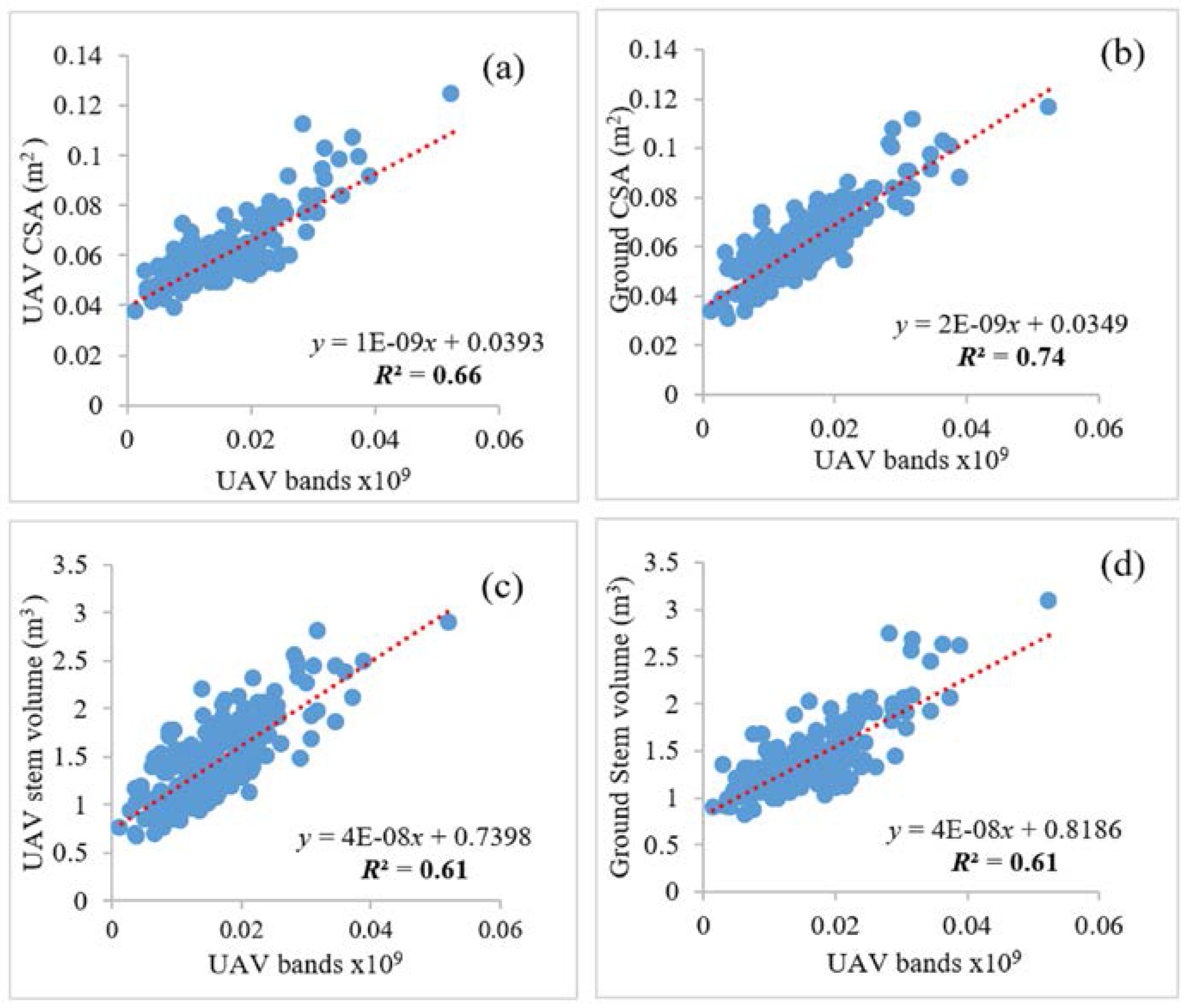
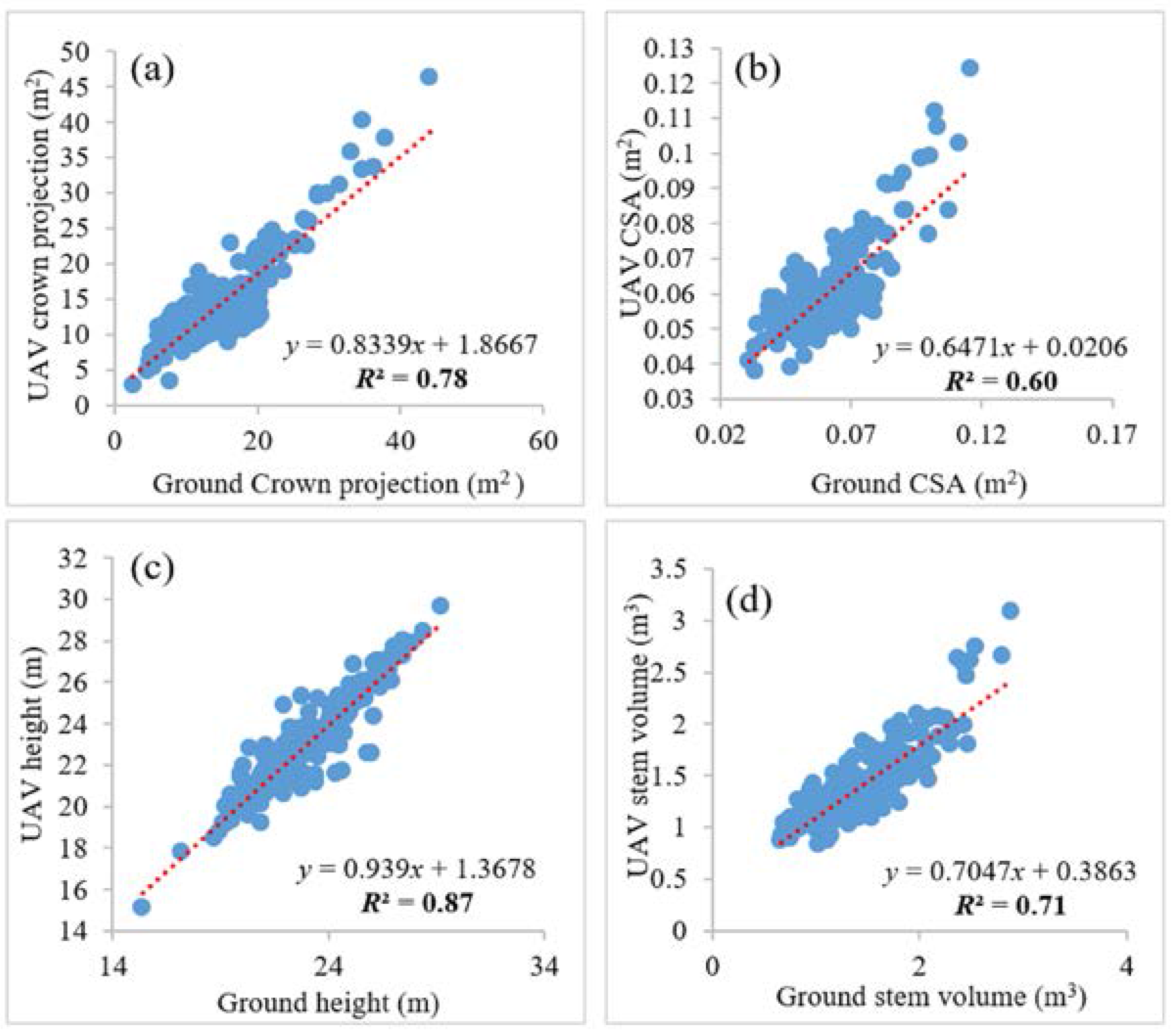
All statistical analyses were conducted in IBM SPSS V.24 (64-bit 2016) and Excel (Microsoft^® Office). The linear regression was used to study correlation between the ground data and tree parameters predicted by the UAV.

Pearson correlation coefficient was computed to analyze the relationships between the spectral values of the UAV RGB bands and tree parameters derived from ground inventory and UAV in two different probability values (p < 0.05 and p < 0.01). In this study, due to the lack of an IR band in the UAV approach, we computed the vegetation index (VI) [22], green-red vegetation index (GRVI) [22], and visible atmospherically-resistant index, green (VARI g) [23] using the following equations:

$$\mathrm{VI}=\frac{\mathrm{Green}}{\mathrm{Red}}$$

(6)

$$\mathrm{GRVI}=\frac{\left(\mathrm{Green}-\mathrm{Red}\right)}{\left(\mathrm{Green}+\mathrm{Red}\right)}$$

(7)

$$\mathrm{VARI}\mathrm{g}=\frac{\left(\mathrm{Green}-\mathrm{red}\right)}{\mathrm{Green}+\mathrm{Red}-\mathrm{Blue}}$$

(8)

3. Results

For the sake of simplicity, we divided the results into three parts. In the first part, we presented an overview of tree characteristics in our study area. In the second part, we mainly focused on the potential of the UAV platform deployed with an RGB camera to act as an accurate, alternative field measurement technique. In the third part, we tried to extrapolate the extracted data from the UAV to a larger forested area based on spectral correlation between Pléiades and the UAV.

3.1. General Evaluation of the Study Area

The evaluation of tree attributes showed similarities between the sample plots. However, there was a difference between the variability of sample plots, whereas plot 1 had a lower amount of variability compared with the other two plots (

Table 2. Descriptive statistics of the three plots based on ground survey.

Sample	Index	Crown Projection (m2)	DBH (m)	CSA (m2)	Height (m)	Volume (m3)
Plot 1 N = 74	Mean	15.24	0.28	0.06	21.23	1.30
	Variability	30.61	0.15	0.06	7.00	1.30
	Std.	5.20	0.03	0.01	1.33	0.30
Plot 2 N = 72	Mean	14.71	0.28	0.06	23.03	1.43
	Variability	41.54	0.17	0.08	13.80	2.10
	Std.	7.75	0.04	0.02	2.24	0.46
Plot 3 N = 77	Mean	14.94	0.28	0.06	24.49	1.56
	Variability	28.67	0.17	0.08	8.20	2.13
	Std.	6.45	0.03	0.02	2.00	0.45
Total N = 223	Mean	14.97	0.28	0.06	22.96	1.43
	Variability	41.54	0.18	0.08	13.80	2.21
	Std.	6.51	0.03	0.01	2.32	0.42

Std. = standard deviation; DBH = diameter at breast height; CSA = cross-sectional area.

).

In addition, the NDVI showed that the mean greenness of trees ranged from 0.3 to 0.55 (Figure 4); this range is associated with shrubs-grasslands and temperate forest land-cover classes [24].

3.2. UAV Performance

Linear regression (Figure 5) exhibited a strong relationship in the significant level of α = 0.05 (R² = 0.78) between the cross-section area and crown projection derived from ground data with a root mean square error percent (RMSE%) = 11.35 (

Table 3. Statistical summary table, where ID represents the simplicity of identification of each tested regression; N: number of observations; RMSE: root mean square error; and df: degrees of freedom. ID represents the simplicity of identification of each tested regression.

ID	N	RMSE	RMSE%	Bias	Bias %	df	p-Value
1	223	0.0069	11.35	0.0018	2.96	222	0.00
2	223	3.14	20.96	-	-	222	0.00
3	223	0.01	15.24	-	-	222	0.00
4	223	0.86	3.73	-	-	222	0.00
5	223	0.23	15.88	-	-	222	0.00

ID 1 indicates the relation between the ground CSA versus ground crown projection; ID 2 indicates the relation between the crown projection derived from UAV and ground data; ID 3 indicates the relation between the CSA derived from the UAV and ground data; ID 4 indicates the relation between the estimated height from the UAV and ground data; and ID 5 indicates the relation between the stem volume derived from the UAV and ground data.

; ID = 1). For the crown projections, a strong relationship (R² = 0.78; Figure 6a) between the ground and UAV data was observed with an RMSE% = 20.96 (Table 3; ID = 2). Based on these results, we were able to estimate cross-sectional areas from the UAV using adjusted R and RMSE% with an R² = 0.60 (Figure 6b) and RMSE% = 15.24 (Table 3; ID = 3). Additionally, the results of the height estimation showed strong correlation between the ground and extracted data from the UAV with an R² = 0.87 (Figure 6c) and RMSE% = 3.73 (Table 3; ID = 4). Finally, we calculated the stem volume based on data from the UAV and the ground. The comparison of the stem volume between the ground and UAV data showed significant correlation with R² = 0.71 (Figure 6d) and RMSE% = 15.88 (Table 3; ID = 5).

Moreover, the results of the correlation coefficient indicated that the most important descriptive statistic index for all models was the sum of the spectral data as can be seen in

Table 4. Pearson correlation between the UAV spectral descriptive data and tree attributes at the level of individual trees.

Tree Parameter	Min	Max	Mean	Std.	Sum	Median
CSA (Ground)	−0.208 **	0.133 *	0.224 **	0.160 *	0.864 **	0.229 **
Stem volume (Ground)	−0.200 **	0.131	0.239 **	0.180 **	0.795 **	0.255 **
CSA (UAV)	−0.140 *	0.0641	0.055	0.012	0.821 **	0.049
Stem volume (UAV)	−0.158 *	0.072	0.107	0.05	0.795 **	0.115

** Correlation is significant at the 0.01 level (two-tailed). * Correlation is significant at the 0.05 level (two-tailed).

. Finally, our results showed that vegetation indicators that were computed using RGB bands had a significant correlation at the level of α = 0.01 with the individual tree stem volume, as can be seen in

Table 5. The Pearson correlation coefficient between the different vegetation indicators derived from UAV and tree attributes at the level of individual trees. VI: vegetation index; GRVI: green-red vegetation index; and VARI g: vegetation atmospherically resilient index, green.

Vegetation Index	CSA (Ground)	Stem Volume (Ground)	CSA (UAV)	Stem Volume (UAV)
VI	0.103	0.208 **	0.110	0.218 **
GRVI	−0.106	−0.210 **	−0.113	−0.221 **
VARI g	−0.106	−0.211 **	−0.112	−0.221 **

** Correlation is significant at the 0.01 level (two-tailed).

.

The selection process for the best independent variable for further analysis was based on the largest positive or negative correlations with the dependent variables. Based on our results, we chose the sum of pixel values as an independent variable to calculate the regression between the spectral data and tree attributes (Figure 7). Our results showed there was high correlation between the UAV main bands and tree attributes based on R² (Figure 7).

3.3. UAV-Pléiades Extrapolation

Overall, our findings indicated that there is a strong relationship between the UAV and Pléiades spectral data with an R² = 0.94 (Figure 8). Based on the regression model equations (Figure 7 and Figure 8), we were able to calculate calibrated formulas that could determine tree attributes, such as CSA and stem volume (

Table 6. Basic errors of CSA and volume based on extrapolated data.

Index	CSA	Volume
RMSE	0.018	0.21
RMSE%	30.56	31.01
Bias	−0.015	−0.39

), directly by using the spectral information from Pléiades for each tree. Formulas presented in Table 6 were used to extrapolate the extracted data from the UAV to a larger area based on satellite spectral information.

Our results showed that the computed formulas (9 and 10) could be used for the extrapolation of CSA and volume at the individual tree level with significant accuracy, as can be seen in Table 6. In addition, Figure 9 indicates that there were no significant differences between the mean of CSA and volume derived from UAV and ground data. Also, the same figure and Table 6 show that the extrapolation method has estimated the tree parameters with reasonable accuracy.

CSA = 1 × 10⁻⁹ (0.4525x − 19208) + 0.0392

(9)

Volume = 4 × 10⁻⁸ (0.4525x − 19208) + 0.7398

(10)

where the x is the spectral information derived from satellite imagery.

4. Discussion

Many studies have provided good examples of 3D model reconstructions of VHR DSMs from UAV-based imagery to systematically observe forest attributes, such as tree crown, tree height, and DBH [25,26]. Structural forest attributes are commonly extracted from the CHM using regression models to predict tree characteristics for forest inventory purposes [27]. Detailed CHMs from remote sensing data have recently gained more attention because they can be used to efficiently predict key forest parameters, such as tree height, crown projection, and stem volume. In this study, it was demonstrated that a consumer-grade camera deployed on a UAV platform generated a 3D scene of the entire study area, which was used to quantify single-tree parameters based on automatic and semi-automatic methods that can be used to support detailed construction or update existing forest inventories. Of course, this is just one of the basic reasons why UAVs are gradually replacing conventional field measurements. However, some applications require more accurate results in terms of absolute means, and this low-cost aerial approach would, therefore, require the collection of ground truth data to ensure this.

Based on the linear regression and RMSE results, we concluded that there is generally a high correlation between estimated (UAV) and observed data (ground) (Table 3; Figure 5 and Figure 6). In this particular study, the methodological approach and the algorithms that were used to determine tree heights and crown diameters were influenced by the relative homogeneity of the study area; all trees were of similar age and had similar morphological characteristics (Table 2). Aslo, as it can be seen in Figure 9, the amount of CSA and volume for 50% of the trees distributed around the median, but the remaining 50% were distributed in a wider range.

In general, estimation of forest parameters in homogeneous forests is preferable for the application of algorithms, such as local maxima and IWS, because homogeneous forests allow for higher precision using a single kernel size method for smoothing the CHM [20,28,29]. It is evident that the UAV can be used to efficiently estimate heights and crown diameters (Figure 6a–c, and Table 3).

Since there was a high correlation between the crown and DBH from the ground measurements (Figure 5), and due to the fact that UAVs can be used to estimate both heights and crown diameters, there is a possibility for indirect measurement of stem diameters (Figure 6b and Table 3; ID 3) and volume (Figure 6d and Table 3; ID 5) [30].

Additionally, we evaluated the relationship between the tree parameters (CSA and stem volume of individual trees) and the spectral information that was extracted from the UAV imagery. Our results showed that there is a significant correlation between the CSA and stem volume and spectral/textural values derived from the UAV. These results are similar to the results of several studies that have emphasized the possibility of the estimation of tree/stand parameters, such as basal area (BA) and volume, using spectral (main bands) and textural (vegetation indicators) values of aerial/satellite images [31,32,33]. For the vegetation index (VI), a low value for this attribute implies lower density and stem volume, while higher values indicate dense canopy and higher stem volumes. This explains the positive correlation that we found between the VI, CSA, and stem volume in our study. This result is in accordance with the results of Wallner et al. [31].

The inverse relation between the stem volume and VARI g and GRVI indicators (Table 5) can be explained as follows: due to the fact that vegetation absorbs more red light and reflects more green light, a high value in the red band indicates less vegetation occurrence, which can be explained by the negative correlation between (i) VARI g and GRVI, and (ii) CSA and stem volume.

Finally, our results showed that spectral reflection of individual trees from both Pléiades and the UAV had a high correlation of more than 90% (Figure 8). Based on this finding, high-resolution satellite imagery can be used to extrapolate areas that cannot be reached with a UAV. However, the described methodology can be applied only in the case where the areas present similar structural characteristics. Although the extrapolation process in our study caused underestimation of tree parameters compared to that of ground data and UAV (Figure 9), the suggested methodology can be used for practical forestry and can open up new scientific areas of extrapolation methods to inspire other researchers in the forest community. In future work, we plan to use auxiliary data such as environmental data (edaphic, climatic, and topographic) in order to be able to enhance the methodology for homogeneous areas and to calibrate and assess the methodology in the case of diverse forested areas. For areas with higher variability, one suggestion is to divide the whole area into more homogenous areas, through the construction of homogenous groups or classes. We also assume that the use of hyperspectral sensors can lead to a better result with higher accuracy.

5. Conclusions

In this study, we proposed a method to test the performance of UAV image-based point clouds to accurately estimate tree attributes. For this purpose, detection algorithms based on high-quality CHM were used. To potentially improve the results of the 3D image reconstruction model and ensure the integrity of the results based on CHM, we used four GCPs, measured with RTK GPS. Many studies have previously treated estimates of tree parameters, such as tree crown delineation and treetop detection, as two separate procedures [28]. We extrapolated the estimated data from the UAV to a larger area based on a significant correlation (R-squared values and Pearson correlation percentages were greater than 0.90) between the spectral data from UAV and Pléiades. This study demonstrated that it is possible to use calibrated (linear regression) formulas (Table 6) to extrapolate data into larger forested areas (downscaling). Precision forestry is focusing on the use of high-resolution data to support site-specific tactical and operational decision-making (e.g., area productivity) over large forest areas. Therefore, the application of this study, as well as other similar studies, should be explored in the content of the European Common Policy to assess the full potential of these methods for covering larger forested areas.

Regarding the performance of remote sensing versus field measurements, based on our empirical data, we can conclude that the positive comparisons between reference ground measurements and remote sensing estimation of tree attributes confirmed the potential of the workflow process that can be applied as a quick and effective alternative technique to characterize forest tree parameters.

References

1. Järnstedt, J.; Pekkarinen, A.; Tuominen, S.; Ginzler, C.; Holopainen, M.; Viitala, R. Forest variable estimation using a high-resolution digital surface model. J. Photogramm. Remote Sens. 2012, 74, 78–84. [Google Scholar] [CrossRef]
2. Straub, C.; Stepper, C.; Seitz, R.; Waser, L.T. Potential of UltraCamX stereo images for estimating timber volume and basal area at the plot level in mixed European forests. Can. J. For. Res. 2013, 43, 731–741. [Google Scholar] [CrossRef]
3. White, J.C.; Wulder, M.A.; Vastaranta, M.; Coops, N.C.; Pitt, D.; Woods, M. The utility of image-based point clouds for forest inventory: A comparison with airborne laser scanning. Forests 2013, 4, 518–536. [Google Scholar] [CrossRef]
4. Stepper, C.; Straub, C.; Pretzsch, H. Using semi-global matching point clouds to estimate growing stock at the plot and stand levels: Application for a broadleaf-dominated forest in central Europe. Can. J. For. Res. 2014, 45, 111–123. [Google Scholar] [CrossRef]
5. Carleer, A.P.; Debeir, O.; Wolff, E. Assessment of Very High Spatial Resolution Satellite Image Segmentations. Photogramm. Eng. Remote Sens. 2005, 71, 1285–1294. [Google Scholar] [CrossRef]
6. Edson, C.; Wing, M.G. Airborne Light Detection and Ranging (LiDAR) for Individual Tree Stem Location, Height, and Biomass Measurements. Remote Sens. 2011, 3, 2494–2528. [Google Scholar] [CrossRef] [Green Version]
7. Popescu, S.C.; Wynne, R.H.; Nelson, R.F. Measuring Individual Tree Crown Diameter with Lidar and Assessing Its Influence on Estimating Forest Volume and Biomass. Can. J. For. Res. 2003, 29, 564–577. [Google Scholar] [CrossRef]
8. Tomppo, E.; Olsson, H.; Ståhl, G.; Nilsson, M.; Hagner, O.; Katila, M. Combining national forest inventory field plots and remote sensing data for forest databases. Remote Sens. Environ. 2008, 112, 1982–1999. [Google Scholar] [CrossRef]
9. McRoberts, R.E.; Cohen, W.B.; Næsset, E.; Stehman, S.V.; Tomppo, E.O. Using remotely sensed data to construct and assess forest attribute maps and related spatial products. Scand. J. For. Res. 2010, 25, 340–367. [Google Scholar] [CrossRef]
10. Shao, Z.; Zhang, L. Estimating Forest Aboveground Biomass by Combining Optical and SAR Data: A Case Study in Genhe, Inner Mongolia, China. Sensors 2016, 16, 834. [Google Scholar] [CrossRef] [PubMed]
11. Lehmann, J.R.K.; Nieberding, F.; Prinz, T.; Knoth, C. Analysis of Unmanned Aerial System-Based CIR Images in Forestry—A New Perspective to Monitor Pest Infestation Levels. Forests 2015, 6, 594–612. [Google Scholar] [CrossRef] [Green Version]
12. Kayitakire, F.; Hamel, C.; Defourny, P. Retrieving forest structure variables based on image texture analysis and Ikonos-2 imagery. Remote Sens. Environ. 2006, 102, 390–401. [Google Scholar] [CrossRef]
13. St-Onge, B.; Hu, Y.; Vega, C. Mapping the height and above-ground biomass of a mixed forest using LiDAR and stereo Ikonos images. Int. J. Remote Sens. 2008, 29, 1277–1294. [Google Scholar] [CrossRef]
14. Ozdemir, I.; Karnieli, A. Predicting forest structural parameters using the image texture derived from worldview-2 multispectral imagery in a dryland forest, Israel. Int. J. Appl. Earth Obs. Geoinf. 2011, 13, 701–710. [Google Scholar] [CrossRef]
15. Shamsoddini, A.; Trinder, J.C.; Turner, R. Pine plantation structure mapping usingWorldView-2 multispectral image. Int. J. Remote Sens. 2013, 34, 3986–4007. [Google Scholar] [CrossRef]
16. Immitzer, M.; Stepper, C.; Böck, S.; Straub, C.; Atzberger, C. Forest ecology and management use of WorldView-2 stereo imagery and National Forest Inventory data for wall-to-wall mapping of growing stock. For. Ecol. Manag. 2016, 359, 232–246. [Google Scholar] [CrossRef]
17. Astrium GEO-Information Services, Pléiades Imagery User Guide. Available online: http://www.cscrs.itu.edu.tr/assets/downloads/PleiadesUserGuide.pdf (accessed on 1 August 2012).
18. Surový, P.; Ribeiro, N.A.; Pereira, J.S.; Yoshimoto, A. Estimation of Cork Production Using Aerial Imagery. Rev. Árvore 2015, 39, 853–861. [Google Scholar] [CrossRef]
19. Pitkänen, J.; Maltamo, M.; Hyyppä, J.; Yu, X. Adaptive Methods for Individual Tree Detection on Airborne Laser Based Canopy Height Model. In Proceedings of ISPRS Working Group VIII/2: “Laser-Scanners for Forest and Landscape Assessment”; Theis, M., Koch, B., Spiecker, H., Weinacker, H., Eds.; University of Freiburg: Freiburg, Germany, 2004; pp. 187–191. [Google Scholar]
20. Panagiotidis, D.; Abdollahnejad, A.; Surový, P.; Chiteculo, V. Determining tree height and crown diameter from high-resolution UAV imagery. Int. J. Remote Sens. 2016, 38, 1–19. [Google Scholar] [CrossRef]
21. Wannasiri, W.; Nagai, M.; Honda, K.; Santitamont, P.; Miphokasap, P. Extraction of Mangrove Biophysical Parameters Using Airborne LiDAR. Remote Sens. 2013, 5, 1787–1808. [Google Scholar] [CrossRef]
22. Tucker, C.J. Red and Photographic Infrared Linear Combinations for Monitoring Vegetation. Remote Sens. Environ. 1979, 8, 127–150. [Google Scholar] [CrossRef]
23. Gitelson, A.; Stark, R.; Grits, U.; Rundquist, D.; Kaufman, Y.; Derry, D. Vegetation and Soil Lines in Visible Spectral Space: A Concept and Technique for Remote Estimation of Vegetation Fraction. Int. J. Remote Sens. 2002, 23, 2537–2562. [Google Scholar] [CrossRef]
24. Arulbalaji, P.; Gurugnanam, B. Evaluating the Normalized Difference Vegetation Index Using Landsat Data by Envi in Salem District, Tamilnadu, India. Int. J. Dev. Res. 2014, 4, 1844–1846. [Google Scholar]
25. Baltsavias, E.; Gruen, A.; Eisenbeiss, H.; Zhang, L.; Waser, L.T. High-Quality Image Matching and Automated Generation of 3D Tree Models. Int. J. Remote Sens. 2008, 29, 1243–1259. [Google Scholar] [CrossRef]
26. Dandois, J.P.; Ellis, E.C. Remote Sensing of Vegetation Structure Using Computer Vision. Remote Sens. 2010, 2, 1157–1176. [Google Scholar] [CrossRef]
27. Næsset, E. Predicting Forest Stand Characteristics with Airborne Scanning Laser Using a Practical Two-Stage Procedure and Field Data. Remote Sens. Environ. 2002, 80, 88–99. [Google Scholar] [CrossRef]
28. Wang, L.; Gong, P.; Biging, G.S. Individual Tree-Crown Delineation and Treetop Detection in High-Spatial-Resolution Aerial Imagery. Photogramm. Eng. Remote Sens. 2004, 70, 351–357. [Google Scholar] [CrossRef]
29. Jakubowski, M.K.; Li, W.; Guo, Q.; Kelly, M. Delineating Individual Trees from Lidar Data: A Comparison of Vector- and Raster-based Segmentation Approaches. Remote Sens. 2013, 5, 4163–4186. [Google Scholar] [CrossRef]
30. Tuominen, S.; Balazs, A.; Saari, H.; Pölönen, I.; Sarkeala, J.; Viitala, R. Unmanned aerial system imagery and photogrammetric canopy height data in area-based estimation of forest variables. Silva Fenn. 2015, 49, 1348. [Google Scholar] [CrossRef]
31. Wallner, A.; Elatawneh, A.; Schneider, T.; Knoke, T. Estimation of forest structural information using rapideye satellite data. Forestry 2015, 88, 96–107. [Google Scholar] [CrossRef]
32. Straub, C.; Weinacker, H.; Koch, B. A comparison of different methods for forest resource estimation using information from airborne laser scanning and CIR orthophotos. Eur. J. For. Res. 2010, 129, 1069–1080. [Google Scholar] [CrossRef]
33. Heiskanen, J. Estimating aboveground tree biomass and leaf area index in a mountain birch forest using ASTER satellite data. Int. J. Remote Sens. 2006, 27, 1135–1158. [Google Scholar] [CrossRef]
Figure 1. Location of the study area in the northern part of the Czech Republic in the local coordinate system S-JTSK/Krovak East North. Source: Google Earth (elaborated work in ArcGis for higher map detail).
Forests 09 00085 g001
Figure 2. Example of resampled pixels, from 2 m to 1 cm.
Forests 09 00085 g002
Figure 3. The applied method of local maxima seeds for the derivation of tree heights (red crosses show the detected treetops by the local maxima approach).
Forests 09 00085 g003
Figure 4. (a) The NDVI (normalized difference vegetation index) calculated for the study area and (b) the histogram of NDVI derived from Pléiades 1A satellite imagery.
Forests 09 00085 g004
Figure 5. The correlation between crown projection and cross-sectional areas.
Forests 09 00085 g005
Figure 6. The correlation of (a) crown projection between the ground and UAV (unmanned aerial vehicle) data in m2; (b) cross-sectional areas (CSA) between the ground and UAV data in m2; (c) height between the ground and UAV data in m; and (d) stem volume between the ground and UAV data in m3.
Forests 09 00085 g006
Figure 7. The relationship between spectral data of the UAV bands (×109) and tree characteristics: (a) UAV cross-section area in m2; (b) ground cross-section area in m2; (c) UAV stem volume in m3; and (d) ground stem volume in m3.
Forests 09 00085 g007
Figure 8. The relationship between spectral data between the UAV and Pléiades bands (×109).
Forests 09 00085 g008
Figure 9. Box-and-whisker plots for comparison of the differences between the means of tree parameters: (a) CSA (m2) (b) Volume (m3) derived from different approaches. The medians of the measured values are marked by vertical lines inside the boxes. The ends of the boxes are the interquartile range (upper: Q3 and lower: Q1). The whiskers show the highest and lowest observations.
Forests 09 00085 g009