Relative Contributions of Solubility and Mobility to the Stability of Amorphous Solid Dispersions of Poorly Soluble Drugs: A Molecular Dynamics Simulation Study


Abstract
1. Introduction
2. Methods
2.1. Force Field
2.2. Molecular Dynamics Simulations
2.3. Analysis
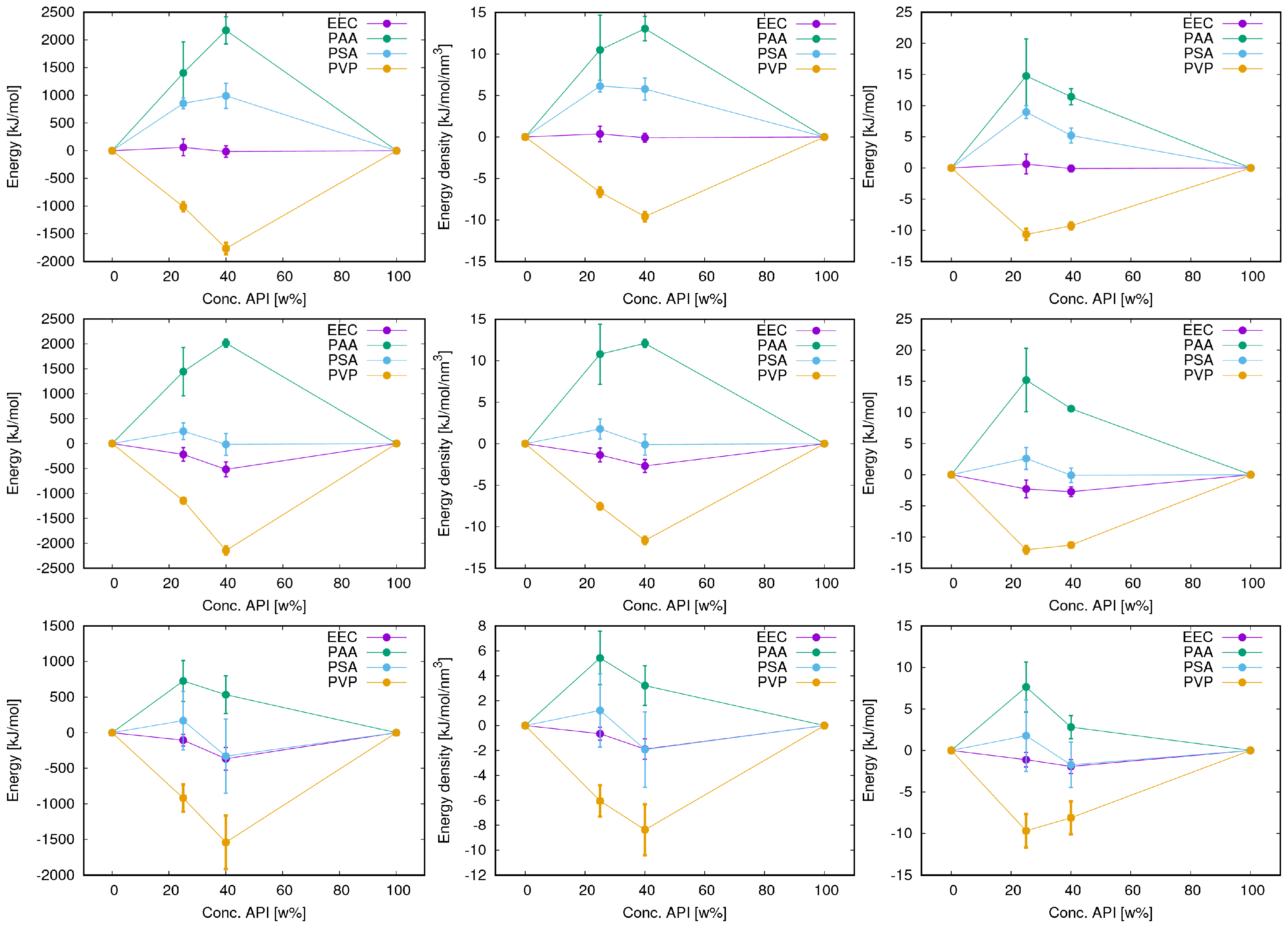
3. Results
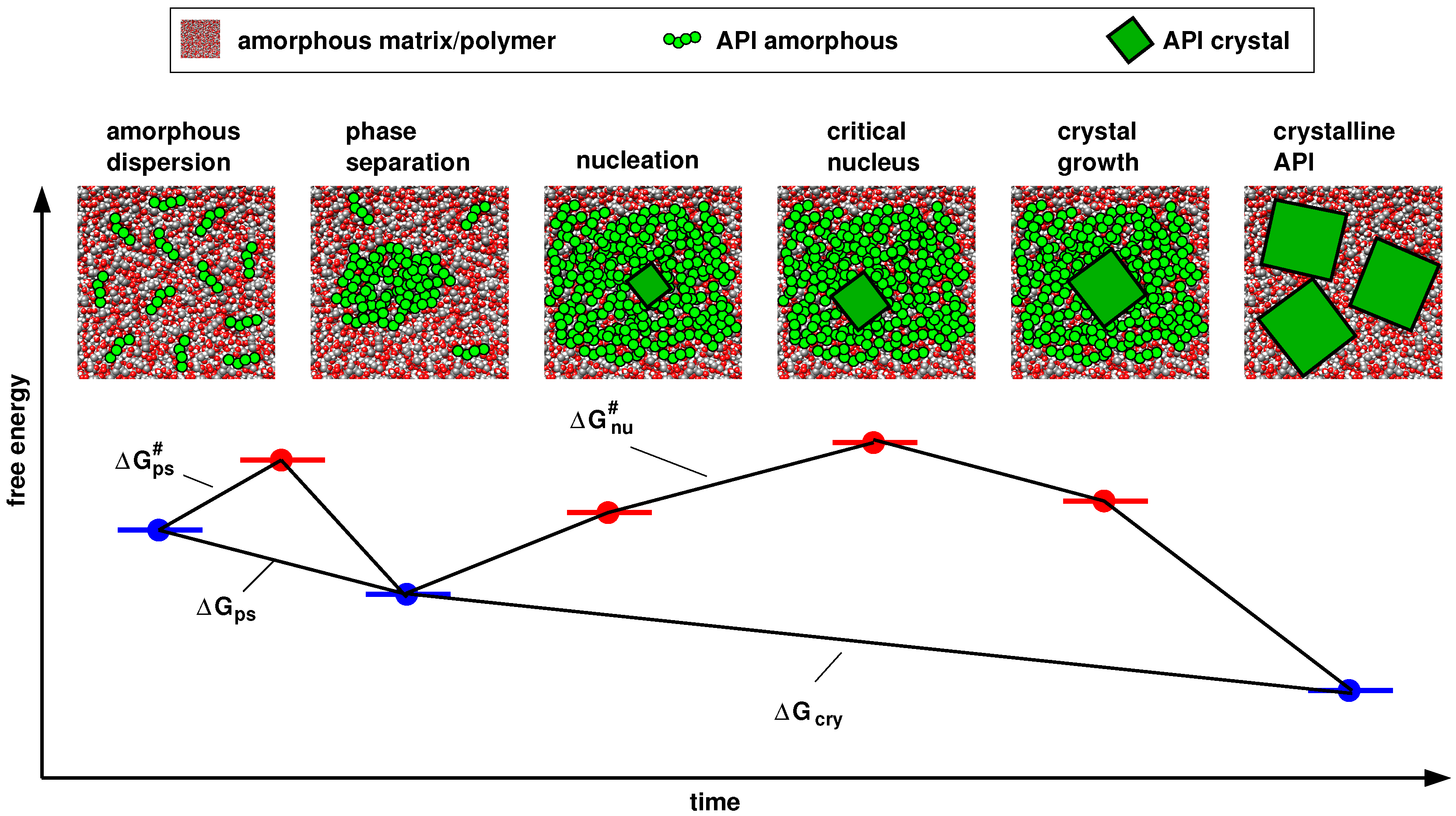
3.1. Choice of Model Systems
3.2. Convergence
3.3. Energy Terms and Trends
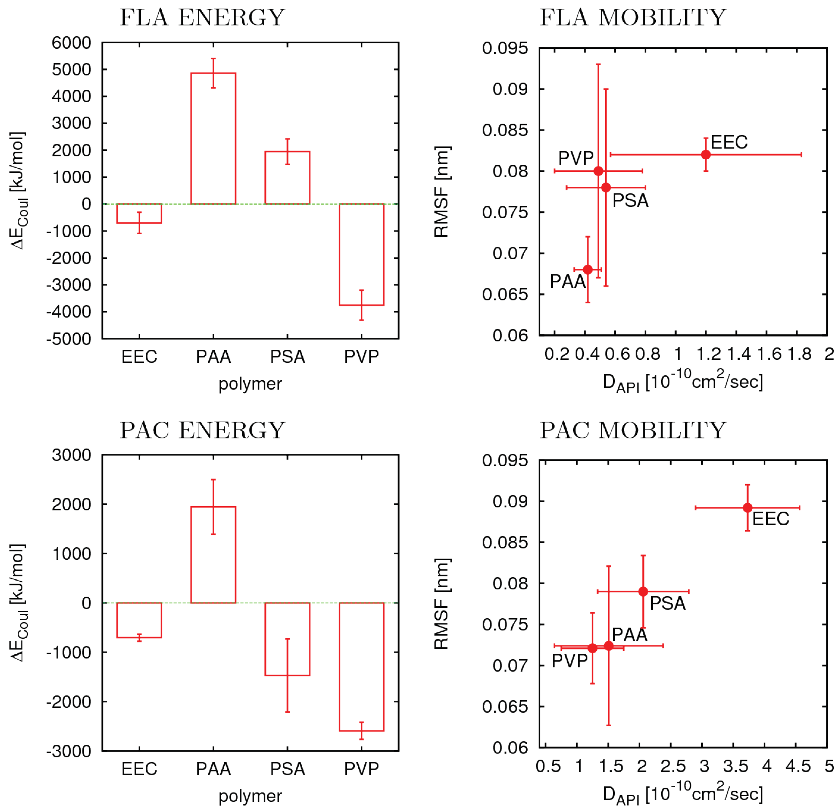
3.4. Flufenamic Acid
3.5. Phenacetin
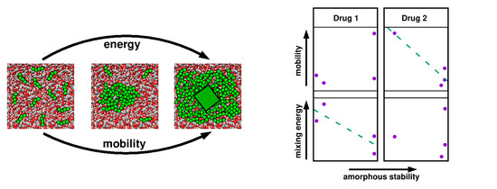
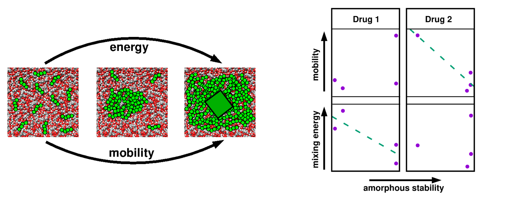
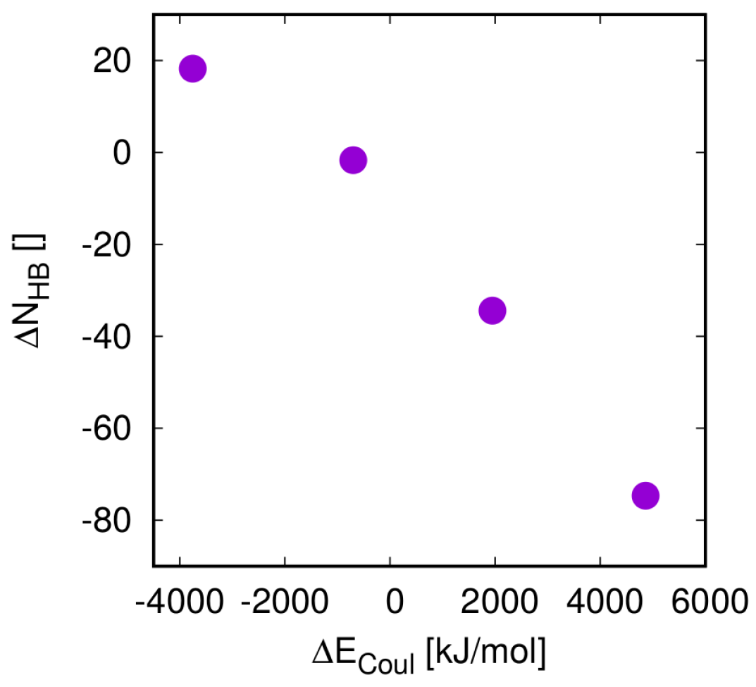
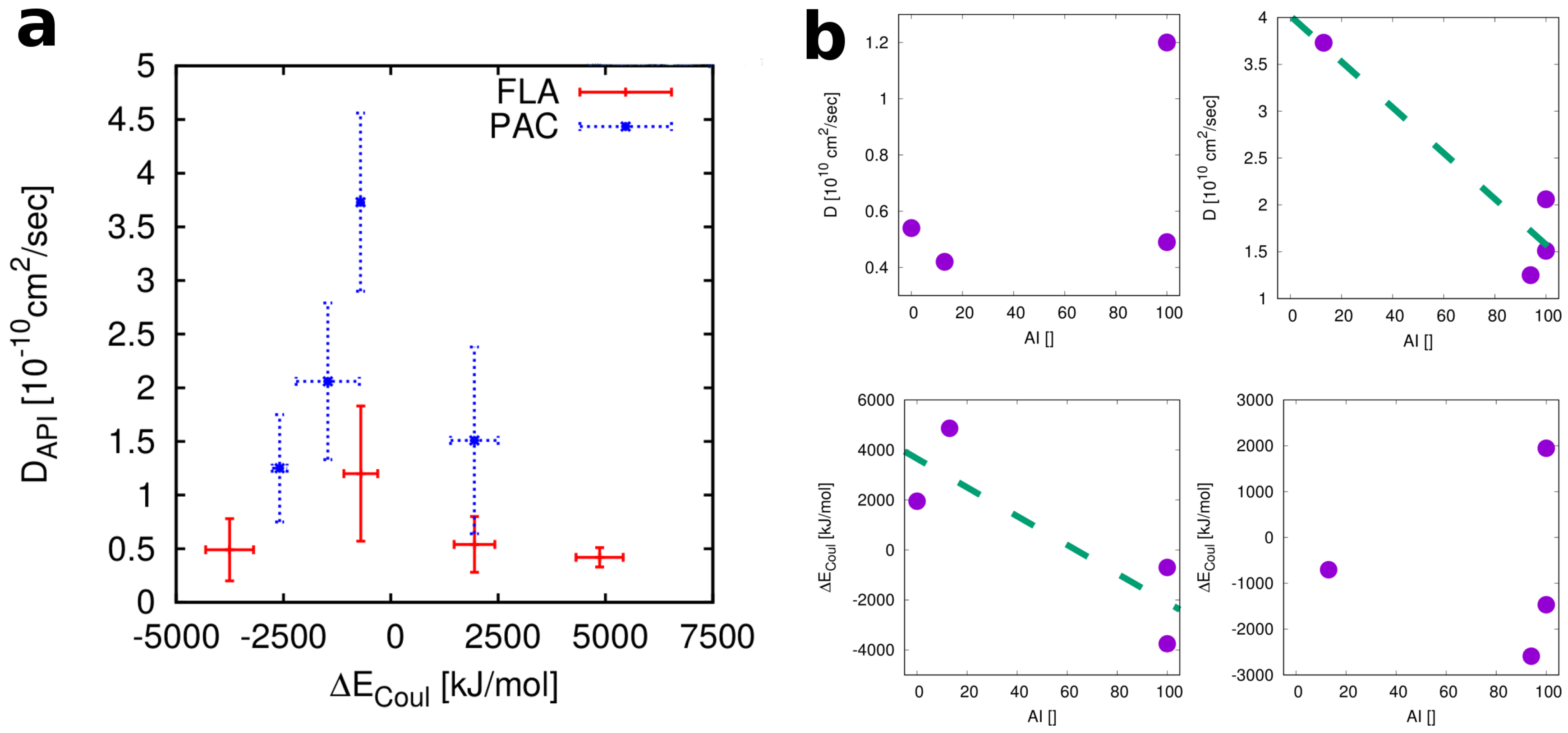
4. Discussion
4.1. Thermodynamics vs. Kinetics
4.2. Relevant Properties of API and Excipient
4.3. Some Technical Considerations
4.4. What Are Practical Implications?
5. Summary and Conclusions
Supplementary Materials
Author Contributions
Funding
Conflicts of Interest
Abbreviations
| API | Active Pharmaceutical Ingredient |
| ASD | Amorphous Solid Dispersions |
| PVP | Polyvinylpyrrolidone |
| HPMC | Hydroxypropyl Methylcellulose |
| DSC | Differential Scanning Calorimetry |
| MD | Molecular Dynamics |
| FH | Flory–Huggins |
| FLA | Flufenamic acid |
| PAC | Phenacetin |
| EEC | Eudragit E100 |
| PAA | Polyacrylic acid |
| PSA | Poly (styrene sulfonic acid) |
| GAFF | General Amber Force Field |
| RESP | Restrained Electrostatic Potential |
| GROMACS | Groningen Machine for Chemical Simulations |
| LINCS | Linear Constraint Solver |
| PME | Particle Mesh Ewald |
| AI | Amorphocity Indices |
| VdW | Van der Waals |
| E | change in Coloumb energy |
| NHB | change in number of H-bonds |
| RMSF | average root mean square fluctuation |
| D | Diffusion coefficient |
| RT | Room Temperature |
| GPU | Graphic Processing Unit |
References
- Williams, H.D.; Trevaskis, N.L.; Charman, S.A.; Shanker, R.M.; Charman, W.N.; Pouton, C.W.; Porter, C.J.H. Strategies to Address Low Drug Solubility in Discovery and Development. Pharmacol. Rev. 2013, 65, 315–499. [Google Scholar] [CrossRef] [PubMed]
- Baghel, S.; Cathcart, H.; O’Reilly, N.J. Polymeric Amorphous Solid Dispersions: A Review of Amorphization, Crystallization, Stabilization, Solid-State Characterization, and Aqueous Solubilization of Biopharmaceutical Classification System Class II Drugs. J. Pharm. Sci. 2016, 105, 2527–2544. [Google Scholar] [CrossRef] [PubMed]
- Sareen, S.; Joseph, L.; Mathew, G. Improvement in Solubility of Poor Water-Soluble Drugs by Solid Dispersion. Int. J. Pharm. Investig. 2012, 2, 12–17. [Google Scholar] [CrossRef] [PubMed]
- Newman, A. (Ed.) Pharmaceutical Amorphous Solid Dispersions; John Wiley & Sons, Inc.: Hoboken, NJ, USA, 2015. [Google Scholar]
- Dengale, S.J.; Grohganz, H.; Rades, T.; Löbmann, K. Recent Advances in Co-Amorphous Drug Formulations. Adv. Drug Deliv. Rev. 2015, 100, 116–125. [Google Scholar] [CrossRef] [PubMed]
- Tao, J.; Sun, Y.; Zhang, G.G.Z.; Yu, L. Solubility of Small-Molecule Crystals in Polymers: D-Mannitol in PVP, Indomethacin in PVP/VA, and Nifedipine in PVP/VA. Pharm. Res. 2009, 26, 855–864. [Google Scholar] [CrossRef] [PubMed]
- Qian, F.; Huang, J.; Hussain, M.A. Drug-Polymer Solubility and Miscibility: Stability Consideration and Practical Challenges in Amorphous Solid Dispersion Development. J. Pharm. Sci. 2010, 99, 2941–2947. [Google Scholar] [CrossRef] [PubMed]
- Liu, L.; Gronenborn, A.; Bahar, I. Longer Simulations Sample Larger Subspaces of Conformations while Maintaining Robust Mechanisms of Motion. Proteins Struct. Funct. Bioinform. 2012, 80, 616–625. [Google Scholar] [CrossRef] [PubMed]
- Knopp, M.M.; Gannon, N.; Porsch, I.; Rask, M.B.; Olesen, N.E.; Langguth, P.; Holm, R.; Rades, T. A Promising New Method to Estimate Drug-Polymer Solubility at Room Temperature. J. Pharm. Sci. 2016, 105, 2621–2624. [Google Scholar] [CrossRef] [PubMed]
- Paudel, A.; Van Humbeeck, J.; Van den Mooter, G. Theoretical and Experimental Investigation on the Solid Solubility and Miscibility of Naproxen in Poly(vinylpyrrolidone). Mol. Pharm. 2010, 7, 1133–1148. [Google Scholar] [CrossRef] [PubMed]
- Knopp, M.M.; Olesen, N.E.; Holm, P.; Langguth, P.; Holm, R.; Rades, T. Influence of Polymer Molecular Weight on Drug-Polymer Solubility: A Comparison between Experimentally Determined Solubility in PVP and Prediction Derived from Solubility in Monomer. J. Pharm. Sci. 2015, 104, 2905–2912. [Google Scholar] [CrossRef] [PubMed]
- Knopp, M.M.; Tajber, L.; Tian, Y.; Olesen, N.E.; Jones, D.S.; Kozyra, A.; Loebmann, K.; Paluch, K.; Brennan, C.M.; Holm, R.; et al. A Comparative Study of Different Methods for the Prediction of Drug-Polymer Solubility. Mol. Pharm. 2015, 12, 3408–3419. [Google Scholar] [CrossRef] [PubMed]
- Tetko, I.V.; Gasteiger, J.; Todeschini, R.; Mauri, A.; Livingstone, D.; Ertl, P.; Palyulin, V.A.; Radchenko, E.V.; Zefirov, N.S.; Makarenko, A.S.; et al. Virtual Computational Chemistry Laboratory–Design and Description. J. Comput.-Aided Mol. Des. 2005, 19, 453–463. [Google Scholar] [CrossRef] [PubMed]
- Moore, M.D.; Wildfong, P.L.D. Informatics Calibration of a Molecular Descriptors Database to Predict Solid Dispersion Potential of Small Molecule Organic Solids. Int. J. Pharm. 2011, 418, 217–226. [Google Scholar] [CrossRef] [PubMed]
- Nurzyńska, K.; Booth, J.; Roberts, C.J.; McCabe, J.; Dryden, I.; Fischer, P.M. Long-Term Amorphous Drug Stability Predictions Using Easily Calculated, Predicted, and Measured Parameters. Mol. Pharm. 2015, 12, 3389–3398. [Google Scholar] [CrossRef] [PubMed]
- Huggins, M.M.L. Thermodynamic Properties of Solutions of Long-Chain Compounds. Ann. N. Y. Acad. Sci. 1942, 43, 1–32. [Google Scholar] [CrossRef]
- Flory, P.J. Thermodynamics of High Polymer Solutions. J. Chem. Phys. 1942, 10, 51–61. [Google Scholar] [CrossRef]
- Marsac, P.J.; Shamblin, S.L.; Taylor, L.S. Theoretical and Practical Approaches for Prediction of Drug-Polymer Miscibility and Solubility. Pharm. Res. 2006, 23, 2417–2426. [Google Scholar] [CrossRef] [PubMed]
- Yoo, S.u.; Krill, S.; Wang, Z.; Telang, C. Miscibility/stability Considerations in Binary Solid Dispersion Systems Composed of Functional Excipients towards the Design of Multi-Component Amorphous Systems. J. Pharm. Sci. 2009, 98, 4711–4723. [Google Scholar] [CrossRef] [PubMed]
- Tian, Y.; Booth, J.; Meehan, E.; Jones, D.S.; Li, S.; Andrews, G.P. Construction of Drug-Polymer Thermodynamic Phase Diagrams Using Flory–Huggins Interaction Theory: Identifying the Relevance of Temperature and Drug Weight Fraction to Phase Separation within Solid Dispersions. Mol. Pharm. 2013, 10, 236–248. [Google Scholar] [CrossRef] [PubMed]
- Thakral, S.; Thakral, N.K.N. Prediction of Drug-Polymer Miscibility through the Use of Solubility Parameter Based Flory–Huggins Interaction Parameter and the Experimental Validation: PEG as Model Polymer. J. Pharm. Sci. 2013, 102, 2254–2263. [Google Scholar] [CrossRef] [PubMed]
- Van der Waals, J.H. Flory–Huggins Lattice Model Theory on Defensive. Chem. Eng. News 1951, 29, 3959–3961. [Google Scholar]
- Kestur, U.S.; Van Eerdenbrugh, B.; Taylor, L.S. Influence of Polymer Chemistry on Crystal Growth Inhibition of Two Chemically Diverse Organic Molecules. CrystEngComm 2011, 13, 6712–6718. [Google Scholar] [CrossRef]
- Habgood, M.; Lancaster, R.W.; Gateshki, M.; Kenwright, A.M. The Amorphous Form of Salicylsalicylic Acid: Experimental Characterization and Computational Predictability. Cryst. Growth Des. 2013, 13, 1771–1779. [Google Scholar] [CrossRef]
- Wegiel, L.a.; Mauer, L.J.; Edgar, K.J.; Taylor, L.S. Mid-Infrared Spectroscopy as a Polymer Selection Tool for Formulating Amorphous Solid Dispersions. J. Pharm. Pharmacol. 2014, 66, 244–255. [Google Scholar] [CrossRef] [PubMed]
- Gross, J.; Sadowski, G. Perturbed-Chain SAFT: An Equation of State Based on a Perturbation Theory for Chain Molecules. Ind. Eng. Chem. Res. 2001, 40, 1244–1260. [Google Scholar] [CrossRef]
- Paus, R.; Ji, Y.; Vahle, L.; Sadowski, G. Predicting the Solubility Advantage of Amorphous Pharmaceuticals: A Novel Thermodynamic Approach. Mol. Pharm. 2015, 12, 2823–2833. [Google Scholar] [CrossRef] [PubMed]
- Gupta, P.; Thilagavathi, R.; Chakraborti, A.K.; Bansal, A.K. Role of Molecular Interaction in Stability of Celecoxib-PVP Amorphous Systems. Mol. Pharm. 2005, 2, 384–391. [Google Scholar] [CrossRef] [PubMed]
- Xiang, T.X.; Anderson, B.D. Molecular Dynamics Simulation of Amorphous Indomethacin-Poly (vinylpyrrolidone) Glasses: Solubility and Hydrogen Bonding Interactions. J. Pharm. Sci. 2013, 102, 876–891. [Google Scholar] [CrossRef] [PubMed]
- Jha, P.K.; Larson, R.G. Assessing the Efficiency of Polymeric Excipients by Atomistic Molecular Dynamics Simulations. Mol. Pharm. 2014, 11, 1676–1686. [Google Scholar] [CrossRef] [PubMed]
- Maniruzzaman, M.; Pang, J.; Morgan, D.J.; Douroumis, D. Molecular Modeling as a Predictive Tool for the Development of Solid Dispersions. Mol. Pharm. 2015, 12, 1040–1049. [Google Scholar] [CrossRef] [PubMed]
- Gupta, J.; Nunes, C.; Vyas, S.; Jonnalagadda, S. Prediction of Solubility Parameters and Miscibility of Pharmaceutical Compounds by Molecular Dynamics Simulations. J. Phys. Chem. B 2011, 115, 2014–2023. [Google Scholar] [CrossRef] [PubMed]
- Kawakami, K.; Pikal, M.J. Calorimetric Investigation of the Structural Relaxation of Amorphous Materials: Evaluating Validity of the Methodologies. J. Pharm. Sci. 2005, 94, 948–965. [Google Scholar] [CrossRef] [PubMed]
- Bhugra, C.; Pikal, M. Role of Thermodynamic, Molecular, and Kinetic Factors in Crystallization from the Amorphous State. J. Pharm. Sci. 2008, 97, 1329–1349. [Google Scholar] [CrossRef] [PubMed]
- Bhattacharya, S.; Suryanarayanan, R. Local Mobility in Amorphous Pharmaceuticals—Characterization and Implications on Stability. J. Pharm. Sci. 2009, 98, 2935–2953. [Google Scholar] [CrossRef] [PubMed]
- Kothari, K.; Ragoonanan, V.; Suryanarayanan, R. Influence of Molecular Mobility on the Physical Stability of Amorphous Pharmaceuticals in the Supercooled and Glassy States. Mol. Pharm. 2014, 11, 3048–3055. [Google Scholar] [CrossRef] [PubMed]
- Knapik, J.; Wojnarowska, Z.; Grzybowska, K.; Jurkiewicz, K.; Tajber, L.; Paluch, M. Molecular Dynamics and Physical Stability of Coamorphous Ezetimib and Indapamide Mixtures. Mol. Pharm. 2015, 12, 3610–3619. [Google Scholar] [CrossRef] [PubMed]
- Yalkowsky, S.H.; He, Y.; Jain, P. Handbook of Aqueous Solubility Data; CRC Press Taylor & Francis Group: Boca Raton, FL, USA, 2010; p. 1608. [Google Scholar]
- Wang, J.; Wolf, R.M.; Caldwell, J.W.; Kollman, P.A.; Case, D.A. Development and Testing of a General Amber Force Field. J. Comput. Chem. 2004, 25, 1157–1174. [Google Scholar] [CrossRef] [PubMed]
- Case, D.A.; Darden, T.A.; Cheatham, T.E.; Simmerling, C.; Wang, J.; Duke, R.; Luo, R.; Walker, R.; Zhang, W.; Merz, K.; et al. Amber16. 2016. Available online: http://ambermd.org (accessed on June 2016).
- Sousa da Silva, A.W.; Vranken, W.F. ACPYPE-AnteChamber PYthon Parser Interfac. BMC Res. Notes 2012, 5, 367. [Google Scholar] [CrossRef] [PubMed]
- Mobley, D.L.; Chodera, J.D.; Dill, K.A. On the Use of Orientational Restraints and Symmetry Corrections in Alchemical Free Energy Calculations. J. Chem. Phys. 2006, 125, 084902. [Google Scholar] [CrossRef] [PubMed]
- Xiang, T.X.; Anderson, B.D. A Molecular Dynamics Simulation of Reactant Mobility in an Amorphous Formulation of a Peptide in Poly(vinylpyrrolidone). J. Pharm. Sci. 2004, 93, 855–876. [Google Scholar] [CrossRef] [PubMed]
- Vanquelef, E.; Simon, S.; Marquant, G.; Garcia, E.; Klimerak, G.; Delepine, J.C.; Cieplak, P.; Dupradeau, F.Y. RED Server: A Web Service for Deriving RESP and ESP Charges and Building Force Field Libraries for New Molecules and Molecular Fragments. Nucleic Acids Res. 2011, 39, W511–W517. [Google Scholar] [CrossRef] [PubMed]
- Gordon, M.S.; Schmidt, M.W. Chapter 41—Advances in Electronic Structure Theory: GAMESS a Decade Later. In Theory and Applications of Computational Chemistry; Dykstra, C.E., Frenking, G., Kim, K.S., Scuseria, G.E., Eds.; Elsevier: New York, NY, USA, 2005; pp. 1167–1189. [Google Scholar]
- Pronk, S.; Páll, S.; Schulz, R.; Larsson, P.; Bjelkmar, P.; Apostolov, R.; Shirts, M.R.; Smith, J.C.; Kasson, P.M.; van der Spoel, D.; et al. GROMACS 4.5: A High-Throughput and Highly Parallel Open Source Molecular Simulation Toolkit. Bioinformatics 2013, 29, 845–854. [Google Scholar] [CrossRef] [PubMed]
- Hoover, W.G. Canonical Dynamics: Equilibrium Phase-Space Distributions. Phys. Rev. A 1985, 31, 1695–1697. [Google Scholar] [CrossRef]
- Berendsen, H.J.C.; Postma, J.P.M.; van Gunsteren, W.F.; DiNola, A.; Haak, J.R. Molecular Dynamics with Coupling to an External Bath. J. Chem. Phys. 1984, 81, 3684–3690. [Google Scholar] [CrossRef]
- Essmann, U.; Perera, L.; Berkowitz, M.L.; Darden, T.; Lee, H.; Pedersen, L.G. A Smooth Particle Mesh Ewald Potential. J. Chem. Phys. 1995, 103, 8577–8592. [Google Scholar] [CrossRef]
- Hess, B.; Bekker, H.; Berendsen, H.J.C.; Fraaije, J.G.E.M. LINCS: A Linear Constraint Solver for Molecular Simulations. J. Comput. Chem. 1997, 18, 1463–1472. [Google Scholar] [CrossRef]
- Eerdenbrugh, B.V.; Taylor, L. Small Scale Screening to Determine the Ability of Different Polymers to Inhibit Drug Crystallization upon Rapid Solvent Evaporation. Mol. Pharm. 2010, 7, 1328–1337. [Google Scholar] [CrossRef] [PubMed]
- Fadda, E.; Woods, R.J. Molecular Simulations of Carbohydrates and Protein-Carbohydrate Interactions: Motivation, Issues and Prospects. Drug Discov. Today 2010, 15, 596–609. [Google Scholar] [CrossRef] [PubMed]
- Matthews, J.F.; Beckham, G.T.; Bergenstråhle-Wohlert, M.; Brady, J.W.; Himmel, M.E.; Crowley, M.F. Comparison of Cellulose Iβ Simulations with Three Carbohydrate Force Fields. J. Chem. Theory Comput. 2012, 8, 735–748. [Google Scholar] [CrossRef] [PubMed]
- Xiang, T.X.; Anderson, B.D. Distribution and Effect of Water Content on Molecular Mobility in Poly(vinylpyrrolidone) Glasses: A Molecular Dynamics Simulation. Pharm. Res. 2005, 22, 1205–1214. [Google Scholar] [CrossRef] [PubMed]
- Wegiel, L.a.; Zhao, Y.; Mauer, L.J.; Edgar, K.J.; Taylor, L.S. Curcumin Amorphous Solid Dispersions: The Influence of Intra and Intermolecular Bonding on Physical Stability. Pharm. Dev. Technol. 2014, 19, 976–986. [Google Scholar] [CrossRef] [PubMed]
- Hancock, B.C.; Shamblin, S.L.; Zografi, G. Molecular Mobility of Amorphous Pharmaceutical Solids below their Glass Transition Temperatures. Pharm. Res. 1995, 12, 799–806. [Google Scholar] [CrossRef] [PubMed]
- Ozal, T.A.; Peter, C.; Hess, B.; van der Vegt, N.F.A. Modeling Solubilities of Additives in Polymer Microstructures: Single-Step Perturbation Method Based on a Soft-Cavity Reference State. Macromolecules 2008, 41, 5055–5061. [Google Scholar] [CrossRef]
- Hess, B.; Peter, C.; Ozal, T.; van der Vegt, N.F. Fast-Growth Thermodynamic Integration: Calculating Excess Chemical Potentials of Additive Molecules in Polymer Microstructures. Macromolecules 2008, 41, 2283–2289. [Google Scholar] [CrossRef]
- Rosenfeld, Y. A Quasi-Universal Scaling Law for Atomic Transport in Simple Fluids. J. Phys. Condens. Matter 1999, 11, 5415–5427. [Google Scholar] [CrossRef]
- Dzugutov, M. A Universal Scaling Law for Atomic Diffusion in Condensed Matter. Nature 1996, 381, 137–139. [Google Scholar] [CrossRef]
- Xiang, T.X.; Anderson, B.D. Molecular dynamics simulation of amorphous hydroxypropyl-methylcellulose acetate succinate (HPMCAS): Polymer model development, water distribution, and plasticization. Mol. Pharm. 2014, 11, 2400–2411. [Google Scholar] [CrossRef] [PubMed]
- Xiang, T.X.; Anderson, B.D. Molecular Dynamics Simulation of Amorphous Hydroxypropylmethylcellulose and Its Mixtures with Felodipine and Water. J. Pharm. Sci. 2017, 106, 803–816. [Google Scholar] [CrossRef] [PubMed]
- Shimpi, S.L.; Mahadik, K.R.; Paradkar, A.R. Study on Mechanism for Amorphous Drug Stabilization Using Gelucire 50/13. Chem. Pharm. 2009, 57, 937–942. [Google Scholar] [CrossRef]
- Harvey, J.A.; Auerbach, S.M. Simulating Hydrogen-Bond Structure and Dynamics in Glassy Solids Composed of Imidazole Oligomers. J. Phys. Chem. B 2014, 118, 7609–7617. [Google Scholar] [CrossRef] [PubMed]
- Lindert, S.; Bucher, D.; Eastman, P.; Pande, V.; Mccammon, J.A. Accelerated Molecular Dynamics Simulations with the AMOEBa Polarizable Force Field on Graphics Processing Units. J. Chem. Theory Comput. 2013, 9, 4684–4691. [Google Scholar] [CrossRef] [PubMed]
- Eastman, P.; Friedrichs, M.S.; Chodera, J.D.; Radmer, R.J.; Bruns, C.M.; Ku, J.P.; Beauchamp, K.A.; Lane, T.J.; Wang, L.P.; Shukla, D.; et al. OpenMM 4: A Reusable, Extensible, Hardware Independent Library for High Performance Molecular Simulation. J. Chem. Theory Comput. 2013, 9, 461–469. [Google Scholar] [CrossRef] [PubMed]
- Arthur, E.J.; Brooks, C.L. Efficient Implementation of Constant PH Molecular Dynamics on Modern Graphics Processors. J. Comput. Chem. 2016, 37, 2171–2180. [Google Scholar] [CrossRef] [PubMed]


| Polymer | N a | N b | API | N c | m d | w(API) e | V f |
|---|---|---|---|---|---|---|---|
| EEC | 14 | 40 | FLA | 95 | 108,631 | 24.6 | 161.0 |
| PAA | 28 | 40 | FLA | 95 | 107,486 | 24.9 | 133.8 |
| PSA | 12 | 40 | FLA | 95 | 99,774 | 23.2 | 139.2 |
| PVP | 18 | 40 | FLA | 95 | 106,778 | 25.0 | 152.0 |
| EEC | 14 | 40 | FLA | 190 | 135,348 | 39.5 | 193.5 |
| PAA | 28 | 40 | FLA | 190 | 134,203 | 39.8 | 166.5 |
| PSA | 12 | 40 | FLA | 190 | 126,491 | 37.7 | 171.4 |
| PVP | 18 | 40 | FLA | 190 | 133,495 | 40.0 | 184.1 |
| EEC | 14 | 40 | PAC | 149 | 108,617 | 24.6 | 167.5 |
| PAA | 28 | 40 | PAC | 149 | 107,472 | 24.8 | 140.2 |
| PSA | 12 | 40 | PAC | 149 | 99,761 | 23.2 | 144.9 |
| PVP | 18 | 40 | PAC | 149 | 106,764 | 25.0 | 157.0 |
| EEC | 14 | 40 | PAC | 298 | 135,321 | 39.5 | 206.3 |
| PAA | 28 | 40 | PAC | 298 | 134,176 | 39.8 | 179.5 |
| PSA | 12 | 40 | PAC | 298 | 126,464 | 37.6 | 183.6 |
| PVP | 18 | 40 | PAC | 298 | 133,468 | 40.0 | 195.7 |
| EEC | 14 | 40 | – | – | 81,913 | 0 | 128.7 |
| PAA | 28 | 40 | – | – | 80,769 | 0 | 100.2 |
| PSA | 12 | 40 | – | – | 88,446 | 0 | 107.3 |
| PVP | 18 | 40 | – | – | 80,061 | 0 | 120.1 |
| – | – | – | FLA | 302 | 84,933 | 100.0 | 104.9 |
| – | – | – | PAC | 475 | 85,130 | 100.0 | 128.0 |
| API | Polymer | AI25 a | AI40 b | <AI> c | Ed | D e | RMSF f |
|---|---|---|---|---|---|---|---|
| FLA | EEC | 100 | 100 | 87 | −698.7 | 1.20 | 0.082 |
| FLA | PAA | 25 | 13 | 13 | 4863.8 | 0.42 | 0.068 |
| FLA | PSA | 0 | 0 | 15 | 1948.8 | 0.54 | 0.078 |
| FLA | PVP | 100 | 100 | 87 | −3753.7 | 0.49 | 0.080 |
| PAC | EEC | 25 | 13 | 13 | −704.0 | 3.73 | 0.0892 |
| PAC | PAA | 100 | 100 | 67 | 1945.4 | 1.51 | 0.0724 |
| PAC | PSA | 100 | 100 | 78 | −1468.4 | 2.06 | 0.0790 |
| PAC | PVP | 100 | 94 | 49 | −2590.1 | 1.25 | 0.0721 |
© 2018 by the authors. Licensee MDPI, Basel, Switzerland. This article is an open access article distributed under the terms and conditions of the Creative Commons Attribution (CC BY) license (http://creativecommons.org/licenses/by/4.0/).
Share and Cite
Brunsteiner, M.; Khinast, J.; Paudel, A. Relative Contributions of Solubility and Mobility to the Stability of Amorphous Solid Dispersions of Poorly Soluble Drugs: A Molecular Dynamics Simulation Study. Pharmaceutics 2018, 10, 101. https://doi.org/10.3390/pharmaceutics10030101
Brunsteiner M, Khinast J, Paudel A. Relative Contributions of Solubility and Mobility to the Stability of Amorphous Solid Dispersions of Poorly Soluble Drugs: A Molecular Dynamics Simulation Study. Pharmaceutics. 2018; 10(3):101. https://doi.org/10.3390/pharmaceutics10030101
Chicago/Turabian StyleBrunsteiner, Michael, Johannes Khinast, and Amrit Paudel. 2018. "Relative Contributions of Solubility and Mobility to the Stability of Amorphous Solid Dispersions of Poorly Soluble Drugs: A Molecular Dynamics Simulation Study" Pharmaceutics 10, no. 3: 101. https://doi.org/10.3390/pharmaceutics10030101
APA StyleBrunsteiner, M., Khinast, J., & Paudel, A. (2018). Relative Contributions of Solubility and Mobility to the Stability of Amorphous Solid Dispersions of Poorly Soluble Drugs: A Molecular Dynamics Simulation Study. Pharmaceutics, 10(3), 101. https://doi.org/10.3390/pharmaceutics10030101