A Guide to In Silico Drug Design

Abstract

The drug discovery process is a rocky path that is full of challenges, with the result that very few candidates progress from hit compound to a commercially available product, often due to factors, such as poor binding affinity, off-target effects, or physicochemical properties, such as solubility or stability. This process is further complicated by high research and development costs and time requirements. It is thus important to optimise every step of the process in order to maximise the chances of success. As a result of the recent advancements in computer power and technology, computer-aided drug design (CADD) has become an integral part of modern drug discovery to guide and accelerate the process. In this review, we present an overview of the important CADD methods and applications, such as in silico structure prediction, refinement, modelling and target validation, that are commonly used in this area.

1. Introduction

New drugs with better efficacy and reduced toxicity are always in high demand, however the process of drug discovery and development is costly and time consuming and presents a number of challenges. The pitfalls of target validation and hit identification aside, a high failure rate is often observed in clinical trials due to poor pharmacokinetics, poor efficacy, and high toxicity [1,2]. A study conducted by Wong et al. that analysed 406,038 trials from January 2000 to October 2015 showed that the probability of success for all drugs (marketed and in development) was only 13.8% [3]. In 2016, DiMasi and colleagues [4] estimated a research and development (R&D) cost for a new drug of USD $2.8 billion based upon data for 106 randomly selected new drugs developed by 10 pharmaceutical companies. The average time taken from synthesis to first human testing was estimated to be approximately 2.6 years (31.2 months) and cost approximately USD $430 million, and from the start of a clinical testing to submission with the FDA was 6 to 7 years (80.8 months). In comparison to a study conducted by the same author in 2003, the R&D cost for a new drug had increased drastically by more than two-fold (from USD $1.2 billion) [5]. A possible reason for the increase in R&D cost is that regulators, such as the FDA have become more risk averse, tightening safety requirements, leading to higher failure rates in trials and increased costs for drug development. It is therefore important to optimise every aspect of the R&D process in order to maximise the chances of success.

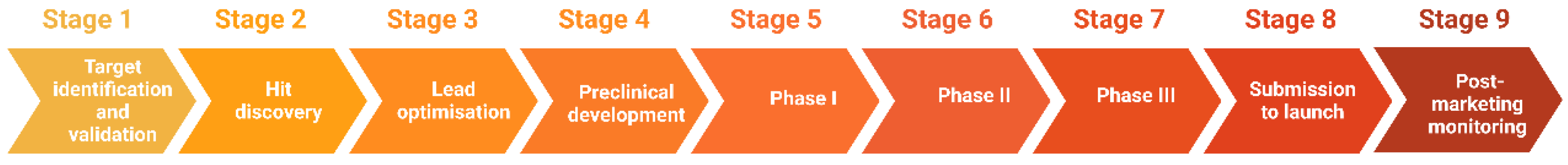
The process of drug discovery starts with target identification, followed by target validation, hit discovery, lead optimisation, and preclinical/clinical development. If successful, a drug candidate progresses to the development stage, where it passes through different phases of clinical trials and eventually submission for approval to launch on the market (Figure 1) [6].

Briefly, drug targets can be identified using methods, such as data-mining [7], phenotype screening [8,9], and bioinformatics (e.g., epigenetic, genomic, transcriptomic, and proteomic methods) [10]. Potential targets must then be validated to determine whether they are rate limiting for the disease’s progression or induction. Establishing a strong link between the target and disease builds up confidence in the scientific hypothesis and thus greater success and efficiency in later stages of the drug discovery process [11,12].

Once the targets are identified and validated, compound screening assays are carried out to discover novel hit compounds (hit-to-lead). There are various strategies that can be used in this screening, involving physical methods, such as mass spectrometry [13], fragment screening [14,15], nuclear magnetic resonance (NMR) screening [16], DNA encoded chemical libraries [17], high throughput screening (HTS) (such as protein or cells) [18] or in silico methods, such as virtual screening (VS) [19].

After hit compounds are identified, properties, such as absorption, distribution, metabolism, excretion (ADME), and toxicity should be considered and optimised early in the drug discovery process. Unfavourable pharmacokinetic and toxicity profile of a drug candidate is one of the hurdles that often leads to failure in the clinical trials [20].

Although physical and computational screening techniques are distinct in nature, they are often integrated in the drug discovery process to complement each other and maximise the potential of the screening results [21].

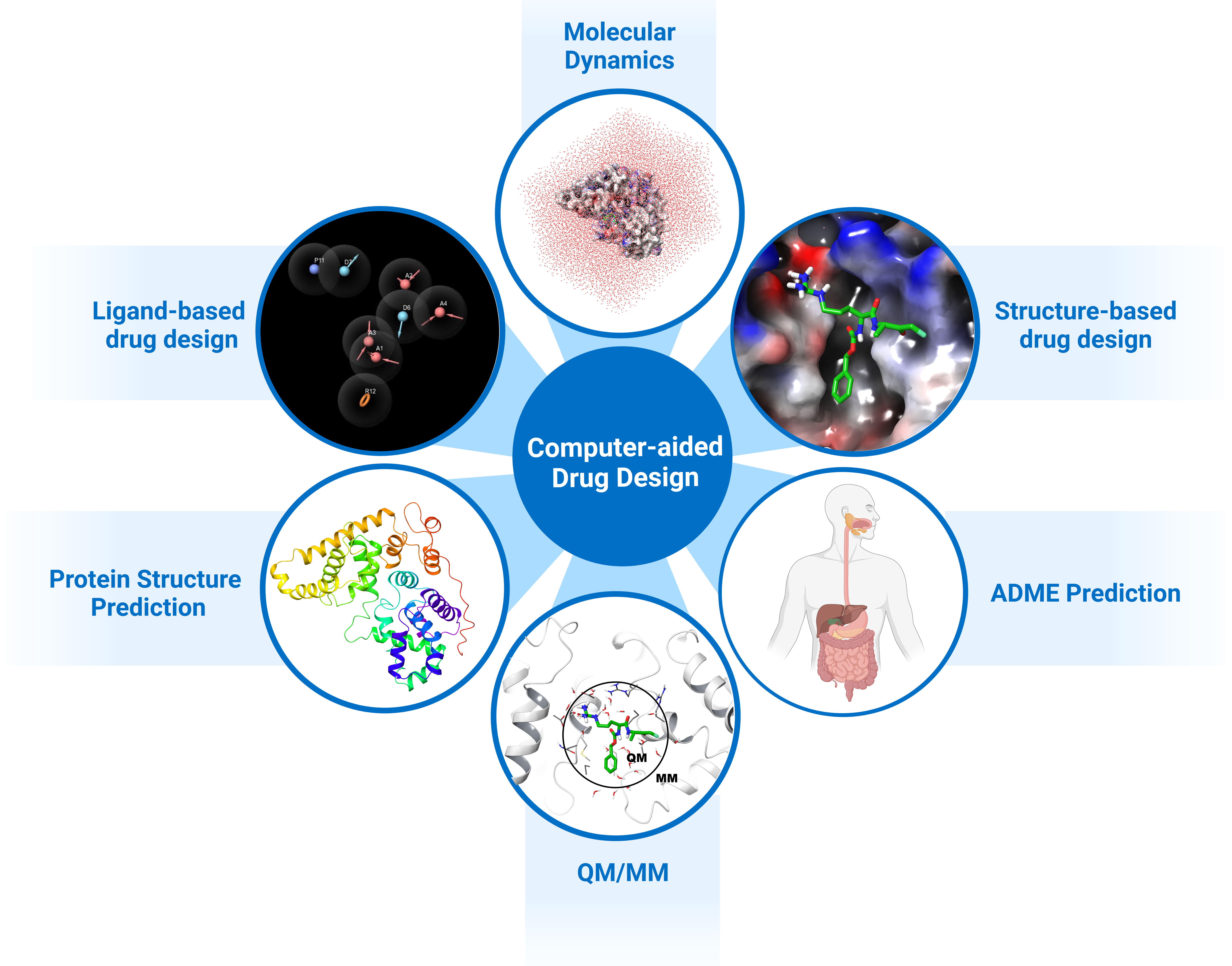
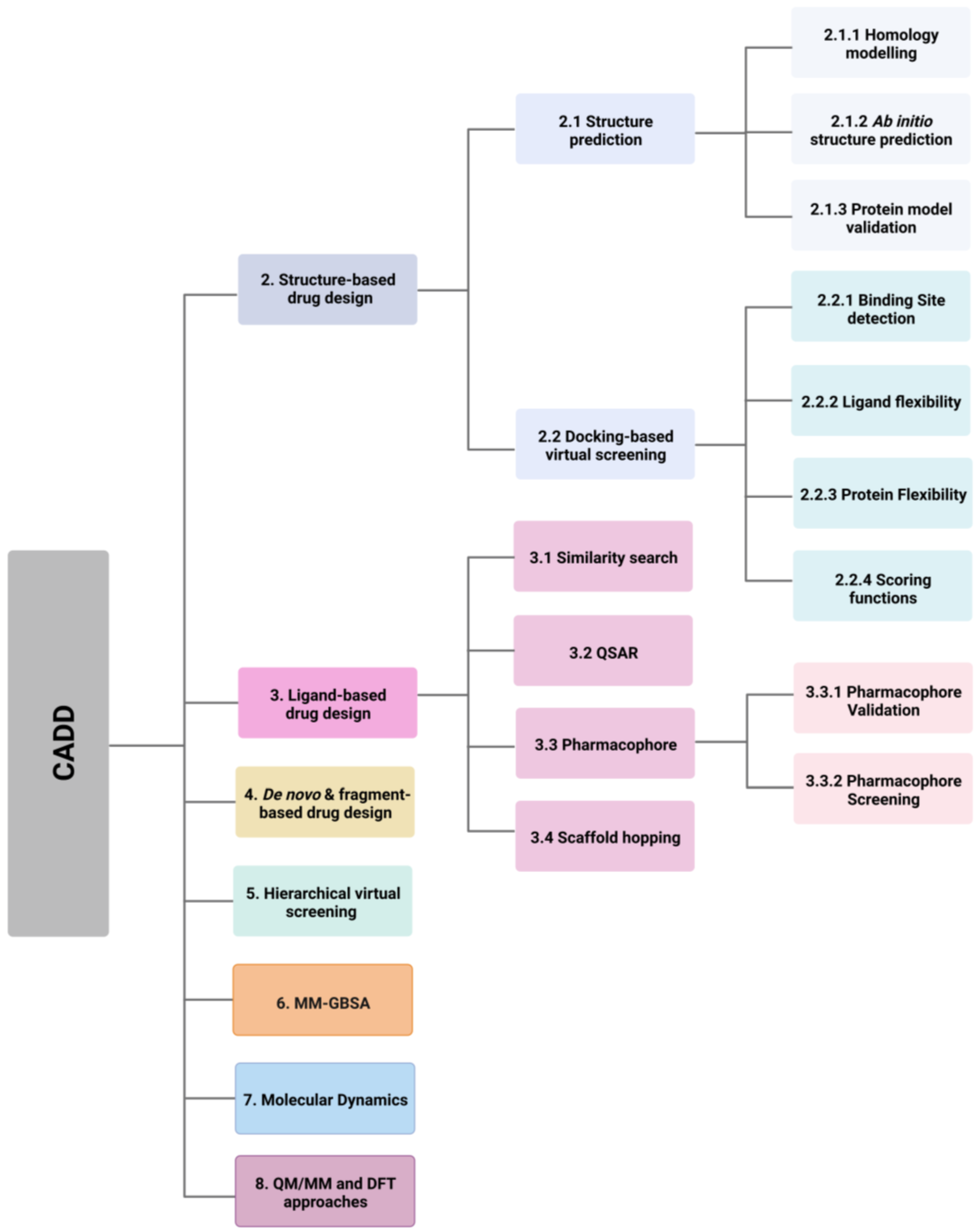
Computer-aided drug design (CADD) utilises this information and knowledge to screen for novel drug candidates. With the advancement in technology and computer power in recent years, CADD has proven to be a tool that reduces the time and resources required in the drug discovery pipeline. The aim of this review is to give an overview of the various in silico techniques that are used in the drug discovery process (Figure 2).

2. Structure-Based Drug Design

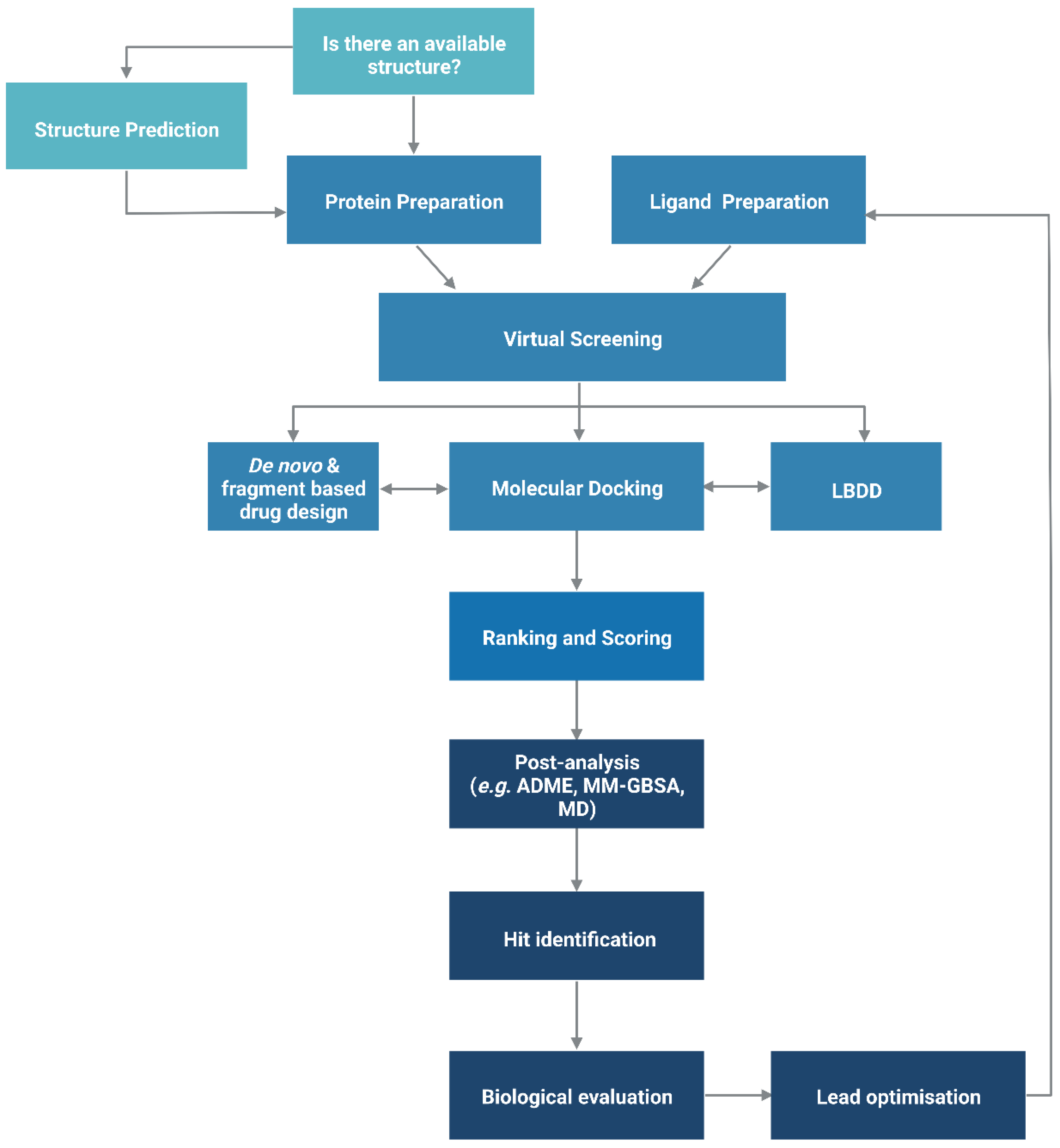
The functionality of a protein is dependent upon its structure, and structure-based drug design (SBDD) relies on the 3D structural information of the target protein, which can be acquired from experimental methods, such as X-ray crystallography, NMR spectroscopy and cryo-electron microscopy (cryo-EM). The aim of SBDD is to predict the Gibbs free energy of binding (ΔG_bind), the binding affinity of ligands to the binding site, by simulating the interactions between them. Some examples of SBDD include molecular dynamics (MD) simulations [22], molecular docking [23], fragment-based docking [24], and de novo drug design [25]. Figure 3 describes a general workflow of molecular docking that will be discussed in greater detail.

2.1. Protein Structure Prediction

The advancements in sequencing technology led to a steep increase in recorded genetic information thus rapidly widening the gap between the amounts of sequence and structural data available. As of May 2022, the UniprotKB/TrEMBL database contained over 231 million sequence entries, yet there are only approximate 193,000 structures recorded in the Protein Data Bank (PDB) [26,27]. To model the structures of those proteins where structural data is not available, homology (comparative) modelling or ab initio methods can be used.

2.1.1. Homology Modelling

Homology modelling involves predicting the structure of a protein by aligning its sequence to a homologous protein that serves as a template for the construction of the model. The process can be broken down into three steps: (1) template identification, (2) sequence-template alignment, and (3) model construction.

Firstly, the protein sequence is obtained, either experimentally or from databases, such as the Universal Protein Resource (UniProt) [28], and this is followed by identifying modelling templates that have high sequence similarity and resolution by performing a BLAST [29] search against the Protein Data Bank [30]. PSI-BLAST [29] uses profile-based methods to identify patterns of residue conservation, which can be more useful and accurate than simply comparing raw sequences, as protein functions are predominately determined by the structural arrangement rather than the amino acid sequence. One of the biggest limitations of homology modelling is that it relies heavily upon the availabilities of suitable templates and accurate sequence alignment. A high sequence identity between the query protein and the template normally gives greater confidence in the homology model. Generally, a minimum of 30% sequence identity is considered to be a threshold for successful homology modelling, as approximately 20% of the residues are expected to be misaligned for sequence identities below 30%, leading to poor homology models. Alignment errors are less frequent when the sequence identity is above 40%, where approximately 90% of the main-chain atoms are likely to be modelled with a root-mean-square deviation (RMSD) of ~1 Å, and the majority of the structural differences occur at loops and in side-chain orientations [31].

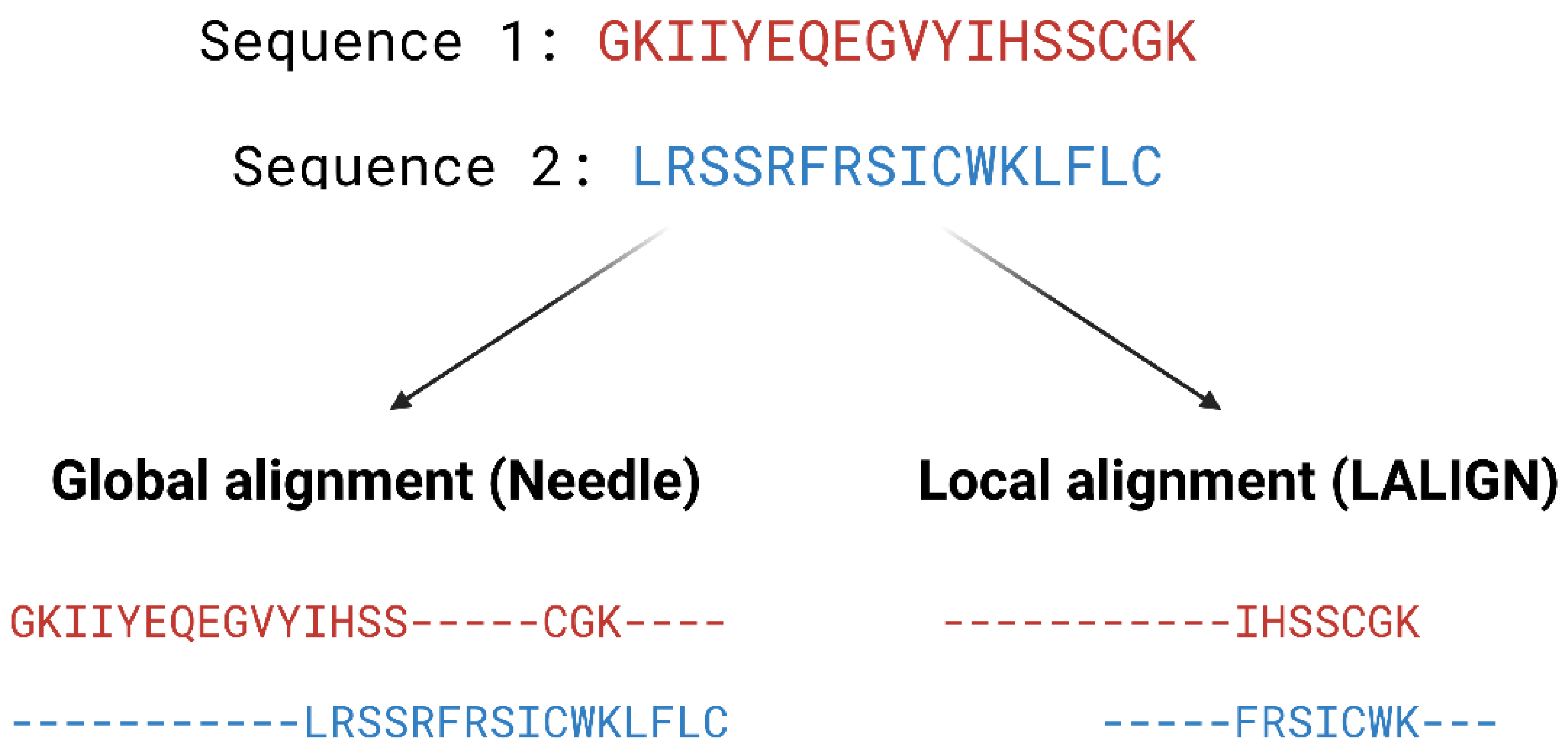
Pairwise alignment methods are used when comparing two sequences and they are generally divided into two categories—global and local alignment (Figure 4). Global alignment aims to align the entire sequences and are most useful when sequences are closely related or of similar lengths. Tools such as EMBOSS Needle [32] and EMBOSS Stretcher [32] use the Needleman–Wunsch algorithm [33] to perform global alignment. In comparison to using a somewhat brute-force approach, the Needleman–Wunsch algorithm uses dynamic programming to find the best alignment by reducing the number of possible alignments that need to be considered and guarantees to find the best alignment. Dynamic programming aims to break a larger problem (the entire sequence) into smaller problems which are then solved optimally. The solutions to these smaller problems are then used to construct an optimal solution to the original problem [34]. The Needleman–Wunsch algorithm first builds a matrix that is subjected to a gap penalty (negative scores in first row and column), and the matrix is used to assign a score to every possible alignment (usually positive score for match, no score or penalty for mismatch and gaps). Once the cells in the matrix are filled in, traceback starts from the lower right towards the top left of the matrix to find the best alignment with the highest score.

Local alignment, on the other hand, aims to identify regions that share high sequence similarity, which is more useful when aligning sequences that are dissimilar or distantly related. EMBOSS water [32] and LALIGN [32] are tools that use the Smith–Waterman algorithm [35] for local alignment. The Smith–Waterman algorithm, such as the Needleman-Wunsch algorithm, uses dynamic programming to perform sequence alignment. However, there is no negative score assigned in this algorithm, and the first row and column are set to 0. Traceback begins with the matrix cell from the highest score and travels up/left until it reaches 0 to produce the highest scoring local alignment.

When searching for templates used for homology modelling, including multiple sequences will improve accuracy of the alignment in regions where there is a low sequence homology, hence multiple sequence alignment (MSA) is essential. The global alignment method for multiple sequences is generally too computationally expensive; modern MSA tools (e.g., ClustalW [36], T-Coffee [37] and MUSCLE [38]) commonly use a progressive alignment approach that combines global and/or local alignment methods, followed by the branching order of a guide tree. This technique aims to achieve a succession of pairwise alignments, first aligning the most similar sequences and then progressing to the next most similar sequence until the entire query set has been incorporated.

For example, MSA was used during the construction of the homology models for Alanine-Serine-Cysteine transporter (SLC1A5) by Garibsingh et al. At the time, there was limited structural information on SLC1A5 due to the lack of an experimentally determined structure of human SCL1 family proteins. Most of the knowledge on the human SLC1 family protein therefore came from the study of prokaryotic homologs, which share low sequence identity. Using the structural information of the recently solved human SLC1A3, Garibsingh et al. carried out a phylogenetic analysis by generating MSA of the human SCL1 family and its prokaryotic homologs using MUSCLE and Promals3D [39], and built two different conformations of SLC1A5 homology models for the design of SLC1A5 inhibitors [40].

Once the alignment is complete, the model can be constructed starting with the backbone, then loops and lastly side-chains. The polypeptide backbone of the protein is first created by copying the coordinates of the residues from the template to create the model backbone. Gaps between the alignment of the sequence and the template are then taken care of through insertions and deletions in the alignment. It is important to remodel gaps accurately, as any error introduced here, will be amplified in later stages, thus leading to structural changes that can be critical for protein functionality and protein–protein interactions. Loop modelling, via knowledge-based methods or energy-based methods, can be used to generate predictions of the conformations of the loop. Knowledge-based methods look for experimental data on loops with high sequence similarity to the target from databases, such as PDB, and then insert them into the model. Yang et al. used FREAD [41] to predict the structure of a missing loop and construct a model of a monoclonal antibody, Se155-4, to study its antibody–antigen interactions with Salmonella Typhimurium O polysaccharide [42]. On the other hand, energy-based methods predict protein folding using ab initio methods with scoring function optimisation. For example, the Rosetta Next-Generation Kinematic Closure protocol [43], which employs the ab initio method, was used in loop prediction calculations to construct parts of the leucine-rich repeat kinase 2 (LRRK2) model, as the homology model template had missing loop sections. Mutations in the catalytic domains of LRRK2 are associated with familial and sporadic Parkinson’s disease, yet little is known about its overall structure and the mutations, which alter LRRK2 function and enzymatic activities. Combining homology models with experimental constraints, Guaitoli and co-workers constructed the first structural model of the full length LRRK2 that includes domain engagement and contacts. The model provided insight into the roles that the different domains play in the pathogenesis of Parkinson’s disease and will serve as a basis for future drug design on LRRK2 [44].

Lastly, side-chains are built onto the backbone model according to the target sequence. Most side-chain types in proteins have a limited number of conformations (rotamers) and programs such as SCWRL [45] predict these in order to minimise the total potential energy. Upon completion, the model is optimised using molecular mechanics force fields to improve its quality.

A ligand-based approach can be utilised to further optimise homology models with low sequence identity between query sequence and structural template. Moro et al. first presented ligand-based homology modelling, also known as ligand-guided or ligand-supported homology modelling, as a tool to inspect G protein-coupled receptors (GPCRs) structural plasticity [46]. GPCRs comprise a superfamily of membrane proteins with over 800 members; they play a significant role in cellular signalling in the human body. As such, GPCRs are associated with numerous biological processes, making them important therapeutic targets [47]. Unfortunately, crystallisation of membrane proteins is known to be challenging, especially in the case of GCPRs, and there were few structural data of GPCRs available until the last decade.

Given that the GPCRs are a diverse family, additional optimisation is required to refine homology models built for those with low sequence identity to the structural template to increase the level of accuracy. In this approach, an initial homology model is first developed using the conventional method. Active ligands are then docked into the binding site for optimisation. The receptor is reorganised and refined based upon the ligand binding in order to better accommodate ligands with higher affinity. Moro et al. first introduced this approach to construct a homology model of the human A₃ receptor based on the structure of bovine rhodopsin in 2006, the only known GPCR structure at the time. A set of structurally related class of pyrazolotriazolopyrimidines with known binding affinities was docked into a conventional rhodopsin-based homology model to induce receptor reorganisation [46].

The ligand-based homology modelling approach has been used extensively since then in studies of GPCRs, including serotonin receptors [48], dopamine receptors [49], cannabinoid receptors [50], neurokinin-1 receptor [51], γ-aminobutyric acid (GABA) receptor [52] and histamine H3 receptors [53].

2.1.2. Ab Initio Protein Structure Prediction

Historically, the homology modelling approach has been the ‘go-to’ method when it comes to protein structure prediction because it is less computationally expensive and produces more accurate predictions. One of the biggest limitations, however, is that it relies on existing known structures, so that the prediction of more complex targets, such as membrane proteins with little known structural data, is almost impossible. Another solution to this problem is the use of template-free approach, also known as ab initio modelling, free modelling, or de novo modelling [54,55]. As the name implies, this approach predicts a protein structure from amino acid sequences without the use of a template. In addition, the ab initio approach can model protein complexes and provide information on complex formation and protein-protein interaction. This is significant as some proteins exist as oligomers and hence performing docking on monomeric structures may be ineffective [56]. The principle behind ab initio modelling is based on the thermodynamic hypothesis proposed by Anfinsen, which states that ‘the three-dimensional structure of a native protein in its normal physiological milieu is the one in which the Gibbs free energy of the whole system is lowest; that is that the native conformation is determined by the totality of the inter atomic interactions, and hence by the amino acid sequence, in a given environment [57].

Ab initio protein structure prediction is traditionally classified into two groups, physics-based and knowledge-based, although recent approaches tend to incorporate both. Purely physics-based methods such as ASTRO-FOLD [58,59] and UNRES [60] are independent of structural data and the interactions between atoms are modelled based on quantum mechanics. It is believed that all the information about the protein, including the folding process and its 3D structure, can be deduced from the linear amino acid sequence. This approach is often coupled with molecular dynamics refinement which also gives valuable insight into the protein folding process. The Critical Assessment of Methods of Protein Structure (CASP) is a biennial double-blinded structure prediction experiment that assesses the performance of various protein structure prediction methods. ASTRO-FOLD 2.0 successfully predicted a number of good quality structures that are comparable to the best model in CASP9 [59]. Unfortunately, one of the major drawbacks of pure physics-based approaches is that, due to the enormous amount of conformational space needed to cover, it is often accompanied with high computational cost and time requirement and is only feasible to predict the structures of small proteins.

Bowie and Eisenberg first proposed the idea of assembling short fragments derived from existing structures to form new tertiary structures in 1994 [61]. The idea behind this process is that the use of low-energy local structures from a fragment library provides confidence in local features as these structures are experimentally validated. Furthermore, significantly reduced computational resources are required as the conformational sampling space is reduced. Rosetta, one of the best-known knowledge-based programs, utilises a library of short fragments that represent a range of local structures by splicing 3D structures of known protein structures. The query sequence is then divided into short ‘sequence window’; the top fragments for each sequence window are identified, on the basis of factors, such as sequence similarity and secondary structure prediction for local backbone structures, and these fragments are assembled to build a pool of structures with favourable local and global interactions (known as decoys) via a Monte Carlo sampling algorithm [62]. During the assembly process, the representation of the structure is simplified (only includes the backbone atoms and a single centroid side-chain pseudo-atom) in order to sample the conformational space efficiently. It starts off with the protein in a fully extended conformation. A sequence window is selected and one of the top ranked fragments for this window is randomly selected to have its torsion angles replace those of the protein chain. The energy of the conformation is then evaluated by a course-grained energy function and the move accepted or rejected according to the Metropolis criterion. In the Metropolis criterion, a conformation with a lower energy than the previous one is accepted, whereas a conformation with a higher energy (less favourable) is kept based on the acceptance probability [63]. The whole process repeats until the whole 3D structure is generated. Following this, side-chains are constructed and structures are refined using an all-atom energy function to model the position of every atom in the structure and generate high resolution models [64]. Other knowledge-based ab initio approaches include I-TASSER [65] and QUARK [66].

Another method to improve the accuracy of de novo protein structure prediction is the use of co-evolutionary data for targets with many homologs. The structure of a protein is the key to its biological function, and through the evolutionary process, amino acids in direct physical contact, or in proximity, tend to co-evolve together in order to maintain these interactions and hence preserve the function of the protein. Furthermore, residues that have a high number of evolutionary constraints could indicate important functionalities. Based upon this principle, evolutionary and co-variation data that are obtained from databases such as Pfam [67] can be harnessed to predict residue contacts and protein folding [68]. This method works by performing MSA on a large and diverse set of homolog sequences to the query protein, information on amino acids pairs that co-evolve, also known as evolutionary couplings, are then extracted to determine the location of each residues [69].

The application of neural network-based deep learning approaches to integrate co-evolutionary information has revolutionised the technology used in protein structure prediction and made a huge impact. There are currently a few prediction approaches using deep learning methods to guide protein structure prediction, such as Raptor X [70], ProQ3D [71], D-I-TASSER [72], D-QUARK [72], and trRosetta [73]. The impact of using deep learning methods is showcased by AlphaFold, an Artificial Intelligence (AI) system developed by DeepMind and RoseTTAFold [74], a similar program built using a 3-track neural network from the Baker lab, which has taken the protein modelling community by storm in the two most recent CASPs, CASP13 and CASP14. In CASP13, Alphafold 1 [75] was placed first in the rankings with an average of Global Distance Test Total Score (GDT_TS) of 70%. The GDT_TS is a metric that corresponds to the accuracy of the backbone of the model, the higher the value, the higher the accuracy [76]. Subsequently in CASP14, the newer version, Alphafold 2, was placed first again and outperformed all other programs by a huge margin with a median GDT_TS of 92.4 over all categories [77]. Additionally, the updated version of trRosetta, RoseTTaFold, was ranked second and demonstrated a superior performance than AlphaFold 1 in CASP13, and that all top 10 ranking methods in CASP14 use deep learning-based approaches, signifying the progression in protein prediction accuracy. High accuracy models predicted by AlphaFold 2 are also published in AlphaFold Protein Structure Database (https://alphafold.ebi.ac.uk/, accessed on 7 May 2022), providing an extensive structural coverage of known protein sequences [78].

Knowledge-based methods, such as I-TASSER and QUARK were not tested in CASP14 [72], however variants of these approaches which integrated deep-learning into protein structure prediction algorithms ranked 8th and 9th, respectively. Physics-based methods, such as UNRES (previously described above), using 3 different approaches (UNRES-template, UNRES-contact and UNRES) achieved GDT_TS scores of 56.37, 39.3 and 29.2, respectively. These results ranked 32nd, 109th and 117th [77]. The large majority of the top ranking algorithms in CASP14 utilised deep learning approaches, further affirming the utility of deep learning in protein structure prediction approaches [72].

2.1.3. Protein Model Validation

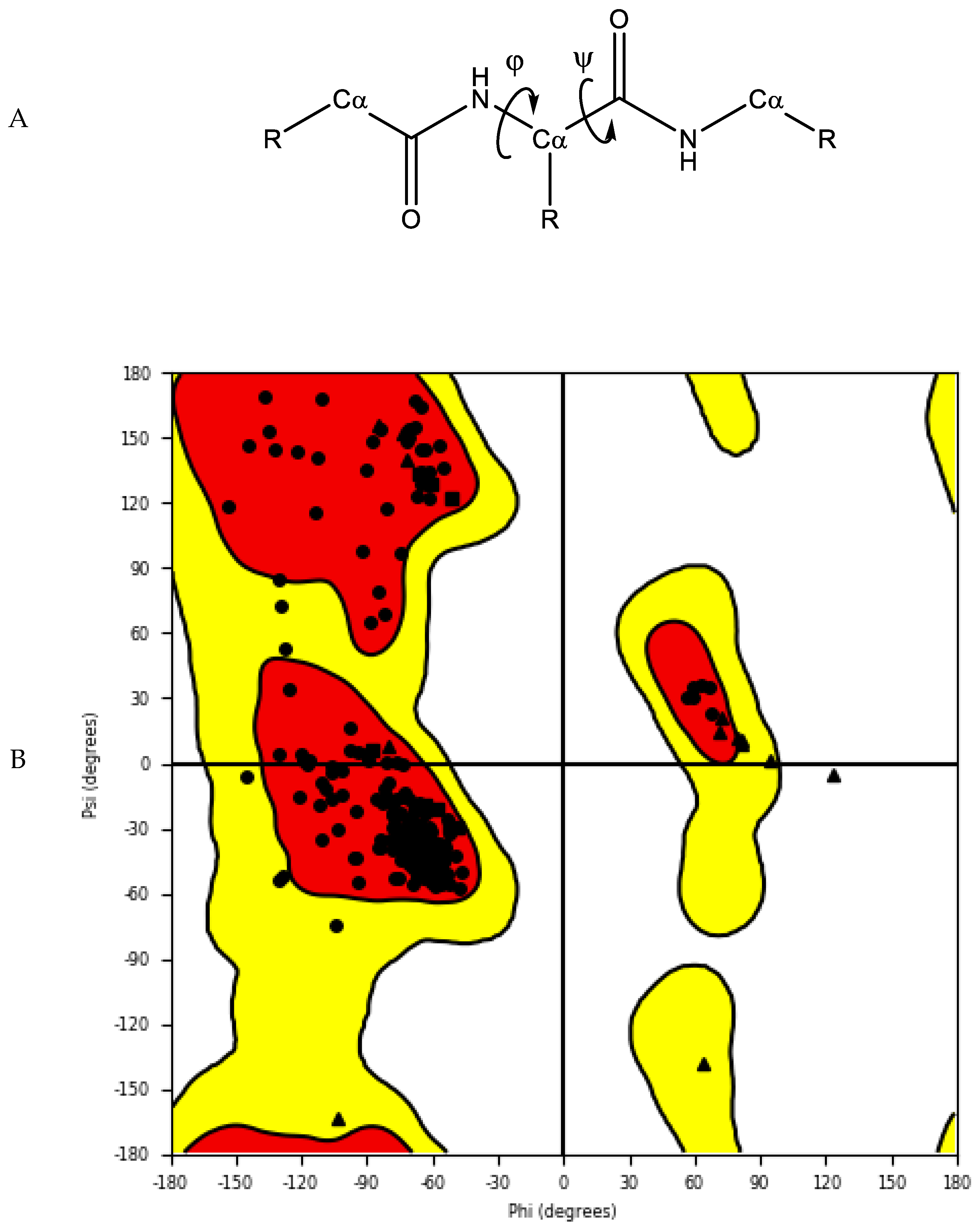
The accuracy and quality of the predicted structures can be validated and verified using different methods. The stereochemistry of the model can be verified by analysing bond lengths, torsion angles and rotational angles with tools, such as WHATCHECK [79] and Ramachandran plots [80]. The Ramachandran plot examines the backbone dihedral angles ϕ and ψ, which represents the rotations made by N—Cα and Cα—C bond in the polypeptide chain, respectively (Figure 5). Torsion angles determine the conformation of each residue and the peptide chain; however, some angle combinations cause close contacts between atoms, leading to steric clashes. The Ramachandran plot determines which torsional angles of the peptide backbone are permitted, and thus assesses the quality of the model. Spatial features, such as 3D conformation and mean force statistical potentials, can be validated using Verify3D [81], which measures the compatibility of the model to its own amino acid sequence. Each residue in the model is evaluated by its environment, which is defined by the area of the residue that is buried, the fraction of side-chain area that is covered by polar atoms (oxygen and nitrogen) and the local secondary structure. Other structure validation tools include MolProbity [82,83], NQ-Flipper [84], Iris [85], SWISS-MODEL [86] and Coot [87,88,89]. In addition to in silico validation, experimental validation of the predicted complexes may also be used to aid selection of a model for future in silico studies. Cross-linking mass spectrometry (XL-MS) provides experimental distance constraints, which can be checked against the predicted models [90].

2.2. Docking-Based Virtual Screening

Docking-based virtual screening aims to discover new drugs by predicting binding modes of both ligand and receptor, studying their interaction patterns, and estimating binding affinity. Some examples of the many docking programs include AutoDock [92], GOLD [93], Glide [94,95], SwissDock [96], DockThor [97], CB-Dock [98] and Molecular Operating Environment (MOE) [99] (Table 1). Due to limitations of X-ray crystallography and NMR spectroscopy, experimentally derived structures often have problems, such as missing hydrogen atoms, incomplete side-chains and loops, ambiguous protonation states and flipped residues. It is therefore essential to prepare the 3D structures accordingly in order to fix these issues before the docking process [100].

The three main goals of molecular docking are: (1) pose prediction to envisage how a ligand may bind to the receptor, (2) virtual screening to search for novel drug candidates from small molecule libraries and (3) binding affinity prediction using scoring functions to estimate the binding affinity of ligands to the receptor [101]. Search algorithms and scoring functions are essential components for molecular docking programs.

A good search algorithm should explore all possible binding modes, and this can be a challenging task. The concept of molecular docking originated from the ‘lock and key’ model proposed by Emil Fischer [102], and early docking programs treated both the protein and ligands as rigid bodies. It was known that protein and ligands are both dynamic entities and that their conformations play an important role in ligand–receptor binding and protein functions, but historically this was too computationally expensive to implement. Modern docking programs treat both protein and ligand with varying degrees of flexibility in order to address this issue.

2.2.1. Binding Site Detection

In docking-based virtual screening, the location of the binding site within the protein must be identified. Most of the protein structures in the PDB are ligand-bound (holo) structures, which defines the binding pocket and provides us with its geometries. In cases where only ligand-free (apo) structures available, there are traditionally three main types of method to identify potential druggable binding sites. Template-based methods such as firestar [103], 3DLigandSite [104] and Libra [105,106] utilise protein sequences to locate residues that are conserved and important for binding. Geometry-based methods, such as CurPocket [98], Surfnet [107] and SiteMap [108,109], search for clefts and pockets based on the size and depths of these cavities. Energy-based methods such as FTMap [110] and Q-SiteFinder [111] locate sites on the surface of a protein that are energetically favourable for binding. Hybrid methods, such as ConCavity [112] and MPLs-Pred [113], as well as machine-learning methods, such as DeepSite [114], Kalasanty [115], and DeepCSeqSite [116] are some of the newer approaches that are under rapid development in recent years.

Beyond locating the orthosteric binding site, these tools are also valuable in identifying potential allosteric binding sites to modulate protein function, hot spots on protein surface to alter protein–protein interactions and also analysing known binding sites to design better molecules that complement the binding pocket. Furthermore, proteins are dynamic systems, and their conformations may change upon ligand binding. Hidden binding pockets, known as cryptic pockets, which are not present in a ligand-free structure, can result from conformational changes upon ligand binding. Detection of cryptic pockets can be a solution to target proteins that were previously considered to be undruggable due to the lack of druggable pockets [117,118].

In addition to the location of the binding site, the evaluation of its potential druggability is equally important. Druggability is the likelihood of being able to modulate a target with a small molecule drug [119]. It can be evaluated on the basis of target information and association, such as protein sequence similarity or genomic information [120]. However, this approach only works for well-studied protein families and homologous proteins may not necessarily bind to structurally similar molecules [121].

Various efforts have been made to evaluate druggability using structure-based approaches. Cheng et al. developed the MAP_POD score, one of the first methods to evaluate druggability, using a physics-based method. MAP_POD model is a binding free energy model combined with curvature and hydrophobic surface area to estimate the maximal achievable affinity for passively absorbed drugs [119]. Halgren developed Dscore, which is a weighted sum of size, enclosure and hydrophobicity [108,109,122]. Other methods to predict druggability include Drug-like Density (DLID) [123], DrugPred [124], DoGSiteScorer [125], FTMap [126] and PockDrug [127].

DoGSiteScorer is a webserver that supports the prediction of potential pockets, characterisation and the druggability estimation. The algorithm first maps a rectangular grid onto the protein; grid points are labelled as either free or occupied depending on whether they lie within the vdW radius of any protein atom. Free grid points are merged to form pockets and subpockets, and neighbouring subpockets are then merged to form pockets. A 3D Difference of Gaussian (DoG) filter is then applied to identify pockets that are favourable to accommodate a ligand. These pockets are characterised global and local descriptors, such as pocket volume, surface, depth, ellipsoidal shape, types of amino acids, presence of metal ions, lipophilic surface, overall hydrophobicity ratio, distances between functional group atoms and many more [125,128].

To predict druggability, a machine learning technique (support vector machine model) trained on a set of known druggable proteins is used to identify druggable pockets based on a subset of these descriptors and to provide a druggability score between 0 to 1, where the higher the score the more druggable is the pocket. A SimpleScore, a linear regression based on size, enclosure and hydrophobicity, is also available to predict druggability [129].

Michel and co-workers used DoGSite, along with FTMap, CryptoSite, as well as SiteMap to predict ligand binding pockets and evaluate druggability of the nucleoside diphosphates attached to sequence-x (NUDIX) hydrolase protein family. Using a dual druggability assessment approach, the authors identified several proteins that are druggable out of the 22 that were studied. This in silico data was also found to correlate well with experimental results [130].

Sitemap locates binding sites by placing ‘site points’ around the protein and each site point is analysed for the proximity to the protein surface and solvent exposure. Site points that fulfil the criteria and are within a given distance of each other are combined into subsites, then subsites that have a relatively small gap between them in a solvent-exposed region are merged to form sites. Distance-field and van der Waals (vdW) grids are then generated to characterise the binding site into three basic regions: hydrophobic, hydrophilic (further separates into H-bond donor, acceptor, and metal-binding region) and neither. Sitemap also evaluates the potential binding sites and computes various properties such as size of the site measured by number of site points, exposure to solvent, degree of enclosure by protein, contact of site points with the protein, hydrophobic and hydrophilic character of the site, and the degree to which a ligand can donate hydrogen bonds. These properties contribute to the calculation of the SiteScore (to distinguish drug-binding and non-drug binding sites) and Dscore (druggability score), which helps to recognise druggable binding sites for virtual screening [108,109].

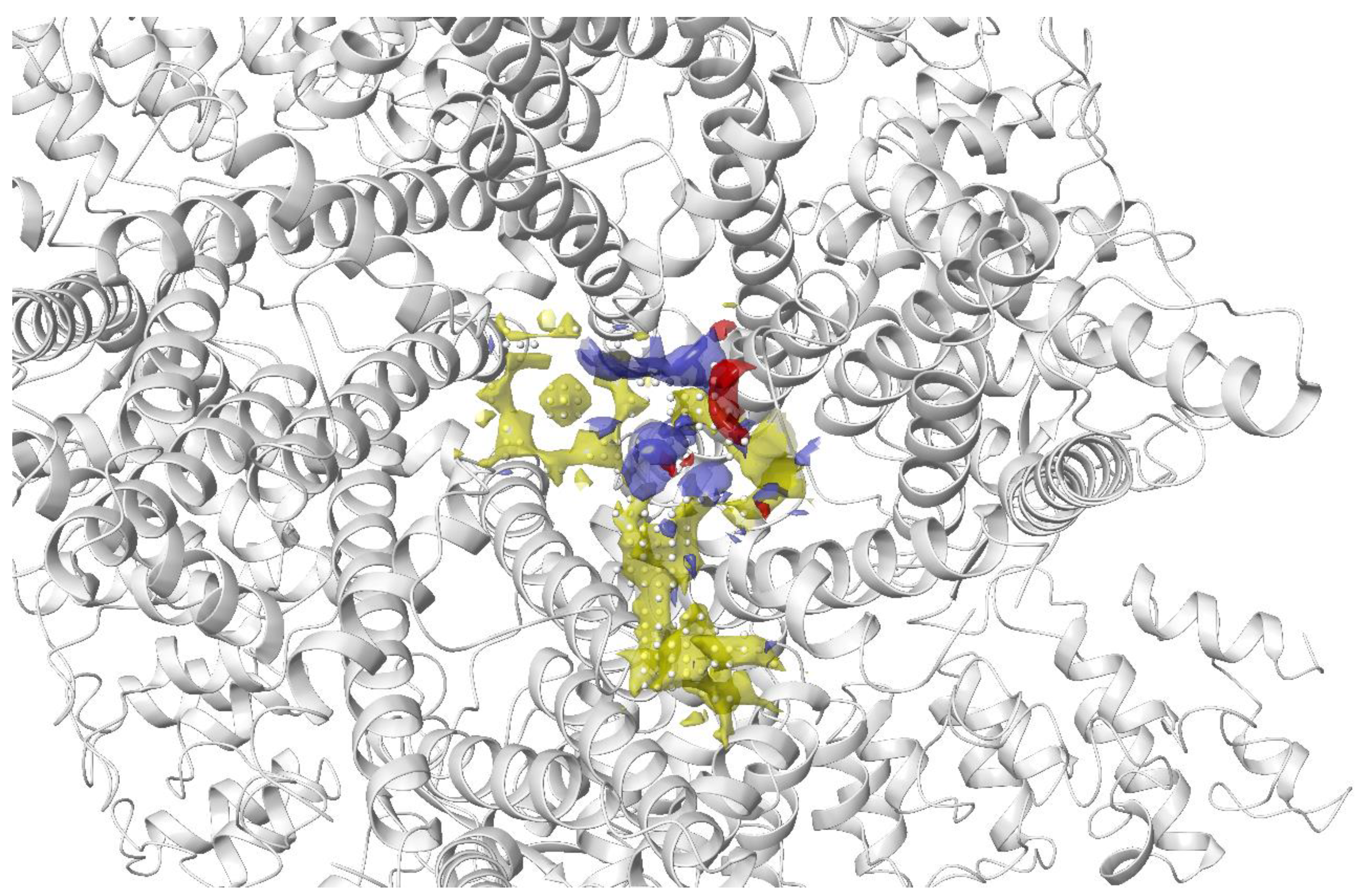
The transient receptor potential vanilloid 4 (TRPV4) is a widely expressed non-selective cation channel involved in various pathological conditions. Despite the availability of several TRPV4 inhibitors, the binding pocket of TRPV4 and the mechanism of action was not well understood. Doñate-Macian and coworkers used Sitemap to search and assess the binding pocket for one of the known TRPV inhibitors HC067047 based on the crystal structure of Xenopus TRPV4 (Figure 6). This group also further characterised the binding pocket and inhibitor–protein binding interactions with the aid of molecular docking, molecular dynamics and mutagenesis studies. The information was then employed to run a structure-based virtual screening to discover novel TRPV4 inhibitors [131].

2.2.2. Ligand Flexibility

Ligand structures for virtual screening can be obtained from small molecule databases, which are free (e.g., ZINC [132], DrugBank [133] and Pubchem [134]) or commercial (e.g., Maybridge, ChemBridge and Enamine). Conformational sampling of ligands can be performed in several ways. Systematic search generates all possible ligand conformations by exploring all degrees of freedom of the ligand [135]. Carrying out a systematic search using a brute-force approach (exhaustive search) can easily overwhelm the computing power, especially for molecules with many rotatable bonds and therefore rule-based methods have been the more favoured approaches in recent years. Rule-based methods, such as the incremental construction algorithm (also known as anchor and grow method), generate conformations based on known structural preferences of compounds by limiting the conformational space that is being explored. Usually, a knowledge base of allowed torsion angles and ring conformations (e.g., data from the PDB), and possibly a library of 3D fragment conformations, is used to guide the sampling [136,137]. These break the molecule into fragments that are docked into different regions of the receptor. The fragments are then reassembled together to construct a molecule in a low energy conformation.

Conformer generator OMEGA [138] employs a prebuilt library of fragments as well as a knowledge base of torsion angles to generate a large set of conformations, which are sampled by geometric and energy criteria to eliminate conformers with internal clashes. Likewise, ConfGen [139] divides ligands into a core region and peripheral rotamer groups. The core conformation is first generated using a template library, followed by the calculation of the potential energy of rotatable bonds with the torsional term of the OPLS force field, and lastly positioning peripheral groups in their lowest energy forms. To eliminate undesirable conformations or to limit the number of conformations, filtering approaches are applied. Conformations that are too similar are removed based on an energy filter, RMSD, and dihedral angles involving polar hydrogen atoms. Compact conformers are also removed by an empirically derived heuristic scoring method [94,139].

On the other hand, a stochastic search randomly changes the degrees of freedom of the ligand at each step and the change is either accepted or rejected according to a probabilistic criterion such as the Metropolis criterion [140]. Sampling of conformational space can be performed using different techniques in a stochastic search, including Monte Carlo (MC) sampling [62], distance geometry sampling [141] and genetic algorithm-based sampling [142,143]. Balloon [142], a free conformer generator, uses distance geometry to generate an initial conformer for a ligand, followed by a multi-objective genetic algorithm approach to modify torsion angles around rotatable bonds, stereochemistry of double bonds, chiral centres, and ring conformations. Some other tools that were developed for ligand preparation include Prepflow [144], VSPrep [145], Gypsum-DL [146], Frog2 [147] and UNICON [148].

2.2.3. Protein Flexibility

Protein flexibility is essential for their biological function and subtle changes, such as side-chain rearrangements, can alter the size and shape of the binding site and thus bias docking results [149]. Methods to handle protein flexibility can be divided into four groups: soft docking [150,151], side-chain flexibility [152], molecular relaxation [153], and protein ensemble docking [154,155]. Soft docking allows small degrees of overlap between the protein and the ligand by softening the interatomic vdW interactions in docking calculations [151]. These are the simplest methods and are computationally efficient, but they can only account for small changes. Side-chain flexibility allows the sampling of side-chain conformations by varying their essential torsional degrees of freedom, while the protein backbones are kept fixed [156]. The molecular relaxation method involves both protein backbone flexibility and side-chain conformational changes; it first uses rigid-protein docking to place the ligand into the binding site then relaxes the protein backbone and the nearby side-chain atoms, usually employing methods, such as MC and MD [157,158,159]. Protein ensemble docking methods dock the ligand on a set of rigid protein structures, with different conformations which represent a flexible receptor. The docking results for each conformation are then re-analysed [160].

Most contemporary docking approaches treat proteins with partial or complete flexibility. For instance, Schrödinger offers a range of docking methodologies with different treatment of protein flexibility. Glide [94,95], with standard precision (SP) and extra precision (XP) is a docking strategy, which allows conformational flexibility for the ligands but treats the receptor as a rigid entity. It softens the active site via vdW scaling (soft docking) with the option of rotamer configuration sampling. Meanwhile, a superior method, Induced Fit Docking, uses Glide for docking to account for ligand flexibility, and Prime [161,162] for side-chain optimisation to account for receptor flexibility [163]. The ligand is docked into the receptor using Glide with vdW scaling and flexible side-chains are temporarily mutated to alanine to reduce steric clashes and the blocking of the binding site. Once the docking poses are generated, the mutated residues are restored to their original residues and Prime (a program for protein structure predictions) [161,162] is used to predict and reorient the side-chains with each ligand pose. The ligand–receptor complex is then minimised to afford a low-energy protein conformation, which is used for ligand resampling with Glide.

Water molecules have a crucial role in biological systems and interactions, such as stabilising protein–ligand complex, biomolecular recognition and participating in H-bond networks. Water molecules can participate in ligand–protein interactions by acting as bridging waters, and their displacement from the binding site upon ligand binding can also contribute to binding affinity, playing a significant role in the thermodynamics of protein-ligand binding [164]. The retention or removal of water molecules during virtual screening can have a direct impact on the size, shape and chemical properties of the binding site, which can influence binding geometries and affinity calculations.

Due to the ability of a water molecule to act as both an H-bond donor and acceptor, as well as its highly mobile nature, predicting the location and contribution of water molecules in protein–ligand binding is a challenging task. Crystal structures or cryo-EM structures of proteins can sometimes capture the placement of water molecules in the protein matrix, but the information is not always accurate due to the low resolution of the structural data, and the sample preparation conditions do not reflect the biological environment [165,166,167,168].

Many approaches were developed to simulate and predict the behaviour of water molecules. Implicit models, also known as continuum models, treat water molecules as a uniform and continuous medium. The free energy of solvation is traditionally estimated based on three parameters, the free energy required to form the solute cavity, vdW interactions and electrostatic interactions between solute and solvent. This method is less computationally demanding but neglects details at the solute–solvent interface [167,168]. Explicit models are computationally more expensive, but the molecular details of each water molecule are considered. Water molecules are normally described using a three-, four-, or five-point model.

In protein–ligand docking, water can be treated explicitly or in an approach involving a combination of implicit and explicit (hybrid), and they can be separated into four categories: (1) Empirical and knowledge-based methods (e.g., Consolv [169] and WaterScore [170]), (2) statistical and molecular mechanics methods (e.g., GRID [171,172], 3D-RISM [173,174], SZMAP [175]), (3) MD simulation methods (e.g., WaterMap [176], GIST [177], SPAM [116]) and, lastly, (4) Monte Carlo simulation methods (e.g., JAWS [178]).

2.2.4. Scoring Functions

After searching for all possible binding modes, a scoring function is used to evaluate the quality of the docking poses. Scoring functions determine the binding mode and estimate binding affinity, which assists in identifying and ranking potential drug candidates. There are three main categories of scoring functions: force field-based, empirical-based, and knowledge-based methods.

Force field-based scoring functions generally use standard force field parameters taken from force fields, such as AMBER [179], which consider both the intramolecular energy of the ligand and the intermolecular energy of the protein–ligand complex [180]. The ΔG estimated using this scoring function is the sum of these energies, which is generally composed of vdW and electrostatic energy terms. An example of program that uses this method is DOCK, which utilises the following equation: [181,182]

$$\Delta G={\displaystyle \sum }_i{\displaystyle \sum }_j\left(\frac{A_{ij}}{r_{ij}^{12}} - \frac{B_{ij}}{r_{ij}^6}+\frac{q_i{q}_j}{\epsilon \left(r_{ij}\right)r_{ij}}\right)$$

(1)

where ${\mathrm{r}}_{ij}$ is the distance between protein atom $i$ and ligand atom $j$, $A_{ij}$ and $B_{ij}$ are vdW components (repulsive and attractive vdW), $q_i$ and q_j are atomic charges and $\epsilon \left(r_{ij}\right)$ is the distance-dependent dielectric constant.

Empirical-based functions estimate binding affinity based upon a set of weighted energy terms that are described in the following equation:

$$\Delta G={\displaystyle \sum }_i{W}_i · \Delta G_i$$

(2)

The energy terms ($\Delta G_i$) represents energy terms such as vdW energy, electrostatic energy, hydrogen (H) bond interactions, desolvation, entropy, hydrophobicity, etc., whereas the weighting factors ($W_i$) are determined via regression analysis by fitting the binding affinity data of a training set of protein–ligand complex with known 3D structures [94]. The first empirical scoring function (SCORE) was developed by Böhm in 1994 [183] based upon a dataset of 45 protein–ligand complexes, and the scoring function considers four energy terms: hydrogen bonds, ionic interactions, the lipophilic protein–ligand contact surface and the number of rotatable bonds in the ligand. Over time, the empirical scoring function has evolved by expanding the data set and considering more energy terms. For example, ChemScore, developed by Eldridge et al. [184], also considers metal atoms contribution and Glide XP score includes terms to account for desolvation effects [94].

In knowledge-based functions, structural information is extracted from experimentally determined structures of protein–ligand complexes from databases, such as the PDB [30] and Cambridge Structural Database (CSD) [185,186]. Boltzmann law is employed to transform the protein–ligand atom pair preferences into distance-dependent pairwise potentials, and the favourability of the binding modes of atom pairs is related to the frequency observed in known protein–ligand structures [187,188]. The potentials are calculated using the following equation:

$$\mathrm{w}\left(\mathrm{r}\right)=-{ K}_{\mathrm{B}}T\ln \left[\mathrm{g}\left(\mathrm{r}\right)\right], \mathrm{g}\left(\mathrm{r}\right)=\rho \left(\mathrm{r}\right)/\rho \ast \left(\mathrm{r}\right)$$

(3)

where w(r) is the pairwise potential between protein and ligand, $K_{\mathrm{B}}$ is the Boltzmann constant, $T$ is the absolute temperature of the system, $\rho \left(\mathrm{r}\right)$ is the number density of the protein–ligand atom pair at distance $\mathrm{r}$, and $\rho \ast \left(\mathrm{r}\right)$ is the pair density in a reference state where the interatomic interactions are zero.

Table 1. List of common docking programs.

Program	Ligand Flexibility	Receptor Flexibility	Scoring Functions	Examples of Application
Glide (HTVS, SP and XP) [94,95,189]	Exhaustive ligand conformation search	Soft docking	Empirical	Discovery of novel fibroblast growth factor receptor 1 kinase inhibitors [190] and CDK5 inhibitors [191]
GOLD [93]	Genetic algorithm	Soft docking Ensemble docking Side-chain flexibility	Goldscore (empirical) Chemscore (empirical) ChemPLP (empirical) ASP (knowledge based)	Design of non-peptide MDM2 inhibitors [192]
Autodock 4 [193]	Genetic Algorithm Simulated Annealing Local Search Lamarckian Genetic Algorithm	Side-chain flexibility	Semi-empirical free energy force field	Discovery of reversible NEDD8 activating enzyme inhibitor [194]
DOCK 6 [195]	Incremental construction algorithm	Rigid	Force field	Design and development of potent and selective dual BRD4/PLK1 Inhibitors [196]
Internal Coordinates Mechanics (ICM) [197]	Stochastic search (MC)	Side-chain flexibility (rotamer libraries)	Force field	Discovery of novel retinoic acid receptor agonist [198] and enoyl-acyl carrier protein reductase inhibitors in Plasmodium falciparum [199]
Surflex [200,201]	Incremental construction algorithm	Ensemble docking	Empirical	Discovery of novel inhibitors of Leishmania donovani γ-glutamylcysteine synthetase [202]
MOE [99,203,204,205]	Systematic (exhaustive) Stochastic High throughput Conformational Import (incremental construction + stochastic) [99]	Rigid	ASE (empirical) Affinity dG (empirical) Alpha HB (empirical) GBVI/WSA (force field)	Identification of novel monoamine oxidase B inhibitors [206] and Chk1 inhibitors [207]
FlexX [208,209]	Incremental construction algorithm	Rigid	Empirical	Identification of PKB inhibitors [210] and phosphodiesterase 4 inhibitors [211]
FRED [212,213]	Systematic (exhaustive) search, precomputed using Omega (using torsion and ring libraries) [138]	Rigid	Chemgauss 3 (empirical) Chemgauss 4 (empirical)	Discovery of selective butyrylcholinesterase inhibitors [214]

Abbreviations: ASP: Astex Statistical Potential; BRD4: Bromodomain 4; CDK5: Cyclin dependent kinase 5; ChemPLP: Piecewise Linear Potential; HTVS: high throughput virtual screening; MDM2: Mouse double minute 2 homolog; PKB: Protein kinase B; PLK1: Polo-like Kinase 1.

Table 1. List of common docking programs.

Program	Ligand Flexibility	Receptor Flexibility	Scoring Functions	Examples of Application
Glide (HTVS, SP and XP) [94,95,189]	Exhaustive ligand conformation search	Soft docking	Empirical	Discovery of novel fibroblast growth factor receptor 1 kinase inhibitors [190] and CDK5 inhibitors [191]
GOLD [93]	Genetic algorithm	Soft docking Ensemble docking Side-chain flexibility	Goldscore (empirical) Chemscore (empirical) ChemPLP (empirical) ASP (knowledge based)	Design of non-peptide MDM2 inhibitors [192]
Autodock 4 [193]	Genetic Algorithm Simulated Annealing Local Search Lamarckian Genetic Algorithm	Side-chain flexibility	Semi-empirical free energy force field	Discovery of reversible NEDD8 activating enzyme inhibitor [194]
DOCK 6 [195]	Incremental construction algorithm	Rigid	Force field	Design and development of potent and selective dual BRD4/PLK1 Inhibitors [196]
Internal Coordinates Mechanics (ICM) [197]	Stochastic search (MC)	Side-chain flexibility (rotamer libraries)	Force field	Discovery of novel retinoic acid receptor agonist [198] and enoyl-acyl carrier protein reductase inhibitors in Plasmodium falciparum [199]
Surflex [200,201]	Incremental construction algorithm	Ensemble docking	Empirical	Discovery of novel inhibitors of Leishmania donovani γ-glutamylcysteine synthetase [202]
MOE [99,203,204,205]	Systematic (exhaustive) Stochastic High throughput Conformational Import (incremental construction + stochastic) [99]	Rigid	ASE (empirical) Affinity dG (empirical) Alpha HB (empirical) GBVI/WSA (force field)	Identification of novel monoamine oxidase B inhibitors [206] and Chk1 inhibitors [207]
FlexX [208,209]	Incremental construction algorithm	Rigid	Empirical	Identification of PKB inhibitors [210] and phosphodiesterase 4 inhibitors [211]
FRED [212,213]	Systematic (exhaustive) search, precomputed using Omega (using torsion and ring libraries) [138]	Rigid	Chemgauss 3 (empirical) Chemgauss 4 (empirical)	Discovery of selective butyrylcholinesterase inhibitors [214]

Abbreviations: ASP: Astex Statistical Potential; BRD4: Bromodomain 4; CDK5: Cyclin dependent kinase 5; ChemPLP: Piecewise Linear Potential; HTVS: high throughput virtual screening; MDM2: Mouse double minute 2 homolog; PKB: Protein kinase B; PLK1: Polo-like Kinase 1.

3. Ligand-Based Drug Design

When there is limited structural knowledge on the target protein, biological and chemical information is drawn from known active ligands to identify key features that are responsible for biological activity and this information can be used for ligand-based drug design (LBDD). Common LBDD methods include similarity searches, scaffold hopping, quantitative structure–activity relationship (QSAR) and pharmacophore models. Although CADD approaches are generally classified as structure-based and ligand-based approaches, it should be noted that virtual screening strategies often integrate and combine the two to improve the success rate in hit identification [215].

3.1. Similarity Search

The underlying hypothesis of molecular similarity is that molecules with similar molecular structures have similar physical properties and biological activities. Two key components in similarity analysis are structural representations and quantitative measurements of similarity between the two structural representations.

Different molecular fingerprints can be used to represent the chemical properties of a molecule, and similarity measurements can rely on the use of 1D, 2D and 3D descriptors. This involves dividing the molecule into a sequence of bits; so, the common bits between molecules can be compared to assess similarity. Some common molecular fingerprints include structural keys, topological fingerprints, circular fingerprints and pharmacophore fingerprints [216]. Structural key fingerprints, such as the MACCS fingerprint [217] and TGD fingerprint [218], search for the presence of structures/features of the molecules based on a pre-defined list of structural keys. This method is most useful when the molecules contain a lot of structural keys. Topological fingerprints (e.g., Daylight fingerprint) [219] analyse the fragments of the molecule following a connectivity path (usually linear) up to a certain number. The algorithm generates a pattern for each atom in the molecule, then a pattern for each atom and its nearest neighbours and connecting bonds, followed by a pattern that represents each group of atoms and bonds connected by paths up to two bonds long, and the process continues with longer bond paths. Circular fingerprints, such as Molprint2D [220] and extended-connectivity fingerprints (ECFP) [221], look at the environment of each atom in the molecules up to a certain radius. Every heavy atom of a molecule is sequentially used as a starting point and is assigned an atom type. This is followed by the assignment of atom types to neighbouring atoms of the central heavy atoms (first layer). This process is repeated with each distance/layer from the central heavy atom and the number of atoms with each given atom type are recorded to calculate descriptor values [222]. In addition to the common molecular fingerprints mentioned that are mostly used to describe synthetic compounds, the Natural Compound Molecular Fingerprint (NC-MFP) was developed by Seo et al. to better represent natural products [223].

There are different metrics that can be used to assess and quantify the similarity between two molecules (A and B). Most metrics have the range from 0 (completely dissimilar) to 1 (identical). Some of the common metrics are listed below:

Tanimoto coefficient (range: 0–1): [224]

$$S=\frac{c}{a+b-c}$$

(4)

Dice index (range: 0–1): [225]

$$S=\frac{2c}{\left(a+b\right)}$$

(5)

Cosine coefficient (range: 0–1): [226]

$$S=\frac{c}{\sqrt{ab}}$$

(6)

Euclidean distance (range: 0–1): [226]

$$D=\sqrt{a+b-2c}$$

(7)

where $a$ is the number of bits present in molecule A, $b$ is the number of bits present in molecule B and $c$ is the number of bits present in both molecule A and B. $S$ denotes similarities and $D$ denotes distances where $S=\frac{1}{1+D}$. The cut-off values for the similarity metrics depend on both the fingerprints and metrics used and hence cannot be compared directly. For example, WebCSD, the online portal to CSD, offers both the Tanimoto coefficient and the Dice index for similarity search and the default cut-off values were set as 0.7 and 0.975, respectively [227].

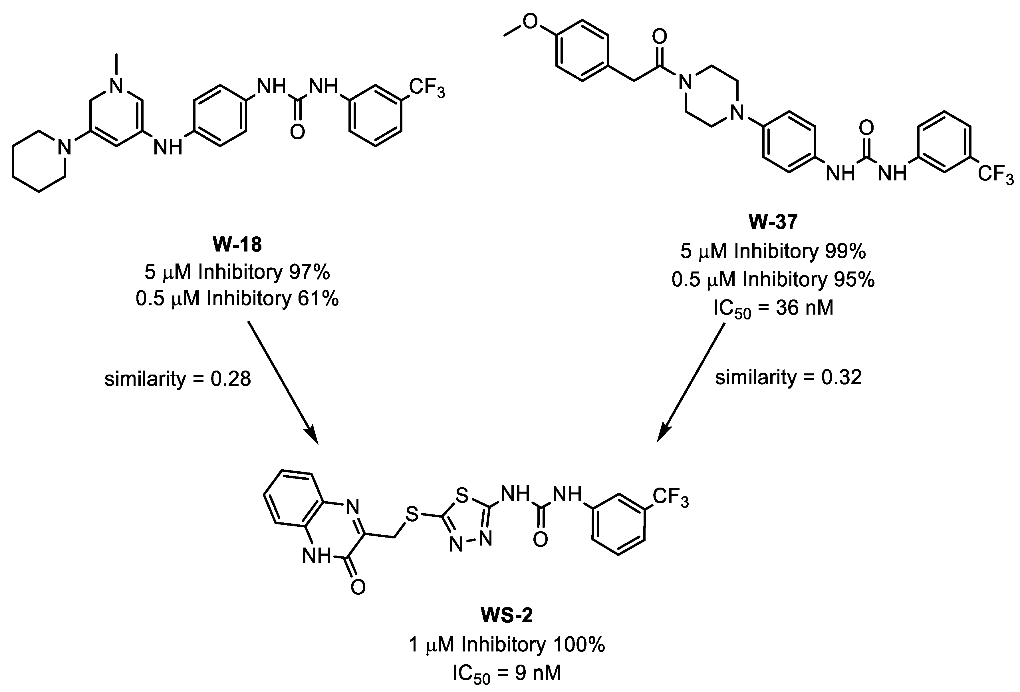
Wang and co-workers used a combination of docking-based and 2D similarity search techniques to identify novel CDK8 inhibitors [228]. A small molecule library was first subjected to molecular docking against multiple crystal structures of CDK8 to account for the protein conformation change. Of the 50 candidates selected from the docking study, 7 showed more than 30% inhibition against CDK8 based on in vitro binding competition assay. Similarity search using Discovery Studio [229] was performed on W-18 and W-37, two of the most potent candidates, to find similar structures with high CDK8 inhibitory effects. Using the Tanimoto coefficient to calculate the similarities of molecules based on the ECFP_6 fingerprints, WS-2 which shares 0.28 and 0.32 similarity with W-18 and W-37, respectively, was identified and it is significantly more potent than both of the parent molecules (Figure 7).

3.2. Quantitative Structure-Activity Relationship (QSAR)

A QSAR model is a computational or mathematical model that derives correlation between the calculated molecular properties of a group of compounds and their experimentally determined activity. QSAR methodology was first proposed by Hansch and Fujita in 1964 who published a method for the correlation of biological activity and chemical structure [230], and QSAR methodology has evolved a lot since then. 1D- and 2D-QSAR models are classified as ‘classical’ QSAR methodologies, where 1D-QSAR correlates biological activity with molecular properties, such as pKa and logP [231], and 2D-QSAR correlates biological activity with the structure of the ligands on a 2D basis and considers descriptors, such as topological and constitutional descriptors [230,232]. Topological descriptors are based on the connectivity of atoms in the molecule, including molecular size, shape, branching, heteroatoms and multiple bonds but with no information on the 3D spatial arrangement of the atoms [181]. Constitutional descriptors simply describe the molecular composition of a molecule, such as molecular weight, number of atoms and bonds, types of atoms, and ring counts.

3D-QSAR takes into account the 3D spatial representation of molecules, such as different conformations and stereo-isomerisation. Two of the most popular 3D-QSAR methodologies are the Comparative Molecular Field Analysis (CoMFA) proposed by Cramer et al. [233] and the Comparative Molecular Similarity Indices Analysis (CoMSIA) proposed by Klebe et al., a modified version of CoMFA [234]. The primary goal of 3D-QSAR is to establish a relationship between biological activity and spatial properties of the ligands, therefore data quality and structural diversity are particularly important to construct a good quality 3D-QSAR model. 3D-QSAR is often used for lead optimisation and biological activity prediction for novel compounds as it can quantitatively correlate modifications in 3D chemical structures and the respective changes in biological effects.

For example, the 3D-QSAR method was applied in the structure–activity relationship (SAR) analysis of maslinic acid analogues and the identification of its anti-cancer target. Maslinic acid analogues are known to be anti-cancer compounds but there was no structural information about its molecular target. A common pharmacophore model on five analogues was first constructed, then field points-based descriptors were used to build a 3D-QSAR model after aligning 74 analogues to the pharmacophore model. A field point-based similarity search on maslinic acid was performed on the ZINC database, followed by screening through the 3D-QSAR model for bioactivity prediction and SAR field point’s compliance. Additional filters (Lipinski’s rule of five, absorption, distribution, metabolism, and excretion (ADME) and synthetic accessibility) were also applied and eventually 39 compounds were listed. The compounds were docked against a series of potential cellular targets of maslinic aid analogues (predicted by STITCH) [235] and identified NR3C1 as a major anti-cancer target of maslinic acid analogue as well as compound P-902 as a potential lead compound [236].

3.3. Pharmacophores

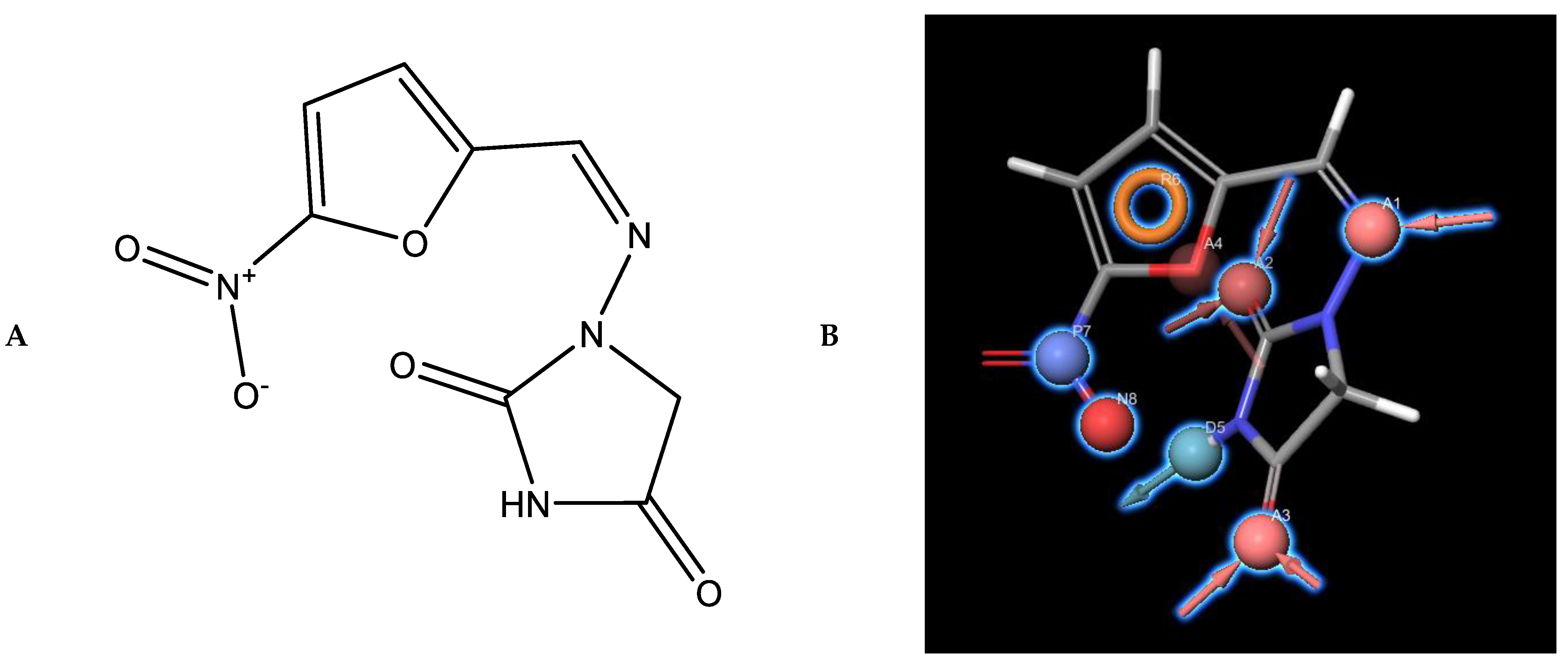
It is widely believed that Paul Ehrlich came up with the concept of pharmacophore: a molecular framework that carries (phoros) the essential features responsible for a drug’s (pharmacon) biological activity in the early 1900s [237,238]. However, some consider the concept of modern pharmacophore was in fact proposed by Schueler in 1960 [239], which was then extended by Beckett and co-workers who introduced the first pharmacophore model with identified distance ranges in 1963 [240] and Kier who proposed the first computed pharmacophore model in 1967 [241]. Nowadays, pharmacophore models are extractions of electronic and steric features from ligands in a 3D spatial arrangement that is relevant for interactions to the target protein and the relative biological responses. The features are purely abstract concepts and do not represent chemical functional groups or a typical structural skeleton [242]. The six classical pharmacophore features classified are H-bond donors, H-bond acceptors, negative ionic, positive ionic, hydrophobic regions, and aromatic regions (Figure 8). On top of that, less common features can also better characterise the chemical functionalities, such various metal binding locations are supported by LigandScout [243,244,245,246]. Constraints and restrictions can also be applied by introducing excluded volumes to the model to prevent ligands from occupying certain spaces (ligand-inaccessible) [247]. Pharmacophores can be divided into two sub-categories: ligand-based and structure-based pharmacophores.

Ligand-based pharmacophores are based on the chemical structures of ligands when there is little structural information about the target protein is available. To construct a ligand-based pharmacophore, the conformational space of flexible active molecules (through conformational sampling) is covered because the molecules should be in their bioactive conformations. The molecules are then aligned, and common features are extracted to generate a pharmacophore model. Alignment techniques are divided into point-based and property-based approaches [248]. In point-based approach, atoms, fragments, or chemical feature point distances are minimised, and pairs of points are superimposed by minimising distances. Some examples of programs that use point-based alignment include HipHop [249], Phase [250,251] and Galahad [252]. In contrast, property-based approaches (e.g., MOE [99]) generate alignments based on molecular field descriptors, such as electron density, electrostatic potential, molecular shape and volume, etc. [248,253].

A study conducted by Rampogu et al. developed a ligand-based pharmacophore model for the screening of natural compounds against HER2 kinase domain. A total of 82 compounds with various levels of activity were chosen from the literature where 32 of them were used to construct a pharmacophore model using Discovery Studio [229]. The rest of the compounds, together with decoy set, were employed to validate the model. A total of 197 201 compounds from the Universal Natural Products Database were first filtered for ADME and Lipinski’s Rule of Five to identify compounds with drug-like properties, followed by screening against the pharmacophore model. The resulting compounds were subjected to molecular docking and MD simulations and eventually identified two potential leads against HER2 breast cancers [254].

One of the biggest drawbacks in ligand-based pharmacophore modelling is the selection of training set ligands. Searching for active ligands to form a training set from the literature could be a difficult task as biological assays were conducted under different experimental conditions. Performing biological assays, such as enzyme kinetic assays, under consistent conditions can be useful to investigate relative biological activities of the ligands, and hence the direct ligand–protein interactions. Although highly different pharmacophore models can increase diversity and cover wider chemical space, training set ligands with larger structural differences might require other experimental validation (e.g., X-ray crystal structure) to confirm they share the same binding site. Nevertheless, the real problem of ligand-based pharmacophore modelling lies in defining if a ligand is active or inactive, particularly in the case of defining qualitative pharmacophores. The diversity of the dataset could hugely affect the pharmacophore model generated, including feature types, locations and excluded volumes [255].

Compared to ligand-based pharmacophores, structure-based approaches are less likely to be biased by the chemical structures of existing active compounds and thus yield more diverse molecules. Structure-based pharmacophore models are constructed from either a protein–ligand complex or from the 3D structure of the receptor alone (receptor-based). The protein–ligand complex approach evaluates the key interactions between the ligand and the binding site and then transforms this information into a pharmacophore model [256]. For cases where the structural information of the ligand is lacking, the receptor-based approach can be applied. Pharmacophore hypotheses can be derived from protein structures using two methods: geometric constraints [257] and binding site analysis using virtual probe atoms [258].

MurG is one of the enzymes involved in the biosynthesis of the peptidoglycan layer in Mycobacterium tuberculosis and inhibition of MurG could be useful for the treatment of tuberculosis. Saxena et al. built a pharmacophore model based on the protein–ligand interactions of the homology model of Mycobacterium tuberculosis MurG due to the lack of available crystal structures. The pharmacophore model, along with molecular docking and MD simulations, was used and identified three lead compounds that were potential Mycobacterium tuberculosis MurG inhibitors [259].

3.3.1. Pharmacophore Validation

Before employing the pharmacophore model for virtual screening, it is essential to validate the model to evaluate the predictivity of the model. Decoys databases such as DUD-E [260], MUV [261] and DEKOIS [262] are often used to test the model’s ability to differentiate active and inactive compounds. Multiple refinements are frequently performed to result a better model after testing with different metrics. Examples of some of the commonly used metrics are listed below:

Yield of actives ($Ya$) shows the retrieved true positive compounds ($Ha$) in relation to the number of hits retrieved ($Ht$) [263].

$$Ya=\frac{Ha}{Ht}$$

(8)

Sensitivity ($Se$) is the ratio Ha to all the actives compounds ($A$) in the database. The closer the number is to 1, the higher number of active compounds returned from the search. It gives an insight into the ability of the model to select truly active compounds [264].

$$Se=\frac{Ha}{A}$$

(9)

Specificity ($Sp$) is the ratio of rejected true negatives ($TN$) to all the–inactive compounds ($D-A$), where $D$ is the number of entries in the database). When $Sp$ = 1, all the inactive compounds have been correctly rejected. Specificity tells us the ability of the model to discard inactive compounds [264].

$$Sp=1-\frac{Ht-Ha}{D-A}$$

(10)

Enrichment factor ($EF$) measures $Ya$ proportional to the ratio of $A$ in the whole database [264].

$$EF=\frac{Ya}{A/D}=\frac{Ha/Ht}{A/D}$$

(11)

The Goodness of Hit list ($GH score$) is a combination of sensitivity, specificity, and yield of actives of different weightings. It considers both true actives ratio and true inactives ratio, which makes it a very powerful tool [265]. The GH score ranges from 0 (null model) to 1 (ideal model), a model with a GH score > 0.6 is generally expected to be reliable [266].

$$GH score=\left(\frac{3}{4}·Ya+\frac{1}{4}·Se\right)·Sp=\left(\frac{Ha\left(3A+Ht\right)}{4HtA}\right)\left(1-\frac{Ht-Ha}{D-A}\right)$$

(12)

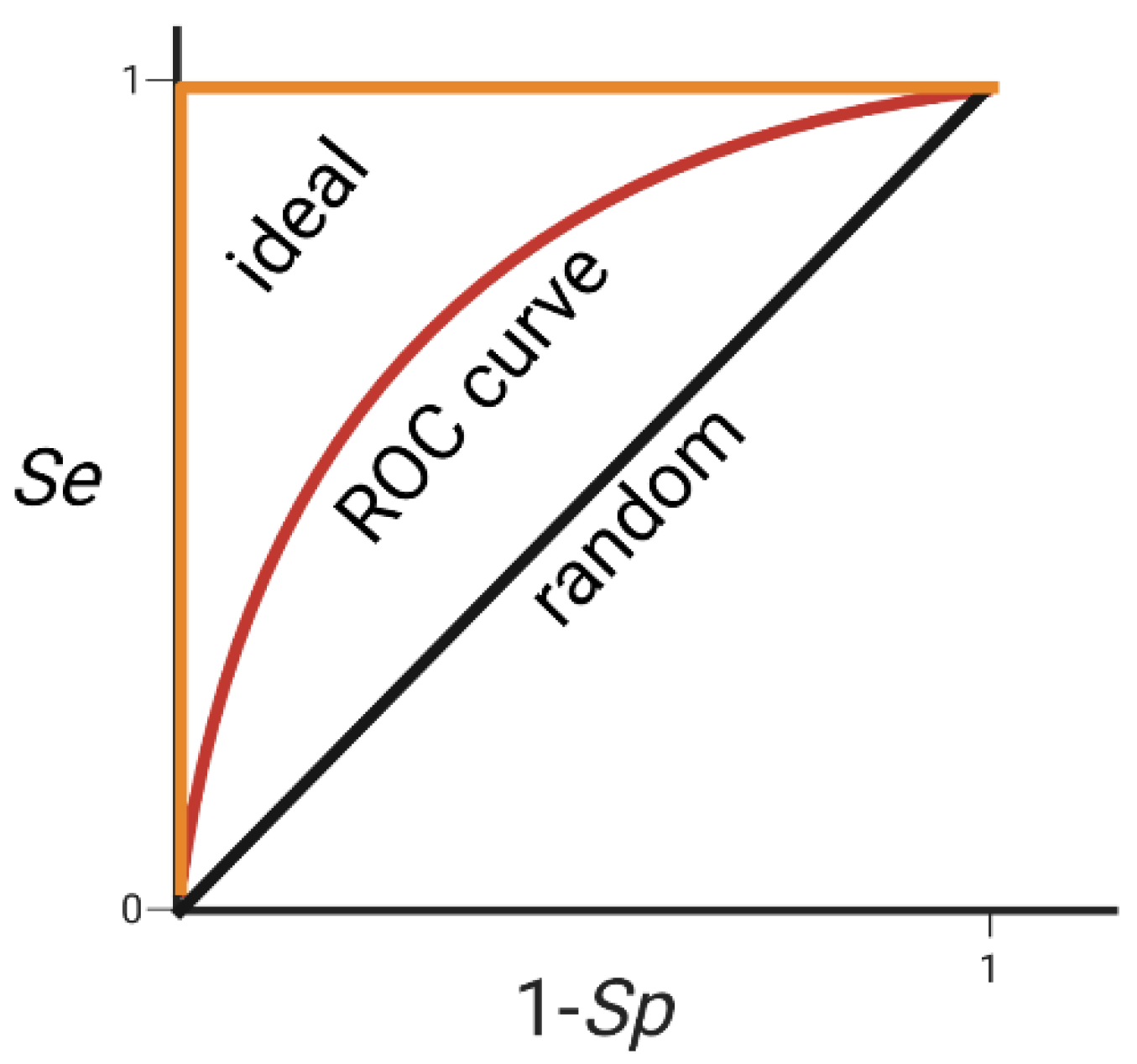
The Receiver operative characteristic (ROC) curve displays the increase of false positives that results with increased true positives. On the Y-axis the true-positive rate ($Se$) is represented, and on the X-axis the false-positive rate (1 − $Sp$) is represented. The area under the curve (AUC) is normally used to measure the performance of the model. The greater the AUC (ideal value is 1), the better is the model. An AUC of 0.5 indicates a random database search and thus a poor model (Figure 9) [267].

3.3.2. Pharmacophore Screening

Once the model is validated, databases of small molecules are screened against the pharmacophore model (query) and molecules that match with the features in the model will be extracted and identified as hit compounds. Other than ligand alignment, conformational flexibility is the other big challenge that is encountered in pharmacophore-based virtual screening. In general, conformations of ligands can either be pre-enumerated before the screening process, or conformation search is performed on-the-fly in the pharmacophore fitting process [268]. Pre-enumeration is less computationally expensive but requires bigger storage space, whereas conformation search on-the-fly is time consuming and requires more computer power. Some common pharmacophore screening programs include Catalyst [249], Phase [250,251], LigandScout [269], PharmID [270].

Recently, Dong and co-workers discovered an anti-fungal inhibitor that can inhibit both squalene cyclooxygenase and CYP51 using pharmacophore modelling. First, a ligand-based common feature pharmacophore model was generated for squalene cyclooxygenase based on seven known inhibitors with diverse scaffolds. Next, a structure-based pharmacophore model for CYP51 was generated from the crystal structure of CYP51 and its interaction with the co-crystalised ligand itraconazole (PBD ID: 5V5Z). Fragments were selected and superimposed onto the pharmacophore features of each of the model and one was constructed by linking different fragments from each of the two models generated, and it was found to inhibit both enzymes simultaneously (Figure 10) [271].

Unlike molecular docking, which has well developed scoring functions to estimate binding affinity, pharmacophore screening only assesses how well the ligand matches with the pharmacophore model and that is commonly done by calculating RMSD. Some programs also implement penalties and weightings based on different features, such as the fitness score from phase is based on RMSD, vector terms and volume terms [250,251]. Nevertheless, visual inspection and other criteria such as ADME [272] and pan-assay interference compounds (PAINS) [273] are often required to filter inappropriate hits.

3.4. Scaffold Hopping

Scaffold hopping (lead hopping) is a technique that identifies iso-functional molecular structures with significantly different molecular backbones [274]. The process normally starts with a known active compound, and by replacing with different “cores” (scaffold hopping), a structurally novel compound with similar biological activity is created. The search for alternative cores can be carried out using other LBDD methodologies, such as pharmacophore searching, shape screening and similarity searching using 2D or 3D fingerprints.

In scaffold hopping, the degree of change of the new molecule compared to the original parent molecule ranges from minor changes, such as heterocycle replacement to extensive modifications like topology-based hopping which creates molecules with significantly different scaffold. Sun et al. classified scaffold hopping into four categories based on the degree of modification [275]. Heterocycle replacement is defined as 1° hopping. Even though there are limited changes in properties of the molecule, it often accompanies a high success rate and an increase in binding affinity to the target protein. 2° hopping involves ring opening and closure which could be useful for adjusting molecular flexibility. 3° hopping are a substitution of pseudopeptides or peptidomimetics that replaces the peptide backbone of the parent molecule with nonpeptic moiety. 4° hopping is topology-based and produces molecules with new chemical backbones to the parent drug, which could present novel properties.

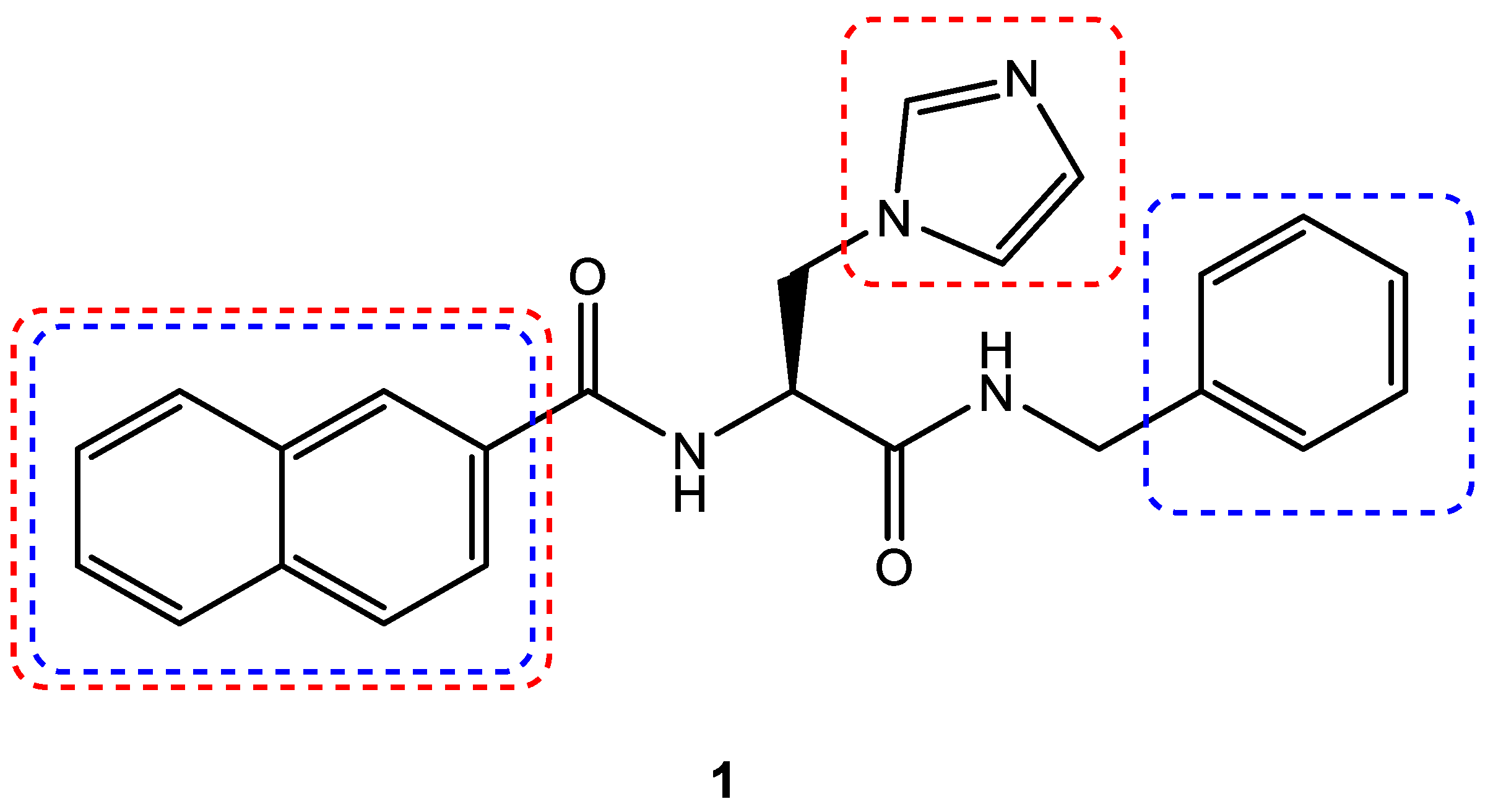
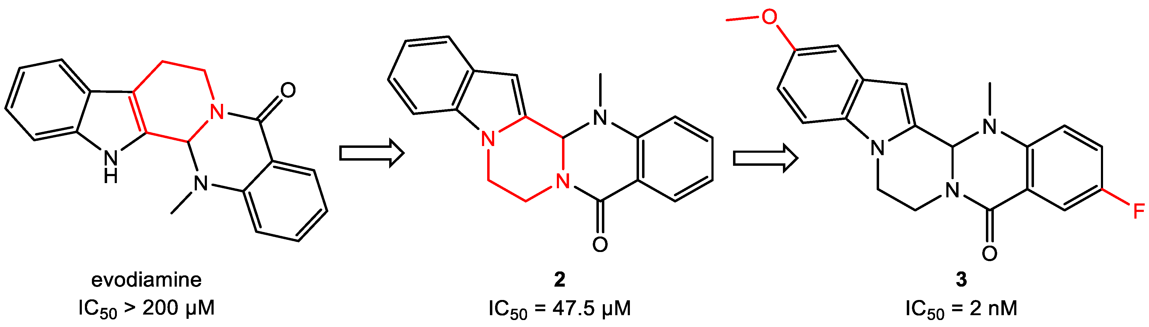
Scaffold hopping is particularly useful in optimising known ligands to improve their efficacy and ADME profile [276]. Blaquiere et al. discovered novel NF-κB inducing kinase (NIK) inhibitors with improved selectivity and pharmacokinetic properties using the scaffold hopping method. By replacing the oxepin ring in their previously discovered benzoxepine class NIK inhibitors with different cores, novel molecules with reduced nonoxidative metabolism (glutathione conjugation and amide hydrolysis) and thus reduced in vitro clearance were identified [277]. Scaffold hopping is also an effective strategy to optimise natural products with insufficient levels of activity and high structural complexity to increase their potency and synthetic accessibility. By changing the connectivity of the piperidine ring of natural product evodiamine, Wang and co-workers identified a novel indolopyrazinoquinazolinone scaffold 2 with anti-tumour properties, bringing the IC₅₀ value from over 200 µM to 47.5 µM when tested against HCT116 cells. Further structural optimisation resulted in a molecule 3 with an IC₅₀ value of 2 nM (Figure 11) [278].

4. De Novo and Fragment-Based Drug Design

De novo drug design allows the generation of novel molecules with new scaffolds, especially when majority of small molecule libraries have been exhausted for virtual screening. Before performing de novo drug design, the primary target constraints must be determined first. In SBDD where the structure of the receptor is known, molecular shapes, sub-molecular physical and chemical properties that are important for binding to the active site are extracted to derive shape constraints and interaction sites (normally divided into H-bonds, electrostatic and hydrophobic interactions). In LBDD, pharmacophore features can be used directly in a similarity design method or treated as interaction sites and generate a pseudo-receptor model [25].

Building blocks used for the generation of molecules can either be atoms or organic fragments. Early programs mainly used atom-based approach that is more likely to encounter issues with synthetic accessibility, but the molecules generated would be more diverse as all chemical space can be sampled. Newer programs use a fragment-based approach that is generally more synthetically feasible but the resulting molecules are relatively less diverse [279]. Furthermore, using fragments obtained by cleaving drug molecules had shown to generate ligands that are more likely to have drug-like properties [280]. Some examples of de novo/fragment-based drug design programs include LUDI [257], LigBuilder [281], ACFIS [282] and SEED [283].

Structure sampling can be carried out in various methods: linking, growing and lattice-based sampling. The linking approach links the building blocks that are positioned at the interaction sites with linker to form a complete molecule [257,284]. The growing approach starts off with one building block that is positioned at one of the interaction sites (starting point), then the structure grows from the starting point, trying to fit suitable interactions for the interaction sites as well as the regions of the receptor between interaction sites [285,286]. The lattice strategy places the binding pocket with lattice points and the ligands are formed from the lattice points that lie along the shortest path that connects the interaction points [287]. Once the molecules are generated, they can either be assessed with structure-based methods to predict the binding affinity, or with ligand-based methods where the molecules are compared to known active compounds. The ligands are then optimised until a promising drug candidate is produced.

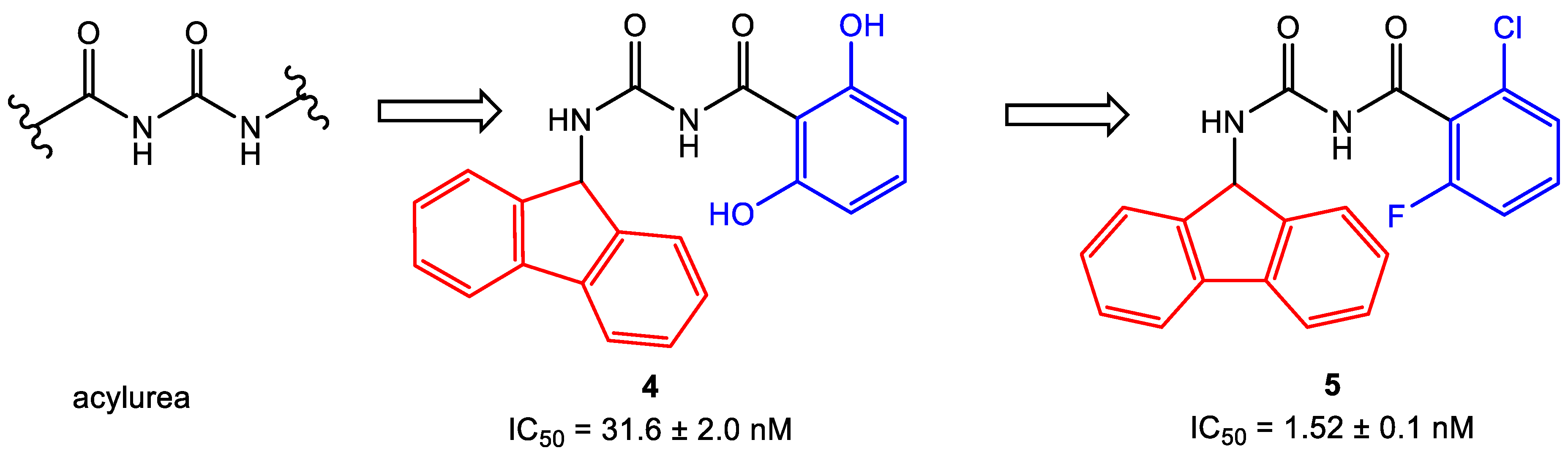
Ni and co-workers discovered a new class of Cyclophilin A (CypA) inhibitors using de novo drug design approach with LigBuilder 2.0. Analysis of existing CypA inhibitors shows that potent inhibitors contain an amide fragment as a linker that forms H-bond interactions with residues between the two sub-binding pockets. Using an acylurea linker as the starting point, new molecules are generated by growing structures from both ends of the structures to occupy the two sub-binding pockets of CypA. Out of the top 98 molecules that were generated, a common scaffold 4 was identified. Compound 4 was found to be potent and was further optimised based on SAR information to give 5 that was 20 times more potent (Figure 12) [288].

5. Hierarchical Virtual Screening (HLVS)

Both structure-based and ligand-based virtual screening methods have their own strengths and weaknesses. Structure-based methods are dependent on the availability of protein structures and it could be computationally demanding and time consuming for methods, such as MD and flexible molecular docking. Docking-based methods also demonstrate varying performance depending on the nature of the target binding sites [289]. Ligand-based screening methods on the other hand, rely heavily on the knowledge and information of active ligands and as a result are more biased towards the chemical scaffolds of available active compounds and generate less diverse results. Unlike docking studies where there are well established scoring functions used to approximate binding affinity and to rank molecules, pharmacophore methods lack a reliable and general scoring system. There can also be a lot of variations in models generated in ligand-based approaches, for example a slight difference in ligand selection in the training set could generate a very different QSAR model.

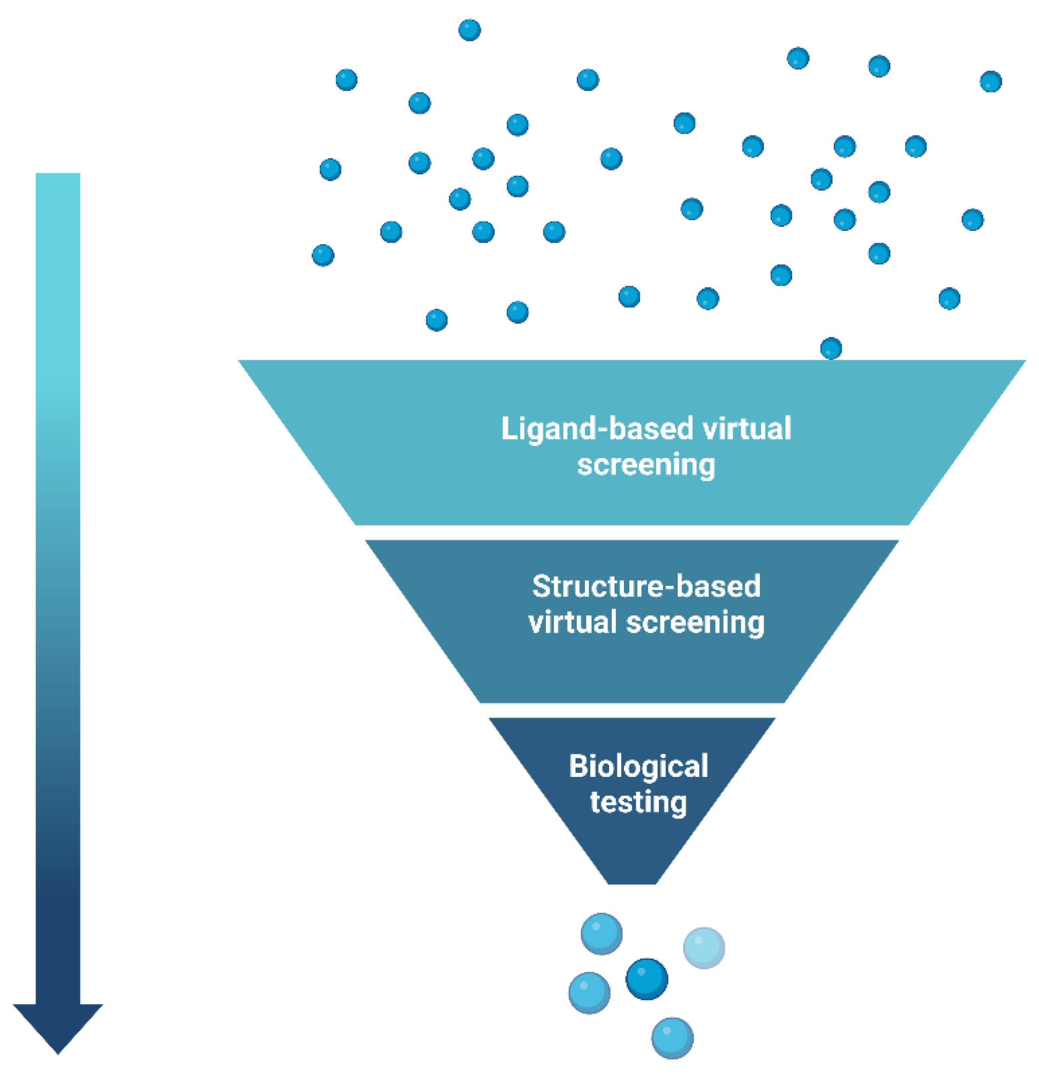
There are clear benefits to combine and integrate different approaches in CADD and the most common way is to use ligand- and structure-based methods in a sequential order, commonly known as hierarchical virtual screening (HLVS) (Figure 13). Generally, ligand-based filters are first applied because they are fast and less computationally expensive. Once the number of candidates is reduced, structure-based methods are applied to further filter inappropriate drug candidates before taking them for biological testing [290]. The hierarchical combination of pharmacophore modelling and molecular docking are the two most extensively employed methods in HLVS and there are numerous successful examples using this approach, such as the identification of matrix metalloproteinase 2 (MMP2) inhibitors by Di Pizio et al. [291] as well as the discovery of novel PKR-like endoplasmic reticulum kinase (PERK) inhibitors by Wang et al. [292].

6. Molecular Mechanical/Generalised Born Surface Area (MM-GBSA)

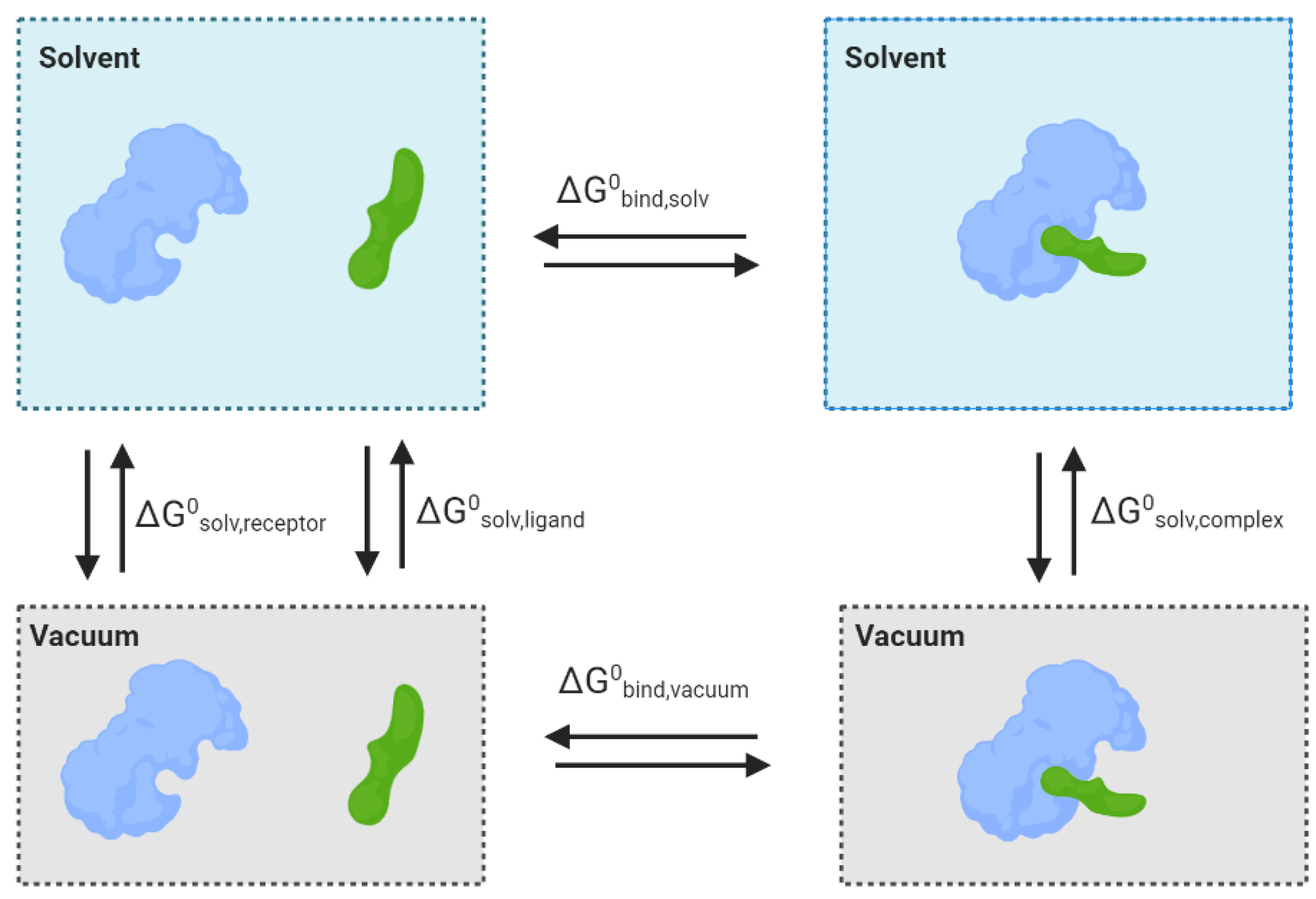
A more robust way to estimate the binding free energy of ligands to protein is to use the combined Molecular Mechanical/Generalised Born Surface Area (MM-GBSA) approach [293]. MM-GBSA is a force-field based method that computes the free energy of binding from the difference between the free energies of the protein, ligand, and the complex in solution. The free energy is calculated by using a combination of gas-phase molecular mechanics (MM) energy, electrostatic solvation energy (GB) and non-electrostatic contribution to solvation energy (SA). It provides a more accurate prediction because it can treat both the ligand and protein as flexible, allowing structural rearrangements required for the induced-fit pose. For the same reason, MM-GBSA is more computationally expensive compared to conventional docking studies, therefore they are generally implemented after a completed docking study to re-score selected ligands.

The total binding free energy ΔG_bind can be calculated using the following equation: [293]

$$\Delta {\mathrm{G}}_{\mathrm{bind}}={\mathrm{E}}_{\mathrm{complex}}-{\mathrm{E}}_{\mathrm{ligand}}-{ \mathrm{E}}_{\mathrm{receptor} }$$

(13)

where ${\mathrm{E}}_{\mathrm{complex}}$ is the energy of the optimised complex, ${\mathrm{E}}_{\mathrm{ligand}}$ and ${\mathrm{E}}_{\mathrm{receptor} }$ are the energy of the optimised free ligand and receptor, respectively. This equation can be further broken down into different components of the contributing energies:

$$\Delta {\mathrm{G}}_{\mathrm{bind}}=\Delta \mathrm{H} - \mathrm{T}\Delta \mathrm{S} =\Delta {\mathrm{E}}_{\mathrm{MM}}+\Delta {\mathrm{G}}_{sol}-\mathrm{T}\Delta \mathrm{S}$$

(14)

In which

$$\Delta {\mathrm{E}}_{\mathrm{MM}}=\Delta {\mathrm{E}}_{\mathrm{int}}+\Delta {\mathrm{E}}_{\mathrm{ele}}+\Delta {\mathrm{E}}_{\mathrm{vdW}}$$

(15)

$$\Delta {\mathrm{G}}_{sol}=\Delta {\mathrm{G}}_{PB/GB}+\Delta {\mathrm{G}}_{SA}$$

(16)

$$\Delta {\mathrm{G}}_{SA}= \mathsf{\gamma }·\mathrm{SASA}+b$$

(17)

where $\Delta {\mathrm{E}}_{MM}$ is the changes in the gas-phase molecular mechanics (MM) energy, including changes in the internal energy ($\Delta {\mathrm{E}}_{\mathrm{int}}$), electrostatic energy ($\Delta {\mathrm{E}}_{\mathrm{ele}}$) and vdW energy ($\Delta {\mathrm{E}}_{\mathrm{vdW}}$). $\Delta {\mathrm{G}}_{sol}$ is the sum of electrostatic solvation energy with polar contribution ($\Delta {\mathrm{G}}_{PB/GB}$) and non-polar contribution ($\Delta {\mathrm{G}}_{SA}$) between the solute and continuum solvent. $\Delta {\mathrm{G}}_{PB/GB}$ is calculated using either the Poisson-Boltzmann (PB) or generalised Born (GB) model. $\Delta {\mathrm{G}}_{SA}$ is estimated using the solvent-accessible surface area ($\mathrm{SASA}$), where $\mathsf{\gamma }$ is the surface tension constant and $b$ is a correction constant. The change in conformational entropy ($-\mathrm{T}\Delta \mathrm{S}$) is calculated by normal-mode analysis [294,295,296].

7. Molecular Dynamics

Molecular dynamics (MD) is an in silico simulation method based on molecular mechanics (MM), to study the individual particle motions of model systems over time [297]. MD can provide insights into biomolecular processes, such as protein folding, conformational changes, ligand binding and disassociation by simulating the interactions between atoms and molecules at an atomic level [298,299,300,301]. In the context of drug design, simulating the responses of proteins to various perturbations, including mutation [302], phosphorylation [303], protonation [304] and ligand binding [305], can be observed in well-established models, making MD a powerful tool in understanding the mechanisms for pathogenic or therapeutical processes. Since initially being applied in macromolecules [306], the application of MD simulation has been extensively developed, both in algorithms and force field parameters. A variety of MD software packages are available such as Gromacs [307], AMBER [308], Lammps [309], NAMD [310], CHARMM [311] and Desmond [312]. These mainstream programs for MD simulation share similar functionalities and have achieved high performance by utilising the compute power and speed of graphics processing units (GPUs). MD has been gradually accepted and is now widely used in pharmaceutical science especially with recent breakthroughs in both structural biology techniques (leading to a larger number of experimentally obtained protein structures) and computational hardware. Currently, MD simulation is integrated into the crucial pilot stages of drug discovery [313]. Two major usages of MD in recent novel drug design are: (1) to provide dynamic structural insights of biomolecules and (2) to provide precise energetic information of receptor–ligand complexes, key information in lead identification and lead optimisation.

In this context, MD provides valuable time-dependent information on drug targets and their ligands [314]. MD simulations calculate the position and motion of each atom at each timestep. With accurately controlled simulation conditions, MD can capture the binding processes in action, which are difficult to observe experimentally, provide the details, such as the path in which ligand slides into the binding pocket [315], how the protein–ligand intermediate state forms and evolves [316], giving explanation of the binding mechanism at atomic resolution.

For the ligand binding processes, MD always works hand-in-hand with molecular docking [317]. As previously mentioned, the flexibility of a protein structure is a fundamental factor in both protein biological function and the shape of a binding pocket. However, the initial protein structure used in SBDD are usually the state of the protein acquired from experimental methods, such as X-ray crystal diffraction or cryo-EM [313]. In reality, different states of the protein exist and the protein dynamics profoundly affect the binding process. Docking into a single static structure would likely retrieve only one subset of promising ligands.

There are two main hypotheses of the ligand recognition: conformational selection and induced fit mechanism, which may coexist in most cases [318]. MD combined with ensemble docking is one solution to address receptor flexibility by conducting simulations to explore the conformational space and select representative conformations as a receptor ensemble into following dockings. This method is usually integrated in virtual screening workflows to enrich the structural diversity of lead candidates and possible rational binding poses [319]. Many successful practices of MD-based ensemble docking have been published. Li et al. conducted unrestrained MD simulations on estrogen-related receptor α (ERRα) to obtain structural ensembles for a virtual screening scheme which combines similarity search and ensemble docking. Seven novel scaffolds different from known agonists with remarkable activity were identified [320]. Recently, machine learning (ML) methodologies were also introduced to boost ensemble docking both on ensemble optimisation [321] and ligand score aggregation [322]. On the other hand, methods based on the induced fit mechanism, are also powered by MD simulation. Induced fit docking methods that aim to address the flexibility issue in ligand binding have been successfully utilised in many drug discovery projects [323,324]. However, the poses sampling step of classic IFD still leaves worries on robustness and accuracy. Thus, MD is introduced into the upgraded methodology called IFD-MD to overcome these challenges [325]. Compared to the traditional IFD protocol, in IFD-MD, short MD simulations are first applied in the rescoring procedure to equilibrate the trial binding models, then metadynamic simulations [326,327] are conducted to assess the local stability. This new method showed promising outcome both in efficiency and accuracy. Zhang et al. discovered dual agonist with nanomolar affinity on both orexin-1 and orexin-2 receptors and performed comprehensive computational modelling studies, including IFD-MD and conventional MD to explore the binding interactions [328].

Another important objective of MD is capturing conformational changes, particularly those related to important functional processes. As these biomolecular processes usually take place on a larger timescale than conventional MD can sample (within reasonable time and computational cost), several sophisticated MD schemes such as steered MD (sMD) [329], accelerated MD (aMD) [330], replica-exchange MD (REMD) [331] and coarse-grained MD [332] were developed to overcome the barrier [333]. In drug discovery, MD is widely used to explain biomolecular mechanisms, such as drug resistance caused by mutations [302,334,335,336]. Compared to time-consuming experimental method, which only gives static structural information, MD can rapidly provide detailed explanations of the interactions between the ligand and the receptor, including drug–protein or protein–protein interactions and not only structural and dynamical information but also energetic insights. Many studies verified the feasibility of using MD simulations in studying virus resistance mechanisms especially on recent COVID-19 topics. Liu et al. performed an all-atom MD simulation and free energy calculation to explain the resistance mechanisms of SARS-COV-2 variants Delta and Lambda to bamlanivimab [337].

The design of drugs targeting allosteric sites is another application of MD [305,338]. Allosteric binding sites are usually not as obvious as orthosteric sites from experimentally obtained structures, often due to their reliance on ligand binding and the induced conformational changes [333]. The formation of cryptic pockets is also considered being adjusted by both mechanisms [339]: conformational selection based on the flexibility of the cryptic pockets first and then stabilised by ligand as induced fit [340]. MD simulations have been shown to be of great use in identifying cryptic binding pockets and distinguishing allosteric and orthosteric sites [341,342]. Mixed solvents MD simulation, which uses small molecules/fragments with water as probe, have been successfully applied to detect and characterise allosteric sites [343,344]. Zuzic et al. used molecular dynamics simulations with benzene probes to detect the cryptic pockets in the SARS-CoV-2 spike glycoprotein and successfully identified a potentially druggable cryptic [345].

Protein misfolding is also an important topic that MD method is deeply involved. Unlike regular protein folding processes which have plenty of well-established solutions including homology modelling [58,59,60] and ab initio modelling [70,71,72,73], the high-resolution dynamic misfolding procedures of intrinsically disordered proteins (IDPs) are extremely difficult to be investigated in experiments for their heterogeneity [346,347]. Among all the cases, the pathological misfolding and aggregation of Alzheimer’s disease (AD) related amyloid-β (Aβ) peptide and tau protein are the most pressing areas for novel therapeutic agent development. Man et al. evaluated the effects of MM force fields on amyloid peptide assembly based on the experimental observation [348,349]. Liu et al. constructed the Markov state model based on the microsecond time scale MD simulation to explore the mechanism of VQIVYK (PHF6) peptide for tau protein aggregation [350].

MD simulations can also contribute to lead candidates’ optimisation after the initial identification effort. Even though the structural information obtained by molecular docking provides insights into understanding the receptor-ligand interaction, the scoring functions suffered from their approximation in descripting desolvation, entropic penalties and conformational strains [351], leading to inaccurate energetic results in affinity prediction. The accurate evaluation of receptor–ligand interactions, along with the refinement of the binding complex structures, are needed, and they are becoming a standard protocol at the post-docking stage [352,353]. The purpose of MD optimisation is to fix clashes and stabilise and correct the binding complex, as well as to provide substantially accurate value of binding affinities by MD-based free energy calculations. Regular methods in this field consist of the alchemical approaches, such as thermodynamic integration (TI), free energy perturbation (FEP) [354,355,356,357] and endpoint approximation methods, such as molecular mechanics Poisson–Boltzmann (generalised Born) surface area (MM/PB(GB)SA) and linear interaction energy (LIE) (Figure 14) [295,358,359,360].

TI and FEP are theoretically rigorous methods with highly precise result. However, the sampling of the calculation requires a large amount of computing resources, and the system of computing is also limited because of the complicated simulations setup [361]. Usually, these methods are used to compare the free energy difference between two given systems with minor modifications, specifically, the lead optimisation process in drug design [362]. TI and FEP calculate the free energy difference between systems of similar chemical constitutions where the experimental data is not available. To accomplish the calculation, a thermodynamic cycle is introduced to connect the results from a series of TI calculations to experimental observables (Figure 15).

In this closed thermodynamic cycle, the free energy difference between two ligand binding ΔΔG can be calculated precisely as it is identical to ΔG₄–ΔG₃.

For two systems in TI approach, A and B, with potential energies $U_A$ and $U_B$, $\lambda$ is introduced as the coupling parameter with value between 1 and 0, the new potential energy function is defined as

$$U\left(\lambda \right)=U_A+\lambda \left(U_B-U_A\right)$$

(18)

In canonical ensemble, the partition function of the system is

$$Q\left(N,V,T,\lambda \right)={\displaystyle \sum }exp [-U\left(\lambda \right)/K_{B}T]$$

(19)

where $K_B$ is the Boltzmann constant, $NVT$ means constant number ($N$), volume ($V$), and temperature ($T$).

The free energy of the system is defined as

$$G_{\left(N,V,T,\lambda \right)}=-K_{B}Tln{Q}_{\left(N,V,T,\lambda \right)}$$

(20)

The free energy between A and B is calculated as

$$\mathsf{\Delta }G\left(A\to B\right)={\int }_0^{1}d\lambda \frac{\partial F\left(\lambda \right)}{\partial \lambda }={\int }_0^{1}d\lambda \frac{K_{B}T}{Q}\frac{\partial Q}{\partial \lambda }$$

(21)

$$\mathsf{\Delta }G\left(A\to B\right)={\int }_0^{1}d\lambda \frac{K_{B}T}{Q}{\displaystyle \sum }\frac{1}{K_{B}T}\mathit{exp} [-U\left(\lambda \right)/K_{B}T]\frac{\partial U\left(\lambda \right)}{\partial \lambda }$$

(22)

$$\mathsf{\Delta }G\left(A\to B\right)={\int }_0^{1}d\lambda \langle {\frac{\partial F\left(\lambda \right)}{\partial \lambda }\rangle }_{\lambda }$$

(23)

For FEP method, a series of small perturbations, in our cases minor chemical structural modifications, are conducted to link the starting and ending state. The derivation is similar to TI

$$G=-K_{B}TlnQ$$

(24)

$$\mathsf{\Delta }G\left(A\to B\right)=-K_{B}T\ln \left[\frac{Q_B}{Q_A}\right]$$

(25)

$$\mathsf{\Delta }G\left(A\to B\right)=-K_{B}Tln\left[\frac{\int e^{-U_B\left(\overrightarrow{q}\right)/K_{B}T}d\overrightarrow{q}}{Q_A}\right]$$

(26)

$$\mathsf{\Delta }G\left(A\to B\right)=-K_{B}T ln\langle e^{-\left(U_B\left(\overrightarrow{q}\right)-U_A\left(\overrightarrow{q}\right)\right)/K_{B}T}\rangle {}_A$$

(27)

where $\overrightarrow{q}$ is variable for coordinates and momentum.

Sophisticated solutions to drug discovery problems are provided by the application of TI and FEP. Nowadays most of the simulation packages support relative free energy simulations, including FEP plus within the Schrödinger suite [363], AMBER TI [364,365], CHARMM [366], Gromacs [367], Q open-source [368] MD package and so forth. Tang et al. utilised FEP to guide the discovery of novel D-amino acids oxidase inhibitors, with good consistency shown between bioassay results and the energy calculations [369]. Zou et al. developed a method for scaffold hopping transformations via alchemical free energy calculations, which broaden the usage of such approaches in lead modification and optimisation [370].

One issue that limits the utility of TI/FEP is the complicated set up for the system. Although the results of TI and FEP calculation are exact in theory, the accuracy is dependent on sampling/studying sufficient intermediate states that provide enough overlaps in each λ window. Different choices of λ are implemented, such as fixed value, slow growth and dynamic modified growth [371], improving the accuracy of the result, while also significantly increasing the computational cost. Even though GPU accelerated techniques have been applied in TI/FEP calculations [372], they are still not economically accessible for large datasets. Though MD software offered limited support to setup TI/FEP systems, much effort has been made to assist the preparation for TI/FEP calculations. Automated workflow tools, such as FESetup [373] for AMBER and Gromacs, PyAutoFEP [367] for Gromacs, FEPrepare [374] for NAMD, QligFEP [375] and QresFEP [376] for Q and many others [377,378,379] provide convenience for researchers to conduct alchemical free energy simulations in drug design.

MM/PB(GB)SA, as an endpoint method which depend on the sampling of the final states of the system, is a good trade-off for computational cost and accuracy in calculating the binding free energy [380]. The balanced performance makes it popular in broader utilities than the alchemical free energy methods [380,381,382].

As the system is always in solvent, $\mathsf{\Delta }{G}^0{}_{bind,solv}$ is almost impossible to calculate directly in explicit model because the majority of energetic contribution is made by the solvents instead of the complex, and the fluctuation of total energy is far beyond the binding energy [380]. Thus, the MM/PB(GB)SA also calculate through the thermodynamic cycle to avoid the problem (Figure 16).

$$\mathsf{\Delta }{G}^0{}_{bind,solv}=\mathsf{\Delta }{G}^0{}_{solv,complex}- \left(\mathsf{\Delta }{G}^0{}_{solv,ligand}-\mathsf{\Delta }{G}^0{}_{solv,receptor}\right)+\mathsf{\Delta }{G}^0{}_{bind,vacuum}$$

(28)

In which the total binding energy can be divided as solvation energy and gas phase MM energy ($\mathsf{\Delta }{G}^0{}_{bind,vacuum}$).

For the MM energy

$$\mathsf{\Delta }{G}^0{}_{bind,vacuum}=\mathsf{\Delta }{G}^0{}_{complex,vacuum}- \left(\mathsf{\Delta }{G}^0{}_{receptor,vacuum}+\mathsf{\Delta }{G}^0{}_{ligand,vacuum}\right)$$

(29)

$$=\mathsf{\Delta }{H}^0-T\mathsf{\Delta }{S}^0$$

(30)

$$=\left(\mathsf{\Delta }{E}^0{}_{int}+\mathsf{\Delta }{E}^0{}_{vdW}+\mathsf{\Delta }{E}^0{}_{ele}\right)-T\mathsf{\Delta }{S}^0$$

(31)

where $\mathsf{\Delta }{H}^0$ is the enthalpy changes in the gas-phase molecular mechanics (MM) energy which is calculated statistically based on the trajectories produced by MD, $\mathsf{\Delta }{E}^0{}_{int}$ stands for the internal energy including the bond, angle and dihedral, $\mathsf{\Delta }{E}^0{}_{vdW}$ for vdW energy and $\mathsf{\Delta }{E}^0{}_{ele}$ for electrostatic energy.$T\mathsf{\Delta }{S}^0$ is the contribution of entropy, which can be obtained by normal mode analysis, quasi-harmonic analysis or quasi-Gaussian approach.

As for the solvation energy, which consists of the electrostatic, vdW and cavity effects, can be represented as nonpolar and polar terms which is calculated in a different manner.

$$\mathsf{\Delta }{G}^0{}_{solv}=\mathsf{\Delta }{G}^0{}_{solv,vdw}+\mathsf{\Delta }{G}^0{}_{solv,cav}+\mathsf{\Delta }{G}^0{}_{solv,ele }=\mathsf{\Delta }{G}^0{}_{solv,nonpolar}+\mathsf{\Delta }{G}^0{}_{solv,polar}$$

(32)

In which the nonpolar energy $\mathsf{\Delta }{G}^0{}_{solv,nonpolar}$ is easy to estimate, the value is linearly proportional to the solvent-accessible surface area (SASA) because it is basically determined by the interaction with the first layer of solvents. The equation is as follows

$$\mathsf{\Delta }{G}^0{}_{solv,nonpolar}=\gamma SASA+b$$

(33)

where γ (0.00542 kcal/mol Å) and b (0.92 kcal/mol) are constants fitted to experimental data [383].

The polar solvation energy in implicit solvent $\mathsf{\Delta }{G}^0{}_{solv,polar}$ is estimated by Poisson–Boltzmann (PB) model or Generalised Born (GB) model. In the PB model, a solute is represented by an atomic-detail model as in a MM force field, while the solvent molecules and any dissolved electrolyte are treated as a structure-less continuum [308]. The continuum treatment represents the solute as a dielectric body whose shape is defined by atomic coordinates and atomic cavity radii [384]. The electrostatic field can be computed by solving the PB equation: [385]

$$\nabla • \left[\epsilon \left(r\right)\nabla \varphi \left(r\right)\right]=-4\pi \rho \left(r\right)-4\pi \lambda \left(r\right){\displaystyle \sum }_i{z}_i{c}_i\mathit{exp}(\frac{-z_i\varphi \left(r\right)}{K_{B}T})$$

(34)

where $\epsilon \left(r\right)$ is the dielectric constant, φ(r) is the electrostatic potential, $\rho \left(r\right)$ is the solute charge, $\lambda \left(r\right)$ is the Stern layer masking function, $z_i$ is the charge of ion type $i$, $c_i$ is the bulk number density of ion type $i$ far from the solute, $K_B$ is the Boltzmann constant, and $T$ is the temperature; the summation is over all different ion types. The salt term in the PB equation can be linearised when the Boltzmann factor is close to zero but in highly charged systems the PB equation cannot accurately describe the ionic interactions and correlation enhancement. In such systems, full nonlinear PB equation solvers are more appropriated [308]. The solvation free energy in PB model is represented as [386]

$$\mathsf{\Delta }{G}^0{}_{solv,polar}=\frac{1}{2}{\sum }_i{q}_i \left[{\varphi }_{\epsilon =80}\left(r_i\right)-{\varphi }_{\epsilon =1}\left(r_i\right)\right]$$

(35)

PB is an approach with standard numerical solution, obtaining results of better accuracy. However, the Poisson–Boltzmann equation needs to be solved every time the conformation changes, and hence the computational costs are relatively high in MD application [386].

The GB model is an alternative approach with reasonable approximates and good efficiency. Analytic generalised Born method is used to obtain the estimate of the electrostatic energy of solvation, each atom in molecule is represented as a sphere of radius $R_i$ with a charge $q_i$ in the centre, dielectric constant $\epsilon$ for solute and solvent are 1 and 80, respectively [294,387]. The equation is as below [381,388]

$$\begin{array}{l}\mathsf{\Delta }{G}^0{}_{solv,polar}=-\left(1-\frac{1}{\epsilon }\right){\displaystyle {\displaystyle \sum }_{i<j}}\frac{q_i{q}_j}{r_{ij}}-\frac{1}{2}\left(1-\frac{1}{\epsilon }\right){\displaystyle {\displaystyle \sum }_i}\frac{q_i{}^2}{a_i}\\ =-\frac{1}{2}{\displaystyle {\displaystyle \sum }_{ij}}\frac{q_i{q}_j}{f_{GB}\left(r_{ij},R_i,R_j\right)}\left(1-\frac{exp [-\kappa f_{GB}]}{\epsilon }\right)\end{array}$$

(36)

where $r_{ij}$ is the distance between atoms $i$ and $j$, the $R_i$ are the effective Born radii, and $f_{GB}$() is a certain smooth function of its arguments. The electrostatic screening effects of (monovalent) salt are incorporated via the Debye–Huckel screening parameter $\kappa$ [308].

The common representation of $f_{GB}\left(r_{ij},R_i,R_j\right)$ is [389]

$$f_{GB}=\sqrt{r^2{}_{ji}+R_i{R}_{j}exp(-r^2{}_{ij}/4R_i{R}_j)}$$

(37)

The advantages of MM/PB(GB)SA, including desired balance of accuracy/efficiency and the capability of computing absolute binding energy, give this method a much wider use in drug design. Current computational resources allow for the MM/PB(GB)SA to be implemented into the virtual screening workflow as a re-scoring tool to improve the hit rate [390]. MM/PB(GB)SA can also help to investigate the binding free energy of many two-component systems such as protein–ligand [391], protein–protein [350], protein–DNA systems [392] and many more. Moreover, binding free energy decomposition and the contribution of each residue, can be estimated in such a method, which gives key residue-specific information of the binding process [393,394].

8. QM/MM and DFT Approaches

Quantum mechanical (QM) and molecular mechanical (MM) calculations can be employed during the drug design process to explore the interaction between ligands and proteins and also how it is processed within the body (ADME). These calculations use a molecular descriptor approach allowing for prediction of ADME properties and modulation in the design process [395]. All of these factors are a consequence of the electronic interactions within a system. The use of molecular mechanics (MM) approaches has been discussed above. Quantum mechanical (QM) approaches provide more realistic results, often in agreement with experimental data, however at significantly greater computational cost when compared to MM [396]. QM approaches can be used to not only study the binding poses but also explore the energy landscape of natural processes or drug-receptor processes [397,398]. QM and MM approaches are used in two main ways to study ligand–protein interactions the first of which only utilises QM to analyse a small region of interest such as the binding site, while the second method also uses QM to analyse the region of interest while using the less computationally expensive MM approach to model the remainder of the system [397,398]. The application of pure Density Functional Theory (DFT) or ab initio work is limited due to the expensive computational cost, and as such it is limited to small systems, or for exploring derivable properties [399,400]. However, the application of the hybrid approach allows larger systems to be partitioned with the area of interest (i.e., the active site) being analysed with QM [401]. DFT is a well-established technique, and the experimental design needs to be in line with size, and property being explored for the system. DFT is computationally more efficient and accurate relative to QM (ab initio) methods. QM attempts to solve the Schrodinger equation to model the behaviour of the system and this is a non-trivial task for systems where N > 1 (where N is the number of electrons in the system). This can be highly accurate depending on the method employed (i.e., Moller–Plesset vs. Hartree Fock(HF)), however the equation cannot be fully solved as electron correlation effects $\left(E_{XC}\right)$ are unaccounted for. In contrast, DFT explores electronic behaviour of a molecule or system as function of the electronic density, with the energy being directly relatable [402]. This approach allows for much faster generation of a wavefunction to review and the accuracy is dependent on the functional applied. Recently, Bursch et al. provided a thorough review of the functionals and basis set selection for DFT application [403]. Commonly, for DFT in drug design setting, a hybrid functional (Equation (38)) is used

$$E_{XC}^{hybrid}=\alpha \left(E_X^{HF}-E_X^{GGA}\right)+E_C^{GGA}$$

(38)

In Equation (38) the $\alpha$ coefficient determines the amount of the exact exchange $(E_X^{HF})$ derived from first principles that is mixed with the semi-local exchange $(E_X^{GGA})$. This combined approach was proposed by Becke in 1993, with the first approach being a 50/50 mix for HF and semi-local E_X energies [404]. Since, the hybrid functional have grown significantly with an area of HF percentage amounts, commonly, it is between 20–30% [403]. The most commonly applied hybrid is the B3LYP functional containing a scalable 20% HF component [404,405,406]. Alongside a functional is a basis set, which provides numerical functionals for the molecular orbital shape and the occupational. Most commonly a split basis sets such as the 6-311 family is employed [407,408,409,410]. Albeit currently, functionals and basis sets of much higher complexity are being benchmarked and tested (i.e., Coupled-Cluster (CCSD(T), aug-cc-PVDZ, respectively) [411].

The hybrid approaches are more computationally efficient with the trade-off of reduced accuracy in regions away from the active site. However, these methods allow for entire system to be reviewed. QM/MM considers the whole system as conceptually two parts. The active/model region, which uses QM (DFT, commonly). The remaining region is studied using MM (force field approaches), with the boundary between both sites being the QM/MM interactions. The resultant energy of the system takes the form,

$$E_{sys}=E_{QM}+E_{MM}+E_{QM-MM}$$

(39)

Here, the system energy ($E_{sys}$) is the summative total of the QM, MM and interface region, respectively. It is obvious that the QM region is more computationally demanding, whilst the peripheries are much more efficient. This approach has been present since the 70s and its impact resulted in a Nobel prize being awarded to Karplus, Levitt and Warshel. [412,413] Since the two-part method, the QM/MM scheme has developed further to the currently more applied, which is our own n-layered Integrated molecular Orbital and Molecular mechanics (ONIOM) and comparative approaches. The ONIOM approach splits a system up to N-layers, with the inner layers closer to the active-site having an electronic density/energy calculated at a higher level of computational theory [401,414]. The MM analyses can be further enhanced by the addition of polarisation terms, solvating the system and even searching for excited states. A thorough review of the ONIOM is provided by Chung et al. and its vast application can be read there [401]. ONIOM has been applied in many computational packages, such as Gaussian and ORCA [415,416]. The boundary selection can be cumbersome, and considering the residue type and possible interactions it produces to influence the level of theory applied [401]. For drug design, ONIOM can be applied to provide energetic information in both structure- and ligand-based approaches. For structure-based approaches, the application of QM or QM/MM can be used to study enzymatic processes, when considering it as an outcome of energy [417,418]. At the core, the understanding of the Michaelis-Menten mechanistic scheme can be used to find rate constants between states [417]. In QM setting this is found by understanding the change in potential energy surface (PES) between states. This approach extends on how ligands interact with targets to understand how the PES is modified or overcome by generation or outcompeting of bonds [400,418,419,420,421]. Extending from PES alone, application analytical tools related to the properties of the wavefunction can be used to describe, modify and improve ligands. The use of frontier molecular orbital (FMO)s can be used to explore the electron donation ability of the ligand by analysis of the HOMO (highest occupied molecular orbital) and LUMO (lowest unoccupied molecular orbital), this can explore priori and postori energy of a ligand on binding [399]. Separately, the interactions present between ligand and receptor can be separated into energetic types to understand how bonding variations occur via R-group selection [399]. Other than ligand interactions and structure-based phenomena, DFT can be utilised to make predictions on binding affinities, pKa, IC₅₀, DFT-assisted QSAR, drug-interactions, delivery enhancement and ADME properties [401,414,422,423,424,425,426,427,428,429]. An example of ADME using DFT is the prediction of pKa [430]. DFT was used on the SAMPL6 bind test based on DFT alone and the error ranges were quite large (2–4 pKa units) [430]. Although, when using conceptual DFT (combining molecular descriptors with the DFT results) [431] in a machine learning model, predictions were improved and allowed for extension of the technique to be used for the prediction of non-acidic compounds as well. This approach overall lowered the errors to ~1.85 pKa units [432]. ADME predictions can also be made by utilising global reactivity descriptors, such as the Fukui Functions. This approach allows for the electron density of the molecule to be broken into neutral, positive or negative, which correlates to compounds that can cause electrophilic attack processes to aid in understanding toxicity [432,433]. Although less common in its use, QM/MM approaches have been pivotal in understanding many health burdens, such as, bacteria resistance, and HIV virus proteases process as two examples [422,434,435,436,437,438,439,440,441]. Noting its importance and success in many aspects, DFT or QM/MM approaches although currently under used, are growing in application due to improvement in computation resources. The application of QM or QM/MM can have ample benefit in drug design exploring how and why a process mechanistically occurs.

9. Conclusions

Recent advances in computational software and hardware have revolutionised the use of in silico methods in drug design, with access to high-performance computers allowing for more complex calculations and larger data sets to be feasibly processed. In this review, we have highlighted a range of in silico methods that are commonly used in the hit identification and lead optimisation stages of the drug design process, yet computational methods are also applied in other areas in the pipeline. Some examples include drug repurposing [442,443], protein–protein docking, de novo protein design, inverse docking [444], adverse events prediction, physiologically-based pharmacokinetic modelling, and guiding chemical synthesis [442,443].

In addition to classical CADD strategies, such as molecular docking and pharmacophore screening, more accurate and computationally expensive methods, such as MD, DFT, and MM/PB(GB)SA, are now routinely used to further analyse short-listed compounds to better predict binding interactions and docking energies, highlighting compounds which guide us into selecting and optimising the lead compound with the highest success rate.

With the rapid development in artificial intelligence, deep learning-based approaches in drug design have become a trending topic, and various of these strategies were developed for molecular docking [445,446], property prediction [447,448], compound retrosynthesis [449,450,451], de novo drug design [452,453] and many more. Although the benefits of incorporating machine learning elements have been highlighted in recent years, there are still certain limitations in these approaches. The training of an algorithm relies heavily on a large amount of data, and therefore the availability of a comprehensive and high-quality dataset directly impacts the performance of the algorithm. Many of the more complex and recent models which utilise machine learning capabilities lack transparency due to their “black box” nature, and the results are not always able to be rationally interpreted and applied, thus limiting the scope of their potential applications in rational drug discovery and design [454]. Nevertheless, the development machine learning based CADD methodologies will be one of the major focuses in the future to continue improving current strategies and to overcome existing challenging barriers in the drug discovery process.

References

- (FDA), U.S.F.D.A. The Drug Development Process. Available online: https://www.fda.gov/patients/learn-about-drug-and-device-approvals/drug-development-process (accessed on 2 February 2022).
- Wouters, O.J.; McKee, M.; Luyten, J. Estimated research and development investment needed to bring a new medicine to market, 2009–2018. Jama 2020, 323, 844–853. [Google Scholar] [CrossRef] [PubMed]
- Wong, C.H.; Siah, K.W.; Lo, A.W. Estimation of clinical trial success rates and related parameters. Biostatistics 2019, 20, 273–286. [Google Scholar] [CrossRef] [PubMed]
- DiMasi, J.A.; Grabowski, H.G.; Hansen, R.W. Innovation in the pharmaceutical industry: New estimates of R&D costs. J. Health Econ. 2016, 47, 20–33. [Google Scholar] [PubMed] [Green Version]
- DiMasi, J.A.; Hansen, R.W.; Grabowski, H.G. The price of innovation: New estimates of drug development costs. J. Health Econ. 2003, 22, 151–185. [Google Scholar] [CrossRef] [PubMed] [Green Version]
- Paul, S.M.; Mytelka, D.S.; Dunwiddie, C.T.; Persinger, C.C.; Munos, B.H.; Lindborg, S.R.; Schacht, A.L. How to improve R&D productivity: The pharmaceutical industry’s grand challenge. Nat. Rev. Drug Discov. 2010, 9, 203–214. [Google Scholar] [PubMed]
- Yang, Y.; Adelstein, S.J.; Kassis, A.I. Target discovery from data mining approaches. Drug Discov. Today 2009, 14, 147–154. [Google Scholar] [CrossRef]
- Moffat, J.G.; Rudolph, J.; Bailey, D. Phenotypic screening in cancer drug discovery—Past, present and future. Nat. Rev. Drug Discov. 2014, 13, 588–602. [Google Scholar] [CrossRef]
- Hart, C.P. Finding the target after screening the phenotype. Drug Discov. Today 2005, 10, 513–519. [Google Scholar] [CrossRef]
- Xia, X. Bioinformatics and drug discovery. Curr. Top. Med. Chem. 2017, 17, 1709–1726. [Google Scholar] [CrossRef] [Green Version]
- Morgan, P.; Brown, D.G.; Lennard, S.; Anderton, M.J.; Barrett, J.C.; Eriksson, U.; Fidock, M.; Hamren, B.; Johnson, A.; March, R.E. Impact of a five-dimensional framework on R&D productivity at AstraZeneca. Nat. Rev. Drug Discov. 2018, 17, 167–181. [Google Scholar]
- Morgan, P.; Van Der Graaf, P.H.; Arrowsmith, J.; Feltner, D.E.; Drummond, K.S.; Wegner, C.D.; Street, S.D.A. Can the flow of medicines be improved? Fundamental pharmacokinetic and pharmacological principles toward improving Phase II survival. Drug Discov. Today 2012, 17, 419–424. [Google Scholar] [CrossRef] [PubMed]
- Maple, H.J.; Garlish, R.A.; Rigau-Roca, L.; Porter, J.; Whitcombe, I.; Prosser, C.E.; Kennedy, J.; Henry, A.J.; Taylor, R.J.; Crump, M.P. Automated protein–ligand interaction screening by mass spectrometry. J. Med. Chem. 2012, 55, 837–851. [Google Scholar] [CrossRef] [PubMed]
- Dalvit, C. NMR methods in fragment screening: Theory and a comparison with other biophysical techniques. Drug Discov. Today 2009, 14, 1051–1057. [Google Scholar] [CrossRef] [PubMed]
- O’Reilly, M.; Cleasby, A.; Davies, T.G.; Hall, R.J.; Ludlow, R.F.; Murray, C.W.; Tisi, D.; Jhoti, H. Crystallographic screening using ultra-low-molecular-weight ligands to guide drug design. Drug Discov. Today 2019, 24, 1081–1086. [Google Scholar] [CrossRef]
- Shuker, S.B.; Hajduk, P.J.; Meadows, R.P.; Fesik, S.W. Discovering high-affinity ligands for proteins: SAR by NMR. Science 1996, 274, 1531–1534. [Google Scholar] [CrossRef]
- Madsen, D.; Azevedo, C.; Micco, I.; Petersen, L.K.; Hansen, N.J.V. Chapter Four—An overview of DNA-encoded libraries: A versatile tool for drug discovery. In Progress in Medicinal Chemistry; Witty, D.R., Cox, B., Eds.; Elsevier: Amsterdam, The Netherlands, 2020; Volume 59, pp. 181–249. [Google Scholar]
- Macarron, R.; Banks, M.N.; Bojanic, D.; Burns, D.J.; Cirovic, D.A.; Garyantes, T.; Green, D.V.S.; Hertzberg, R.P.; Janzen, W.P.; Paslay, J.W.; et al. Impact of high-throughput screening in biomedical research. Nat. Rev. Drug Discov. 2011, 10, 188–195. [Google Scholar] [CrossRef]
- Shoichet, B.K. Virtual screening of chemical libraries. Nature 2004, 432, 862–865. [Google Scholar] [CrossRef] [Green Version]
- Kola, I.; Landis, J. Can the pharmaceutical industry reduce attrition rates? Nat. Rev. Drug Discov. 2004, 3, 711–716. [Google Scholar] [CrossRef]
- Bajorath, J. Integration of virtual and high-throughput screening. Nat. Rev. Drug Discov. 2002, 1, 882–894. [Google Scholar] [CrossRef]
- Karplus, M.; Petsko, G.A. Molecular dynamics simulations in biology. Nature 1990, 347, 631–639. [Google Scholar] [CrossRef]
- Shoichet, B.K.; McGovern, S.L.; Wei, B.; Irwin, J.J. Lead discovery using molecular docking. Curr. Opin. Chem. Biol. 2002, 6, 439–446. [Google Scholar] [CrossRef] [PubMed]
- Chen, Y.; Shoichet, B.K. Molecular docking and ligand specificity in fragment-based inhibitor discovery. Nat. Chem. Biol. 2009, 5, 358–364. [Google Scholar] [CrossRef] [PubMed] [Green Version]
- Schneider, G.; Fechner, U. Computer-based de novo design of drug-like molecules. Nat. Rev. Drug Discov. 2005, 4, 649–663. [Google Scholar] [CrossRef] [PubMed]
- EMBL-EBI UniProtKB/TrEMBL Protein Database Release 2022_02 Statistics. Available online: https://www.ebi.ac.uk/uniprot/TrEMBLstats (accessed on 27 July 2022).
- Bank, R.P.D. PDB Statistics: Overall Growth of Released Structures Per Year. Available online: https://www.rcsb.org/stats/growth/growth-released-structures (accessed on 27 July 2022).
- Consortium, U. UniProt: A hub for protein information. Nucleic Acids Res. 2015, 43, D204–D212. [Google Scholar] [CrossRef] [PubMed] [Green Version]
- Altschul, S.F.; Madden, T.L.; Schäffer, A.A.; Zhang, J.; Zhang, Z.; Miller, W.; Lipman, D.J. Gapped BLAST and PSI-BLAST: A new generation of protein database search programs. Nucleic Acids Res. 1997, 25, 3389–3402. [Google Scholar] [CrossRef] [Green Version]
- Bernstein, F.C.; Koetzle, T.F.; Williams, G.J.; Meyer Jr, E.F.; Brice, M.D.; Rodgers, J.R.; Kennard, O.; Shimanouchi, T.; Tasumi, M. The Protein Data Bank: A computer-based archival file for macromolecular structures. Eur. J. Biochem. 1977, 80, 319–324. [Google Scholar] [CrossRef]
- Sánchez, R.; Šali, A. Comparative protein structure modeling as an optimization problem. J. Mol. Struct. THEOCHEM 1997, 398–399, 489–496. [Google Scholar] [CrossRef]
- Madeira, F.; Park, Y.M.; Lee, J.; Buso, N.; Gur, T.; Madhusoodanan, N.; Basutkar, P.; Tivey, A.R.; Potter, S.C.; Finn, R.D. The EMBL-EBI search and sequence analysis tools APIs in 2019. Nucleic Acids Res. 2019, 47, W636–W641. [Google Scholar] [CrossRef] [Green Version]
- Needleman, S.B.; Wunsch, C.D. A general method applicable to the search for similarities in the amino acid sequence of two proteins. J. Mol. Biol. 1970, 48, 443–453. [Google Scholar] [CrossRef]
- Bellman, R. Dynamic programming. Science 1966, 153, 34–37. [Google Scholar] [CrossRef]
- Smith, T.F.; Waterman, M.S. Identification of common molecular subsequences. J. Mol. Biol. 1981, 147, 195–197. [Google Scholar] [CrossRef] [PubMed]
- Thompson, J.D.; Gibson, T.J.; Higgins, D.G. Multiple sequence alignment using ClustalW and ClustalX. Curr. Protoc. Bioinform. 2003, 1, 2–3. [Google Scholar] [CrossRef]
- Notredame, C.; Higgins, D.G.; Heringa, J. T-Coffee: A novel method for fast and accurate multiple sequence alignment. J. Mol. Biol. 2000, 302, 205–217. [Google Scholar] [CrossRef] [Green Version]
- Edgar, R.C. MUSCLE: Multiple sequence alignment with high accuracy and high throughput. Nucleic Acids Res. 2004, 32, 1792–1797. [Google Scholar] [CrossRef] [Green Version]
- Pei, J.; Kim, B.H.; Grishin, N.V. PROMALS3D: A tool for multiple protein sequence and structure alignments. Nucleic Acids Res. 2008, 36, 2295–2300. [Google Scholar] [CrossRef] [PubMed]
- Garibsingh, R.-A.A.; Otte, N.J.; Ndaru, E.; Colas, C.; Grewer, C.; Holst, J.; Schlessinger, A. Homology Modeling Informs Ligand Discovery for the Glutamine Transporter ASCT2. Front. Chem. 2018, 6, 279. [Google Scholar] [CrossRef] [PubMed] [Green Version]
- Choi, Y.; Deane, C.M. FREAD revisited: Accurate loop structure prediction using a database search algorithm. Proteins Struct. Funct. Bioinform. 2010, 78, 1431–1440. [Google Scholar] [CrossRef] [PubMed]
- Yang, M.; Simon, R.; MacKerell Jr, A.D. Conformational preference of serogroup B Salmonella O polysaccharide in presence and absence of the monoclonal antibody Se155–4. J. Phys. Chem. B 2017, 121, 3412–3423. [Google Scholar] [CrossRef] [Green Version]
- Stein, A.; Kortemme, T. Improvements to robotics-inspired conformational sampling in rosetta. PLoS ONE 2013, 8, e63090. [Google Scholar] [CrossRef] [Green Version]
- Guaitoli, G.; Raimondi, F.; Gilsbach, B.K.; Gómez-Llorente, Y.; Deyaert, E.; Renzi, F.; Li, X.; Schaffner, A.; Jagtap, P.K.A.; Boldt, K. Structural model of the dimeric Parkinson’s protein LRRK2 reveals a compact architecture involving distant interdomain contacts. Proc. Natl. Acad. Sci. USA 2016, 113, E4357–E4366. [Google Scholar] [CrossRef] [Green Version]
- Wang, Q.; Canutescu, A.A.; Dunbrack Jr, R.L. SCWRL and MolIDE: Computer programs for side-chain conformation prediction and homology modeling. Nat. Protoc. 2008, 3, 1832. [Google Scholar] [CrossRef] [PubMed]
- Moro, S.; Deflorian, F.; Bacilieri, M.; Spalluto, G. Ligand-based homology modeling as attractive tool to inspect GPCR structural plasticity. Curr. Pharm. Des. 2006, 12, 2175–2185. [Google Scholar] [CrossRef] [PubMed]
- Gacasan, S.B.; Baker, D.L.; Parrill, A.L. G protein-coupled receptors: The evolution of structural insight. AIMS Biophys. 2017, 4, 491. [Google Scholar] [CrossRef] [PubMed]
- Rodríguez, D.; Ranganathan, A.; Carlsson, J. Strategies for improved modeling of GPCR-drug complexes: Blind predictions of serotonin receptors bound to ergotamine. J. Chem. Inf. Model. 2014, 54, 2004–2021. [Google Scholar] [CrossRef] [PubMed]
- Kołaczkowski, M.; Bucki, A.; Feder, M.; Pawłowski, M. Ligand-optimized homology models of D1 and D2 dopamine receptors: Application for virtual screening. J. Chem. Inf. Model. 2013, 53, 638–648. [Google Scholar] [CrossRef]
- Cichero, E.; Menozzi, G.; Guariento, S.; Fossa, P. Ligand-based homology modelling of the human CB2 receptor SR144528 antagonist binding site: A computational approach to explore the 1, 5-diaryl pyrazole scaffold. MedChemComm 2015, 6, 1978–1986. [Google Scholar] [CrossRef]
- Evers, A.; Klebe, G. Successful virtual screening for a submicromolar antagonist of the neurokinin-1 receptor based on a ligand-supported homology model. J. Med. Chem. 2004, 47, 5381–5392. [Google Scholar] [CrossRef]
- Freyd, T.; Warszycki, D.; Mordalski, S.; Bojarski, A.J.; Sylte, I.; Gabrielsen, M. Ligand-guided homology modelling of the GABAB2 subunit of the GABAB receptor. PLoS ONE 2017, 12, e0173889. [Google Scholar] [CrossRef] [Green Version]
- Schaller, D.; Hagenow, S.; Stark, H.; Wolber, G. Ligand-guided homology modeling drives identification of novel histamine H3 receptor ligands. PLoS ONE 2019, 14, e0218820. [Google Scholar] [CrossRef] [Green Version]
- Hameduh, T.; Haddad, Y.; Adam, V.; Heger, Z. Homology modeling in the time of collective and artificial intelligence. Comput. Struct. Biotechnol. J. 2020, 18, 3494–3506. [Google Scholar] [CrossRef]
- Bonneau, R.; Strauss, C.E.; Rohl, C.A.; Chivian, D.; Bradley, P.; Malmström, L.; Robertson, T.; Baker, D. De novo prediction of three-dimensional structures for major protein families. J. Mol. Biol. 2002, 322, 65–78. [Google Scholar] [CrossRef] [PubMed]
- Goodsell, D.S.; Olson, A.J. Structural Symmetry and Protein Function. Annu. Rev. Biophys. Biomol. Struct. 2000, 29, 105–153. [Google Scholar] [CrossRef] [PubMed]
- Anfinsen, C.B. Principles that govern the folding of protein chains. Science 1973, 181, 223–230. [Google Scholar] [CrossRef] [PubMed] [Green Version]
- Klepeis, J.L.; Floudas, C.A. ASTRO-FOLD: A Combinatorial and Global Optimization Framework for Ab Initio Prediction of Three-Dimensional Structures of Proteins from the Amino Acid Sequence. Biophys. J. 2003, 85, 2119–2146. [Google Scholar] [CrossRef] [PubMed] [Green Version]
- Subramani, A.; Wei, Y.; Floudas, C.A. ASTRO-FOLD 2.0: An Enhanced Framework for Protein Structure Prediction. AIChE J 2012, 58, 1619–1637. [Google Scholar] [CrossRef] [PubMed] [Green Version]
- Ołdziej, S.; Czaplewski, C.; Liwo, A.; Chinchio, M.; Nanias, M.; Vila, J.; Khalili, M.; Arnautova, Y.; Jagielska, A.; Makowski, M.O. Physics-based protein-structure prediction using a hierarchical protocol based on the UNRES force field: Assessment in two blind tests. Proc. Natl. Acad. Sci. USA 2005, 102, 7547–7552. [Google Scholar] [CrossRef] [Green Version]
- Bowie, J.U.; Eisenberg, D. An evolutionary approach to folding small alpha-helical proteins that uses sequence information and an empirical guiding fitness function. Proc. Natl. Acad. Sci. USA 1994, 91, 4436–4440. [Google Scholar] [CrossRef] [Green Version]
- Hart, T.N.; Read, R.J. A multiple-start Monte Carlo docking method. Proteins Struct. Funct. Bioinform. 1992, 13, 206–222. [Google Scholar] [CrossRef]
- Shim, J.; MacKerell Jr, A.D. Computational ligand-based rational design: Role of conformational sampling and force fields in model development. Medchemcomm 2011, 2, 356–370. [Google Scholar] [CrossRef] [Green Version]
- Alford, R.F.; Leaver-Fay, A.; Jeliazkov, J.R.; O′Meara, M.J.; DiMaio, F.P.; Park, H.; Shapovalov, M.V.; Renfrew, P.D.; Mulligan, V.K.; Kappel, K.; et al. The Rosetta All-Atom Energy Function for Macromolecular Modeling and Design. J. Chem. Theory Comput. 2017, 13, 3031–3048. [Google Scholar] [CrossRef]
- Roy, A.; Kucukural, A.; Zhang, Y. I-TASSER: A unified platform for automated protein structure and function prediction. Nat. Protoc. 2010, 5, 725–738. [Google Scholar] [CrossRef] [PubMed]
- Xu, D.; Zhang, J.; Roy, A.; Zhang, Y. Automated protein structure modeling in CASP9 by I-TASSER pipeline combined with QUARK-based ab initio folding and FG-MD-based structure refinement. Proteins Struct. Funct. Bioinform. 2011, 79, 147–160. [Google Scholar] [CrossRef] [PubMed] [Green Version]
- Mistry, J.; Chuguransky, S.; Williams, L.; Qureshi, M.; Salazar Gustavo, A.; Sonnhammer, E.L.L.; Tosatto, S.C.E.; Paladin, L.; Raj, S.; Richardson, L.J.; et al. Pfam: The protein families database in 2021. Nucleic Acids Res. 2021, 49, D412–D419. [Google Scholar] [CrossRef] [PubMed]
- Marks, D.S.; Colwell, L.J.; Sheridan, R.; Hopf, T.A.; Pagnani, A.; Zecchina, R.; Sander, C. Protein 3D structure computed from evolutionary sequence variation. PLoS ONE 2011, 6, e28766. [Google Scholar] [CrossRef] [PubMed] [Green Version]
- Tetchner, S.; Kosciolek, T.; Jones, D.T. Opportunities and limitations in applying coevolution-derived contacts to protein structure prediction. Bio-Algorithms Med. Syst. 2014, 10, 243–254. [Google Scholar] [CrossRef]
- Xu, J. Distance-based protein folding powered by deep learning. Proc. Natl. Acad. Sci. USA 2019, 116, 16856–16865. [Google Scholar] [CrossRef] [Green Version]
- Uziela, K.; Menéndez Hurtado, D.; Shu, N.; Wallner, B.; Elofsson, A. ProQ3D: Improved model quality assessments using deep learning. Bioinformatics 2017, 33, 1578–1580. [Google Scholar] [CrossRef] [Green Version]
- Zheng, W.; Li, Y.; Zhang, C.; Zhou, X.; Pearce, R.; Bell, E.W.; Huang, X.; Zhang, Y. Protein structure prediction using deep learning distance and hydrogen-bonding restraints in CASP14. Proteins Struct. Funct. Bioinform. 2021, 89, 1734–1751. [Google Scholar] [CrossRef]
- Du, Z.; Su, H.; Wang, W.; Ye, L.; Wei, H.; Peng, Z.; Anishchenko, I.; Baker, D.; Yang, J. The trRosetta server for fast and accurate protein structure prediction. Nat. Protoc. 2021, 16, 5634–5651. [Google Scholar] [CrossRef]
- Baek, M.; DiMaio, F.; Anishchenko, I.; Dauparas, J.; Ovchinnikov, S.; Lee, G.R.; Wang, J.; Cong, Q.; Kinch, L.N.; Schaeffer, R.D. Accurate prediction of protein structures and interactions using a three-track neural network. Science 2021, 373, 871–876. [Google Scholar] [CrossRef]
- Senior, A.W.; Evans, R.; Jumper, J.; Kirkpatrick, J.; Sifre, L.; Green, T.; Qin, C.; Žídek, A.; Nelson, A.W.; Bridgland, A. Protein structure prediction using multiple deep neural networks in the 13th Critical Assessment of Protein Structure Prediction (CASP13). Proteins Struct. Funct. Bioinform. 2019, 87, 1141–1148. [Google Scholar] [CrossRef] [PubMed]
- Zemla, A. LGA: A method for finding 3D similarities in protein structures. Nucleic Acids Res. 2003, 31, 3370–3374. [Google Scholar] [CrossRef] [Green Version]
- Antoniak, A.; Biskupek, I.; Bojarski, K.K.; Czaplewski, C.; Giełdoń, A.; Kogut, M.; Kogut, M.M.; Krupa, P.; Lipska, A.G.; Liwo, A. Modeling protein structures with the coarse-grained UNRES force field in the CASP14 experiment. J. Mol. Graph. Model. 2021, 108, 108008. [Google Scholar] [CrossRef] [PubMed]
- Varadi, M.; Anyango, S.; Deshpande, M.; Nair, S.; Natassia, C.; Yordanova, G.; Yuan, D.; Stroe, O.; Wood, G.; Laydon, A. AlphaFold Protein Structure Database: Massively expanding the structural coverage of protein-sequence space with high-accuracy models. Nucleic Acids Res. 2022, 50, D439–D444. [Google Scholar] [CrossRef] [PubMed]
- Hooft, R.W.; Vriend, G.; Sander, C.; Abola, E.E. Errors in protein structures. Nature 1996, 381, 272. [Google Scholar] [CrossRef] [PubMed]
- Ramachandran, G.T.; Sasisekharan, V. Conformation of polypeptides and proteins. In Advances in Protein Chemistry; Elsevier: Amsterdam, The Netherlands, 1968; Volume 23, pp. 283–437. [Google Scholar]
- Eisenberg, D.; Lüthy, R.; Bowie, J.U. [20] VERIFY3D: Assessment of protein models with three-dimensional profiles. In Methods in Enzymology; Elsevier: Amsterdam, The Netherlands, 1997; Volume 277, pp. 396–404. [Google Scholar]
- Chen, V.B.; Arendall, W.B.; Headd, J.J.; Keedy, D.A.; Immormino, R.M.; Kapral, G.J.; Murray, L.W.; Richardson, J.S.; Richardson, D.C. MolProbity: All-atom structure validation for macromolecular crystallography. Acta Crystallogr. Sect. D Biol. Crystallogr. 2010, 66, 12–21. [Google Scholar] [CrossRef] [Green Version]
- Williams, C.J.; Headd, J.J.; Moriarty, N.W.; Prisant, M.G.; Videau, L.L.; Deis, L.N.; Verma, V.; Keedy, D.A.; Hintze, B.J.; Chen, V.B. MolProbity: More and better reference data for improved all-atom structure validation. Protein Sci. 2018, 27, 293–315. [Google Scholar] [CrossRef]
- Weichenberger, C.X.; Sippl, M.J. NQ-Flipper: Recognition and correction of erroneous asparagine and glutamine side-chain rotamers in protein structures. Nucleic Acids Res. 2007, 35 (Suppl. S2), W403–W406. [Google Scholar] [CrossRef] [Green Version]
- Rochira, W.; Agirre, J. Iris: Interactive all-in-one graphical validation of 3D protein model iterations. Protein Sci. 2021, 30, 93–107. [Google Scholar] [CrossRef]
- Bienert, S.; Waterhouse, A.; De Beer, T.A.; Tauriello, G.; Studer, G.; Bordoli, L.; Schwede, T. The SWISS-MODEL Repository—New features and functionality. Nucleic Acids Res. 2017, 45, D313–D319. [Google Scholar] [CrossRef] [Green Version]
- Bond, P.S.; Wilson, K.S.; Cowtan, K.D. Predicting protein model correctness in Coot using machine learning. Acta Crystallogr. Sect. D Struct. Biol. 2020, 76, 713–723. [Google Scholar] [CrossRef] [PubMed]
- Emsley, P.; Lohkamp, B.; Scott, W.G.; Cowtan, K. Features and development of Coot. Acta Crystallogr. Sect. D Biol. Crystallogr. 2010, 66, 486–501. [Google Scholar] [CrossRef] [PubMed] [Green Version]
- Emsley, P.; Cowtan, K. Coot: Model-building tools for molecular graphics. Acta Crystallogr. Sect. D Biol. Crystallogr. 2004, 60, 2126–2132. [Google Scholar] [CrossRef] [Green Version]
- O’Reilly, F.J.; Rappsilber, J. Cross-linking mass spectrometry: Methods and applications in structural, molecular and systems biology. Nat. Struct. Mol. Biol. 2018, 25, 1000–1008. [Google Scholar] [CrossRef] [PubMed] [Green Version]
- Liu, Y.L.; Lindert, S.; Zhu, W.; Wang, K.; McCammon, J.A.; Oldfield, E. Taxodione and arenarone inhibit farnesyl diphosphate synthase by binding to the isopentenyl diphosphate site. Proc. Natl. Acad. Sci. USA 2014, 111, E2530-9. [Google Scholar] [CrossRef] [Green Version]
- Trott, O.; Olson, A.J. AutoDock Vina: Improving the speed and accuracy of docking with a new scoring function, efficient optimization, and multithreading. J. Comput. Chem. 2010, 31, 455–461. [Google Scholar] [CrossRef] [PubMed] [Green Version]
- Verdonk, M.L.; Cole, J.C.; Hartshorn, M.J.; Murray, C.W.; Taylor, R.D. Improved protein–ligand docking using GOLD. Proteins Struct. Funct. Bioinform. 2003, 52, 609–623. [Google Scholar] [CrossRef] [PubMed]
- Friesner, R.A.; Banks, J.L.; Murphy, R.B.; Halgren, T.A.; Klicic, J.J.; Mainz, D.T.; Repasky, M.P.; Knoll, E.H.; Shelley, M.; Perry, J.K. Glide: A new approach for rapid, accurate docking and scoring. 1. Method and assessment of docking accuracy. J. Med. Chem. 2004, 47, 1739–1749. [Google Scholar] [CrossRef]
- Halgren, T.A.; Murphy, R.B.; Friesner, R.A.; Beard, H.S.; Frye, L.L.; Pollard, W.T.; Banks, J.L. Glide: A new approach for rapid, accurate docking and scoring. 2. Enrichment factors in database screening. J. Med. Chem. 2004, 47, 1750–1759. [Google Scholar] [CrossRef]
- Grosdidier, A.; Zoete, V.; Michielin, O. SwissDock, a protein-small molecule docking web service based on EADock DSS. Nucleic Acids Res. 2011, 39 (Suppl. S2), W270–W277. [Google Scholar] [CrossRef] [Green Version]
- Santos, K.B.; Guedes, I.A.; Karl, A.L.; Dardenne, L.E. Highly flexible ligand docking: Benchmarking of the DockThor program on the LEADS-PEP protein–peptide data set. J. Chem. Inf. Model. 2020, 60, 667–683. [Google Scholar] [CrossRef] [PubMed]
- Liu, Y.; Grimm, M.; Dai, W.-t.; Hou, M.-c.; Xiao, Z.-X.; Cao, Y. CB-Dock: A web server for cavity detection-guided protein–ligand blind docking. Acta Pharmacol. Sin. 2020, 41, 138–144. [Google Scholar] [CrossRef] [PubMed]
- Chemical Computing Group Inc. Molecular Operating Environment (MOE); Chemical Computing Group Inc.: Montreal, QC, Canada, 2022. [Google Scholar]
- Sastry, G.M.; Adzhigirey, M.; Day, T.; Annabhimoju, R.; Sherman, W. Protein and ligand preparation: Parameters, protocols, and influence on virtual screening enrichments. J. Comput. Aided Mol. Des. 2013, 27, 221–234. [Google Scholar] [CrossRef] [PubMed]
- Lengauer, T.; Rarey, M. Computational methods for biomolecular docking. Curr. Opin. Struct. Biol. 1996, 6, 402–406. [Google Scholar] [CrossRef]
- Fischer, E. Einfluss der Configuration auf die Wirkung der Enzyme. Ber. Der Dtsch. Chem. Ges. 1894, 27, 2985–2993. [Google Scholar] [CrossRef] [Green Version]
- López, G.; Valencia, A.; Tress, M.L. firestar—Prediction of functionally important residues using structural templates and alignment reliability. Nucleic Acids Res. 2007, 35 (Suppl. S2), W573–W577. [Google Scholar] [CrossRef] [Green Version]
- Wass, M.N.; Kelley, L.A.; Sternberg, M.J. 3DLigandSite: Predicting ligand-binding sites using similar structures. Nucleic Acids Res. 2010, 38 (Suppl. S2), W469–W473. [Google Scholar] [CrossRef] [Green Version]
- Toti, D.; Viet Hung, L.; Tortosa, V.; Brandi, V.; Polticelli, F. LIBRA-WA: A web application for ligand binding site detection and protein function recognition. Bioinformatics 2018, 34, 878–880. [Google Scholar] [CrossRef] [Green Version]
- Viet Hung, L.; Caprari, S.; Bizai, M.; Toti, D.; Polticelli, F. Libra: Ligand binding site recognition application. Bioinformatics 2015, 31, 4020–4022. [Google Scholar] [CrossRef]
- Laskowski, R.A. SURFNET: A program for visualizing molecular surfaces, cavities, and intermolecular interactions. J. Mol. Graph. 1995, 13, 323–330. [Google Scholar] [CrossRef]
- Halgren, T. New method for fast and accurate binding-site identification and analysis. Chem. Biol. Drug Des. 2007, 69, 146–148. [Google Scholar] [CrossRef] [PubMed]
- Halgren, T.A. Identifying and characterizing binding sites and assessing druggability. J. Chem. Inf. Model. 2009, 49, 377–389. [Google Scholar] [CrossRef] [PubMed]
- Brenke, R.; Kozakov, D.; Chuang, G.-Y.; Beglov, D.; Hall, D.; Landon, M.R.; Mattos, C.; Vajda, S. Fragment-based identification of druggable ‘hot spots’ of proteins using Fourier domain correlation techniques. Bioinformatics 2009, 25, 621–627. [Google Scholar] [CrossRef] [Green Version]
- Laurie, A.T.; Jackson, R.M. Q-SiteFinder: An energy-based method for the prediction of protein–ligand binding sites. Bioinformatics 2005, 21, 1908–1916. [Google Scholar] [CrossRef]
- Capra, J.A.; Laskowski, R.A.; Thornton, J.M.; Singh, M.; Funkhouser, T.A. Predicting protein ligand binding sites by combining evolutionary sequence conservation and 3D structure. PLoS Comput. Biol. 2009, 5, e1000585. [Google Scholar] [CrossRef] [Green Version]
- Lu, C.; Liu, Z.; Zhang, E.; He, F.; Ma, Z.; Wang, H. MPLs-Pred: Predicting membrane protein-ligand binding sites using hybrid sequence-based features and ligand-specific models. Int. J. Mol. Sci. 2019, 20, 3120. [Google Scholar] [CrossRef] [Green Version]
- Jiménez, J.; Doerr, S.; Martínez-Rosell, G.; Rose, A.S.; De Fabritiis, G. DeepSite: Protein-binding site predictor using 3D-convolutional neural networks. Bioinformatics 2017, 33, 3036–3042. [Google Scholar] [CrossRef] [PubMed] [Green Version]
- Stepniewska-Dziubinska, M.M.; Zielenkiewicz, P.; Siedlecki, P. Improving detection of protein-ligand binding sites with 3D segmentation. Sci. Rep. 2020, 10, 5035. [Google Scholar] [CrossRef] [Green Version]
- Cui, Y.; Dong, Q.; Hong, D.; Wang, X. Predicting protein-ligand binding residues with deep convolutional neural networks. BMC Bioinform. 2019, 20, 93. [Google Scholar] [CrossRef] [Green Version]
- Vajda, S.; Beglov, D.; Wakefield, A.E.; Egbert, M.; Whitty, A. Cryptic binding sites on proteins: Definition, detection, and druggability. Curr. Opin. Chem. Biol. 2018, 44, 1–8. [Google Scholar] [CrossRef]
- Cimermancic, P.; Weinkam, P.; Rettenmaier, T.J.; Bichmann, L.; Keedy, D.A.; Woldeyes, R.A.; Schneidman-Duhovny, D.; Demerdash, O.N.; Mitchell, J.C.; Wells, J.A. CryptoSite: Expanding the druggable proteome by characterization and prediction of cryptic binding sites. J. Mol. Biol. 2016, 428, 709–719. [Google Scholar] [CrossRef] [PubMed]
- Cheng, A.C.; Coleman, R.G.; Smyth, K.T.; Cao, Q.; Soulard, P.; Caffrey, D.R.; Salzberg, A.C.; Huang, E.S. Structure-based maximal affinity model predicts small-molecule druggability. Nat. Biotechnol. 2007, 25, 71–75. [Google Scholar] [CrossRef] [PubMed]
- Finan, C.; Gaulton, A.; Kruger, F.A.; Lumbers, R.T.; Shah, T.; Engmann, J.; Galver, L.; Kelley, R.; Karlsson, A.; Santos, R. The druggable genome and support for target identification and validation in drug development. Sci. Transl. Med. 2017, 9, eaag1166. [Google Scholar] [CrossRef] [PubMed]
- Liao, J.; Wang, Q.; Wu, F.; Huang, Z. In Silico Methods for Identification of Potential Active Sites of Therapeutic Targets. Molecules 2022, 27, 7103. [Google Scholar] [CrossRef] [PubMed]
- Schmidtke, P.; Barril, X. Understanding and predicting druggability. A high-throughput method for detection of drug binding sites. J. Med. Chem. 2010, 53, 5858–5867. [Google Scholar] [CrossRef] [PubMed]
- Sheridan, R.P.; Maiorov, V.N.; Holloway, M.K.; Cornell, W.D.; Gao, Y.-D. Drug-like density: A method of quantifying the “bindability” of a protein target based on a very large set of pockets and drug-like ligands from the Protein Data Bank. J. Chem. Inf. Model. 2010, 50, 2029–2040. [Google Scholar] [CrossRef]
- Krasowski, A.; Muthas, D.; Sarkar, A.; Schmitt, S.; Brenk, R. DrugPred: A structure-based approach to predict protein druggability developed using an extensive nonredundant data set. J. Chem. Inf. Model. 2011, 51, 2829–2842. [Google Scholar] [CrossRef]
- Volkamer, A.; Kuhn, D.; Rippmann, F.; Rarey, M. DoGSiteScorer: A web server for automatic binding site prediction, analysis and druggability assessment. Bioinformatics 2012, 28, 2074–2075. [Google Scholar] [CrossRef] [Green Version]
- Ngan, C.H.; Bohnuud, T.; Mottarella, S.E.; Beglov, D.; Villar, E.A.; Hall, D.R.; Kozakov, D.; Vajda, S. FTMAP: Extended protein mapping with user-selected probe molecules. Nucleic Acids Res. 2012, 40, W271–W275. [Google Scholar] [CrossRef]
- Borrel, A.; Regad, L.; Xhaard, H.; Petitjean, M.; Camproux, A.-C. PockDrug: A model for predicting pocket druggability that overcomes pocket estimation uncertainties. J. Chem. Inf. Model. 2015, 55, 882–895. [Google Scholar] [CrossRef]
- Volkamer, A.; Griewel, A.; Grombacher, T.; Rarey, M. Analyzing the topology of active sites: On the prediction of pockets and subpockets. J. Chem. Inf. Model. 2010, 50, 2041–2052. [Google Scholar] [CrossRef] [PubMed]
- Volkamer, A.; Kuhn, D.; Grombacher, T.; Rippmann, F.; Rarey, M. Combining global and local measures for structure-based druggability predictions. J. Chem. Inf. Model. 2012, 52, 360–372. [Google Scholar] [CrossRef] [PubMed]
- Michel, M.; Homan, E.J.; Wiita, E.; Pedersen, K.; Almlöf, I.; Gustavsson, A.-L.; Lundbäck, T.; Helleday, T.; Warpman Berglund, U. In silico druggability assessment of the NUDIX hydrolase protein family as a workflow for target prioritization. Front. Chem. 2020, 8, 443. [Google Scholar] [CrossRef] [PubMed]
- Doñate-Macian, P.; Duarte, Y.; Rubio-Moscardo, F.; Pérez-Vilaró, G.; Canan, J.; Díez, J.; González-Nilo, F.; Valverde, M.A. Structural determinants of TRPV4 inhibition and identification of new antagonists with antiviral activity. Br. J. Pharmacol. 2022, 179, 3576–3591. [Google Scholar] [CrossRef] [PubMed]
- Irwin, J.J.; Tang, K.G.; Young, J.; Dandarchuluun, C.; Wong, B.R.; Khurelbaatar, M.; Moroz, Y.S.; Mayfield, J.; Sayle, R.A. ZINC20—A free ultralarge-scale chemical database for ligand discovery. J. Chem. Inf. Model. 2020, 60, 6065–6073. [Google Scholar] [CrossRef]
- Wishart, D.S.; Feunang, Y.D.; Guo, A.C.; Lo, E.J.; Marcu, A.; Grant, J.R.; Sajed, T.; Johnson, D.; Li, C.; Sayeeda, Z. DrugBank 5.0: A major update to the DrugBank database for 2018. Nucleic Acids Res. 2018, 46, D1074–D1082. [Google Scholar] [CrossRef]
- Kim, S.; Chen, J.; Cheng, T.; Gindulyte, A.; He, J.; He, S.; Li, Q.; Shoemaker, B.A.; Thiessen, P.A.; Yu, B. PubChem in 2021: New data content and improved web interfaces. Nucleic Acids Res. 2021, 49, D1388–D1395. [Google Scholar] [CrossRef]
- Beusen, D.D.; Shands, E.B.; Karasek, S.; Marshall, G.R.; Dammkoehler, R.A. Systematic search in conformational analysis. J. Mol. Struct. THEOCHEM 1996, 370, 157–171. [Google Scholar] [CrossRef]
- Smellie, A.; Stanton, R.; Henne, R.; Teig, S. Conformational analysis by intersection: CONAN. J. Comput. Chem. 2003, 24, 10–20. [Google Scholar] [CrossRef]
- Hawkins, P.C.D. Conformation Generation: The State of the Art. J. Chem. Inf. Model. 2017, 57, 1747–1756. [Google Scholar] [CrossRef]
- Hawkins, P.C.; Skillman, A.G.; Warren, G.L.; Ellingson, B.A.; Stahl, M.T. Conformer generation with OMEGA: Algorithm and validation using high quality structures from the Protein Databank and Cambridge Structural Database. J. Chem. Inf. Model. 2010, 50, 572–584. [Google Scholar] [CrossRef]
- Watts, K.S.; Dalal, P.; Murphy, R.B.; Sherman, W.; Friesner, R.A.; Shelley, J.C. ConfGen: A Conformational Search Method for Efficient Generation of Bioactive Conformers. J. Chem. Inf. Model. 2010, 50, 534–546. [Google Scholar] [CrossRef] [PubMed]
- Metropolis, N.; Rosenbluth, A.W.; Rosenbluth, M.N.; Teller, A.H.; Teller, E. Equation of state calculations by fast computing machines. J. Chem. Phys. 1953, 21, 1087–1092. [Google Scholar] [CrossRef] [Green Version]
- Spellmeyer, D.C.; Wong, A.K.; Bower, M.J.; Blaney, J.M. Conformational analysis using distance geometry methods. J. Mol. Graph. Model. 1997, 15, 18–36. [Google Scholar] [CrossRef]
- Vainio, M.J.; Johnson, M.S. Generating conformer ensembles using a multiobjective genetic algorithm. J. Chem. Inf. Model. 2007, 47, 2462–2474. [Google Scholar] [CrossRef] [PubMed]
- Jones, G.; Willett, P.; Glen, R.C.; Leach, A.R.; Taylor, R. Development and validation of a genetic algorithm for flexible docking. J. Mol. Biol. 1997, 267, 727–748. [Google Scholar] [CrossRef] [Green Version]
- Sisquellas, M.; Cecchini, M. PrepFlow: A Toolkit for Chemical Library Preparation and Management for Virtual Screening. Mol. Inform. 2021, 40, 2100139. [Google Scholar] [CrossRef]
- Gally, J.-M.; Bourg, S.; Fogha, J.; Do, Q.-T.; Aci-Sèche, S.; Bonnet, P. VSPrep: A KNIME workflow for the preparation of molecular databases for virtual screening. Curr. Med. Chem. 2020, 27, 6480–6494. [Google Scholar] [CrossRef]
- Ropp, P.J.; Spiegel, J.O.; Walker, J.L.; Green, H.; Morales, G.A.; Milliken, K.A.; Ringe, J.J.; Durrant, J.D. Gypsum-DL: An open-source program for preparing small-molecule libraries for structure-based virtual screening. J. Cheminformatics 2019, 11, 34. [Google Scholar] [CrossRef]
- Miteva, M.A.; Guyon, F.; Tufféry, P. Frog2: Efficient 3D conformation ensemble generator for small compounds. Nucleic Acids Res. 2010, 38 (Suppl. S2), W622–W627. [Google Scholar] [CrossRef] [Green Version]
- Sommer, K.; Friedrich, N.-O.; Bietz, S.; Hilbig, M.; Inhester, T.; Rarey, M. UNICON: A Powerful and Easy-to-Use Compound Library Converter; ACS Publications: Washington, DC, USA, 2016. [Google Scholar]
- Cozzini, P.; Kellogg, G.E.; Spyrakis, F.; Abraham, D.J.; Costantino, G.; Emerson, A.; Fanelli, F.; Gohlke, H.; Kuhn, L.A.; Morris, G.M. Target flexibility: An emerging consideration in drug discovery and design. J. Med. Chem. 2008, 51, 6237–6255. [Google Scholar] [CrossRef] [PubMed]
- Palma, P.N.; Krippahl, L.; Wampler, J.E.; Moura, J.J. BiGGER: A new (soft) docking algorithm for predicting protein interactions. Proteins Struct. Funct. Bioinform. 2000, 39, 372–384. [Google Scholar] [CrossRef]
- Jiang, F.; Kim, S.-H. “Soft docking”: Matching of molecular surface cubes. J. Mol. Biol. 1991, 219, 79–102. [Google Scholar] [CrossRef] [PubMed]
- Dominguez, C.; Boelens, R.; Bonvin, A.M. HADDOCK: A protein− protein docking approach based on biochemical or biophysical information. J. Am. Chem. Soc. 2003, 125, 1731–1737. [Google Scholar] [CrossRef] [Green Version]
- Apostolakis, J.; Plückthun, A.; Caflisch, A. Docking small ligands in flexible binding sites. J. Comput. Chem. 1998, 19, 21–37. [Google Scholar] [CrossRef]
- Knegtel, R.M.; Kuntz, I.D.; Oshiro, C. Molecular docking to ensembles of protein structures. J. Mol. Biol. 1997, 266, 424–440. [Google Scholar] [CrossRef] [Green Version]
- Motta, S.; Bonati, L. Modeling Binding with Large Conformational Changes: Key Points in Ensemble-Docking Approaches. J. Chem. Inf. Model. 2017, 57, 1563–1578. [Google Scholar] [CrossRef]
- Leach, A.R. Ligand docking to proteins with discrete side-chain flexibility. J. Mol. Biol. 1994, 235, 345–356. [Google Scholar] [CrossRef]
- Huang, S.-Y.; Zou, X. Advances and challenges in protein-ligand docking. Int J Mol Sci 2010, 11, 3016–3034. [Google Scholar] [CrossRef] [Green Version]
- Davis, I.W.; Baker, D. RosettaLigand docking with full ligand and receptor flexibility. J. Mol. Biol. 2009, 385, 381–392. [Google Scholar] [CrossRef]
- Miao, Y.; McCammon, J.A. G-protein coupled receptors: Advances in simulation and drug discovery. Curr. Opin. Struct. Biol. 2016, 41, 83–89. [Google Scholar] [CrossRef] [PubMed]
- Huang, S.Y.; Zou, X. Ensemble docking of multiple protein structures: Considering protein structural variations in molecular docking. Proteins Struct. Funct. Bioinform. 2007, 66, 399–421. [Google Scholar] [CrossRef] [PubMed]
- Jacobson, M.P.; Friesner, R.A.; Xiang, Z.; Honig, B. On the role of the crystal environment in determining protein side-chain conformations. J. Mol. Biol. 2002, 320, 597–608. [Google Scholar] [CrossRef]
- Jacobson, M.P.; Pincus, D.L.; Rapp, C.S.; Day, T.J.; Honig, B.; Shaw, D.E.; Friesner, R.A. A hierarchical approach to all-atom protein loop prediction. Proteins Struct. Funct. Bioinform. 2004, 55, 351–367. [Google Scholar] [CrossRef] [Green Version]
- Sherman, W.; Day, T.; Jacobson, M.P.; Friesner, R.A.; Farid, R. Novel procedure for modeling ligand/receptor induced fit effects. J. Med. Chem. 2006, 49, 534–553. [Google Scholar] [CrossRef]
- Maurer, M.; Oostenbrink, C. Water in protein hydration and ligand recognition. J. Mol. Recognit. 2019, 32, e2810. [Google Scholar] [CrossRef] [PubMed]
- Davis, A.M.; St-Gallay, S.A.; Kleywegt, G.J. Limitations and lessons in the use of X-ray structural information in drug design. Drug Discov. Today 2008, 13, 831. [Google Scholar] [CrossRef]
- Renaud, J.-P.; Chari, A.; Ciferri, C.; Liu, W.-t.; Rémigy, H.-W.; Stark, H.; Wiesmann, C. Cryo-EM in drug discovery: Achievements, limitations and prospects. Nat. Rev. Drug Discov. 2018, 17, 471–492. [Google Scholar] [CrossRef]
- Roux, B.; Simonson, T. Implicit solvent models. Biophys. Chem. 1999, 78, 1–20. [Google Scholar] [CrossRef]
- Kleinjung, J.; Fraternali, F. Design and application of implicit solvent models in biomolecular simulations. Curr. Opin. Struct. Biol. 2014, 25, 126–134. [Google Scholar] [CrossRef] [Green Version]
- Raymer, M.L.; Sanschagrin, P.C.; Punch, W.F.; Venkataraman, S.; Goodman, E.D.; Kuhn, L.A. Predicting conserved water-mediated and polar ligand interactions in proteins using a K-nearest-neighbors genetic algorithm. J. Mol. Biol. 1997, 265, 445–464. [Google Scholar] [CrossRef] [PubMed]
- García-Sosa, A.T.; Mancera, R.L.; Dean, P.M. WaterScore: A novel method for distinguishing between bound and displaceable water molecules in the crystal structure of the binding site of protein-ligand complexes. J. Mol. Model. 2003, 9, 172–182. [Google Scholar] [CrossRef] [PubMed]
- Wade, R.C.; Clark, K.J.; Goodford, P.J. Further development of hydrogen bond functions for use in determining energetically favorable binding sites on molecules of known structure. 1. Ligand probe groups with the ability to form two hydrogen bonds. J. Med. Chem. 1993, 36, 140–147. [Google Scholar] [CrossRef] [PubMed]
- Wade, R.C.; Goodford, P.J. Further development of hydrogen bond functions for use in determining energetically favorable binding sites on molecules of known structure. 2. Ligand probe groups with the ability to form more than two hydrogen bonds. J. Med. Chem. 1993, 36, 148–156. [Google Scholar] [CrossRef] [PubMed]
- Kovalenko, A.; Hirata, F. Self-consistent description of a metal–water interface by the Kohn–Sham density functional theory and the three-dimensional reference interaction site model. J. Chem. Phys. 1999, 110, 10095–10112. [Google Scholar] [CrossRef]
- Kovalenko, A.; Hirata, F. Three-dimensional density profiles of water in contact with a solute of arbitrary shape: A RISM approach. Chem. Phys. Lett. 1998, 290, 237–244. [Google Scholar] [CrossRef]
- SZMAP, version 1.6.4.1; OpenEye Scientific Software: Santa Fe, NM, USA, 2013.
- Wang, L.; Berne, B.; Friesner, R. Ligand binding to protein-binding pockets with wet and dry regions. Proc. Natl. Acad. Sci. USA 2011, 108, 1326–1330. [Google Scholar] [CrossRef] [Green Version]
- Nguyen, C.N.; Kurtzman Young, T.; Gilson, M.K. Grid inhomogeneous solvation theory: Hydration structure and thermodynamics of the miniature receptor cucurbit [7] uril. J. Chem. Phys. 2012, 137, 044101. [Google Scholar] [CrossRef] [Green Version]
- Michel, J.; Tirado-Rives, J.; Jorgensen, W.L. Prediction of the water content in protein binding sites. J. Phys. Chem. B 2009, 113, 13337–13346. [Google Scholar] [CrossRef] [Green Version]
- Meng, E.C.; Shoichet, B.K.; Kuntz, I.D. Automated docking with grid-based energy evaluation. J. Comput. Chem. 1992, 13, 505–524. [Google Scholar] [CrossRef]
- Huang, N.; Kalyanaraman, C.; Bernacki, K.; Jacobson, M.P. Molecular mechanics methods for predicting protein–ligand binding. Phys. Chem. Chem. Phys. 2006, 8, 5166–5177. [Google Scholar] [CrossRef] [PubMed]
- Weiner, S.J.; Kollman, P.A.; Case, D.A.; Singh, U.C.; Ghio, C.; Alagona, G.; Profeta, S.; Weiner, P. A new force field for molecular mechanical simulation of nucleic acids and proteins. J. Am. Chem. Soc. 1984, 106, 765–784. [Google Scholar] [CrossRef]
- Weiner, S.J.; Kollman, P.A.; Nguyen, D.T.; Case, D.A. An all atom force field for simulations of proteins and nucleic acids. J. Comput. Chem. 1986, 7, 230–252. [Google Scholar] [CrossRef] [PubMed]
- Böhm, H.J. The development of a simple empirical scoring function to estimate the binding constant for a protein-ligand complex of known three-dimensional structure. J. Comput. -Aided Mol. Des. 1994, 8, 243–256. [Google Scholar] [CrossRef]
- Eldridge, M.D.; Murray, C.W.; Auton, T.R.; Paolini, G.V.; Mee, R.P. Empirical scoring functions: I. The development of a fast empirical scoring function to estimate the binding affinity of ligands in receptor complexes. J. Comput. Aided Mol. Des. 1997, 11, 425–445. [Google Scholar] [CrossRef]
- Sippl, M.J. Calculation of conformational ensembles from potentials of mena force: An approach to the knowledge-based prediction of local structures in globular proteins. J. Mol. Biol. 1990, 213, 859–883. [Google Scholar] [CrossRef]
- Allen, F.H. The Cambridge Structural Database: A quarter of a million crystal structures and rising. Acta Crystallogr. Sect. B Struct. Sci. 2002, 58, 380–388. [Google Scholar] [CrossRef]
- Thomas, P.D.; Dill, K.A. An iterative method for extracting energy-like quantities from protein structures. Proc. Natl. Acad. Sci. USA 1996, 93, 11628–11633. [Google Scholar] [CrossRef] [Green Version]
- Thomas, P.D.; Dill, K.A. Statistical potentials extracted from protein structures: How accurate are they? J. Mol. Biol. 1996, 257, 457–469. [Google Scholar] [CrossRef] [Green Version]
- Friesner, R.A.; Murphy, R.B.; Repasky, M.P.; Frye, L.L.; Greenwood, J.R.; Halgren, T.A.; Sanschagrin, P.C.; Mainz, D.T. Extra Precision Glide: Docking and Scoring Incorporating a Model of Hydrophobic Enclosure for Protein−Ligand Complexes. J. Med. Chem. 2006, 49, 6177–6196. [Google Scholar] [CrossRef] [Green Version]
- Ravindranathan, K.P.; Mandiyan, V.; Ekkati, A.R.; Bae, J.H.; Schlessinger, J.; Jorgensen, W.L. Discovery of Novel Fibroblast Growth Factor Receptor 1 Kinase Inhibitors by Structure-Based Virtual Screening. J. Med. Chem. 2010, 53, 1662–1672. [Google Scholar] [CrossRef] [PubMed]
- Khair, N.Z.; Lenjisa, J.L.; Tadesse, S.; Kumarasiri, M.; Basnet, S.K.C.; Mekonnen, L.B.; Li, M.; Diab, S.; Sykes, M.J.; Albrecht, H.; et al. Discovery of CDK5 Inhibitors through Structure-Guided Approach. Acs Med. Chem. Lett. 2019, 10, 786–791. [Google Scholar] [CrossRef] [PubMed]
- Ding, K.; Lu, Y.; Nikolovska-Coleska, Z.; Qiu, S.; Ding, Y.; Gao, W.; Stuckey, J.; Krajewski, K.; Roller, P.P.; Tomita, Y.; et al. Structure-Based Design of Potent Non-Peptide MDM2 Inhibitors. J. Am. Chem. Soc. 2005, 127, 10130–10131. [Google Scholar] [CrossRef] [PubMed]
- Morris, G.M.; Huey, R.; Lindstrom, W.; Sanner, M.F.; Belew, R.K.; Goodsell, D.S.; Olson, A.J. AutoDock4 and AutoDockTools4: Automated docking with selective receptor flexibility. J. Comput. Chem. 2009, 30, 2785–2791. [Google Scholar] [CrossRef] [PubMed] [Green Version]
- Lu, P.; Liu, X.; Yuan, X.; He, M.; Wang, Y.; Zhang, Q.; Ouyang, P. Discovery of a novel NEDD8 Activating Enzyme Inhibitor with Piperidin-4-amine Scaffold by Structure-Based Virtual Screening. ACS Chem. Biol. 2016, 11, 1901–1907. [Google Scholar] [CrossRef]
- Allen, W.J.; Balius, T.E.; Mukherjee, S.; Brozell, S.R.; Moustakas, D.T.; Lang, P.T.; Case, D.A.; Kuntz, I.D.; Rizzo, R.C. DOCK 6: Impact of new features and current docking performance. J. Comput. Chem. 2015, 36, 1132–1156. [Google Scholar] [CrossRef] [Green Version]
- Liu, S.; Yosief, H.O.; Dai, L.; Huang, H.; Dhawan, G.; Zhang, X.; Muthengi, A.M.; Roberts, J.; Buckley, D.L.; Perry, J.A.; et al. Structure-Guided Design and Development of Potent and Selective Dual Bromodomain 4 (BRD4)/Polo-like Kinase 1 (PLK1) Inhibitors. J. Med. Chem. 2018, 61, 7785–7795. [Google Scholar] [CrossRef]
- Neves, M.A.; Totrov, M.; Abagyan, R. Docking and scoring with ICM: The benchmarking results and strategies for improvement. J. Comput.-Aided Mol. Des. 2012, 26, 675–686. [Google Scholar] [CrossRef] [Green Version]
- Schapira, M.; Raaka, B.M.; Samuels, H.H.; Abagyan, R. In silico discovery of novel retinoic acid receptor agonist structures. Bmc Struct. Biol. 2001, 1, 1–7. [Google Scholar] [CrossRef]
- Nicola, G.; Smith, C.A.; Lucumi, E.; Kuo, M.R.; Karagyozov, L.; Fidock, D.A.; Sacchettini, J.C.; Abagyan, R. Discovery of novel inhibitors targeting enoyl–acyl carrier protein reductase in Plasmodium falciparum by structure-based virtual screening. Biochem. Biophys. Res. Commun. 2007, 358, 686–691. [Google Scholar] [CrossRef] [Green Version]
- Cleves, A.E.; Jain, A.N. ForceGen 3D structure and conformer generation: From small lead-like molecules to macrocyclic drugs. J. Comput. -Aided Mol. Des. 2017, 31, 419–439. [Google Scholar] [CrossRef] [PubMed]
- Jain, A.N. Surflex: Fully automatic flexible molecular docking using a molecular similarity-based search engine. J. Med. Chem. 2003, 46, 499–511. [Google Scholar] [CrossRef] [PubMed]
- Agnihotri, P.; Mishra, A.K.; Mishra, S.; Sirohi, V.K.; Sahasrabuddhe, A.A.; Pratap, J.V. Identification of Novel Inhibitors of Leishmania donovani γ-Glutamylcysteine Synthetase Using Structure-Based Virtual Screening, Docking, Molecular Dynamics Simulation, and in Vitro Studies. J. Chem. Inf. Model. 2017, 57, 815–825. [Google Scholar] [CrossRef] [PubMed]
- Corbeil, C.R.; Williams, C.I.; Labute, P. Variability in docking success rates due to dataset preparation. J. Comput. Aided Mol. Des. 2012, 26, 775–786. [Google Scholar] [CrossRef] [Green Version]
- Ye, W.L.; Shen, C.; Xiong, G.L.; Ding, J.J.; Lu, A.-P.; Hou, T.J.; Cao, D.S. Improving docking-based virtual screening ability by integrating multiple energy auxiliary terms from molecular docking scoring. J. Chem. Inf. Model. 2020, 60, 4216–4230. [Google Scholar] [CrossRef] [PubMed]
- Chen, I.J.; Foloppe, N. Conformational sampling of druglike molecules with MOE and catalyst: Implications for pharmacophore modeling and virtual screening. J. Chem. Inf. Model. 2008, 48, 1773–1791. [Google Scholar] [CrossRef]
- Geldenhuys, W.J.; Darvesh, A.S.; Funk, M.O.; Van der Schyf, C.J.; Carroll, R.T. Identification of novel monoamine oxidase B inhibitors by structure-based virtual screening. Bioorganic Med. Chem. Lett. 2010, 20, 5295–5298. [Google Scholar] [CrossRef] [PubMed]
- Foloppe, N.; Fisher, L.M.; Howes, R.; Potter, A.; Robertson, A.G.S.; Surgenor, A.E. Identification of chemically diverse Chk1 inhibitors by receptor-based virtual screening. Bioorganic Med. Chem. 2006, 14, 4792–4802. [Google Scholar] [CrossRef] [PubMed]
- Rarey, M.; Kramer, B.; Lengauer, T.; Klebe, G. A Fast Flexible Docking Method using an Incremental Construction Algorithm. J. Mol. Biol. 1996, 261, 470–489. [Google Scholar] [CrossRef] [Green Version]
- Kramer, B.; Rarey, M.; Lengauer, T. Evaluation of the FLEXX incremental construction algorithm for protein–ligand docking. Proteins Struct. Funct. Bioinform. 1999, 37, 228–241. [Google Scholar] [CrossRef]
- Forino, M.; Jung, D.; Easton, J.B.; Houghton, P.J.; Pellecchia, M. Virtual docking approaches to protein kinase B inhibition. J. Med. Chem. 2005, 48, 2278–2281. [Google Scholar] [CrossRef] [PubMed]
- Krier, M.; de Araújo-Júnior, J.X.; Schmitt, M.; Duranton, J.; Justiano-Basaran, H.; Lugnier, C.; Bourguignon, J.-J.; Rognan, D. Design of small-sized libraries by combinatorial assembly of linkers and functional groups to a given scaffold: Application to the structure-based optimization of a phosphodiesterase 4 inhibitor. J. Med. Chem. 2005, 48, 3816–3822. [Google Scholar] [CrossRef]
- McGann, M. FRED and HYBRID docking performance on standardized datasets. J. Comput. -Aided Mol. Des. 2012, 26, 897–906. [Google Scholar] [CrossRef] [PubMed]
- McGann, M. FRED pose prediction and virtual screening accuracy. J. Chem. Inf. Model. 2011, 51, 578–596. [Google Scholar] [CrossRef]
- Brus, B.; Košak, U.; Turk, S.; Pišlar, A.; Coquelle, N.; Kos, J.; Stojan, J.; Colletier, J.-P.; Gobec, S. Discovery, Biological Evaluation, and Crystal Structure of a Novel Nanomolar Selective Butyrylcholinesterase Inhibitor. J. Med. Chem. 2014, 57, 8167–8179. [Google Scholar] [CrossRef] [PubMed]
- Vázquez, J.; López, M.; Gibert, E.; Herrero, E.; Luque, F.J. Merging ligand-based and structure-based methods in drug discovery: An overview of combined virtual screening approaches. Molecules 2020, 25, 4723. [Google Scholar] [CrossRef] [PubMed]
- Gao, K.; Nguyen, D.D.; Sresht, V.; Mathiowetz, A.M.; Tu, M.; Wei, G.-W. Are 2D fingerprints still valuable for drug discovery? Phys. Chem. Chem. Phys. 2020, 22, 8373–8390. [Google Scholar] [CrossRef] [Green Version]
- Durrant, J.D.; Cao, R.; Gorfe, A.A.; Zhu, W.; Li, J.; Sankovsky, A.; Oldfield, E.; McCammon, J.A. Non-bisphosphonate inhibitors of isoprenoid biosynthesis identified via computer-aided drug design. Chem. Biol. Drug Des. 2011, 78, 323–332. [Google Scholar] [CrossRef]
- Sheridan, R.P.; Miller, M.D.; Underwood, D.J.; Kearsley, S.K. Chemical Similarity Using Geometric Atom Pair Descriptors. J. Chem. Inf. Comput. Sci. 1996, 36, 128–136. [Google Scholar] [CrossRef]
- Daylight Chemical Information Systems, I. Fingerprints—Screening and Similarity. Available online: https://www.daylight.com/dayhtml/doc/theory/theory.finger.html (accessed on 25 February 2022).
- Bender, A.; Mussa, H.Y.; Glen, R.C.; Reiling, S. Similarity Searching of Chemical Databases Using Atom Environment Descriptors (MOLPRINT 2D): Evaluation of Performance. J. Chem. Inf. Comput. Sci. 2004, 44, 1708–1718. [Google Scholar] [CrossRef]
- Rogers, D.; Hahn, M. Extended-connectivity fingerprints. J. Chem. Inf. Model. 2010, 50, 742–754. [Google Scholar] [CrossRef] [PubMed]
- Glem, R.C.; Bender, A.; Arnby, C.H.; Carlsson, L.; Boyer, S.; Smith, J. Circular fingerprints: Flexible molecular descriptors with applications from physical chemistry to ADME. Idrugs 2006, 9, 199–204. [Google Scholar] [PubMed]
- Seo, M.; Shin, H.K.; Myung, Y.; Hwang, S.; No, K.T. Development of Natural Compound Molecular Fingerprint (NC-MFP) with the Dictionary of Natural Products (DNP) for natural product-based drug development. J. Cheminformatics 2020, 12, 6. [Google Scholar] [CrossRef] [PubMed]
- Rogers, D.J.; Tanimoto, T.T. A computer program for classifying plants. Science 1960, 132, 1115–1118. [Google Scholar] [CrossRef]
- Sheridan, R.P. Chemical similarity searches: When is complexity justified? Expert Opin. Drug Discov. 2007, 2, 423–430. [Google Scholar] [CrossRef]
- Bajusz, D.; Rácz, A.; Héberger, K. Why is Tanimoto index an appropriate choice for fingerprint-based similarity calculations? J. Cheminformatics 2015, 7, 20. [Google Scholar] [CrossRef] [Green Version]
- Thomas, I.R.; Bruno, I.J.; Cole, J.C.; Macrae, C.F.; Pidcock, E.; Wood, P.A. WebCSD: The online portal to the Cambridge Structural Database. J. Appl. Crystallogr. 2010, 43, 362–366. [Google Scholar] [CrossRef] [Green Version]
- Wang, T.; Yang, Z.; Zhang, Y.; Yan, W.; Wang, F.; He, L.; Zhou, Y.; Chen, L. Discovery of novel CDK8 inhibitors using multiple crystal structures in docking-based virtual screening. Eur. J. Med. Chem. 2017, 129, 275–286. [Google Scholar] [CrossRef]
- Biovia, D.S. Discovery Studio; Dassault Systèmes: San Diego, CA, USA, 2021. [Google Scholar]
- Hansch, C.; Fujita, T. p-σ-π Analysis. A Method for the Correlation of Biological Activity and Chemical Structure. J. Am. Chem. Soc. 1964, 86, 1616–1626. [Google Scholar] [CrossRef]
- Overton, C.E. Studien über die Narkose: Zugleich ein Beitrag zur Allgemeinen Pharmakologie; G. Fischer: Schaffhausen, Switzerland, 1901. [Google Scholar]
- Free, S.M.; Wilson, J.W. A mathematical contribution to structure-activity studies. J. Med. Chem. 1964, 7, 395–399. [Google Scholar] [CrossRef]
- Cramer, R.D.; Patterson, D.E.; Bunce, J.D. Comparative molecular field analysis (CoMFA). 1. Effect of shape on binding of steroids to carrier proteins. J. Am. Chem. Soc. 1988, 110, 5959–5967. [Google Scholar] [CrossRef] [PubMed]
- Klebe, G.; Abraham, U.; Mietzner, T. Molecular similarity indices in a comparative analysis (CoMSIA) of drug molecules to correlate and predict their biological activity. J. Med. Chem. 1994, 37, 4130–4146. [Google Scholar] [CrossRef] [PubMed]
- Kuhn, M.; von Mering, C.; Campillos, M.; Jensen, L.J.; Bork, P. STITCH: Interaction networks of chemicals and proteins. Nucleic Acids Res. 2008, 36, D684–D688. [Google Scholar] [CrossRef] [PubMed] [Green Version]
- Alam, S.; Khan, F. 3D-QSAR studies on Maslinic acid analogs for Anticancer activity against Breast Cancer cell line MCF-7. Sci. Rep. 2017, 7, 6019. [Google Scholar] [CrossRef] [Green Version]
- Ehrlich, P. Über den jetzigen Stand der Chemotherapie. Ber. Der Dtsch. Chem. Ges. 1909, 42, 17–47. [Google Scholar] [CrossRef] [Green Version]
- Güner, O.F. History and evolution of the pharmacophore concept in computer-aided drug design. Curr. Top. Med. Chem. 2002, 2, 1321–1332. [Google Scholar] [CrossRef]
- Schueler, F.W. Chemobiodynamics and drug design. Acad. Med. 1961, 36, 285–286. [Google Scholar]
- Beckett, A.; Harper, N.; Clitherow, J. The importance of stereoisomerism in muscarinic activity. J. Pharm. Pharmacol. 1963, 15, 362–371. [Google Scholar] [CrossRef]
- Kier, L.B. Molecular orbital calculation of preferred conformations of acetylcholine, muscarine, and muscarone. Mol. Pharmacol. 1967, 3, 487–494. [Google Scholar]
- Wermuth, C.G.; Ganellin, C.; Lindberg, P.; Mitscher, L. Glossary of terms used in medicinal chemistry (IUPAC Recommendations 1998). Pure Appl. Chemistry. Chim. Pure Et Appl. 1998, 70, 1129–1143. [Google Scholar] [CrossRef]
- Seidel, T.; Bryant, S.D.; Ibis, G.; Poli, G.; Langer, T. 3D Pharmacophore Modeling Techniques in Computer-Aided Molecular Design Using LigandScout. In Tutorials in Chemoinformatics; John Wiley & Sons: Hoboken, NJ, USA, 2017. [Google Scholar]
- Arthur, G.; Oliver, W.; Klaus, B.; Thomas, S.; Gökhan, I.; Sharon, B.; Isabelle, T.; Pierre, D.; Thierry, L. Hierarchical Graph Representation of Pharmacophore Models. Front. Mol. Biosci. 2020, 7, 599059. [Google Scholar] [CrossRef] [PubMed]
- Wilcken, R.; Zimmermann, M.O.; Lange, A.; Joerger, A.C.; Boeckler, F.M. Principles and applications of halogen bonding in medicinal chemistry and chemical biology. J. Med. Chem. 2013, 56, 1363–1388. [Google Scholar] [CrossRef] [PubMed]
- Schaller, D.; Šribar, D.; Noonan, T.; Deng, L.; Nguyen, T.N.; Pach, S.; Machalz, D.; Bermudez, M.; Wolber, G. Next generation 3D pharmacophore modeling. Wiley Interdiscip. Rev. Comput. Mol. Sci. 2020, 10, e1468. [Google Scholar] [CrossRef]
- Greene, J.; Kahn, S.; Savoj, H.; Sprague, P.; Teig, S. Chemical function queries for 3D database search. J. Chem. Inf. Comput. Sci. 1994, 34, 1297–1308. [Google Scholar] [CrossRef]
- Wolber, G.; Seidel, T.; Bendix, F.; Langer, T. Molecule-pharmacophore superpositioning and pattern matching in computational drug design. Drug Discov. Today 2008, 13, 23–29. [Google Scholar] [CrossRef]
- Barnum, D.; Greene, J.; Smellie, A.; Sprague, P. Identification of common functional configurations among molecules. J. Chem. Inf. Comput. Sci. 1996, 36, 563–571. [Google Scholar] [CrossRef]
- Dixon, S.L.; Smondyrev, A.M.; Rao, S.N. PHASE: A Novel Approach to Pharmacophore Modeling and 3D Database Searching. Chem. Biol. Drug Des. 2006, 67, 370–372. [Google Scholar] [CrossRef]
- Dixon, S.L.; Smondyrev, A.M.; Knoll, E.H.; Rao, S.N.; Shaw, D.E.; Friesner, R.A. PHASE: A new engine for pharmacophore perception, 3D QSAR model development, and 3D database screening: 1. Methodology and preliminary results. J. Comput. Aided Mol. Des. 2006, 20, 647–671. [Google Scholar] [CrossRef]
- Richmond, N.J.; Abrams, C.A.; Wolohan, P.R.; Abrahamian, E.; Willett, P.; Clark, R.D. GALAHAD: 1. Pharmacophore identification by hypermolecular alignment of ligands in 3D. J. Comput. Aided Mol. Des. 2006, 20, 567–587. [Google Scholar] [CrossRef]
- Dror, O.; Shulman-Peleg, A.; Nussinov, R.; Wolfson, H.J. Predicting molecular interactions in silico: I. an updated guide to pharmacophore identification and its applications to drug design. Front. Med. Chem. 2006, 551, 551–584. [Google Scholar]
- Rampogu, S.; Son, M.; Baek, A.; Park, C.; Rana, R.M.; Zeb, A.; Parameswaran, S.; Lee, K.W. Targeting natural compounds against HER2 kinase domain as potential anticancer drugs applying pharmacophore based molecular modelling approaches. Comput. Biol. Chem. 2018, 74, 327–338. [Google Scholar] [CrossRef] [PubMed]
- Kaserer, T.; Beck, K.R.; Akram, M.; Odermatt, A.; Schuster, D. Pharmacophore Models and Pharmacophore-Based Virtual Screening: Concepts and Applications Exemplified on Hydroxysteroid Dehydrogenases. Molecules 2015, 20, 22799–22832. [Google Scholar] [CrossRef] [PubMed] [Green Version]
- Salam, N.K.; Nuti, R.; Sherman, W. Novel method for generating structure-based pharmacophores using energetic analysis. J. Chem. Inf. Model. 2009, 49, 2356–2368. [Google Scholar] [CrossRef] [PubMed]
- Böhm, H.J. The computer program LUDI: A new method for the de novo design of enzyme inhibitors. J. Comput. Aided Mol. Des. 1992, 6, 61–78. [Google Scholar] [CrossRef] [PubMed]
- Goodford, P.J. A computational procedure for determining energetically favorable binding sites on biologically important macromolecules. J. Med. Chem. 1985, 28, 849–857. [Google Scholar] [CrossRef] [PubMed]
- Saxena, S.; Abdullah, M.; Sriram, D.; Guruprasad, L. Discovery of novel inhibitors of Mycobacterium tuberculosis MurG: Homology modelling, structure based pharmacophore, molecular docking, and molecular dynamics simulations. J. Biomol. Struct. Dyn. 2018, 36, 3184–3198. [Google Scholar] [CrossRef] [PubMed]
- Mysinger, M.M.; Carchia, M.; Irwin, J.J.; Shoichet, B.K. Directory of useful decoys, enhanced (DUD-E): Better ligands and decoys for better benchmarking. J. Med. Chem. 2012, 55, 6582–6594. [Google Scholar] [CrossRef]
- Rohrer, S.G.; Baumann, K. Maximum unbiased validation (MUV) data sets for virtual screening based on PubChem bioactivity data. J. Chem. Inf. Model. 2009, 49, 169–184. [Google Scholar] [CrossRef]
- Bauer, M.R.; Ibrahim, T.M.; Vogel, S.M.; Boeckler, F.M. Evaluation and optimization of virtual screening workflows with DEKOIS 2.0–a public library of challenging docking benchmark sets. J. Chem. Inf. Model. 2013, 53, 1447–1462. [Google Scholar] [CrossRef]
- Kirchmair, J.; Ristic, S.; Eder, K.; Markt, P.; Wolber, G.; Laggner, C.; Langer, T. Fast and efficient in silico 3D screening: Toward maximum computational efficiency of pharmacophore-based and shape-based approaches. J. Chem. Inf. Model. 2007, 47, 2182–2196. [Google Scholar] [CrossRef]
- Jacobsson, M.; Lidén, P.; Stjernschantz, E.; Boström, H.; Norinder, U. Improving structure-based virtual screening by multivariate analysis of scoring data. J. Med. Chem. 2003, 46, 5781–5789. [Google Scholar] [CrossRef]
- Güner, O.F.; Henry, D.R. Metric for analyzing hit lists and pharmacophores. In Pharmacophore Perception, Development, And Use in Drug Design; International University: Line La Jolla, CA, USA, 2000; pp. 191–211. [Google Scholar]
- Kumar, R.; Bavi, R.; Jo, M.G.; Arulalapperumal, V.; Baek, A.; Rampogu, S.; Kim, M.O.; Lee, K.W. New compounds identified through in silico approaches reduce the α-synuclein expression by inhibiting prolyl oligopeptidase in vitro. Sci. Rep. 2017, 7, 10827. [Google Scholar] [CrossRef] [Green Version]
- Triballeau, N.; Acher, F.; Brabet, I.; Pin, J.P.; Bertrand, H.O. Virtual screening workflow development guided by the “receiver operating characteristic” curve approach. Application to high-throughput docking on metabotropic glutamate receptor subtype 4. J. Med. Chem. 2005, 48, 2534–2547. [Google Scholar] [CrossRef]
- Hurst, T. Flexible 3D searching: The directed tweak technique. J. Chem. Inf. Comput. Sci. 1994, 34, 190–196. [Google Scholar] [CrossRef]
- Wolber, G.; Langer, T. LigandScout: 3-D pharmacophores derived from protein-bound ligands and their use as virtual screening filters. J. Chem. Inf. Model. 2005, 45, 160–169. [Google Scholar] [CrossRef]
- Feng, J.; Sanil, A.; Young, S.S. PharmID: Pharmacophore identification using Gibbs sampling. J. Chem. Inf. Model. 2006, 46, 1352–1359. [Google Scholar] [CrossRef]
- Dong, Y.; Liu, M.; Wang, J.; Ding, Z.; Sun, B. Construction of antifungal dual-target (SE, CYP51) pharmacophore models and the discovery of novel antifungal inhibitors. RSC Adv. 2019, 9, 26302–26314. [Google Scholar] [CrossRef] [Green Version]
- Butina, D.; Segall, M.D.; Frankcombe, K. Predicting ADME properties in silico: Methods and models. Drug Discov. Today 2002, 7, S83–S88. [Google Scholar] [CrossRef]
- Baell, J.B.; Holloway, G.A. New substructure filters for removal of pan assay interference compounds (PAINS) from screening libraries and for their exclusion in bioassays. J. Med. Chem. 2010, 53, 2719–2740. [Google Scholar] [CrossRef] [Green Version]
- Schneider, G.; Neidhart, W.; Giller, T.; Schmid, G. “Scaffold-hopping” by topological pharmacophore search: A contribution to virtual screening. Angew. Chem. Int. Ed. 1999, 38, 2894–2896. [Google Scholar] [CrossRef]
- Sun, H.; Tawa, G.; Wallqvist, A. Classification of scaffold-hopping approaches. Drug Discov. Today 2012, 17, 310–324. [Google Scholar] [CrossRef] [PubMed] [Green Version]
- Hu, Y.; Stumpfe, D.; Bajorath, J. Recent advances in scaffold hopping: Miniperspective. J. Med. Chem. 2017, 60, 1238–1246. [Google Scholar] [CrossRef] [PubMed]
- Blaquiere, N.; Castanedo, G.M.; Burch, J.D.; Berezhkovskiy, L.M.; Brightbill, H.; Brown, S.; Chan, C.; Chiang, P.C.; Crawford, J.J.; Dong, T.; et al. Scaffold-Hopping Approach To Discover Potent, Selective, and Efficacious Inhibitors of NF-κB Inducing Kinase. J. Med. Chem. 2018, 61, 6801–6813. [Google Scholar] [CrossRef] [PubMed]
- Wang, L.; Fang, K.; Cheng, J.; Li, Y.; Huang, Y.; Chen, S.; Dong, G.; Wu, S.; Sheng, C. Scaffold Hopping of Natural Product Evodiamine: Discovery of a Novel Antitumor Scaffold with Excellent Potency against Colon Cancer. J. Med. Chem. 2019, 63, 696–713. [Google Scholar] [CrossRef]
- Vinkers, H.M.; de Jonge, M.R.; Daeyaert, F.F.; Heeres, J.; Koymans, L.M.; van Lenthe, J.H.; Lewi, P.J.; Timmerman, H.; Van Aken, K.; Janssen, P.A. Synopsis: Synthesize and optimize system in silico. J. Med. Chem. 2003, 46, 2765–2773. [Google Scholar] [CrossRef] [Green Version]
- Jorgensen, W.L.; Ruiz-Caro, J.; Tirado-Rives, J.; Basavapathruni, A.; Anderson, K.S.; Hamilton, A.D. Computer-aided design of non-nucleoside inhibitors of HIV-1 reverse transcriptase. Bioorganic Med. Chem. Lett. 2006, 16, 663–667. [Google Scholar] [CrossRef]
- Wang, R.; Gao, Y.; Lai, L. LigBuilder: A multi-purpose program for structure-based drug design. Mol. Model. Annu. 2000, 6, 498–516. [Google Scholar] [CrossRef]
- Hao, G.-F.; Jiang, W.; Ye, Y.-N.; Wu, F.-X.; Zhu, X.-L.; Guo, F.-B.; Yang, G.-F. ACFIS: A web server for fragment-based drug discovery. Nucleic Acids Res. 2016, 44, W550–W556. [Google Scholar] [CrossRef] [Green Version]
- Marchand, J.-R.; Caflisch, A. In silico fragment-based drug design with SEED. Eur. J. Med. Chem. 2018, 156, 907–917. [Google Scholar] [CrossRef]
- Clark, D.E.; Frenkel, D.; Levy, S.A.; Li, J.; Murray, C.W.; Robson, B.; Waszkowycz, B.; Westhead, D.R. PRO_LIGAND: An approach to de novo molecular design. 1. Application to the design of organic molecules. J. Comput. Aided Mol. Des. 1995, 9, 13–32. [Google Scholar] [CrossRef]
- Nishibata, Y.; Itai, A. Automatic creation of drug candidate structures based on receptor structure. Starting point for artificial lead generation. Tetrahedron 1991, 47, 8985–8990. [Google Scholar] [CrossRef]
- Bohacek, R.S.; McMartin, C. Multiple highly diverse structures complementary to enzyme binding sites: Results of extensive application of a de novo design method incorporating combinatorial growth. J. Am. Chem. Soc. 1994, 116, 5560–5571. [Google Scholar] [CrossRef]
- Lewis, R.A.; Roe, D.C.; Huang, C.; Ferrin, T.E.; Langridge, R.; Kuntz, I.D. Automated site-directed drug design using molecular lattices. J. Mol. Graph. 1992, 10, 66–78. [Google Scholar] [CrossRef] [PubMed]
- Ni, S.; Yuan, Y.; Huang, J.; Mao, X.; Lv, M.; Zhu, J.; Shen, X.; Pei, J.; Lai, L.; Jiang, H.; et al. Discovering Potent Small Molecule Inhibitors of Cyclophilin A Using de Novo Drug Design Approach. J. Med. Chem. 2009, 52, 5295–5298. [Google Scholar] [CrossRef] [PubMed]
- McInnes, C. Virtual screening strategies in drug discovery. Curr. Opin. Chem. Biol. 2007, 11, 494–502. [Google Scholar] [CrossRef] [PubMed]
- Kumar, A.; Zhang, K.Y.J. Hierarchical virtual screening approaches in small molecule drug discovery. Methods 2015, 71, 26–37. [Google Scholar] [CrossRef]
- Di Pizio, A.; Laghezza, A.; Tortorella, P.; Agamennone, M. Probing the S1’ Site for the Identification of Non-Zinc-Binding MMP-2 Inhibitors. Chemmedchem 2013, 8, 1475–1482. [Google Scholar] [CrossRef]
- Wang, Q.; Park, J.; Devkota, A.K.; Cho, E.J.; Dalby, K.N.; Ren, P. Identification and Validation of Novel PERK Inhibitors. J. Chem. Inf. Model. 2014, 54, 1467–1475. [Google Scholar] [CrossRef]
- Kollman, P.A.; Massova, I.; Reyes, C.; Kuhn, B.; Huo, S.; Chong, L.; Lee, M.; Lee, T.; Duan, Y.; Wang, W. Calculating structures and free energies of complex molecules: Combining molecular mechanics and continuum models. Acc. Chem. Res. 2000, 33, 889–897. [Google Scholar] [CrossRef]
- Srinivasan, J.; Cheatham, T.E.; Cieplak, P.; Kollman, P.A.; Case, D.A. Continuum Solvent Studies of the Stability of DNA, RNA, and Phosphoramidate−DNA Helices. J. Am. Chem. Soc. 1998, 120, 9401–9409. [Google Scholar] [CrossRef]
- Wang, E.; Sun, H.; Wang, J.; Wang, Z.; Liu, H.; Zhang, J.Z.; Hou, T. End-point binding free energy calculation with MM/PBSA and MM/GBSA: Strategies and applications in drug design. Chem. Rev. 2019, 119, 9478–9508. [Google Scholar] [CrossRef] [PubMed]
- Gilson, M.K.; Honig, B. Calculation of the total electrostatic energy of a macromolecular system: Solvation energies, binding energies, and conformational analysis. Proteins Struct. Funct. Bioinform. 1988, 4, 7–18. [Google Scholar] [CrossRef] [PubMed]
- Karplus, M.; McCammon, J.A. Molecular dynamics simulations of biomolecules. Nat. Struct. Biol. 2002, 9, 646–652. [Google Scholar] [CrossRef] [PubMed]
- Piana, S.; Klepeis, J.L.; Shaw, D.E. Assessing the accuracy of physical models used in protein-folding simulations: Quantitative evidence from long molecular dynamics simulations. Curr. Opin. Struct. Biol. 2014, 24, 98–105. [Google Scholar] [CrossRef] [PubMed]
- Latorraca, N.R.; Fastman, N.M.; Venkatakrishnan, A.; Frommer, W.B.; Dror, R.O.; Feng, L. Mechanism of substrate translocation in an alternating access transporter. Cell 2017, 169, 96–107.e12. [Google Scholar] [CrossRef] [Green Version]
- Wacker, D.; Wang, S.; McCorvy, J.D.; Betz, R.M.; Venkatakrishnan, A.; Levit, A.; Lansu, K.; Schools, Z.L.; Che, T.; Nichols, D.E. Crystal structure of an LSD-bound human serotonin receptor. Cell 2017, 168, 377–389.e12. [Google Scholar] [CrossRef] [Green Version]
- Clark, A.J.; Tiwary, P.; Borrelli, K.; Feng, S.; Miller, E.B.; Abel, R.; Friesner, R.A.; Berne, B.J. Prediction of protein–ligand binding poses via a combination of induced fit docking and metadynamics simulations. J. Chem. Theory Comput. 2016, 12, 2990–2998. [Google Scholar] [CrossRef]
- Chen, Q.; Cheng, X.; Wei, D.; Xu, Q. Molecular dynamics simulation studies of the wild type and E92Q/N155H mutant of Elvitegravir-resistance HIV-1 integrase. Interdiscip. Sci. Comput. Life Sci. 2015, 7, 36–42. [Google Scholar]
- Fields, J.B.; Németh-Cahalan, K.L.; Freites, J.A.; Vorontsova, I.; Hall, J.E.; Tobias, D.J. Calmodulin gates aquaporin 0 permeability through a positively charged cytoplasmic loop. J. Biol. Chem. 2017, 292, 185–195. [Google Scholar] [CrossRef] [Green Version]
- Liu, Y.; Ke, M.; Gong, H. Protonation of Glu135 facilitates the outward-to-inward structural transition of fucose transporter. Biophys. J. 2015, 109, 542–551. [Google Scholar] [CrossRef] [Green Version]
- Dror, R.O.; Arlow, D.H.; Maragakis, P.; Mildorf, T.J.; Pan, A.C.; Xu, H.; Borhani, D.W.; Shaw, D.E. Activation mechanism of the β 2-adrenergic receptor. Proc. Natl. Acad. Sci. USA 2011, 108, 18684–18689. [Google Scholar] [CrossRef] [PubMed] [Green Version]
- McCammon, J.A.; Gelin, B.R.; Karplus, M. Dynamics of folded proteins. Nature 1977, 267, 585–590. [Google Scholar] [CrossRef] [PubMed]
- Abraham, M.J.; Murtola, T.; Schulz, R.; Páll, S.; Smith, J.C.; Hess, B.; Lindahl, E. GROMACS: High performance molecular simulations through multi-level parallelism from laptops to supercomputers. SoftwareX 2015, 1–2, 19–25. [Google Scholar] [CrossRef] [Green Version]
- Salomon-Ferrer, R.; Case, D.A.; Walker, R.C. An overview of the Amber biomolecular simulation package. Wiley Interdiscip. Rev. Comput. Mol. Sci. 2013, 3, 198–210. [Google Scholar] [CrossRef]
- Thompson, A.P.; Aktulga, H.M.; Berger, R.; Bolintineanu, D.S.; Brown, W.M.; Crozier, P.S.; in ‘t Veld, P.J.; Kohlmeyer, A.; Moore, S.G.; Nguyen, T.D.; et al. LAMMPS—A flexible simulation tool for particle-based materials modeling at the atomic, meso, and continuum scales. Comput. Phys. Commun. 2022, 271, 108171. [Google Scholar] [CrossRef]
- Phillips, J.C.; Hardy, D.J.; Maia, J.D.; Stone, J.E.; Ribeiro, J.V.; Bernardi, R.C.; Buch, R.; Fiorin, G.; Hénin, J.; Jiang, W. Scalable molecular dynamics on CPU and GPU architectures with NAMD. J. Chem. Phys. 2020, 153, 044130. [Google Scholar] [CrossRef]
- Brooks, B.R.; Brooks III, C.L.; Mackerell Jr, A.D.; Nilsson, L.; Petrella, R.J.; Roux, B.; Won, Y.; Archontis, G.; Bartels, C.; Boresch, S. CHARMM: The biomolecular simulation program. J. Comput. Chem. 2009, 30, 1545–1614. [Google Scholar] [CrossRef] [Green Version]
- Bowers, K.J.; Chow, D.E.; Xu, H.; Dror, R.O.; Eastwood, M.P.; Gregersen, B.A.; Klepeis, J.L.; Kolossvary, I.; Moraes, M.A.; Sacerdoti, F.D. Scalable Algorithms for Molecular Dynamics Simulations on Commodity Clusters. In Proceedings of the 2006 ACM/IEEE Conference on Supercomputing, Tampa, FL, USA, 11–17 November 2006; IEEE: Piscataway, NJ, USA, 2006; p. 43. [Google Scholar]
- Liu, X.; Shi, D.; Zhou, S.; Liu, H.; Liu, H.; Yao, X. Molecular dynamics simulations and novel drug discovery. Expert Opin. Drug Discov. 2018, 13, 23–37. [Google Scholar] [CrossRef]
- Burg, J.S.; Ingram, J.R.; Venkatakrishnan, A.; Jude, K.M.; Dukkipati, A.; Feinberg, E.N.; Angelini, A.; Waghray, D.; Dror, R.O.; Ploegh, H.L. Structural basis for chemokine recognition and activation of a viral G protein–coupled receptor. Science 2015, 347, 1113–1117. [Google Scholar] [CrossRef] [Green Version]
- Yang, L.-J.; Zou, J.; Xie, H.-Z.; Li, L.-L.; Wei, Y.-Q.; Yang, S.-Y. Steered molecular dynamics simulations reveal the likelier dissociation pathway of imatinib from its targeting kinases c-Kit and Abl. PLoS ONE 2009, 4, e8470. [Google Scholar] [CrossRef]
- Paul, F.; Thomas, T.; Roux, B. Diversity of long-lived intermediates along the binding pathway of imatinib to Abl kinase revealed by MD simulations. J. Chem. Theory Comput. 2020, 16, 7852–7865. [Google Scholar] [CrossRef] [PubMed]
- Śledź, P.; Caflisch, A. Protein structure-based drug design: From docking to molecular dynamics. Curr. Opin. Struct. Biol. 2018, 48, 93–102. [Google Scholar] [CrossRef] [PubMed]
- Wang, W.; Ye, W.; Yu, Q.; Jiang, C.; Zhang, J.; Luo, R.; Chen, H.-F. Conformational selection and induced fit in specific antibody and antigen recognition: SPE7 as a case study. J. Phys. Chem. B 2013, 117, 4912–4923. [Google Scholar] [CrossRef] [PubMed]
- Wada, M.; Kanamori, E.; Nakamura, H.; Fukunishi, Y. Selection of in silico drug screening results for G-protein-coupled receptors by using universal active probes. J. Chem. Inf. Model. 2011, 51, 2398–2407. [Google Scholar] [CrossRef]
- Li, D.; Jiang, K.; Teng, D.; Wu, Z.; Li, W.; Tang, Y.; Wang, R.; Liu, G. Discovery of New Estrogen-Related Receptor α Agonists via a Combination Strategy Based on Shape Screening and Ensemble Docking. J. Chem. Inf. Model. 2022, 62, 486–497. [Google Scholar] [CrossRef]
- Mohammadi, S.; Narimani, Z.; Ashouri, M.; Firouzi, R.; Karimi-Jafari, M.H. Ensemble learning from ensemble docking: Revisiting the optimum ensemble size problem. Sci. Rep. 2022, 12, 410. [Google Scholar] [CrossRef]
- Ricci-Lopez, J.; Aguila, S.A.; Gilson, M.K.; Brizuela, C.A. Improving structure-based virtual screening with ensemble docking and machine learning. J. Chem. Inf. Model. 2021, 61, 5362–5376. [Google Scholar] [CrossRef]
- Minuesa, G.; Albanese, S.K.; Xie, W.; Kazansky, Y.; Worroll, D.; Chow, A.; Schurer, A.; Park, S.-M.; Rotsides, C.Z.; Taggart, J.; et al. Small-molecule targeting of MUSASHI RNA-binding activity in acute myeloid leukemia. Nat. Commun. 2019, 10, 2691. [Google Scholar] [CrossRef] [Green Version]
- Wu, M.-Y.; Esteban, G.; Brogi, S.; Shionoya, M.; Wang, L.; Campiani, G.; Unzeta, M.; Inokuchi, T.; Butini, S.; Marco-Contelles, J. Donepezil-like multifunctional agents: Design, synthesis, molecular modeling and biological evaluation. Eur. J. Med. Chem. 2016, 121, 864–879. [Google Scholar] [CrossRef]
- Miller, E.B.; Murphy, R.B.; Sindhikara, D.; Borrelli, K.W.; Grisewood, M.J.; Ranalli, F.; Dixon, S.L.; Jerome, S.; Boyles, N.A.; Day, T. Reliable and Accurate Solution to the Induced Fit Docking Problem for Protein–Ligand Binding. J. Chem. Theory Comput. 2021, 17, 2630–2639. [Google Scholar] [CrossRef]
- Laio, A.; Parrinello, M. Escaping free-energy minima. Proc. Natl. Acad. Sci. USA 2002, 99, 12562–12566. [Google Scholar] [CrossRef] [PubMed] [Green Version]
- Stirling, A.; Iannuzzi, M.; Laio, A.; Parrinello, M. Azulene-to-Naphthalene Rearrangement: The Car–Parrinello Metadynamics Method Explores Various Reaction Mechanisms. ChemPhysChem 2004, 5, 1558–1568. [Google Scholar] [CrossRef] [PubMed]
- Zhang, D.; Perrey, D.A.; Decker, A.M.; Langston, T.L.; Mavanji, V.; Harris, D.L.; Kotz, C.M.; Zhang, Y. Discovery of arylsulfonamides as dual orexin receptor agonists. J. Med. Chem. 2021, 64, 8806–8825. [Google Scholar] [CrossRef] [PubMed]
- Izrailev, S.; Stepaniants, S.; Isralewitz, B.; Kosztin, D.; Lu, H.; Molnar, F.; Wriggers, W.; Schulten, K. Steered molecular dynamics. In Computational Molecular Dynamics: Challenges, Methods, Ideas; Springer: Berlin/Heidelberg, Germany, 1999; pp. 39–65. [Google Scholar]
- Hamelberg, D.; Mongan, J.; McCammon, J.A. Accelerated molecular dynamics: A promising and efficient simulation method for biomolecules. J. Chem. Phys. 2004, 120, 11919–11929. [Google Scholar] [CrossRef] [Green Version]
- Sugita, Y.; Okamoto, Y. Replica-exchange molecular dynamics method for protein folding. Chem. Phys. Lett. 1999, 314, 141–151. [Google Scholar] [CrossRef]
- Rudd, R.E.; Broughton, J.Q. Coarse-grained molecular dynamics and the atomic limit of finite elements. Phys. Rev. B 1998, 58, R5893. [Google Scholar] [CrossRef] [Green Version]
- Hollingsworth, S.A.; Dror, R.O. Molecular dynamics simulation for all. Neuron 2018, 99, 1129–1143. [Google Scholar] [CrossRef] [Green Version]
- Wang, R.; Zheng, Q. Multiple molecular dynamics simulations of the inhibitor GRL-02031 complex with wild type and mutant HIV-1 protease reveal the binding and drug-resistance mechanism. Langmuir 2020, 36, 13817–13832. [Google Scholar] [CrossRef]
- Wang, R.-G.; Zhang, H.-X.; Zheng, Q.-C. Revealing the binding and drug resistance mechanism of amprenavir, indinavir, ritonavir, and nelfinavir complexed with HIV-1 protease due to double mutations G48T/L89M by molecular dynamics simulations and free energy analyses. Phys. Chem. Chem. Phys. 2020, 22, 4464–4480. [Google Scholar] [CrossRef]
- Xue, W.; Jin, X.; Ning, L.; Wang, M.; Liu, H.; Yao, X. Exploring the molecular mechanism of cross-resistance to HIV-1 integrase strand transfer inhibitors by molecular dynamics simulation and residue interaction network analysis. J. Chem. Inf. Model. 2013, 53, 210–222. [Google Scholar] [CrossRef]
- Liu, S.; Huynh, T.; Stauft, C.B.; Wang, T.T.; Luan, B. Structure–Function Analysis of Resistance to Bamlanivimab by SARS-CoV-2 Variants Kappa, Delta, and Lambda. J. Chem. Inf. Model. 2021, 61, 5133–5140. [Google Scholar] [CrossRef] [PubMed]
- Platania, C.B.M.; Bucolo, C. Molecular dynamics simulation techniques as tools in drug discovery and pharmacology: A focus on allosteric drugs. In Allostery; Springer: Berlin/Heidelberg, Germany, 2021; pp. 245–254. [Google Scholar]
- Morando, M.A.; Saladino, G.; D’Amelio, N.; Pucheta-Martinez, E.; Lovera, S.; Lelli, M.; López-Méndez, B.; Marenchino, M.; Campos-Olivas, R.; Gervasio, F.L. Conformational Selection and Induced Fit Mechanisms in the Binding of an Anticancer Drug to the c-Src Kinase. Sci. Rep. 2016, 6, 24439. [Google Scholar] [CrossRef] [Green Version]
- Beglov, D.; Hall, D.R.; Wakefield, A.E.; Luo, L.; Allen, K.N.; Kozakov, D.; Whitty, A.; Vajda, S. Exploring the structural origins of cryptic sites on proteins. Proc. Natl. Acad. Sci. USA 2018, 115, E3416–E3425. [Google Scholar] [CrossRef] [PubMed] [Green Version]
- Herbert, C.; Schieborr, U.; Saxena, K.; Juraszek, J.; De Smet, F.; Alcouffe, C.; Bianciotto, M.; Saladino, G.; Sibrac, D.; Kudlinzki, D. Molecular mechanism of SSR128129E, an extracellularly acting, small-molecule, allosteric inhibitor of FGF receptor signaling. Cancer Cell 2013, 23, 489–501. [Google Scholar] [CrossRef] [PubMed] [Green Version]
- Bono, F.; De Smet, F.; Herbert, C.; De Bock, K.; Georgiadou, M.; Fons, P.; Tjwa, M.; Alcouffe, C.; Ny, A.; Bianciotto, M. Inhibition of tumor angiogenesis and growth by a small-molecule multi-FGF receptor blocker with allosteric properties. Cancer Cell 2013, 23, 477–488. [Google Scholar] [CrossRef]
- Guvench, O.; MacKerell Jr, A.D. Computational fragment-based binding site identification by ligand competitive saturation. PLoS Comput. Biol. 2009, 5, e1000435. [Google Scholar] [CrossRef] [Green Version]
- Bakan, A.; Nevins, N.; Lakdawala, A.S.; Bahar, I. Druggability assessment of allosteric proteins by dynamics simulations in the presence of probe molecules. J. Chem. Theory Comput. 2012, 8, 2435–2447. [Google Scholar] [CrossRef]
- Zuzic, L.; Samsudin, F.; Shivgan, A.T.; Raghuvamsi, P.V.; Marzinek, J.K.; Boags, A.; Pedebos, C.; Tulsian, N.K.; Warwicker, J.; MacAry, P. Uncovering cryptic pockets in the SARS-CoV-2 spike glycoprotein. Structure 2022, 30, 1062–1074.e4. [Google Scholar] [CrossRef]
- Dyson, H.J.; Wright, P.E. Intrinsically unstructured proteins and their functions. Nat. Rev. Mol. Cell Biol. 2005, 6, 197–208. [Google Scholar] [CrossRef]
- Wang, W. Recent advances in atomic molecular dynamics simulation of intrinsically disordered proteins. Phys. Chem. Chem. Phys. 2021, 23, 777–784. [Google Scholar] [CrossRef]
- Man, V.H.; He, X.; Derreumaux, P.; Ji, B.; Xie, X.-Q.; Nguyen, P.H.; Wang, J. Effects of all-atom molecular mechanics force fields on amyloid peptide assembly: The case of aβ16–22 dimer. J. Chem. Theory Comput. 2019, 15, 1440–1452. [Google Scholar] [CrossRef] [PubMed]
- Man, V.H.; He, X.; Gao, J.; Wang, J. Effects of all-atom molecular mechanics force fields on amyloid peptide assembly: The case of PHF6 peptide of tau protein. J. Chem. Theory Comput. 2021, 17, 6458–6471. [Google Scholar] [CrossRef] [PubMed]
- Liu, H.; Zhong, H.; Liu, X.; Zhou, S.; Tan, S.; Liu, H.; Yao, X. Disclosing the Mechanism of Spontaneous Aggregation and Template-Induced Misfolding of the Key Hexapeptide (PHF6) of Tau Protein Based on Molecular Dynamics Simulation. ACS Chem. Neurosci. 2019, 10, 4810–4823. [Google Scholar] [CrossRef]
- Cournia, Z.; Allen, B.K.; Beuming, T.; Pearlman, D.A.; Radak, B.K.; Sherman, W. Rigorous Free Energy Simulations in Virtual Screening. J. Chem. Inf. Model. 2020, 60, 4153–4169. [Google Scholar] [CrossRef]
- Menchon, G.; Maveyraud, L.; Czaplicki, G. Molecular dynamics as a tool for virtual ligand screening. In Computational Drug Discovery and Design; Springer: Berlin/Heidelberg, Germany, 2018; pp. 145–178. [Google Scholar]
- Sabe, V.T.; Ntombela, T.; Jhamba, L.A.; Maguire, G.E.; Govender, T.; Naicker, T.; Kruger, H.G. Current trends in computer aided drug design and a highlight of drugs discovered via computational techniques: A review. Eur. J. Med. Chem. 2021, 224, 113705. [Google Scholar] [CrossRef]
- Chodera, J.D.; Mobley, D.L.; Shirts, M.R.; Dixon, R.W.; Branson, K.; Pande, V.S. Alchemical free energy methods for drug discovery: Progress and challenges. Curr. Opin. Struct. Biol. 2011, 21, 150–160. [Google Scholar] [CrossRef] [Green Version]
- Mezei, M. The finite difference thermodynamic integration, tested on calculating the hydration free energy difference between acetone and dimethylamine in water. J. Chem. Phys. 1987, 86, 7084–7088. [Google Scholar] [CrossRef]
- Zwanzig, R.W. High-temperature equation of state by a perturbation method. I. Nonpolar gases. J. Chem. Phys. 1954, 22, 1420–1426. [Google Scholar] [CrossRef]
- Kirkwood, J.G. Statistical mechanics of fluid mixtures. J. Chem. Phys. 1935, 3, 300–313. [Google Scholar] [CrossRef]
- Åqvist, J.; Luzhkov, V.B.; Brandsdal, B.O. Ligand binding affinities from MD simulations. Acc. Chem. Res. 2002, 35, 358–365. [Google Scholar] [CrossRef]
- Hansson, T.; Marelius, J.; Åqvist, J. Ligand binding affinity prediction by linear interaction energy methods. J. Comput. Aided Mol. Des. 1998, 12, 27–35. [Google Scholar] [CrossRef] [PubMed]
- Massova, I.; Kollman, P.A. Combined molecular mechanical and continuum solvent approach (MM-PBSA/GBSA) to predict ligand binding. Perspect. Drug Discov. Des. 2000, 18, 113–135. [Google Scholar] [CrossRef]
- He, X.; Liu, S.; Lee, T.-S.; Ji, B.; Man, V.H.; York, D.M.; Wang, J. Fast, accurate, and reliable protocols for routine calculations of protein–ligand binding affinities in drug design projects using AMBER GPU-TI with ff14SB/GAFF. ACS Omega 2020, 5, 4611–4619. [Google Scholar] [CrossRef] [PubMed]
- Cournia, Z.; Allen, B.; Sherman, W. Relative binding free energy calculations in drug discovery: Recent advances and practical considerations. J. Chem. Inf. Model. 2017, 57, 2911–2937. [Google Scholar] [CrossRef] [PubMed]
- Wang, L.; Wu, Y.; Deng, Y.; Kim, B.; Pierce, L.; Krilov, G.; Lupyan, D.; Robinson, S.; Dahlgren, M.K.; Greenwood, J. Accurate and reliable prediction of relative ligand binding potency in prospective drug discovery by way of a modern free-energy calculation protocol and force field. J. Am. Chem. Soc. 2015, 137, 2695–2703. [Google Scholar] [CrossRef]
- Homeyer, N.; Gohlke, H. FEW: A workflow tool for free energy calculations of ligand binding. J. Comput. Chem. 2013, 34, 965–973. [Google Scholar] [CrossRef]
- Lee, T.-S.; Allen, B.K.; Giese, T.J.; Guo, Z.; Li, P.; Lin, C.; McGee Jr, T.D.; Pearlman, D.A.; Radak, B.K.; Tao, Y. Alchemical binding free energy calculations in AMBER20: Advances and best practices for drug discovery. J. Chem. Inf. Model. 2020, 60, 5595–5623. [Google Scholar] [CrossRef]
- Raman, E.P.; Paul, T.J.; Hayes, R.L.; Brooks III, C.L. Automated, accurate, and scalable relative protein–ligand binding free-energy calculations using lambda dynamics. J. Chem. Theory Comput. 2020, 16, 7895–7914. [Google Scholar] [CrossRef]
- Carvalho Martins, L.; Cino, E.A.; Ferreira, R.S. PyAutoFEP: An automated free energy perturbation workflow for GROMACS integrating enhanced sampling methods. J. Chem. Theory Comput. 2021, 17, 4262–4273. [Google Scholar] [CrossRef]
- Marelius, J.; Kolmodin, K.; Feierberg, I.; Åqvist, J. Q: A molecular dynamics program for free energy calculations and empirical valence bond simulations in biomolecular systems. J. Mol. Graph. Model. 1998, 16, 213–225. [Google Scholar] [CrossRef]
- Tang, H.; Jensen, K.; Houang, E.; McRobb, F.M.; Bhat, S.; Svensson, M.; Bochevarov, A.; Day, T.; Dahlgren, M.K.; Bell, J.A. Discovery of a Novel Class of d-Amino Acid Oxidase Inhibitors Using the Schrödinger Computational Platform. J. Med. Chem. 2022, 65, 6775–6802. [Google Scholar] [CrossRef]
- Zou, J.; Li, Z.; Liu, S.; Peng, C.; Fang, D.; Wan, X.; Lin, Z.; Lee, T.-S.; Raleigh, D.P.; Yang, M. Scaffold Hopping Transformations Using Auxiliary Restraints for Calculating Accurate Relative Binding Free Energies. J. Chem. Theory Comput. 2021, 17, 3710–3726. [Google Scholar] [CrossRef] [PubMed]
- Pearlman, D.A.; Kollman, P.A. A new method for carrying out free energy perturbation calculations: Dynamically modified windows. J. Chem. Phys. 1989, 90, 2460–2470. [Google Scholar] [CrossRef]
- Lee, T.-S.; Hu, Y.; Sherborne, B.; Guo, Z.; York, D.M. Toward fast and accurate binding affinity prediction with pmemdGTI: An efficient implementation of GPU-accelerated thermodynamic integration. J. Chem. Theory Comput. 2017, 13, 3077–3084. [Google Scholar] [CrossRef] [PubMed]
- Loeffler, H.H.; Michel, J.; Woods, C. FESetup: Automating setup for alchemical free energy simulations. J. Chem. Inf. Model. 2015, 55, 2485–2490. [Google Scholar]
- Zavitsanou, S.; Tsengenes, A.; Papadourakis, M.; Amendola, G.; Chatzigoulas, A.; Dellis, D.; Cosconati, S.; Cournia, Z. FEPrepare: A Web-Based Tool for Automating the Setup of Relative Binding Free Energy Calculations. J. Chem. Inf. Model. 2021, 61, 4131–4138. [Google Scholar] [CrossRef]
- Jespers, W.; Esguerra, M.; Åqvist, J.; Gutiérrez-de-Terán, H. QligFEP: An automated workflow for small molecule free energy calculations in Q. J. Cheminformatics 2019, 11, 26. [Google Scholar] [CrossRef]
- Jespers, W.; Isaksen, G.V.; Andberg, T.A.; Vasile, S.; van Veen, A.; Åqvist, J.; Brandsdal, B.O.; Gutiérrez-de-Terán, H. QresFEP: An automated protocol for free energy calculations of protein mutations in Q. J. Chem. Theory Comput. 2019, 15, 5461–5473. [Google Scholar] [CrossRef]
- Dodda, L.S.; Cabeza de Vaca, I.; Tirado-Rives, J.; Jorgensen, W.L. LigParGen web server: An automatic OPLS-AA parameter generator for organic ligands. Nucleic Acids Res. 2017, 45, W331–W336. [Google Scholar] [CrossRef] [Green Version]
- Kim, S.; Oshima, H.; Zhang, H.; Kern, N.R.; Re, S.; Lee, J.; Roux, B.; Sugita, Y.; Jiang, W.; Im, W. CHARMM-GUI free energy calculator for absolute and relative ligand solvation and binding free energy simulations. J. Chem. Theory Comput. 2020, 16, 7207–7218. [Google Scholar] [CrossRef]
- Kuhn, M.; Firth-Clark, S.; Tosco, P.; Mey, A.S.; Mackey, M.; Michel, J. Assessment of binding affinity via alchemical free-energy calculations. J. Chem. Inf. Model. 2020, 60, 3120–3130. [Google Scholar] [CrossRef]
- Edinger, S.R.; Cortis, C.; Shenkin, P.S.; Friesner, R.A. Solvation free energies of peptides: Comparison of approximate continuum solvation models with accurate solution of the Poisson− Boltzmann equation. J. Phys. Chem. B 1997, 101, 1190–1197. [Google Scholar] [CrossRef]
- Bashford, D.; Case, D.A. Generalized born models of macromolecular solvation effects. Annu. Rev. Phys. Chem. 2000, 51, 129–152. [Google Scholar] [CrossRef] [PubMed]
- Cramer, C.J.; Truhlar, D.G. Implicit solvation models: Equilibria, structure, spectra, and dynamics. Chem. Rev. 1999, 99, 2161–2200. [Google Scholar] [CrossRef] [PubMed]
- Sanner, M.F.; Olson, A.J.; Spehner, J.C. Reduced surface: An efficient way to compute molecular surfaces. Biopolymers 1996, 38, 305–320. [Google Scholar] [CrossRef]
- Gilson, M.K.; Sharp, K.A.; Honig, B.H. Calculating the electrostatic potential of molecules in solution: Method and error assessment. J. Comput. Chem. 1988, 9, 327–335. [Google Scholar] [CrossRef]
- Warwicker, J.; Watson, H. Calculation of the electric potential in the active site cleft due to α-helix dipoles. J. Mol. Biol. 1982, 157, 671–679. [Google Scholar] [CrossRef]
- Feig, M.; Onufriev, A.; Lee, M.S.; Im, W.; Case, D.A.; Brooks III, C.L. Performance comparison of generalized born and Poisson methods in the calculation of electrostatic solvation energies for protein structures. J. Comput. Chem. 2004, 25, 265–284. [Google Scholar] [CrossRef]
- Onufriev, A.; Case, D.A.; Bashford, D. Effective Born radii in the generalized Born approximation: The importance of being perfect. J. Comput. Chem. 2002, 23, 1297–1304. [Google Scholar] [CrossRef]
- Onufriev, A.; Bashford, D.; Case, D.A. Modification of the generalized Born model suitable for macromolecules. J. Phys. Chem. B 2000, 104, 3712–3720. [Google Scholar] [CrossRef] [Green Version]
- Still, W.C.; Tempczyk, A.; Hawley, R.C.; Hendrickson, T. Semianalytical treatment of solvation for molecular mechanics and dynamics. J. Am. Chem. Soc. 1990, 112, 6127–6129. [Google Scholar] [CrossRef]
- Poli, G.; Granchi, C.; Rizzolio, F.; Tuccinardi, T. Application of MM-PBSA methods in virtual screening. Molecules 2020, 25, 1971. [Google Scholar] [CrossRef] [PubMed] [Green Version]
- Lin, H.-Y.; Chen, X.; Dong, J.; Yang, J.-F.; Xiao, H.; Ye, Y.; Li, L.-H.; Zhan, C.-G.; Yang, W.-C.; Yang, G.-F. Rational redesign of enzyme via the combination of quantum mechanics/molecular mechanics, molecular dynamics, and structural biology study. J. Am. Chem. Soc. 2021, 143, 15674–15687. [Google Scholar] [CrossRef] [PubMed]
- Sobeh, M.M.; Kitao, A. Dissociation pathways of the p53 DNA binding domain from DNA and critical roles of key residues elucidated by dPaCS-MD/MSM. J. Chem. Inf. Model. 2022, 62, 1294–1307. [Google Scholar] [CrossRef] [PubMed]
- Zoete, V.; Michielin, O. Comparison between computational alanine scanning and per-residue binding free energy decomposition for protein–protein association using MM-GBSA: Application to the TCR-p-MHC complex. Proteins Struct. Funct. Bioinform. 2007, 67, 1026–1047. [Google Scholar] [CrossRef] [PubMed]
- Zoete, V.; Irving, M.; Michielin, O. MM–GBSA binding free energy decomposition and T cell receptor engineering. J. Mol. Recognit. Interdiscip. J. 2010, 23, 142–152. [Google Scholar] [CrossRef]
- Hornig, M.; Klamt, A. COSMO f rag: A Novel Tool for High-Throughput ADME Property Prediction and Similarity Screening Based on Quantum Chemistry. J. Chem. Inf. Model. 2005, 45, 1169–1177. [Google Scholar] [CrossRef] [Green Version]
- Masso, M. A Multibody Atomic Statistical Potential for Predicting Enzyme-Inhibitor Binding Energy. Biophys. J. 2013, 104, 405a. [Google Scholar] [CrossRef] [Green Version]
- Fernandes, H.S.; Sousa, S.F.; Cerqueira, N.M. New insights into the catalytic mechanism of the SARS-CoV-2 main protease: An ONIOM QM/MM approach. Mol. Divers. 2022, 26, 1373–1381. [Google Scholar] [CrossRef]
- Yildiz, I.; Yildiz, B.S. Computational Analysis of the Inhibition Mechanism of NOTUM by the ONIOM Method. ACS Omega 2022, 7, 13333–13342. [Google Scholar] [CrossRef]
- Vuppala, S.; Kim, J.; Joo, B.-S.; Choi, J.-M.; Jang, J. A Combination of Pharmacophore-Based Virtual Screening, Structure-Based Lead Optimization, and DFT Study for the Identification of S. epidermidis TcaR Inhibitors. Pharmaceuticals 2022, 15, 635. [Google Scholar] [CrossRef]
- Elkaeed, E.B.; Yousef, R.G.; Elkady, H.; Gobaara, I.M.M.; Alsfouk, B.A.; Husein, D.Z.; Ibrahim, I.M.; Metwaly, A.M.; Eissa, I.H. Design, Synthesis, Docking, DFT, MD Simulation Studies of a New Nicotinamide-Based Derivative: In Vitro Anticancer and VEGFR-2 Inhibitory Effects. Molecules 2022, 27, 4606. [Google Scholar] [CrossRef] [PubMed]
- Chung, L.W.; Sameera, W.M.C.; Ramozzi, R.; Page, A.J.; Hatanaka, M.; Petrova, G.P.; Harris, T.V.; Li, X.; Ke, Z.; Liu, F.; et al. The ONIOM Method and Its Applications. Chem. Rev. 2015, 115, 5678–5796. [Google Scholar] [CrossRef] [PubMed] [Green Version]
- Kohn, W.; Sham, L.J. Self-consistent equations including exchange and correlation effects. Phys. Rev. 1965, 140, A1133. [Google Scholar] [CrossRef] [Green Version]
- Bursch, M.; Mewes, J.-M.; Hansen, A.; Grimme, S. Best Practice DFT Protocols for Basic Molecular Computational Chemistry. Angew. Chem. 2022, 134, e202205735. [Google Scholar] [CrossRef]
- Becke, A.D. A new mixing of Hartree–Fock and local density-functional theories. J. Chem. Phys. 1993, 98, 1372–1377. [Google Scholar] [CrossRef]
- Tirado-Rives, J.; Jorgensen, W.L. Performance of B3LYP Density Functional Methods for a Large Set of Organic Molecules. J. Chem. Theory Comput. 2008, 4, 297–306. [Google Scholar] [CrossRef]
- Becke, A.D. Density-functional thermochemistry. III. The role of exact exchange. J. Chem. Phys. 1993, 98, 5648–5652. [Google Scholar] [CrossRef] [Green Version]
- Hill, J.G. Gaussian basis sets for molecular applications. Int. J. Quantum Chem. 2013, 113, 21–34. [Google Scholar] [CrossRef]
- Hehre, W.J.; Ditchfield, R.; Pople, J.A. Self—Consistent molecular orbital methods. XII. Further extensions of Gaussian—Type basis sets for use in molecular orbital studies of organic molecules. J. Chem. Phys. 1972, 56, 2257–2261. [Google Scholar] [CrossRef]
- Gill, P.M.; Johnson, B.G.; Pople, J.A.; Frisch, M.J. The performance of the Becke—Lee—Yang—Parr (B—LYP) density functional theory with various basis sets. Chem. Phys. Lett. 1992, 197, 499–505. [Google Scholar] [CrossRef] [Green Version]
- Rassolov, V.A.; Ratner, M.A.; Pople, J.A.; Redfern, P.C.; Curtiss, L.A. 6-31G* basis set for third-row atoms. J. Comput. Chem. 2001, 22, 976–984. [Google Scholar] [CrossRef]
- Kříž, K.; Řezáč, J. Benchmarking of Semiempirical Quantum-Mechanical Methods on Systems Relevant to Computer-Aided Drug Design. J. Chem. Inf. Model. 2020, 60, 1453–1460. [Google Scholar] [CrossRef] [Green Version]
- Honig, B.; Karplus, M. Implications of torsional potential of retinal isomers for visual excitation. Nature 1971, 229, 558–560. [Google Scholar] [CrossRef] [PubMed]
- Karplus, M. Development of multiscale models for complex chemical systems: From H+H2 to biomolecules (Nobel lecture). Angew. Chem. Int. Ed. 2014, 53, 9992–10005. [Google Scholar] [CrossRef] [PubMed]
- Vreven, T.; Byun, K.S.; Komáromi, I.; Dapprich, S.; Montgomery Jr, J.A.; Morokuma, K.; Frisch, M.J. Combining quantum mechanics methods with molecular mechanics methods in ONIOM. J. Chem. Theory Comput. 2006, 2, 815–826. [Google Scholar] [CrossRef] [PubMed]
- Neese, F. The ORCA program system. Wiley Interdiscip. Rev. Comput. Mol. Sci. 2012, 2, 73–78. [Google Scholar] [CrossRef]
- Frisch, M.E.; Trucks, G.; Schlegel, H.; Scuseria, G.; Robb, M.; Cheeseman, J.; Scalmani, G.; Barone, V.; Petersson, G.; Nakatsuji, H. Gaussian 16; Gaussian, Inc.: Wallingford, CT, USA, 2016. [Google Scholar]
- Lin, Z.; Johnson, M.E. Proposed cation-π mediated binding by factor Xa: A novel enzymatic mechanism for molecular recognition. FEBS Lett. 1995, 370, 1–5. [Google Scholar] [CrossRef] [PubMed] [Green Version]
- Gleeson, M.P.; Gleeson, D. QM/MM calculations in drug discovery: A useful method for studying binding phenomena? J. Chem. Inf. Model. 2009, 49, 670–677. [Google Scholar] [CrossRef]
- Puthanveedu, V.; Muraleedharan, K. Phytochemicals as Potential Inhibitors for COVID-19 Revealed by Molecular Docking, Molecular Dynamic Simulation and DFT Studies. Struct. Chem. 2022, 33, 1423–1443. [Google Scholar] [CrossRef] [PubMed]
- Bím, D.; Navrátil, M.; Gutten, O.; Konvalinka, J.; Kutil, Z.; Culka, M.; Navrátil, V.; Alexandrova, A.N.; Bařinka, C.; Rulíšek, L.R. Predicting Effects of Site-Directed Mutagenesis on Enzyme Kinetics by QM/MM and QM Calculations: A Case of Glutamate Carboxypeptidase II. J. Phys. Chem. B 2022, 126, 132–143. [Google Scholar] [CrossRef]
- Dushanan, R.; Weerasinghe, S.; Dissanayake, D.P.; Senthilinithy, R. Implication of Ab Initio, QM/MM, and molecular dynamics calculations on the prediction of the therapeutic potential of some selected HDAC inhibitors. Mol. Simul. 2022, 48, 1464–1475. [Google Scholar] [CrossRef]
- Srivastava, R.; Gupta, S.K.; Naaz, F.; Gupta, P.S.S.; Yadav, M.; Singh, V.K.; Singh, A.; Rana, M.K.; Gupta, S.K.; Schols, D. Alkylated benzimidazoles: Design, synthesis, docking, DFT analysis, ADMET property, molecular dynamics and activity against HIV and YFV. Comput. Biol. Chem. 2020, 89, 107400. [Google Scholar] [CrossRef]
- Bag, A. Dft based computational methodology of ic50 prediction. Curr. Comput. Aided Drug Des. 2021, 17, 244–253. [Google Scholar] [CrossRef]
- Parlak, C.; Alver, Ö.; Bağlayan, Ö.; Ramasami, P. Theoretical insights of the drug-drug interaction between favipiravir and ibuprofen: A DFT, QTAIM and drug-likeness investigation. J. Biomol. Struct. Dyn. 2022, 40, 1–8. [Google Scholar] [CrossRef]
- Prieto, D.C.; De Araujo, R.V.; de Souza Lima, S.; Assad, F.Z.; Grayson, S.M.; Braga, A.A.; Lourenço, F.R.; Giarolla, J. Succinylated isoniazid potential prodrug: Design of Experiments (DoE) for synthesis optimization and computational study of the reaction mechanism by DFT calculations. J. Mol. Struct. 2022, 1254, 132323. [Google Scholar] [CrossRef]
- Becke, A. The Quantum Theory of Atoms in Molecules: From Solid State to DNA and Drug Design; John Wiley & Sons: Hoboken, NJ, USA, 2007. [Google Scholar]
- Gohlke, H.; Klebe, G. Approaches to the description and prediction of the binding affinity of small-molecule ligands to macromolecular receptors. Angew. Chem. Int. Ed. 2002, 41, 2644–2676. [Google Scholar] [CrossRef]
- Alinejad, A.; Raissi, H.; Hashemzadeh, H. Understanding co-loading of doxorubicin and camptothecin on graphene and folic acid-conjugated graphene for targeting drug delivery: Classical MD simulation and DFT calculation. J. Biomol. Struct. Dyn. 2020, 38, 2737–2745. [Google Scholar] [CrossRef]
- Karimzadeh, S.; Safaei, B.; Jen, T.-C. Theorical investigation of adsorption mechanism of doxorubicin anticancer drug on the pristine and functionalized single-walled carbon nanotube surface as a drug delivery vehicle: A DFT study. J. Mol. Liq. 2021, 322, 114890. [Google Scholar] [CrossRef]
- Zeng, Q.; Jones, M.R.; Brooks, B.R. Absolute and relative pKa predictions via a DFT approach applied to the SAMPL6 blind challenge. J. Comput. Aided Mol. Des. 2018, 32, 1179–1189. [Google Scholar] [CrossRef]
- Geerlings, P.; De Proft, F.; Langenaeker, W. Conceptual density functional theory. Chem. Rev. 2003, 103, 1793–1874. [Google Scholar] [CrossRef]
- Lawler, R.; Liu, Y.-H.; Majaya, N.; Allam, O.; Ju, H.; Kim, J.Y.; Jang, S.S. DFT-Machine Learning Approach for Accurate Prediction of p K a. J. Phys. Chem. A 2021, 125, 8712–8722. [Google Scholar] [CrossRef]
- Flores-Holguín, N.; Frau, J.; Glossman-Mitnik, D. In silico pharmacokinetics, ADMET study and conceptual DFT analysis of two plant cyclopeptides isolated from rosaceae as a computational Peptidology approach. Front. Chem. 2021, 9, 570. [Google Scholar] [CrossRef]
- Gulbis, J.; Mackay, M.; Holan, G.; Marcuccio, S. Structure of a dideoxynucleoside active against the HIV (AIDS) virus. Acta Crystallogr. Sect. C Cryst. Struct. Commun. 1993, 49, 1095–1097. [Google Scholar] [CrossRef]
- Garrec, J.; Sautet, P.; Fleurat-Lessard, P. Understanding the HIV-1 protease reactivity with DFT: What do we gain from recent functionals? J. Phys. Chem. B 2011, 115, 8545–8558. [Google Scholar] [CrossRef]
- Ibeji, C.U. Molecular dynamics and DFT study on the structure and dynamics of N-terminal domain HIV-1 capsid inhibitors. Mol. Simul. 2020, 46, 62–70. [Google Scholar] [CrossRef]
- Liang, Z.; Li, L.; Wang, Y.; Chen, L.; Kong, X.; Hong, Y.; Lan, L.; Zheng, M.; Guang-Yang, C.; Liu, H. Molecular basis of NDM-1, a new antibiotic resistance determinant. PLoS ONE 2011, 6, e23606. [Google Scholar] [CrossRef] [Green Version]
- Duan, H.; Liu, X.; Zhuo, W.; Meng, J.; Gu, J.; Sun, X.; Zuo, K.; Luo, Q.; Luo, Y.; Tang, D. 3D-QSAR and molecular recognition of Klebsiella pneumoniae NDM-1 inhibitors. Mol. Simul. 2019, 45, 694–705. [Google Scholar] [CrossRef]
- Caburet, J.; Boucherle, B.; Bourdillon, S.; Simoncelli, G.; Verdirosa, F.; Docquier, J.-D.; Moreau, Y.; Krimm, I.; Crouzy, S.; Peuchmaur, M. A fragment-based drug discovery strategy applied to the identification of NDM-1 β-lactamase inhibitors. Eur. J. Med. Chem. 2022, 240, 114599. [Google Scholar] [CrossRef]
- Vasudevan, A.; Kesavan, D.K.; Wu, L.; Su, Z.; Wang, S.; Ramasamy, M.K.; Hopper, W.; Xu, H. In Silico and In Vitro Screening of Natural Compounds as Broad-Spectrum β-Lactamase Inhibitors against Acinetobacter baumannii New Delhi Metallo-β-lactamase-1 (NDM-1). BioMed. Res. Int. 2022, 2022, 4230788. [Google Scholar] [CrossRef]
- Khandelwal, A.; Lukacova, V.; Comez, D.; Kroll, D.M.; Raha, S.; Balaz, S. A combination of docking, QM/MM methods, and MD simulation for binding affinity estimation of metalloprotein ligands. J. Med. Chem. 2005, 48, 5437–5447. [Google Scholar] [CrossRef] [Green Version]
- Guedes, I.A.; Costa, L.S.; Dos Santos, K.B.; Karl, A.L.; Rocha, G.K.; Teixeira, I.M.; Galheigo, M.M.; Medeiros, V.; Krempser, E.; Custódio, F.L. Drug design and repurposing with DockThor-VS web server focusing on SARS-CoV-2 therapeutic targets and their non-synonym variants. Sci. Rep. 2021, 11, 5543. [Google Scholar] [CrossRef]
- Hodos, R.A.; Kidd, B.A.; Shameer, K.; Readhead, B.P.; Dudley, J.T. In silico methods for drug repurposing and pharmacology. Wiley Interdiscip. Rev. Syst. Biol. Med. 2016, 8, 186–210. [Google Scholar] [CrossRef] [Green Version]
- Xu, X.; Huang, M.; Zou, X. Docking-based inverse virtual screening: Methods, applications, and challenges. Biophys. Rep. 2018, 4, 1–16. [Google Scholar] [CrossRef] [Green Version]
- McNutt, A.T.; Francoeur, P.; Aggarwal, R.; Masuda, T.; Meli, R.; Ragoza, M.; Sunseri, J.; Koes, D.R. GNINA 1.0: Molecular docking with deep learning. J. Cheminformatics 2021, 13, 43. [Google Scholar] [CrossRef]
- Gentile, F.; Agrawal, V.; Hsing, M.; Ton, A.-T.; Ban, F.; Norinder, U.; Gleave, M.E.; Cherkasov, A. Deep docking: A deep learning platform for augmentation of structure based drug discovery. ACS Cent. Sci. 2020, 6, 939–949. [Google Scholar] [CrossRef]
- Walters, W.P.; Barzilay, R. Applications of deep learning in molecule generation and molecular property prediction. Acc. Chem. Res. 2020, 54, 263–270. [Google Scholar] [CrossRef]
- Soleimany, A.P.; Amini, A.; Goldman, S.; Rus, D.; Bhatia, S.N.; Coley, C.W. Evidential deep learning for guided molecular property prediction and discovery. ACS Cent. Sci. 2021, 7, 1356–1367. [Google Scholar] [CrossRef]
- Dong, J.; Zhao, M.; Liu, Y.; Su, Y.; Zeng, X. Deep learning in retrosynthesis planning: Datasets, models and tools. Brief. Bioinform. 2022, 23, bbab391. [Google Scholar] [CrossRef]
- Thakkar, A.; Chadimová, V.; Bjerrum, E.J.; Engkvist, O.; Reymond, J.-L. Retrosynthetic accessibility score (RAscore)–rapid machine learned synthesizability classification from AI driven retrosynthetic planning. Chem. Sci. 2021, 12, 3339–3349. [Google Scholar] [CrossRef]
- Segler, M.H.S.; Preuss, M.; Waller, M.P. Planning chemical syntheses with deep neural networks and symbolic AI. Nature 2018, 555, 604–610. [Google Scholar] [CrossRef] [Green Version]
- Krishnan, S.R.; Bung, N.; Bulusu, G.; Roy, A. Accelerating de novo drug design against novel proteins using deep learning. J. Chem. Inf. Model. 2021, 61, 621–630. [Google Scholar] [CrossRef] [PubMed]
- Wang, M.; Wang, Z.; Sun, H.; Wang, J.; Shen, C.; Weng, G.; Chai, X.; Li, H.; Cao, D.; Hou, T. Deep learning approaches for de novo drug design: An overview. Curr. Opin. Struct. Biol. 2022, 72, 135–144. [Google Scholar] [CrossRef] [PubMed]
- Fujita, T.; Winkler, D.A. Understanding the roles of the “two QSARs”. J. Chem. Inf. Model. 2016, 56, 269–274. [Google Scholar] [CrossRef] [PubMed]
Figure 1.
Stages of drug discovery and development.
Figure 2.
Various in silico techniques used in the drug design and discovery process discussed in this review. (Abbreviations: CADD: computer-aided drug design; DFT: density functional theory; MM: molecular mechanical; MM-GBSA: molecular mechanics with generalised Born and surface area; QM: quantum mechanical; QSAR: quantitative structure activity relationship).
Figure 3.
General workflow of molecular docking. The process begins with the preparation of the protein structure and ligand database separately, followed by molecular docking in which the ligands were ranked based on their binding pose and predicted binding affinity. (Abbreviations: LBDD: Ligand-based drug design; ADME: absorption, distribution, metabolism and excretion; MD: molecular dynamics; MM-GBSA: molecular mechanics with generalised Born and surface area).
Figure 4.
Example of global and local alignment using Needle [32] and LALIGN [32]. Global alignment aims to find the best alignment across the two entire length of sequences. Local alignment finds regions of high similarity in parts of the sequences.
Figure 5.
(A) Protein backbone with dihedral angles. (B) An example of a Ramachandran plot of crystal structure of human farnesyl pyrophosphate synthase (PDB ID: 4P0V) [91]. White: disallowed region; yellow: allowed region; red: favourable region.
Figure 6.
Binding site of TRPV4 detected using Sitemap by Doñate-Macian et al. [131]. Yellow: hydrophobic region; blue: H-bond donor region; red: H-bond acceptor region; white sphere: site point.
Figure 7.
Discovery of the CDK8 inhibitor WS-2 from W-18 and W-37 using similarity search [228].
Figure 8.
(A) Chemical structure of nitrofurantoin. (B) Nitrofurantoin superimposed with pharmacophore features. Light red sphere: H-bond acceptor; light blue sphere: H-bond donor; red sphere: negative ionic; blue sphere: positive ionic; orange torus: aromatic ring.
Figure 9.
An example of Receiver operative characteristic (ROC) curve. Black: random classifier; orange: ideal curve; red: ROC curve.
Figure 10.
Chemical structure of 1. Naphthyl, phenyl and imidazole fragments that match with pharmacophore features of the squalene cyclooxygenase model (blue) and CYP51 model (red), respectively, were connected to give 1 with dual-target inhibition [271].
Figure 11.
Design and optimisation of indolopyrazinoquinazolinone derivatives from evodiamine using scaffold hopping [278].
Figure 12.
Discovery process of 4 and 5.
Figure 13.
HLVS approach. A series of filters are sequentially applied to a database of small molecules to reduce the number of molecules to be taken to biological testing and extract lead compounds for further investigation and optimisation.
Figure 14.
The distribution of the regular free energy calculation methods in accuracy/efficiency scale and their applications in drug discovery.
Figure 15.
Thermodynamic cycle for relative binding free energy calculation. ΔG1 and ΔG2 are the binding energy of reference ligand L1 and modified ligand L2, respectively, ΔG3 is the free energy difference of two ligands in solution, ΔG4 is the free energy difference of two ligand–receptor complex in solution.
Figure 16.
Thermodynamic cycle of binding free energy calculations for protein–ligand complex. ΔG0bind,solv is the free energy of interest, solvation energy and binding energy in vacuum are directly calculated terms.
Disclaimer/Publisher’s Note: The statements, opinions and data contained in all publications are solely those of the individual author(s) and contributor(s) and not of MDPI and/or the editor(s). MDPI and/or the editor(s) disclaim responsibility for any injury to people or property resulting from any ideas, methods, instructions or products referred to in the content. |
© 2022 by the authors. Licensee MDPI, Basel, Switzerland. This article is an open access article distributed under the terms and conditions of the Creative Commons Attribution (CC BY) license (https://creativecommons.org/licenses/by/4.0/).
Share and Cite
MDPI and ACS Style
Chang, Y.; Hawkins, B.A.; Du, J.J.; Groundwater, P.W.; Hibbs, D.E.; Lai, F. A Guide to In Silico Drug Design. Pharmaceutics 2023, 15, 49. https://doi.org/10.3390/pharmaceutics15010049
AMA Style
Chang Y, Hawkins BA, Du JJ, Groundwater PW, Hibbs DE, Lai F. A Guide to In Silico Drug Design. Pharmaceutics. 2023; 15(1):49. https://doi.org/10.3390/pharmaceutics15010049
Chicago/Turabian StyleChang, Yiqun, Bryson A. Hawkins, Jonathan J. Du, Paul W. Groundwater, David E. Hibbs, and Felcia Lai. 2023. "A Guide to In Silico Drug Design" Pharmaceutics 15, no. 1: 49. https://doi.org/10.3390/pharmaceutics15010049
Note that from the first issue of 2016, this journal uses article numbers instead of page numbers. See further details here.