FttC-Based Fronthaul for 5G Dense/Ultra-Dense Access Network: Performance and Costs in Realistic Scenarios


1
Department of Enterprise Engineering “Mario Lucertini”, University of Rome Tor Vergata, Via del Politecnico 1, 00133 Rome, Italy
2
Department of Innovation & Information Engineering, Guglielmo Marconi University, Via Plinio 44, 00193 Rome, Italy
*
Authors to whom correspondence should be addressed.
†
These authors contributed equally to this work.
Future Internet 2017, 9(4), 71; https://doi.org/10.3390/fi9040071
Submission received: 29 September 2017
/
Revised: 23 October 2017
/
Accepted: 25 October 2017
/
Published: 27 October 2017
Abstract
:One distinctive feature of the next 5G systems is the presence of a dense/ultra-dense wireless access network with a large number of access points (or nodes) at short distances from each other. Dense/ultra-dense access networks allow for providing very high transmission capacity to terminals. However, the deployment of dense/ultra-dense networks is slowed down by the cost of the fiber-based infrastructure required to connect radio nodes to the central processing units and then to the core network. In this paper, we investigate the possibility for existing FttC access networks to provide fronthaul capabilities for dense/ultra-dense 5G wireless networks. The analysis is realistic in that it is carried out considering an actual access network scenario, i.e., the Italian FttC deployment. It is assumed that access nodes are connected to the Cabinets and to the corresponding distributors by a number of copper pairs. Different types of cities grouped in terms of population have been considered. Results focus on fronthaul transport capacity provided by the FttC network and have been expressed in terms of the available fronthaul bit rate per node and of the achievable coverage.
1. Introduction
The 5G network can be seen as the natural evolution of LTE and LTE Advanced (LTE-A) radio technologies. LTE-A introduces several arrangements to improve performance, such as carrier aggregation, improved MIMO, Coordinated Multipoint (CoMP), Relay Stations and Heterogeneous Networks are for enhancing coverage and link capacity. Nevertheless, differently from 4G mobile networks, 5G connectivity is mainly oriented to application. This means that 5G does not only provide wireless connectivity, but the 5G network should organize itself to guarantee tight latency and high bandwidth requirements of each application/use case and to accommodate a huge number of devices. For this reason requirements of future 5G networks are commonly specified in terms of use cases, instead of radio interface key performance indicators (KPI) as in previous 2G up to 4.5G systems. The 5G networks should be designed to support a wide range of new applications and use cases, including vehicular ones with traffic safety control, smart homes, critical infrastructures, industry processes, very-high-speed media delivery, Internet of Things (IoT), and so on [1,2]. The overall aim of 5G is to provide ubiquitous connectivity for any kind of devices and applications that may benefit from being connected [3,4]. The 5G access network will not be based on one specific radio-access technology. Rather, several vendors imagine 5G as flexible, adaptive portfolio/platform of access and connectivity solutions capable to address the demands and requirements of mobile communications as soon as possible after year 2020. Main differences between present LTE-A and 5G can be listed as follows [5,6]:
- at the time of this writing, LTE/LTE-A networks are going through a rapid deployment/consolidation, while 5G networks mostly comprise of research papers and pilot projects. Widespread deployment of 5G networks is targeted not earlier than 2020;
- LTE mostly focused on the availability of raw bandwidth; 5G aims at providing pervasive connectivity to users/applications wherever they are, even independent of their moving speed;
- although LTE standard has been modified to incorporate a variant called machine type communications (MTC) for the IoT traffic, 5G technologies are being designed from grounds up to support MTC-like devices;
- the 5G networks are not going to be a monolithic network entity and will be built around a combination of existing radio access technologies: 2G, 3G, LTE, LTE-A, Wi-Fi, etc. The capability for future 5G terminals to support multi-connectivity is an important requirement.
Finally, the 5G access will experiment with a new access network architecture based on dense/ultra-dense deployment of a myriad of access points in the service area. This is a distinctive feature of future 5G network with respect to the existing 4G. In principle, this network will be governed using Cloud-RAN (Radio Access Network) functionalities [7] and cognitive radio techniques. Self-organizing features will allow the dense/ultra-dense infrastructure to automatically decide about the type of channel to be offered to the user, differentiate between mobile and fixed objects, and will be able to adapt to conditions at a given time.
The dense/ultra-dense network concept originates from the possibility of splitting the classical base station functionalities into RF and Baseband and to provide their implementation into two distinct units. In particular, the samples of signals captured by the antennas at the remote RF radio unit (RRU) (mounted for example on a pole) are sent to the baseband unit (BBU) where they are processed at PHY to recover data. The BBU may also include the higher protocol layer typically L2 and/or L3. The RRU and the BBU communicate using an optical link. In a more general setting, one BBU can process signals from more RRUs. This has led to the concept of centralized BBU allowing agility, faster service delivery, cost savings, and, most important, improved coordination of radio capabilities across a set of RRUs.
Current optical fronthaul between the RRU and the BBU adopts Common Public Radio Interface (CPRI). The CPRI-based fronthaul requires tight latency and large transmission bandwidths. When the centralized BBU is moved into the Cloud, the Cloud-RAN governs the dense wireless access network.
There is not a common agreement on the definition of dense/ultra-dense networks especially for outdoor environment. Several definitions can be found in the current literature [8,9] and are given in terms of the achievable bit rate per km2 or in terms of the number of nodes per km2. For the purpose of this paper, we consider and extend the classification in [9] concerning the ultra-dense networks for outdoor:
- number of nodes <5 nodes/km2, macrocell network (in this case nodes are commonly indicated as base stations);
- number of nodes 5–10 nodes/km2, microcell/small cell network;
- number of nodes 10–40 nodes/km2, dense network;
- number of nodes >40 nodes/km2, ultra-dense network.
However, practical deployment of dense/ultra-dense network is severely limited by large costs of the fiber-based fronthaul infrastructure connecting RRUs to the BBU as well as to the backhaul. The costs of fiber to the home (FttH) to be used for fronthauling dense/ultra-dense wireless network have been analysed in [10,11,12]. It turns out that investments can be very risky for telecom operators due to the still uncertain revenue volumes from future 5G deployments. Furthermore, currently operators are still consolidating their 4G and forthcoming 4.5G networks providing the existing terminals with high radio link capacity. This uncertain economical scenario may significantly slow down the introduction of innovative 5G features brought by the dense/ultra-dense network deployment. Research on fronthaul alternatives to optical fiber is an important aspect for initial low cost, low investment risk and rapid deployment of 5G.
Wireless fronthaul/backhaul is being analyzed in the current literature. Several solutions mostly based on millimeter waves have been considered. Due to their inherent flexibility, the adoption of radio technologies possibly integrated with optical fiber for 5G fronthauling and backhauling such as satellite, WiFi, or cellular systems are currently under study [13,14]. In this paper we investigate on the possibility of using fiber to the cabinet (FttC)-based fronthaul. The adoption of DSL (Digital Subscriber Line)-based technologies for fronthauling has been mainly discussed with respect to the fiber to the distribution point (FttDp) access network topology using G.fast (ITU-T G9701) or the future X-G.fast [15]. CAPEX investments for an FttDp deployment can be compared with those based on optical fiber and the adoption of G.fast technology is still at initial stage and in some Countries (such as Italy) it is slowed down by regulatory issues related to the access market. To the best of authors’ knowledge, the possible adoption of FttC networks based on Very High-speed Digital Subscriber Line type 2 (VDSL2) profile 35b [16] has not been thoroughly analyzed and investigated in the current literature and considerations have been restricted to the current FttC networks based on VDSL2 profile 17a. The introduction of the VDSL2 profile 35b is relatively recent and its potentials for fronthauling have not been adequately explored especially for supporting of 5G. Telecom operators have started to invest on VDSL2 35b and are currently updating their access network with this new technology. The enlarged bandwidth of 35b, the adoption of vectoring with the possibility of bonding more copper pairs and with phantom technology allowing combining pairs to electrically increase the overall number of pairs at the network termination (NT), allow to extend the VDSL coverage and to obtain significant bit rates that, as shown in this paper, can be used for fronthaul transport.
In general, CPRI does not fit transport capacity of fronthaul based on FttC and VDSL2 technologies especially for upstream (US) transmissions. As an example, considering a radio node with two antennas providing access over a band of 20 MHz and using LTE technology will require up to 2.5 Gbit/s CPRI [17]. Compression is an option for reducing CPRI rate so to relax fronthaul requirements but bit rates remain relatively high for FttC and transfer delays increase due to the compression/decompression processing. As shown in this paper, achievable downstream (DS) bit rates can be compared to that of CPRI. However, this is achieved only in very specific situations i.e., vectoring is adopted, the radio node is close to the Cabinet and at least 6 or 8 bonded copper pairs (or 4 pairs with phantom) have been assigned to it to communicate with the DSLAM (DSL Access Multiplexer).
To overcome the CPRI bit rate issues, which would prevent the adoption of FttC for fronthauling at least in the US direction, the splitting of the protocol stack of the radio node is an option to ease FttC fronthauling for initial 5G dense/ultra-dense network deployment, at least. The concept of protocol stack splitting has been introduced for 4G small cells and it is relatively recent. In 2014, the small cell forum (SCF) embarked on a study of small cell splitting and virtualization. The main focus of such research was on the impact that the transport has on the ability to decompose a small cell into a physical network function and a centralized/virtualized network function. Compared with traditional techniques requiring fiber, these studies have examined alternative protocol layer decompositions that can be supported over a range of transport options, enabling strict requirements on fronthaul latency and bandwidth to be reduced. Main results of these studies are presented in [18] and indicate the relaxation in fronthaul latency and bandwidth as the various functions are decomposed between the remote node and the central/virtualized entity. In the MAC/PHY split for LTE, all functionalities related to signal generation/detection are performed remotely at the remote unit while higher layer functionalities, e.g., scheduling, are performed at the central unit. The study concluded that the MAC/PHY split delivers most of the benefits of centralization, with only a small increase in transport performance, and is well aligned with the current small cell multi-vendor ecosystem approach based on the functional application platform interface (FAPI) and its evolution network FAPI (nFAPI). Specifically, it was agreed to move forward with the definition of a transportable interface based on a MAC/PHY decomposition. Furthermore, when coupled with HARQ (hybrid automatic repeat request) interleaving, the MAC/PHY approach could be supported over the packet switched backhaul service conventionally used to support small cell deployment. Some interesting results showing the benefits of MAC/PHY split on fronthaul requirements are reported in [18], Table 1.1. It can be observed that the MAC/PHY split can be supported using a frontahaul transport network providing 187.5 Mbit/s and 62.5 Mbit/s that are much lower than the CPRI bit rates required for PHY splitting of 1.075 Gbit/s for downlink and 922 Mbit/s for uplink. Referring again to the LTE case in [19], it has been observed that the frontahul bit rate of the MAC/PHY split does not scale linearly with the number of antennas and that the rate follows the actual load of the cell and, most important, transport resources are not wasted in low load scenarios (The CPRI interface transfers signal samples at the same rate on the fronthaul even in the presence of only one low bit rate use). Furthermore, it was observed that splitting at layers higher than MAC provides a required fronthaul bit rate slightly lower compared to the MAC/PHY split since uplink measurements, user equipment (UE) reports, and MAC and RLC headers are used at the remote unit and thus are not transported to the central unit.
We consider the possibility for the future 5G dense/ultra-dense node to adapt its radio transmission/reception capabilities to the characteristics of the available FttC-based fronthaul transport capacity. As indicated in the paper, this could be achieved by introducing a programmable PHY/RF protocol layer in the radio node. In this case, the parameters and types of waveforms to be supported by the node could be selected properly in order for the overall required transport capacity to the central processing unit does not exceed the available fronthaul capacity. As shown in this paper, this allows the creation of flexible and programmable 5G dense/ultra-dense network.
The considerations that have been made so far motivate this research concerning the adoption of FttC-based fronthaul for 5G future networks. The main contributions of this paper are listed in the following points.
- Analysis of the VDSL2 35b technology potentials with and without vectoring to provide a practical and low cost fronthaul solution for future 5G services; performance results are obtained considering the characteristics of the Italian FttC network infrastructure in large, medium and small cities;
- Clarification of the possibility for the radio node to adapt its radio transmission capabilities to FttC fronthaul transport capacity; this is achieved by considering the possibility of protocol stack splitting for the radio node;
- Analysis of the performance improvement in fronthaul capacity by considering optical evolution (OE) strategies for the present FttC network, mainly consisting in gradual Cabinets densification towards the distributors, progressively replacing copper lines to distributors with optical fibers;
- Evaluation of the costs of the considered OE solutions, as compared with the full-fiber solution for fronthauling.
The paper is organized as follows. In Section 2 we provide the description of the considered FttC-based fronthaul architecture. In Section 3 we introduce the main parameters used to assess the system performance. In Section 4 we highlight the main advantages of protocol stack splitting and we discuss on one protocol architecture for the 5G access node leading to a programmable dense/ultra-dense access network. In Section 5 we present the main characteristics of the Italian scenario. In the same Section results obtained from computer calculation are also reported and an analysis of related costs is provided. A discussion on the 5G services that can be supported by the FttC-based fronthaul is discussed in Section 6. Finally, in Section 7 conclusions are drawn.
2. FttC-Based Dense Network Architecture
The principle architecture of 5G wireless dense/ultra-dense network adopting FttC-based fronthaul is depicted in Figure 1.
In a typical FttC deployment, we have a number of Cabinets connected by optical fiber to the central office (CO) (i.e., the primary network). One or more cables, each one containing a few hundreds of copper pairs, depart from each Cabinet towards homes (i.e., the secondary network). Subsets of copper pairs are extracted from one single cable and are connected to a distributor, i.e., a remote small patch panel. Then, one single copper pair out of the panel is connected to the NT inside the user premises. Distributors are flexibility points, which ease operations and maintenance. Not all pairs assigned to one distributor are connected to the clients’ NTs, i.e., a certain number of spare pairs exist in each distributor that can be used for maintenance, or assigned to a single user in addition to its original assigned pair, if higher transmission capacity is required. The availability of spare pairs at the distributors renders FttC an interesting option for supporting the fronthauling for 5G dense/ultra-dense network. We assume the m-th distributor is assigned copper pairs and is the total number of copper pairs in the single cable from the Cabinet. The is the number of distributors connected to the Cabinet by the same cable. Typically or and the copper cable can contain from 4 up to 8 binders each one with 25 or 50 copper pairs. Far-end crosstalk (FEXT) among copper pairs in the same binder is the most relevant and is the main responsible for performance limitations. We further assume the single 5G wireless node can be directly mounted at the Cabinet or can be connected to one distributor and linked to the DSLAM at the Cabinet using copper pairs. The DSLAM contains all the functionalities to manage and control the wireless nodes at the distributors along the cable. A discussion on the protocol stack splitting for the 5G access nodes in Figure 1 is detailed in Section 4. As shown in Figure 1 the radio nodes can connect among them using a dedicated wireless link, then forming a local wireless network. The nodes connected to distributors on the same cable could optionally communicate among them using dedicated copper pairs (where available). Communicating nodes could even belong to different cables in the same or from different Cabinets. In the following, nodes are managed by different DSLAMs and then they should be coordinated at CO level, provided that both DSLAMs pertain to the same CO. The wireless network among nodes introduces one further degree of flexibility in the 5G dense network, as illustrated in Section 4.
In order to reduce latency for mobile applications requiring computational resources in the cloud, the DSLAM could be equipped with one or more distributed cloud elements such as the mobile edge server (MES). The MES can process signals/data from local terminals captured by the dense network node. Optionally, the DSLAM could host the central processing unit in the case of node protocol stack splitting.
As shown in Section 5, which provides results referring to the Italian network, the possibility of deploying 5G nodes at the distributors in addition to those located at the Cabinets allows increasing the radio node density to reach values compatible with those envisaged for the 5G ultra-dense network.
Before concluding this Section, it is worth observing the backhaul bandwidth of the FttC network should be large enough to absorb the request for the additional fronthauling capacity from extra pairs. In fact, extra pairs used for maintenance purposes only, could have been excluded and/or only partially considered in the actual FttC backhaul planning. For this reason, possible improvement of the capacity of existing backhaul could be required for the deployment of radio 5G nodes. Furthermore, in advanced Countries the phenomena of the fixed-to-mobile migration is leading to a gradual release of copper pairs. This provides more FttC backhaul capacity to absorbing fronthaul traffic from radio 5G nodes. Moreover, the dismissed copper pairs could be used to further increase the number of pairs connecting the radio 5G node to its serving Cabinet.
3. Performance Parameters
The main parameter used to assess DSL-based system performance is the achievable bit rate on the (generic) copper pair connecting a generic NT at distance d from the Cabinet:
where is the set of sub-carriers indices assigned to DS or US transmission, is the symbol rate, is the number of bits that can be allocated on the k-th sub-carrier in accordance with the following criterion:
where and are the minimum and maximum number of bits, respectively, that can be allocated per sub-carrier. The in (1) is:
and is the “performance gap”, defined in [20]. In the following derivations we consider the approximated Zero Forcing (aZF) vectoring pre-coding and cancellation algorithms for DS and US transmissions, respectively [21]. For this algorithm the order of the pre-coding/cancellation matrix is identified by an integer q as indicated in the following of the present Section.
Let be the Signal to Interference plus Noise Ratio (SINR) on the k-th sub-carrier at frequency for the (generic) i-th reference NT at distance from the Cabinet. It can be written as:
where is the direct channel transfer function at frequency ; is the background noise power; is the power transmitted on the k-th sub-carrier.
In the DS case we assume for each k and for each NT connected to the same cable from the Cabinet. This avoids harmful FEXT of high power users on low power ones in the non-vectoring case. When vectoring is present, the power of transmitted symbols can be increased/decreased with respect to P in accordance with the resulting pre-coding matrix. For US transmissions upstream power back off (UPBO) is considered.
The is the residual FEXT power obtained after the application of vectoring pre-coding/cancellation of order q, whose expression is provided in the following of this Section for DS and US after a short review of the aZF pre-coding/cancellation technique.
The sum bit rate of the copper pairs assigned to the m-th node at the m-th distributor is:
where is given in (1) and the apex in (5) refers to the bit rate on the l-th copper pair connected to the l-th NT of the m-radio node at the m-th distributor at distance from the Cabinet.
3.1. Selected Vectoring Pre-Coding and Cancellation Algorithms
For DS transmissions, the vector of observables at the output of the active receivers at sub-carrier frequency is:
where is the vector of symbols transmitted by the N users on the sub-carrier frequency and is the vector accounting for background noise at each receiver. Symbols , are assumed to be zero mean and identically distributed with the same power P. The matrix is the channel matrix at sub-carrier frequency . The main diagonal terms of account for direct propagation, i.e., ; the off-diagonal terms account for FEXT, i.e., for and
In (7), is the frequency selectivity term of the FEXT transfer function accounting for random fluctuations with respect to the average FEXT level at frequency . We assume are complex Normal random variables and are identically distributed and statistically independent (i.i.d.) over i and j and for each k; they have zero mean and unitary variance. The is a random phase term independent of k uniformly distributed in ; is the coupling length between the i-th and j-th active users; finally is the FEXT coupling coefficient. For a given reference distance , the coupling lengths can be easily obtained from the access network geometry such as that depicted in Figure 1. The (in dB) are random variables accounting for FEXT fluctuation with respect to the 1% FEXT condition [22]. The is assumed to be Normal (in dB) and its mean and standard deviation do not depend on d and on the sub-carrier frequency. Furthermore, we consider the do not vary with frequency and are i.i.d. A discussion on the validity of Log-normal assumption even when are considered to be Beta distributed [23] has been presented in [24]. In the following we consider the random variables in place of i.e., and with and . Furthermore, for notational simplicity the explicit dependence of on is omitted and we indicate with . Finally, from now on, the index i refer to the generic reference user.
The channel matrix in (6) can be conveniently re-written as:
is the identity matrix; is a diagonal matrix containing the direct propagation terms along its diagonal; the matrix has zeros along the main diagonal and contains the FEXT terms normalized by row for the corresponding direct propagation term, i.e., for . The pre-coding matrix to be applied to the DS symbols approximates the inverse of . Since in a good approximation of the inverse of is:
and is referred as the order of the pre-coding matrix. Indicating with the corresponding vector of pre-coded symbols and assuming exact estimate of , the vector of the received observables on the k-th sub-carrier is:
When no vectoring pre-coding is applied and .
The in (10) is responsible for the residual FEXT in the received observables.
In the US case the received observables on the sub-carrier at frequency at the DSLAM can be written as in (6) and now the channel matrix is:
The elements of the matrix are and for and for each i. The diagonal matrix contains the direct propagation terms on the main diagonal, i.e., , . FEXT cancelation at the DSLAM is adopted to remove interference and the vector of observable is multiplied by the inverse of the channel matrix (i.e., zero forcing cancelation). Considering a practical implementation of the ZF algorithm approximating the inverse of the channel matrix as in (9) we have:
3.2. Characterization of Residual FEXT
In this section, we briefly discuss on the stochastic characterization of the residual FEXT for both the DS and the US direction transmissions.
Considering the DS direction, let be the element of . The residual FEXT term in the i-th received observable is:
and is the Kronecker symbol. The i-th main diagonal term of is such that so that it is neglected in the numerator in (4). The residual FEXT power is obtained from (14) by first averaging the square modulus of (14) with respect to transmitted symbols , and then with respect to the FEXT frequency selective terms and phase terms in (7) thus obtaining:
where expectation in (15) is taken with respect to selective FEXT and phase terms. In the no-vectoring case (i.e., ) for the DS transmission the FEXT power is:
To evaluate the average FEXT in the US case, we need to account for the different distances of the terminals from the Cabinet as well as for the (mandatory) UPBO. It is not difficult to prove that the residual FEXT average power after cancellation of q order is:
and is the -th term of the matrix , which is responsible for the residual FEXT after cancellation when using the q-th order approximation of the channel matrix inverse; is the power transmitted by the j-th terminal at distance from the Cabinet. The is set in accordance with the UPBO, which is mandatory to avoid terminals closer to the Cabinet to impair terminal, which are far from the Cabinet. In particular, we have:
where is the UPBO distance influencing the achievable bit rate on the copper cable. The is selected by the telecom operators after a measurement campaign. The P is the maximum power that can be transmitted per sub-carrier. Before concluding this Section, in the no-vectoring case (i.e., ) the average US FEXT power is:
and when and 0 otherwise.
3.3. Bit Rate Coverage
The bit rate coverage for the FttC VDSL2 network is considered to assess the effectiveness of FttC fronthauling for 5G. It is defined as the probability the bit rate for K bonded copper pairs at the distributor is greater than a reference bit rate value. This has been evaluated by computer calculations in accordance with the following procedure:
- We consider one cable from one Cabinet. From the FttC database we first extract the distances of the distributors from the considered Cabinet.
- The bit rate calculation has been repeated a number of times. In each trial we have varied the number and the positions of active NTs inside the buildings and connected to the considered cable. This allows to consider variable FEXT conditions influencing the bit rate. In particular, indicating with p, , the activity of the single VDSL2 user connected to the cable and assuming independence among users, in each trial the number of active users at each distributor along the cable has been generated in accordance with a geometrical distribution with parameter p over possible active pairs at the distributor and is the total number of copper pairs at the m-th distributor, .
- Sum bit rate calculations have been repeated for each cable and for each Cabinet in the FttC database and the calculated DS and US sum bit rates in (5) have been collected to determine the coverage.
4. Protocol Stack Splitting for the 5G Radio Node
Protocol stack splitting between a remote and one central processing unit has been proposed for LTE small cells. The minimum fronthaul CPRI rate to support two antennas LTE small cell with 20 MHz is about 1.23 Gbit/s [18]. The adoption of MAC/PHY layer splitting allows to drastically reduce the required rate and permits to telecom operators to consider low cost options for fronthauling [19].
The possibility for the radio node to adapt its radio transmission/reception capabilities to the available fronthaul transport capacity is another interesting option we are going to discuss in the following. Radio node flexibility can be achieved by introducing a programmable PHY/RF protocol layer. The parameters and types of waveforms to be implemented (at runtime) in the node could be selected so that the overall required transport capacity to the central processing unit does not exceed the available fronthaul capacity. Thus, the parameters of the radio waveforms (e.g., bandwidth, frequency, power, etc.) could be selected in order to fit the available fronthaul bit rate. For example, if the traffic originating from one 20 MHz band LTE interface cannot match the transport fronthaul capacity, the LTE band could be reduced down to 10 MHz or even to 5 MHz. Focusing on FttC transport capacity at the node tends to reduce with the distance of the distributor from the Cabinet. Thus, even in these cases it could be necessary to adapt waveform parameters in the node to the available fronthaul transport capacity.
The availability of a programmable PHY/RF layer can be helpful to solve several problems related to 5G deployment due to the still uncertain characteristics of the 5G radio interfaces and to the integration of different radio access technologies. The bandwidth to be managed by the node could be selected on the basis of the PHY baseband computational capacity and then on the characteristics of the processors, FPGA, ASIC, GPU, etc. practically realizing the board of the radio access node. Assuming the bandwidth managed by the small cell is fixed the main functional requirements of the programmable PHY/RF layer are listed in the following points.
- Implement different baseband (BB) waveforms (e.g., modulation/demodulation, synchronization, coding, etc.) from one or more radio standards as well as non-standard/proprietary waveforms used for example by sensors or, in general, by any IoT device. The main constraint is that the sum of the bands of the waveforms and the transmitted power do not exceed the band managed by the node (e.g., 20 MHz) and the maximum transmit power, respectively.
- Support carrier frequency agility allowing to transmit each BB waveform at any carrier frequency inside the spectrum of interest, i.e., from some tens of MHz up to 6 GHz. Thanks to carrier agility the node can support more standard/non-standard narrowband/wideband radio interfaces, simultaneously.
- Allow communications with the remote unit in accordance with CPRI interface in the case of PHY (BB)/RF splitting or with FAPI interface in the case of MAC/PHY splitting, as depicted in Figure 2.
In the case fronthaul capacity provided by the FttC is high enough to accommodate CPRI-based transmissions in one or both directions, the node can be configured to provide the central unit with the samples of signals. In general, the transport capacity provided by the fronthaul in the DS direction can be high enough to support CPRI while the US can be the limiting case. Thus, the node could be configured to support CPRI transmissions on the DS direction and FAPI transmissions on the US direction. In this case, the node could operate in a mixed CPRI/FAPI mode. More in general, it could be possible to divide the bandwidth assigned to the node into sub-bands. Then, the samples of the signal in one sub-band (maybe a narrowband) could be transmitted using the CPRI interface at its basic bit rate (e.g., 614 Mbit/s) and the signals in the remaining sub-bands are first demodulated/decoded and then frame bits are sent to the central unit using the FAPI interface.
The 5G dense/ultra-dense network adopting PHY programmable nodes provides other opportunities for telecom operators to create flexible and reconfigurable access networks. In fact, the telecom operator could adapt both the radio coverage of the single node as well as its access technology(ies) in accordance with the traffic load, the types of terminals and required services in the area. As an example, some nodes could be configured to provide access in accordance with the new 5G radio interfaces, while other could use LTE, HSPA and even GSM radio interfaces. In the case of increase of 5G traffic nodes could be re-programmed (even at runtime) to operate with 5G interfaces and the existing traffic on the other interfaces could be migrated to 5G or the remaining nodes implementing LTE or HSPA etc. The single node can be configured to capture traffic from sensors in the area even when they are using non-standard or proprietary radio interfaces. Finally, nodes could directly communicate among them using millimeter-wave technologies or by dynamically reserving a quota of the assigned band for this purpose. Thanks to relatively small coverage of every node, high line-of-sight transmission probability, and limited path transmission loss, ultra-dense wireless networks can make full use of high-frequency band and millimeter-wave transmission, whose spectrum resources are still sufficient. The creation of network among nodes opens to the possibility of implementing local coordination features that can be exploited for improving performance even in the case of MAC/PHY split. In fact, in this case recombination of received observables at PHY level at the central processing unit is not possible and then MIMO gain due to (natural) presence of more antennas capturing the signals of the same user is wasted. Thanks to local coordination receiving nodes could transfer the signal observables of one user to a reference local node, which is in charge to perform combination at PHY level and then to communicate data to the central unit by FAPI.
An alternative to MIMO to improve link capacity for the user is offered by multi-connectivity. One terminal equipped with more transceivers can locally connect to more nodes simultaneously using the same or different radio interfaces. It is evident that, multi-connectivity can be used to manage handover among nodes.
Finally, the availability of a PHY programmable layer in the nodes of a dense/ultra-dense network allows protecting the investments of telecom operators on 5G against the absence of standardization of 5G radio interfaces. The telecom operator can start to deploy programmable PHY nodes by adopting FttC fronthaul to start 5G dense/ultra-dense network at reduced costs and then risks.
5. Results
5.1. Considered FttC Realistic Scenario and Improvements of FttC Access Network
For evaluation purposes, the Italian FttC network scenario is considered. The statistics of the distances of Cabinets from the respective COs and the distances of distributors from the serving Cabinets have been split into three groups of cities according to the residential population.
We distinguish cities with number of inhabitants greater than 300,000 (group 1), cities with inhabitants between 50,000 and 300,000 (group 2) and those lower than 50,000 (group 3). To be more specific, group 1 includes large cities such as Rome, Milan, Turin, Genoa, and Florence.
In Figure 3, we plot the cumulative distribution function (CDF) of the distances of distributors for the three groups.
As shown in the Figure, the Italian secondary network is short i.e., the probability of having distributors at distances shorter than 300 m from their Cabinets is lower than 50% (group 3) and about 60% for groups 1 and 2. The target distance value of 300 m is usually considered for the vectoring to be effective. In fact, vectoring is a short distance technique, usually loosing its effectiveness at distances from the Cabinet greater than 450 m–500 m.
Considering the ratio between the total number of distributors and the sum of areas (in km2) of the cities in each group, we obtain an indication of the average spatial density of the distributors for each group of cities. These values are reported in Table 1 where we have also indicated the density of the Cabinets.
As shown in Table 1, connecting 5G nodes to Cabinets only does not allow to obtain the density of access points, which is required for ultra-dense networks as defined in the Introduction. Instead, the possibility of connecting 5G nodes to Cabinets and distributors too, allows reaching the density required for ultra-dense network deployment for cities in group 1, at least. The FttC network for cities in group 2 can support dense and for some cities even the ultra-dense deployment. Concerning cities in the group 3, characterized by a reduced density of Cabinets and longer distances of the distributors from the respective Cabinet, FttC can provide support for dense network, only.
For FttC to gradually evolve toward an all-fiber optical implementation, we consider two updating strategies consisting in moving the Cabinets closer to distributors and gradually substituting copper pairs connecting some distributors with the optical fiber. To describe two considered strategies we consider one Cabinet and one cable from it. We assume distributors are positioned along the cable at distances , . We consider a reference distance and we assume and for some . Then, in the first update strategy we add one Cabinet at distance , which is connected to the CO with optical fiber. In order to reduce digging costs, we can safely assume that the deployment of the new optical fiber starts from the old Cabinet premises and extends up to . Since digging follows the trace of the original cable, even all the distributors at distances can be connected to the old Cabinet by optical fiber then removing copper pairs and adding, for example, a G.fast device at the distributor to connect users and the radio node with copper pairs. As an alternative, radio ports can be connected with the optical fiber. The copper pairs in the cable attached to the distributors at distances are then connected to the new installed Cabinet.
The second update strategy is similar to the first one. Even in this case, all the distributors at distance lower than are connected by fiber to the old Cabinet but now the new Cabinet is positioned at distance a , i.e., it is close to the first distributor at distance greater than . To account for practical installation of the new Cabinet, in our calculation we set the new Cabinet distance at m and m. In both cases, if all the distributors are connected by optical fiber to the Cabinet and no new Cabinet is installed. As shown in the following, the second strategy allows obtaining better sum bit rate coverage performance at the expense of increased costs with respect to the first strategy.
Since the considered two strategies are applied for each cable from the single Cabinet, depending on the distance of distributors along the cable, the number of added new Cabinets for one existing Cabinet is lower or equal to the number of cables from the old Cabinet. Assuming 5G nodes can be connected to the new Cabinets the considered strategies allow to increase the density of the wireless nodes in the service area. Considering the Italian FttC network, the density of 5G nodes including the added Cabinets is shown in Table 2 for each group of cities as a function of .
As expected, the number of added Cabinets and then the corresponding node density decreases with . Even the number of distributors connected to the added Cabinets decreases with . This fact is shown in Figure 4 where we plot the percentage of these distributors with respect to the total number of distributors in the city areas.
From Figure 4 the number of distributors rapidly decreases. In particular, due the short secondary network characteristics of the considered FttC network, the percentage of distributors still connected by copper rapidly decreases with for all the three groups of cities.
5.2. Computer Calculation Settings
In this section, we evaluate the statistics of coverage of the sum bit rate in (5) for both DS and US transmissions. Bit rates are calculated using (1) and the corresponding equations for FEXT for both DS direction and US direction. To evaluate the averages of FEXT in (15) and (17), a Monte Carlo based approach has been adopted. In each trial, we generate the number of active wired subscribers at each distributor in accordance with a binomial statistic with parameter p (the user activity) over pairs with the number of pairs at the m-th distributor; the is the number of (always) active pairs assigned to the m-th wireless 5G node. In the same trial we generate several realizations of frequency selective FEXT used to generate the coefficients of the DS and US channel matrices for each sub-carrier. The FEXT selective terms have been assumed to be statistically independent and identically distributed in accordance with a complex zero mean Normal random variable with unit variance. Averages of the residual FEXT terms with respect to the FEXT frequency selective terms have been taken first to evaluate the FEXT powers in (15) for DS and in (17) for US. These are then used to evaluate the SINR per sub-carrier and then to calculate the bit rate per single copper line. The sum bit rate in (5) is obtained by adding the bit rates for the copper pairs assigned to the m-th 5G node. We have repeated calculations for each Cabinet and for each distributor connected to this Cabinet as indicated in the database. The parameters of the considered VDSL2 technology as well as the statistics of the FEXT fluctuations are now detailed. The VDSL2 profile 35b transmision technology is considered i.e., the maximum VDSL2 frequency has been set to MHz and the overall transmission power is set to 14.5 dBm. The VDSL2 gap Γ in (3) is 12 dB. The flat transmitter power spectrum is assumed (i.e., no bit loading algorithm has been considered for VDSL2); the minimum and the maximum number of bits per sub-carrier are 1 and 15, respectively. The considered FEXT coupling coefficient is [25]. Finally the mean and the standard deviation of FEXT fluctuations are 11.65 dB and 5 dB, respectively [22]. A copper cable from the Cabinet including 200 pairs and 4 binders has been considered and the coupling coefficients among binders are those indicated in [23].
5.3. Bit Rate Coverage Results
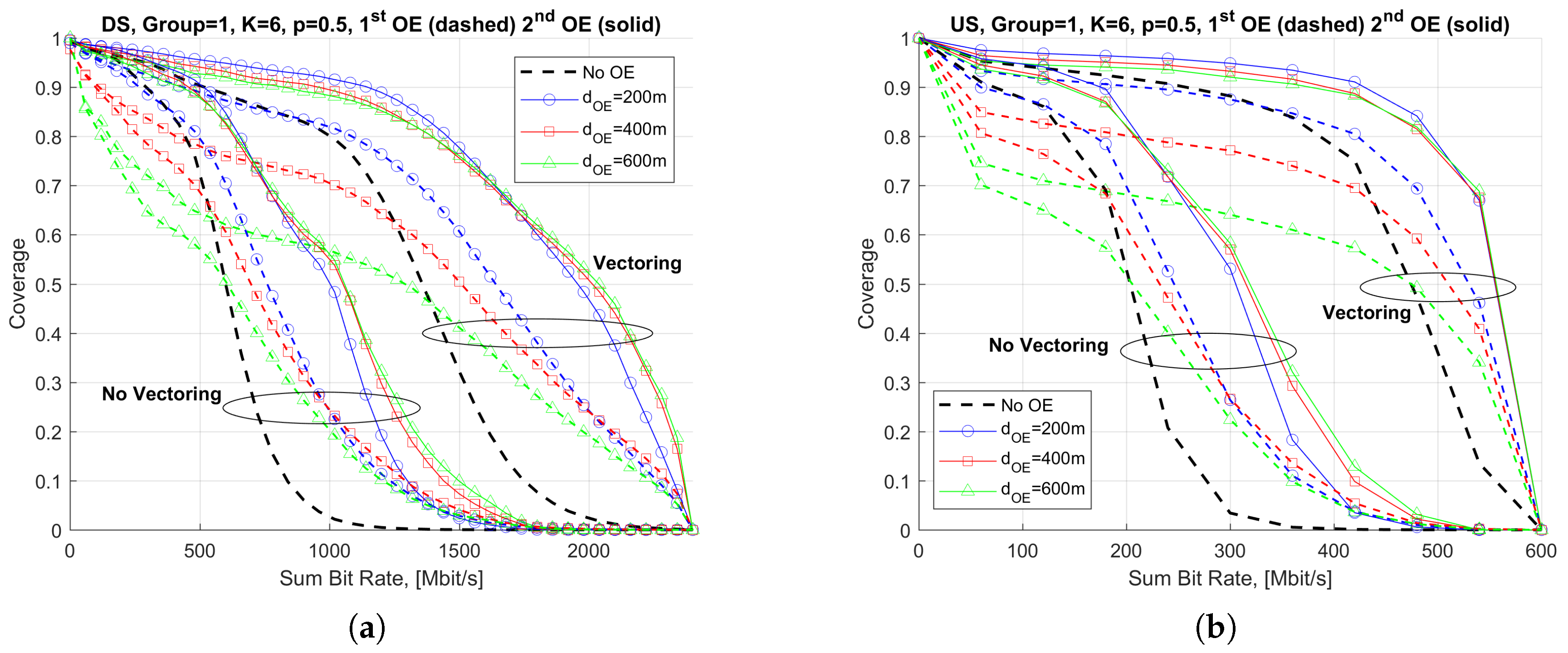
In Figure 5a,b we report the coverage for the target bit rate for group 1 and for DS direction and US direction, respectively. We have considered copper pairs for each radio node and m. In the same figure, vectoring and non-vectoring case have been reported, respectively. Coverage is analyzed for the actual FttC network configuration (indicated as no OE case) and for the extended FttC network considering the two (first and second) evolution strategies illustrated in the previous Section.
As expected, achievable vectoring performance always overcomes non-vectoring. In order to correctly analyze results corresponding to different presented in this and in the following figures it should be noted that coverage statistics for variable have been obtained over the distributors not connected by fiber. The percentage of this distributors is shown in Figure 4 and it decreases with .From results in Figure 5 the first evolution strategy leads to a coverage improvement only for radio nodes close to the new Cabinet at distance from the old one. Results show that adoption of first strategy can be convenient only for small (200 m). In fact, the increase of leads to a reduction of the percentage of distributors connected by copper to the new Cabinet but the proportion of distributors still far from the new Cabinets increases thus leading to a performance reduction. This reduction is indicated by a relatively high percentage of distributors with small bit rates (few tens of Mbit/s) as shown by the green curves in the Figure. This inconvenience can be overcome by considering the second evolution approach where the additional Cabinet is always located in the proximity of the first distributor at distance greater than . This leads to the (almost) invariant behavior of coverage with as shown in the Figure.
It can be observed that, for m, the first evolution approach provides 1 Gbit/s coverage of about 80% for DS and 2 Gbit/s at 25%. Instead, with the second approach coverages of 93% and 48% are obtained for the considered two bit rates, respectively. Similar considerations can be made in the case of US direction as shown in Figure 5b. In particular a target bit rate of 400 Mbit/s can be ensured with a coverage of 82% with the first strategy and about 92% for the second strategy. The two coverage values are not so different. This is due to the most favourable propagation and reduced FEXT conditions in the case of US direction with respect to DS direction due to the lower frequency bands occupied by the US signals.
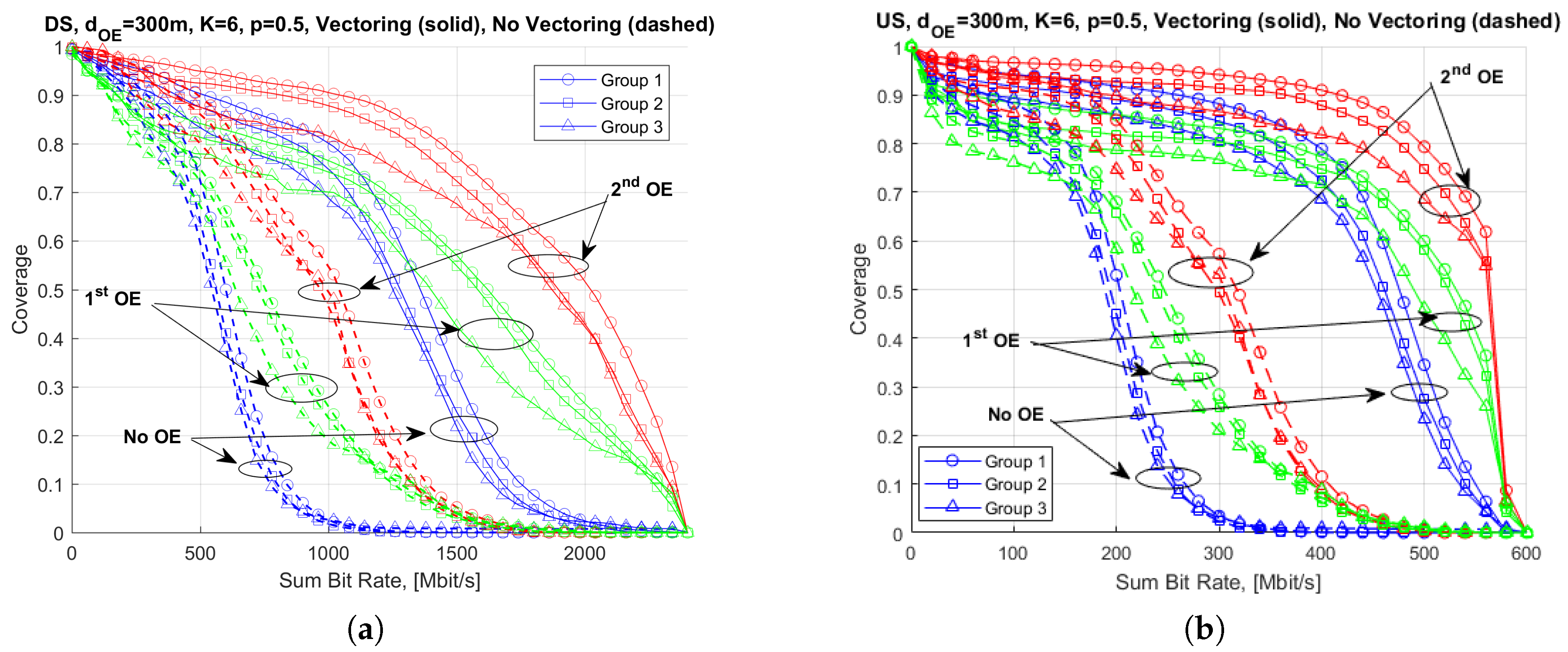
In Figure 6a,b we report the sum bit rate coverage for group 1 and the other two groups for DS direction and US direction, respectively. We have considered copper pairs per node and m. Results in the vectoring case are indicated with solid lines and the results in the non-vectoring case with dashed lines.
Coverages for group 1 and group 2 are close since the CDF of the distance of distributors from the Cabinets are similar as shown in Figure 3. Instead, group 3 performance are worse due to the longer distances of distributors from the respective Cabinets.
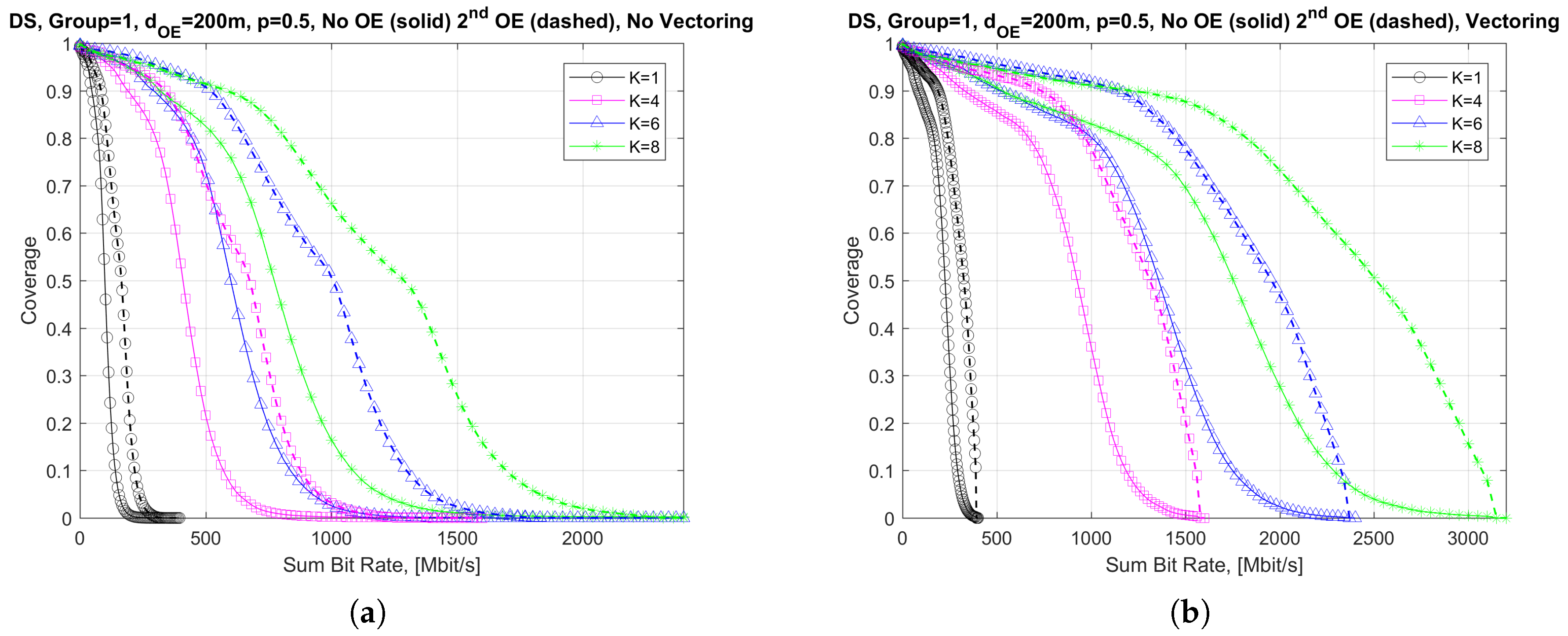
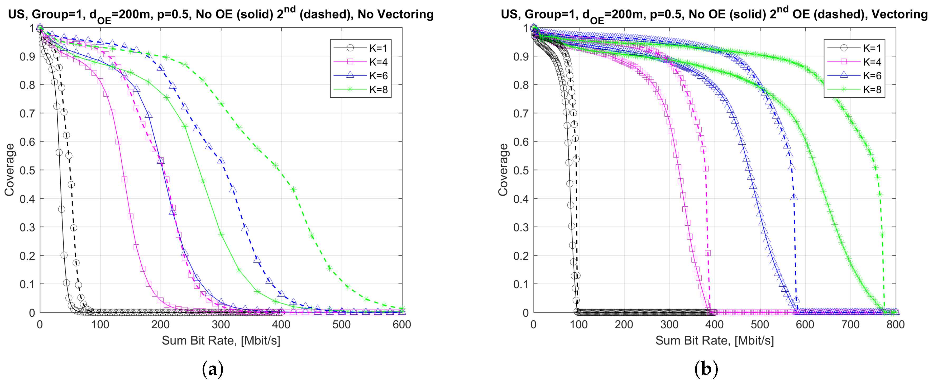
In Figure 7 and Figure 8, we report the group 1 coverage with m and for DS and US, respectively. In these figures, we have varied the number of copper pairs per node K from 1 to 8 and, for simplicity, only the second evolution strategy has been considered.
Coverage increases with the number K of copper pairs. Looking at the curves in Figure 7 and Figure 8 we could assume the sum bit rate is about K times the bit rate obtained for even for distributors at distances from the Cabinet where the FEXT dominates performance (i.e., distances below 400 m). However, this relation would be exact only if copper lines do not interfere each other. Instead, the increase in the number of (active) pairs assigned to each node leads to the increase of FEXT leading to a reduction of performance with respect to the case.
Results in Figure 7 show that coverage of 74% for 2 Gbit/s on DS can be ensured with m and . Concerning US (see Figure 8), up to 600 Mbit/s can be ensured with a coverage of 86% in the same conditions as above.
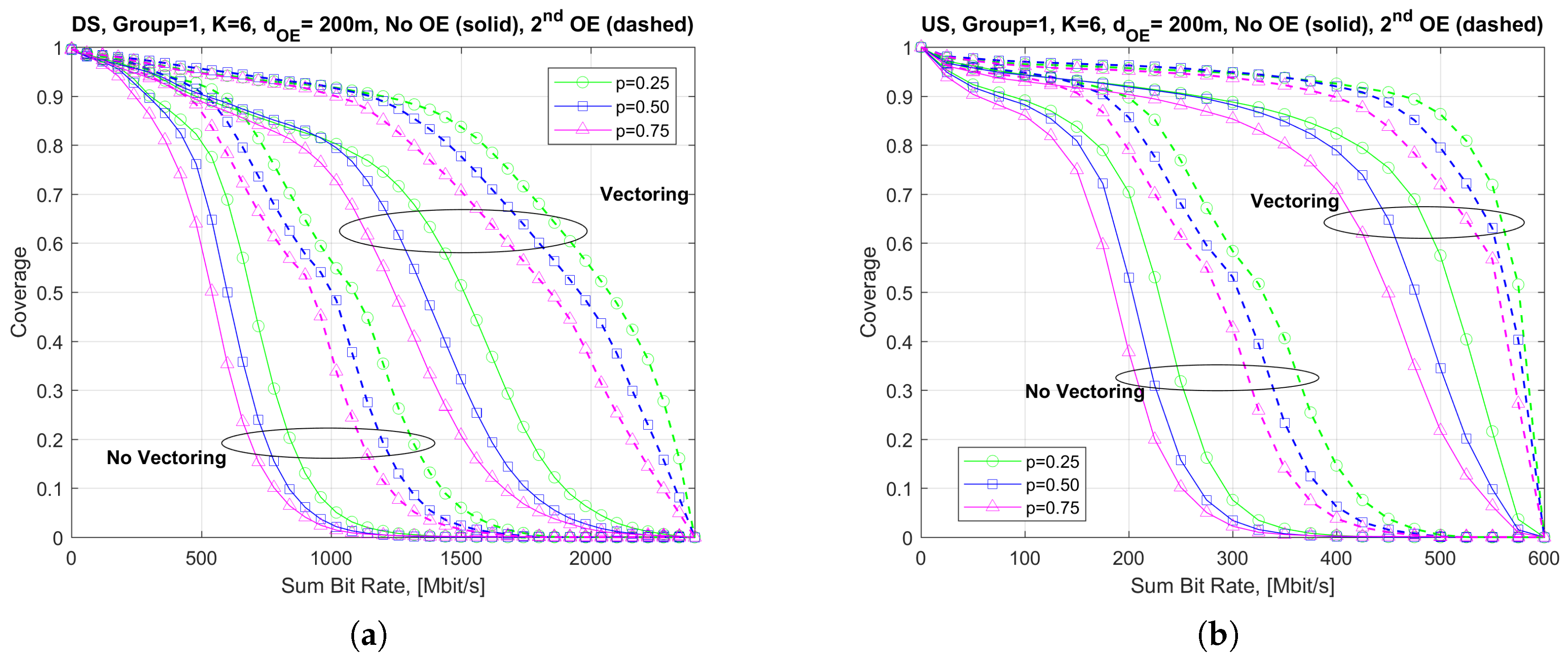
Finally, in Figure 9a,b we study the effects of FEXT variations on the achievable sum bit rate due to the activity of wired subscribers connected to the same cable. Results are presented for the group 1, with , and m and for the case of DS direction and US direction, respectively, and with and without vectoring. Variable activity factors p from 0.25 to 0.75 have been considered for wired subscribers.
The increase of FEXT due to increased activity of wired subscribers leads to a performance reduction causing oscillations in the available fronthauling transport capacity at the radio node. For example, results show that depending on the subscriber activity, the sum bit rate in the DS direction corresponding to the coverage of 80% varies from ±9% with respect to the bit rate obtained for which is about 1.45 Gbit/s for m. Similar considerations apply to the case of US direction. Variability of fronthauling bit rate due to changing FEXT conditions requires the radio node to adapt to the available fronthaul rate as indicated in the previous Section.
5.4. Costs Analysis of Evolved FttC Network with New Added Cabinets
The costs of FttC-based fronthaul using the existing FttC infrastructure only consists in the addition (and installation) of the radio nodes at the distributors. These costs are not considered in the following calculations. Instead, we are interested in the costs of the evolved FttC infrastructure. We assume they can be calculated as the sum of the following three terms: the (overall) costs of digging to lay optical fiber, the cost for new Cabinets and the cost for the equipment to be installed at the distributor connected by fiber, i.e.,
and is the total length of the fiber cables obtained by the sum of the lengths of the optical fiber required to connect the new added Cabinets to the corresponding old Cabinet. The is the unit cost per for digging and installing the optical fiber. Considering conventional digging, the typical value for is 60,000 euro per km [12]. Still, in (20), is the total number of new Cabinets to be added to the existing FttC infrastructure and is the cost per single Cabinet which includes all costs for installation. We have assumed 10,000 euro. Finally, is the number of distributors to be connected by the optical fiber and is the cost of the G.fast or the optical network termination (ONT) to be installed at the distributor for connecting the radio 5G node. We have assumed euro.
The costs of the evolved FttC infrastructure is compared with the cost of a full fiber fronthaul infrastructure where optical fiber is used to connect each distributor to its Cabinet. The formula for evaluating costs in this case is similar to (20) with and equal to the total number of distributors; is the cost of the ONT to be installed at the single distributor and we still assume euro. The is the length of fiber to be deployed and is un-changed.
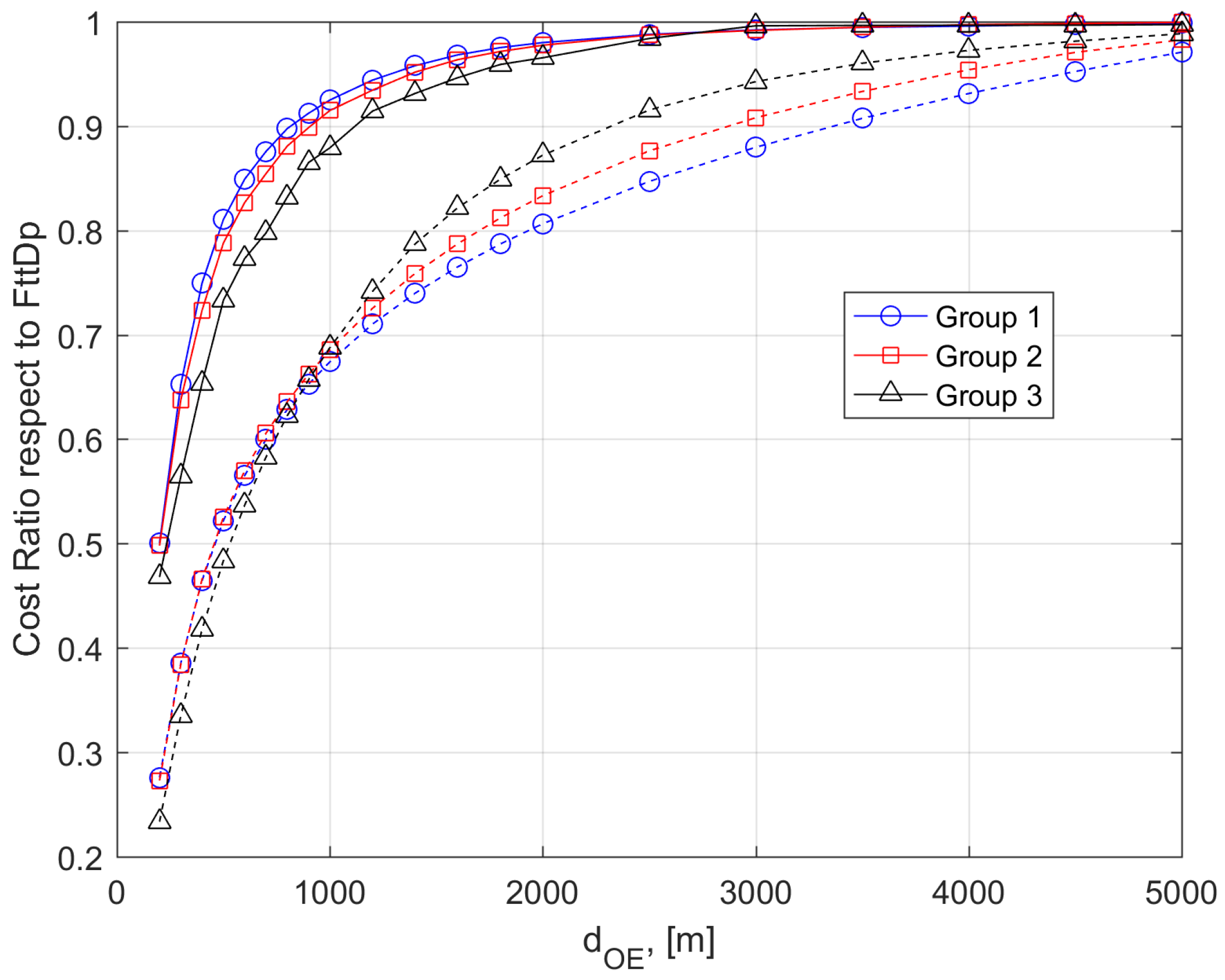
In Figure 10 we plot the cost of the evolved FttC network as compared to the costs of the all-fiber solution as a function of the distance . Results (in percentage) corresponds to the two options in the previous Section.
In both cases, costs tend to increase with since they are dominated by the digging costs for the optical fiber deployment. With the increase of , costs of the evolved FttC network tend to those corresponding to the all-fiber deployment. The first evolution strategy provides lower cost. However, looking for example at coverage results in Figure 5 cost saving is obtained at the expense of reduced coverage performance as compared with results obtained considering the second strategy for the same . In Figure 10 we observe an inversion of costs with . In particular, for small the costs of first strategy are higher for group 1 and group 2 with respect to group 3 and then the situation reverses with the increase of . The inversion of costs still holds for the second strategy even though it occurs for larger and it is not clearly visible in the Figure. The inversion can be explained considering that the distances of distributors in the group 3 are larger than those in the other groups (see Figure 3). Then, in the case of group 3 the possibility of installing a larger number of new Cabinets at longer distances is higher than for group 1 and group 2, thus leading to higher cost for group 3.
6. Effectiveness of FttC-Backhaul
In this section we now briefly discuss on the transport capacity provided by present and the evolved FttC network for future 5G services. We do not focus on specific 5G services but our considerations are confined to the available link capacity for fronthaul as well as on the possibility of using the CPRI or the FAPI interfaces.
From coverage results provided in the previous Section, we can observe that due to the reduced available bandwidth for the case of US direction, in VDSL2 transmissions, it is not possible to use CPRI interface to transport signal samples in the US direction when vectoring is not implemented. Even in the vectoring case, if the number of available pairs (bonded or using phantom) per node is below 8, CPRI cannot be supported. Thus, for transmissions in the US direction on FttC-fronthaul, FAPI and then MAC/PHY splitting seems to be the only viable choice. However, for the DS direction we have evidenced the possibility to support CPRI rates even for relevant percentage of wireless 5G nodes having bit rates about or above 1 Gbit/s in the DS direction. For these nodes the mixed CPRI/FAPI mode discussed in the previous Section could be applied. When considering only the MAC/PHY protocol split option, the achievable fronthaul bit rates for the DS case and the US case give an indication of the gross maximum radio link capacity that can be supported by the single radio node as well as by the radio interface(s) implemented/programmed in the node. To evaluate the net traffic data rate that can be supported on the fronthaul we need to remove the signaling information of the FAPI interface. In general, we observe that vectoring is mandatory for supporting 5G envisaged bit rates. Considering for example results in Figure 5 corresponding to group 1, the target bit rate of 1 Gbit/s in the DS case for each node can be achieved in the 80% of the area. Assuming a uniform distribution of nodes in 1 km2 area and considering the density of the nodes for group 1 in Table 1, the 5G node can provide about 1 Gbit/s on a circular area with radius of about 60 m and this is true for the 80% of radio nodes. In the non-vectoring case this percentage falls down to 3% when 6 copper pairs are assigned to the node. In the non-vectoring case the only way to improve capacity is to increase the number of copper pairs assigned to the radio node. Similar considerations apply to the US case. In this case the sum bit rate corresponding to a coverage of 80% is about 400 Mbit/s. The two considered evolution strategies for the FttC network are helpful to improve the coverage in the (residual) service area still served by FttC. When adopting the second strategy, coverage at 1 Gbit/s can be incremented between 90% and 95% (see Figure 5) depending on the selected which in turns determines the cost for the evolution of the FttC network. In this case, m provides the best performance for 1 Gbit/s at reduced costs with respect to the cases of m and m. Similar considerations apply for cities in group 2 and group 3. For brevity, they are omitted.
7. Conclusions
We have investigated the feasibility of the present FttC fixed access networks to support fronthauling for the forthcoming 5G dense/ultra-dense radio networks as a valuable alternative to optical fiber fronthaul. Our analysis has been restricted to achievable fronthaul capacity only. To this aim, we have assumed that 5G radio nodes can be connected both to the Cabinets and to distributors. Quantitative results have been obtained considering the case of the Italian FttC access network, even though the presented investigation methodology and performance parameters can be easily extended to the analysis of FttC networks in other Countries. We have observe that for large cities, at least, the area density of existing Cabinets and distributors is compatible with that required in a typical 5G ultra-dense deployment for outdoor applications. When vectoring is considered the fronthaul capacity provided to the single access node is about 1 Gbit/s in the DS direction and 400 Mbit/s in the 80% of the service area with six copper pairs (bonded or obtained by phantom) per radio node. Coverage can be increased up to about 95% by adding new Cabinets closer to distributors and, at the same time, connecting part of distributors with the optical fiber. Finally, costs of the proposed extension strategies for the existing FttC networks have been analysed and discussed.
Author Contributions
These authors contributed equally to this work.
Conflicts of Interest
The authors declare no conflict of interest.
References
- Xiang, W.; Zheng, K.; Shen, X.S. 5G Mobile Communications; Springer International Publishing: Basel, Switzerland, 2017. [Google Scholar]
- Ma, Z.; Zhang, Z.Q.; Ding, Z.G.; Fan, P.Z.; Li, H.C. Key techniques for 5G wireless communications: Network architecture, physical layer, and MAC layer perspectives. Sci. China Inf. Sci. 2015, 58, 1–20. [Google Scholar] [CrossRef]
- Wolter, D. Mobile Evolution to 5G: Business Drivers and Technology Enablers for 2020 Networks; CISCO Presentation; CISCO: San Jose, CA, USA, 2015. [Google Scholar]
- Vannithamby, R.; Talwar, S. Towards 5G Applications, Requirements and Candidate Technologies; John Wiley & Sons Ltd.: Hoboken, NJ, USA, 2018. [Google Scholar]
- Gupta, A.; Jha, R.K. A Survey of 5G Network: Architecture and Emerging Technologies. IEEE Access 2015, 3, 1206–1232. [Google Scholar] [CrossRef]
- Wu, G.; Li, Q.C.; Niu, H.; Papathanassiou, A.T. 5G Network Capacity—Key Elements and Technologies. IEEE Veh. Technol. Mag. 2014, 9, 71–78. [Google Scholar]
- Agrawal, R. Mobile Networks Evolution from LTE to 5G: Algorithms and Architecture. Workshop on Information, Decisions, and Networks in Honor of Demos Teneketzis University of Michigan; University of Michigan: Ann Arbor, MI, USA, 2016. [Google Scholar]
- Kamel, M.; Hamouda, W.; Youssef, A. Ultra-Dense Networks: A Survey. IEEE Commun. Surv. Tutor. 2016, 4, 2522–2545. [Google Scholar] [CrossRef]
- Ge, X.; Tu, S.; Mao, G.; Wang, C.X.; Han, T. 5G Ultra-Dense Cellular networks. IEEE Wirel. Commun. 2016, 1, 72–79. [Google Scholar] [CrossRef]
- Schneir, J.R.; Xiong, Y. Cost Analysis of Network Sharing in FTTH/PONs. IEEE Commun. Mag. 2014, 8, 126–134. [Google Scholar] [CrossRef]
- Schindler, J.; Jaillet, J.; Toper, R.; Edwards, J. FTTH Deployment Costs: Expectations vs. Reality. Available online: http://www.ftthcouncil.eu/documents/Reports/2016/WhitePaper-FTTHRolloutCostIndicators.pdf (accessed on 26 October 2017).
- Benedetti, I.; Giuliano, R.; Lodovisi, C.; Mazzenga, F. 5G Wireless Dense Access Network for Automotive Applications: Opportunities and Costs. In Proceedings of the International Conference of Electrical and Electronic Technologies for Automotive, Torino, Italy, 15–16 June 2017; pp. 1–5. [Google Scholar]
- Chang, G.; Cheng, L.; Xu, M.; Guidotti, D. Integrated fiber-wireless access architecture for mobile backhaul and fronthaul in 5G wireless data networks. In Proceedings of the IEEE Avionics, Fiber-Optics and Photonics Technology Conference, Atlanta, GA, USA, 11–13 November 2014. [Google Scholar]
- 5G-Xhaul Project. D2.3 Architecture of Optical/Wireless Backhaul and Fronthaul and Evaluation. Available online: https://bscw.5g-ppp.eu/pub/bscw.cgi/d146395/5G-XHaul_D2_3.pdf (accessed on 26 October 2017).
- Coomans, W.; Moraes, R.B.; Hooghe, K.; Duque, A.; Galaro, J.; Timmers, M.; van Wijngaarden, A.J.; Guenach, M.; Maes, J. XG-Fast: The 5th generation broadband. IEEE Commun. Mag. 2015, 12, 83–88. [Google Scholar] [CrossRef]
- ITU-T G.993.2. Very High Speed Digital Subscriber Line Transceivers 2 (VDSL2); Amendment 2, Recommendation ITU-T G.993.2.; International Telecommunication Union (ITU): Geneva, Switzerland, 2016. [Google Scholar]
- De la Oliva, A.; Hernandez, J.A.; Larrabeiti, D.; Azcorra, A. An overview of the CPRI specification and its application to C-RAN based LTE scenarios. IEEE Commun. Mag. 2016, 2, 152–159. [Google Scholar] [CrossRef]
- Fronthaul Transport for Virtualized Small Cells. Small Cell Forum; Document 169.08.01; University of California: Oakland, CA, USA, 2016; Available online: http://scf.io/en/documents/169_-_Fronthaul_transport_for_virtualized_small_cells.php (accessed on 26 October 2017).
- Dötsch, U.; Doll, M.; Mayer, H.P.; Schaich, F.; Segel, J.; Sehier, P. Quantitative Analysis of Split Base Station Processing and Determination of Advantageous Architectures for LTE. Bell Labs Tech. J. 2013, 1, 105–128. [Google Scholar] [CrossRef]
- Ginis, G.; Cioffi, J.M. Vectored transmission for digital subscriber line systems. IEEE J. Sel. Areas Commun. 2002, 5, 1085–1104. [Google Scholar] [CrossRef]
- Bergel, I.; Leshem, A. The performance of zero forcing DSL systems. IEEE Signal Process. Lett. 2013, 5, 527–530. [Google Scholar] [CrossRef]
- Sorbara, M.; Duvaut, P.; Shmulyian, F.; Singh, S.; Mahadevan, A. Construction of a DSL-MIMO Channel Model for Evaluation of FEXT Cancellation Systems in VDSL2. In Proceedings of the IEEE Sarnoff Symposium, Princeton, NJ, USA, 30 April–2 May 2007; pp. 1–6. [Google Scholar]
- Automatic Terminal Information Service. ATIS Multiple Input Multiple Output Crosstalk Channel Model; ATIS Technical Report NIPP-NAI-2009-014R3; ATIS: Washington, DC, USA, 2009. [Google Scholar]
- Mazzenga, F.; Giuliano, R. Log-normal Approximation for VDSL Performance Evaluation. IEEE Trans. Commun. 2016, 12, 5266–5277. [Google Scholar] [CrossRef]
- Van den Brink, R. G.Fast: Far-End Crosstalk in Twisted Pair Cabling; Measurements and Modelling; ITU-Telecommunication Standardization Sector Temporary Document 11RV-022, ITU-T-SG15; ITU: Geneva, Switzerland, 2011. [Google Scholar]
Figure 1.
Considered 5G dense network architecture with FttC-based fronthaul.
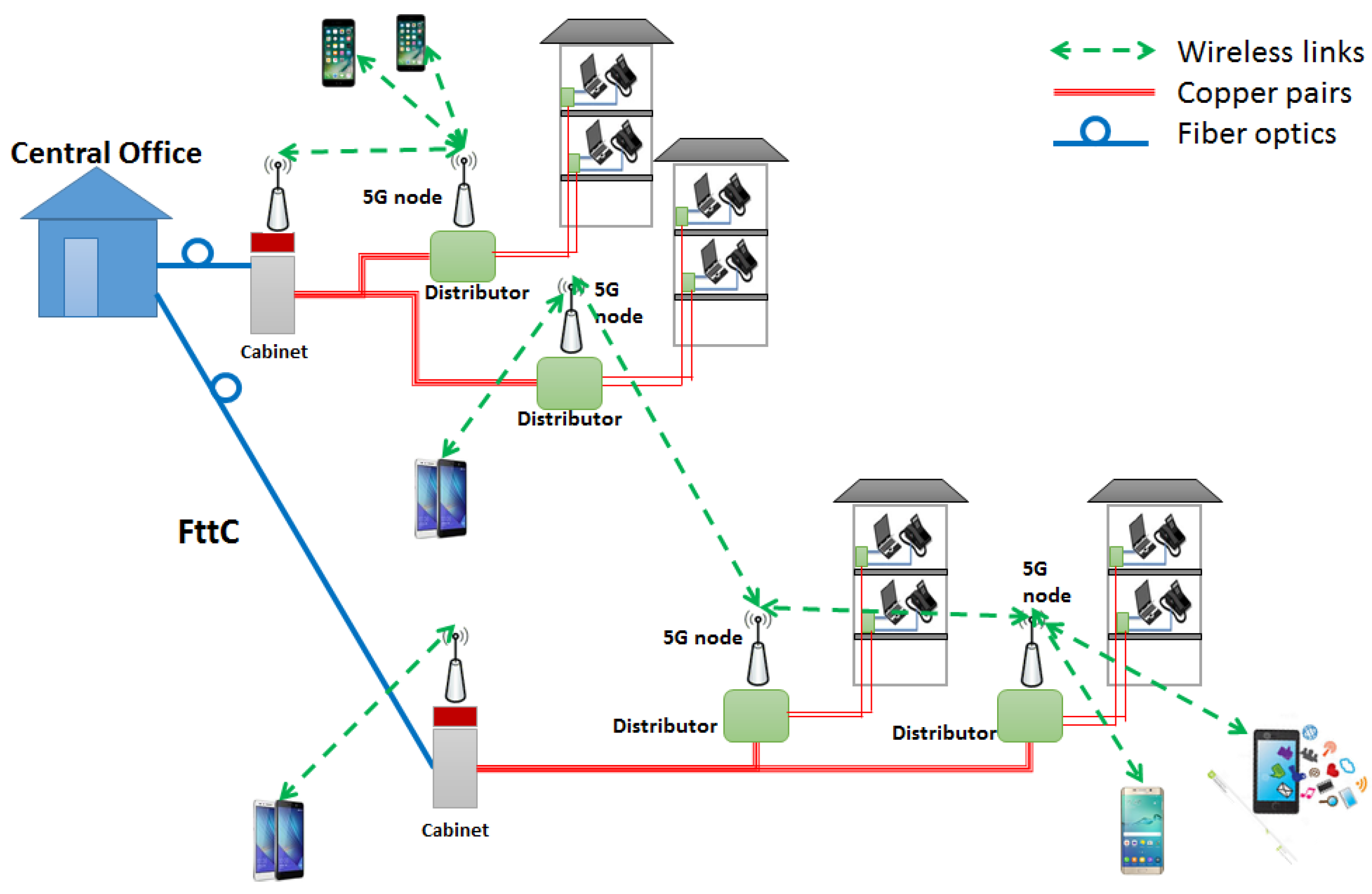
Figure 2.
Protocol stack splitting alternatives: CPRI-based (a); FAPI-based (b).
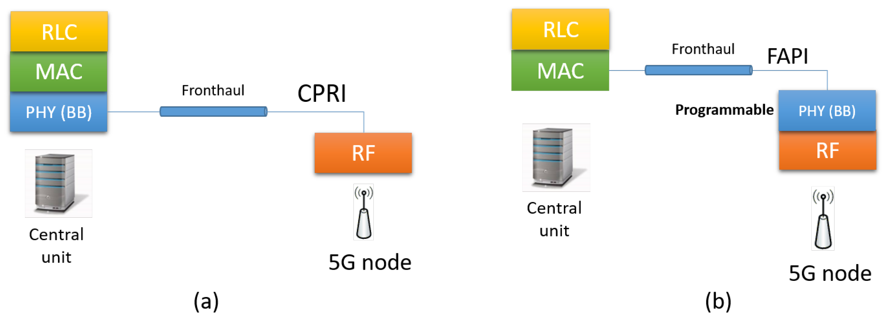
Figure 3.
CDF of the distances of the distributors from the Cabinet in the case of FttC for Italy.
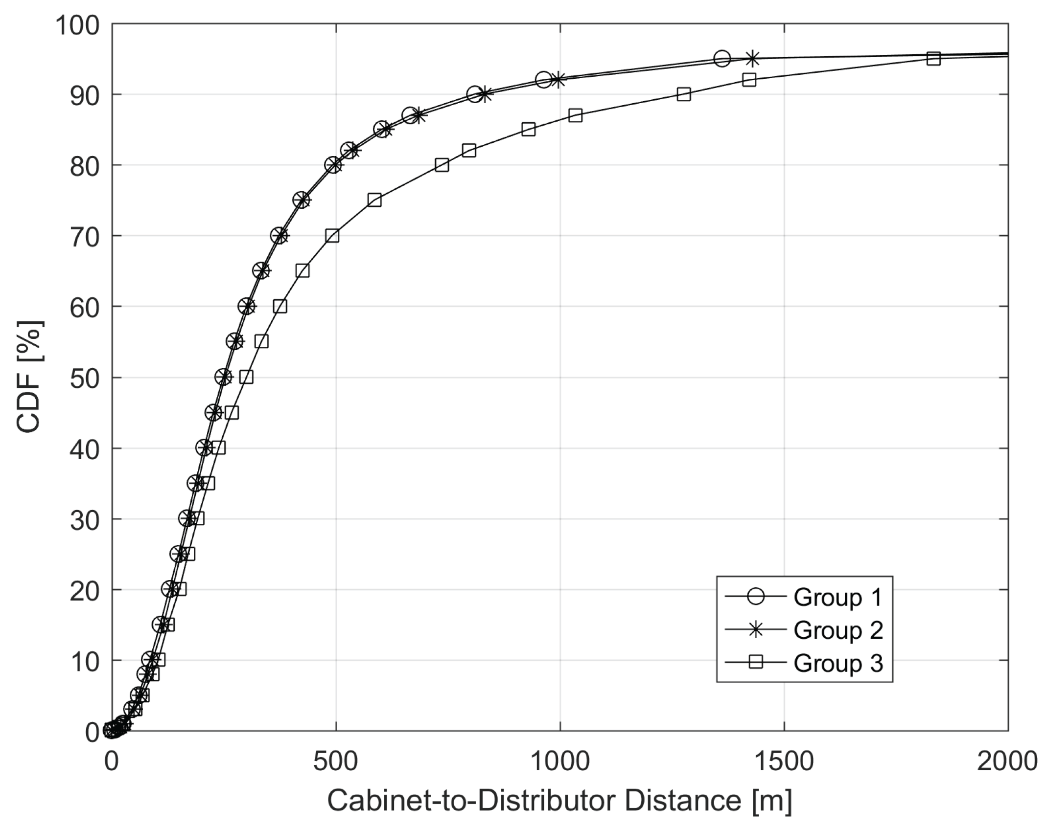
Figure 4.
Percentage of distributors connected by copper to the new added Cabinets as a function of and for the three groups of cities.
Figure 4.
Percentage of distributors connected by copper to the new added Cabinets as a function of and for the three groups of cities.
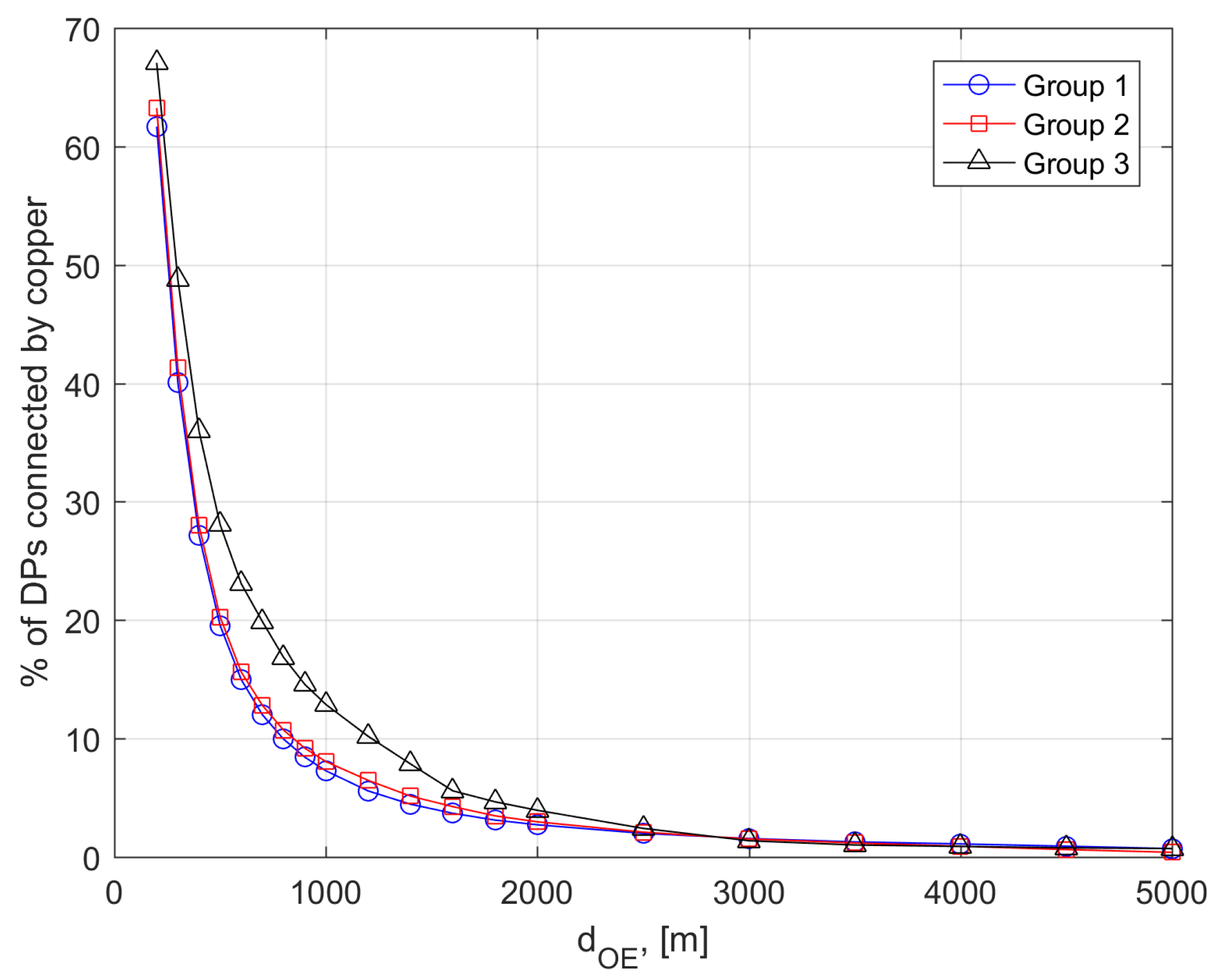
Figure 5.
Sum bit rate coverage for group 1, m—number of pairs assigned to each radio node , user activity factor , vectoring and non-vectoring: DS (a); US (b).
Figure 5.
Sum bit rate coverage for group 1, m—number of pairs assigned to each radio node , user activity factor , vectoring and non-vectoring: DS (a); US (b).

Figure 6.
Sum bit rate coverage for the three groups, m—number of pairs assigned to each radio node , user activity factor , vectoring and non vectoring: DS (a); US (b).
Figure 6.
Sum bit rate coverage for the three groups, m—number of pairs assigned to each radio node , user activity factor , vectoring and non vectoring: DS (a); US (b).

Figure 7.
Sum bit rate coverage for group 1, m—variable of number of pairs per radio node, user activity factor, , DS with non-vectoring (a) and DS with vectoring (b).
Figure 7.
Sum bit rate coverage for group 1, m—variable of number of pairs per radio node, user activity factor, , DS with non-vectoring (a) and DS with vectoring (b).

Figure 8.
Sum bit rate coverage for group 1, m—variable of number of pairs per radio node, user activity factor, , US with non-vectoring (a) and US with vectoring (b).
Figure 8.
Sum bit rate coverage for group 1, m—variable of number of pairs per radio node, user activity factor, , US with non-vectoring (a) and US with vectoring (b).

Figure 9.
Sum bit rate coverage for group 1, m—variable user activity factor p, with and without vectoring: DS (a) and US (b).
Figure 9.
Sum bit rate coverage for group 1, m—variable user activity factor p, with and without vectoring: DS (a) and US (b).

Figure 10.
Cost for the evolved FttC network. Two evolution options: new Cabinets installed at (first option, dashed lines), new Cabinets installed at the distance of the first distributor at distance greater or equal to (second option, solid lines).
Figure 10.
Cost for the evolved FttC network. Two evolution options: new Cabinets installed at (first option, dashed lines), new Cabinets installed at the distance of the first distributor at distance greater or equal to (second option, solid lines).

Table 1.
Average density of distributors for each group.

Table 2.
Updated average density of radio access nodes including the added new Cabinets for each group of cities and for variable .
Table 2.
Updated average density of radio access nodes including the added new Cabinets for each group of cities and for variable .

© 2017 by the authors. Licensee MDPI, Basel, Switzerland. This article is an open access article distributed under the terms and conditions of the Creative Commons Attribution (CC BY) license (http://creativecommons.org/licenses/by/4.0/).
Share and Cite
MDPI and ACS Style
Mazzenga, F.; Giuliano, R.; Vatalaro, F. FttC-Based Fronthaul for 5G Dense/Ultra-Dense Access Network: Performance and Costs in Realistic Scenarios. Future Internet 2017, 9, 71. https://doi.org/10.3390/fi9040071
AMA Style
Mazzenga F, Giuliano R, Vatalaro F. FttC-Based Fronthaul for 5G Dense/Ultra-Dense Access Network: Performance and Costs in Realistic Scenarios. Future Internet. 2017; 9(4):71. https://doi.org/10.3390/fi9040071
Chicago/Turabian StyleMazzenga, Franco, Romeo Giuliano, and Francesco Vatalaro. 2017. "FttC-Based Fronthaul for 5G Dense/Ultra-Dense Access Network: Performance and Costs in Realistic Scenarios" Future Internet 9, no. 4: 71. https://doi.org/10.3390/fi9040071
Note that from the first issue of 2016, this journal uses article numbers instead of page numbers. See further details here.