Article

Research on the Stability Control Strategy of Distributed Electric Vehicles Based on Cooperative Reconfiguration Allocation

1
Key Laboratory of Advanced Manufacturing Technology for Auto Parts, Ministry of Education, Chongqing University of Technology, Chongqing 400054, China
2
College of Mechanical Engineering, Chongqing University of Technology, Chongqing 400054, China
*
Author to whom correspondence should be addressed.
World Electr. Veh. J. 2023, 14(2), 31; https://doi.org/10.3390/wevj14020031
Submission received: 27 December 2022 / Revised: 11 January 2023 / Accepted: 22 January 2023 / Published: 27 January 2023
(This article belongs to the Topic Advanced Electric Vehicle Technology)

Abstract

:
Aiming at the problem of body instability caused by actuator failure in a distributed electric vehicle drive system, a fault-tolerant control strategy of longitudinal and lateral force cooperative reconstruction with active steering control was proposed, and a layered control structure was adopted based on the vehicle model. In the upper controller, the resultant force and torque are calculated according to the vehicle parameter state and MPC algorithm; the lower controller is the cooperative reconfiguration allocation layer, and the minimum tire load rate, longitudinal and lateral force constraints and front wheel angle control are considered. Finally, offline simulation experiments and hardware-in-the-loop experiments are completed to verify the effectiveness and real-time performance of the designed strategy. The results show that the designed strategy can significantly improve the driving stability and safety of the vehicle when the actuator fails.

1. Introduction

In-wheel motors are an emerging technology in recent decades that has led to distributed drive vehicles becoming a research topic for the world’s leading automakers and university research institutions [1], and the electric vehicle market is valuable. However, due to the limitations of its independent drive motor, this is a complex redundant structure and it increases the failure rate of distributed electric vehicles [2]. For this problem, fault-tolerant control originated abroad and was first proposed by Niederlinski in 1971. With the rise of electric vehicles in recent years, many scholars have made great contributions to the study of fault-tolerant control theory [3]. To detect faults in in-wheel motors, Nguyen et al. proposed a Kalman filter algorithm to identify bearing faults in electric in-wheel motors, thereby improving fault detection efficiency [4]. In their studies, some scholars used a Bayesian network, sparse representation, wavelet and other methods to analyze the fault of the wheel hub motor [5,6,7], which can be used for the collaborative development of a fault-tolerant system. In the field of driving state estimation, the scholars Wang et al. and Wang et al. designed a distributed electric vehicle fault diagnosis method. This method was developed to estimate the friction coefficient between the tire and road surface online [8,9]. Zhou et al. combined the Kalman filtering algorithm with a genetic algorithm to reduce the interference of external noise on the estimation results and accurately estimate the longitudinal and transverse speeds, tire force and centroid angle of the vehicle. The simulation verification proves the high precision and high infection robustness of the control algorithm [10]. Chen et al. proposed a vehicle state cascade estimation method to estimate the tire longitudinal force based on an adaptive high-order sliding mode observer combined with an information fusion filtering algorithm, and after the simulation and comparison with the extended Kalman filter algorithm, the superiority of the algorithm was proved [11]. Zhang used the weighted observation fusion Kalman filter algorithm to estimate the longitudinal speed of the vehicle and adopted an improved adaptive Kalman filter algorithm to estimate the vehicle’s yaw angle and yaw angular velocity deviation and observed the state information of other vehicles, estimated the deviation of the lateral velocity and acceleration of the vehicle, and finally obtained the sideslip angle of the vehicle [12]. Aiming to ensure the vehicle’s safety and decrease its instability in the case of an actuator failure, Isa K applied image processing technology to carry out the control simulation of the vehicle driving system, considering the lateral and longitudinal force. This method does not consider the horizontal and vertical complex coupling [13].
Regarding this problem, a comprehensive control strategy for vertical and horizontal motion [14,15,16] and a layered controller [17,18,19] are applied, which obviously solves the coupling and conflict while using multiple electronic control systems and contributes to the vehicle’s running state being more consistent with reality. In this paper, Goodarzi et al. designed a three-layer controller for hybrid vehicles. The first layer tracks the dynamic characteristics of the required vehicle, the second layer determines the optimal tire force and the third layer allocates the power between the engine and the electric motor so that the unstable vehicle is controlled well and its comfort is enhanced [20]. With the popularity of machine learning, a synergistic control algorithm between the lateral and longitudinal coupling is presented by Kumarawadu et al. based on an adaptive neural network model [21]. Certainly, deep learning is also used for controlling the longitudinal and lateral coupling of vehicles. The authors of [22] applied a longitudinal transverse vertical force cooperative fault-tolerant control system of a distributed drive electric vehicle based on longitudinal transverse vertical force. Through comprehensive analysis of actuator redundancy, different fault-tolerant control methods are adopted to comprehensively consider the vehicle state and vertical and horizontal coupling [23]. The MPC algorithm is frequently considered in vertical and horizontal control. In this study, Xia constructed a vehicle longitudinal and lateral coordinated predictive control method under extreme handling conditions, which was based on the MPC algorithm [24]. Subsequently, other scholars Pauca et al. and Wang et al. also utilized the MPC algorithm to calculate the vehicle’s instructions or track control method. Although many scholars at home and abroad have performed a lot of research on actuator failure, the research on the cooperative control of active steering and yaw moment is not enough [25,26].
Aiming at the actuator failure of distributed electric vehicles, in this paper, based on the longitudinal and lateral force cooperative reconstruction distribution, a two-layer fault-tolerant control strategy, which considers the active steering of the front wheels, is proposed. The upper layer employs a model prediction algorithm to follow the longitudinal force, lateral force and the additional yaw moment, which is calculated by the reference state; in the lower layer, its work is to obtain the target tracking torque and front wheel angle via quadratic programming, and the actuator is preliminarily accepted. If a fault occurs, the value will be recalculated by the reconfiguration allocation method to ensure the dynamic performance and stability of the vehicle.

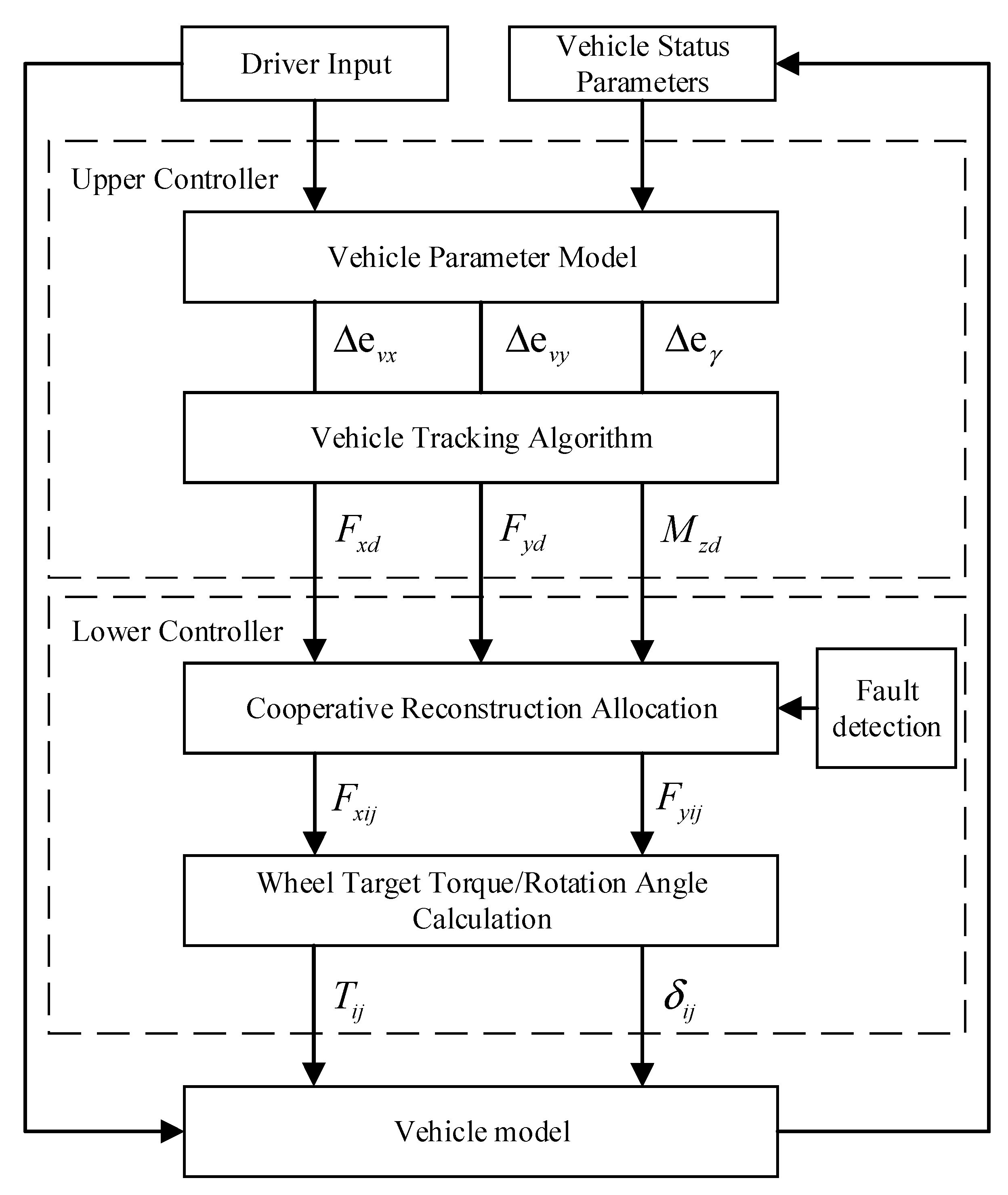
2. Controller Structure Design

Scholars have carried out plentiful research on the fault-tolerant control algorithm of distributed electric vehicles. However, following the expected driving trajectory merely by the additional yaw moment is untoward [27,28]. This paper considers active steering control based on previous studies, which jointly controls the unstable vehicle by active steering and additional yaw moment. Meanwhile, a hierarchical control idea is adopted to construct a fault-tolerant control strategy based on the coordinated reconstruction distribution. The upper layer is the desired trajectory tracking layer. By referring to the vehicle model, the MPC theory is applied to establish a motion-tracking strategy so the vehicle’s resultant force and moment are obtained. The lower layer is the optimized cooperative reconstruction distribution layer. Its function is to recalculate the values, which originate from the upper layer. Figure 1 is the overall workflow of the fault-tolerant control system.

2.1. Vehicle Modeling

2.1.1. Vehicle Dynamics Model
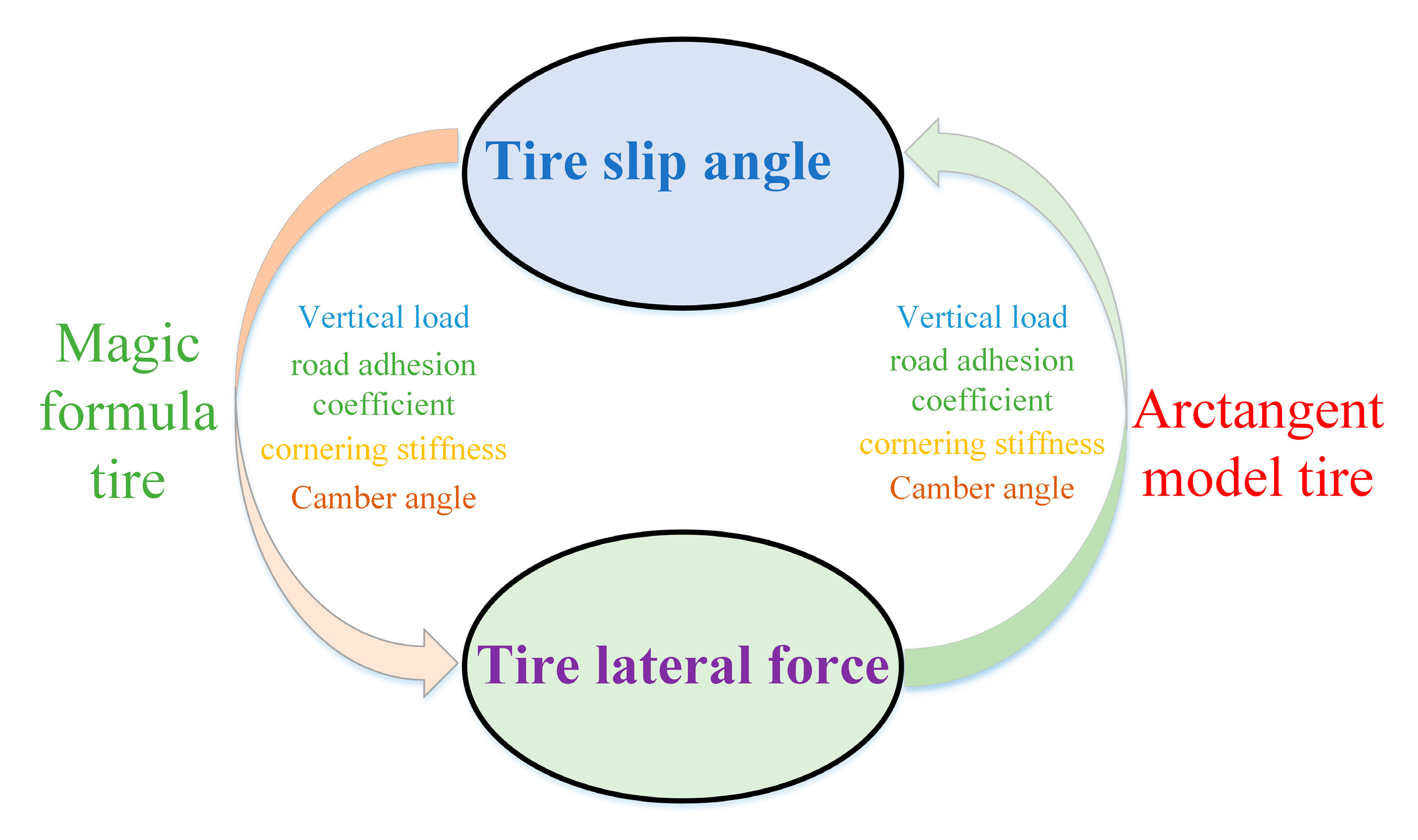
Since only the longitudinal motion, transverse motion and yaw motion of vehicles are considered in this paper, the following vehicle dynamics equation is established according to Newton’s law of motion, as shown in Figure 2.
Longitudinal motion equation of the vehicle:
m ( v · x v y γ ) = ( F x f l + F x f r ) cos δ ( F y f l + F y f r ) sin δ + F x r l + F x r r
Lateral motion equation of the vehicle:
m ( v · y + v x γ ) = ( F x f l + F x f r ) sin δ + ( F y f l + F y f r ) cos δ + F y r l + F y r r
Yaw motion equation of the vehicle:
I z γ · = a ( F x f l + F x f r ) sin δ + 1 2 d ( F x f r F x f l ) cos δ + a ( F y f l + F y f r ) cos δ + 1 2 d ( F y f l F y f r ) sin δ b ( F y r l + F y r r ) 1 2 d ( F x r l F x r r )
where m is the vehicle mass; a and b are the distances from the vehicle’s center of mass to the front and rear axles, respectively; d is the wheel pitch; v x , v y and γ are the longitudinal speed, lateral speed and yaw rate of the vehicle, respectively; F x f l , F x f r , F x r l and F x r r are the longitudinal forces of the left front wheel, right front wheel, left rear wheel and right rear wheel, respectively; F y f l , F y f r , F y r l and F y r r are the lateral force of the left front wheel, right front wheel, left rear wheel and right rear wheel of the vehicle, respectively.

2.1.2. Tire Model

The tire is the carrier of the interaction force between the vehicle and the ground. So, the establishment of the tire model is an essential part of vehicle dynamics research. In this paper, the widely recognized “magic formula” tire model is adopted, which can fit tire test data through the form of a trig function combination, and then the lateral force, longitudinal force and righting moment of the tire can be obtained. The form is expressed as follows:
y ( x ) = D sin { C arctan [ B x E ( B x arctan ( B x ) ) ] } Y ( x ) = y ( x ) + S v x = X + S h
where Y is the dependent variable, such as the tire longitudinal force, lateral force or righting moment; X are the independent variables, such as the tire side slip angle or the longitudinal slip rate; B, C, D and E are the curve stiffness factor, shape factor, peak factor and curvature factor, respectively; S v and S h are the vertical and horizontal offsets of the curves, respectively.
The longitudinal slip rate of each tire is calculated as follows:
s i = { 1 v x i j r ω x i j   ( v x i j < r ω x i j , ω x i j 0 )   Driving   r ω x i j v x i j 1   ( v x i j > r ω x i j , v x i j 0 )     Braking
where v x i j is the center speed of each wheel, r is the rolling radius of the wheel and ω x i j is the angular speed of the wheel ( i j = ( f l , f r , r l , r r ) ).
The side slip angle of each wheel tire is calculated as follows:
{ α f l = arctan v y + a γ v x 0.5 d γ δ f l α f r = arctan v y + a γ v x + 0.5 d γ δ f r α r l = arctan v y b γ v x 0.5 d γ α r r = v y b γ v x + 0.5 d γ
The longitudinal speed of each wheel is calculated as follows:
{ v x f l = ( v x 0.5 d γ ) cos δ + ( v y + a γ ) sin δ v x f r = ( v x + 0.5 d γ ) cos δ + ( v y + a γ ) sin δ v x r l = v x 0.5 d γ v x r r = v x + 0.5 d γ
The dynamic vertical load of each wheel is calculated as follows:
{ F z f l = m ( g b 2 L v · x h 2 L v · y h b d L ) F z f r = m ( g b 2 L v · x h 2 L + v · y h b d L ) F z r l = m ( g b 2 L + v · x h 2 L v · y h b d L ) F z r r = m ( g b 2 L + v · x h 2 L + v · y h b d L )
where L is the wheelbase; h is the height of the center of mass; F z f l , F z f r , F z r l and F z r r are the vertical load of the left front wheel, right front wheel, left rear wheel and right rear wheel, respectively.

2.1.3. Motor Model

Accurate motor modeling can better reflect the dynamic response of the vehicle. Since this paper mainly studies the vehicle stability control after the failure of the distributed electric vehicle drive system, without considering the internal structure of the motor, it is only necessary to establish a motor model that can meet the reaction characteristics. According to the external characteristics of the motor, a constant torque output is generally maintained at a lower speed, and a constant power output is maintained when the rated speed is exceeded, namely, a low-speed constant torque output and a high-speed constant power output. The external characteristic curve of the motor is shown in Figure 3.
The basic equation of torque can be obtained from the motor curve diagram, as follows:
T = { T max   0 n n e 9550 P e n   n e n n max
where T max is the maximum output torque of the motor; n e is the rated motor speed; n max is the maximum speed of the motor; and P e is the rated power of the motor.
Since the instantaneous response speed of the motor is much faster than that of the wheel, in order to accurately simulate the response speed of the motor, this paper adopts the first-order inertia link to simulate the dynamic response process of the motor, and the input-output relationship of the motor torque is as follows:
T o u t = T d 1 1 + τ s
where T d is the input torque of the motor and T o u t is the output torque of the motor. τ is the inertia delay time.

2.2. Upper Controller

2.2.1. Predictive Model

The model predictive control algorithm is advantageous in that no complex models can achieve the same accurate quality control, only the appropriate prediction model can satisfy the constraints of driving conditions [29]. In this paper, the vehicle needs to track the desired trajectory to select the 3-DOF of the vehicle dynamics model-based MPC algorithm, Equation (11), which is given by:
{ x · ( t ) = A c x ( t ) + B c u ( t ) y c ( t ) = C c x ( t )
The parameters are defined as:
x = [ V x V y γ ] ,   y = [ V x V y γ ] ,   A c = [ 0 γ V y γ 0 V x 0 0 0 ] ,
B c = [ 1 / m 0 0 0 1 / m 0 0 0 1 / m ] , C c = [ 1 0 0 0 1 0 0 0 1 ] , u ( t ) = [ Σ F x Σ F y Σ M z ]
where ( Σ F x ,   Σ F y ,   Σ M z ) T is the control variable of the prediction control system and ( V x ,   V y ,   γ ) T are both the control variable and the output variable.
To facilitate subsequent calculations, then discreting Equation (11) and turning it into incremental form leads to Equation (12):
{ Δ x ( k + 1 ) = A m Δ x ( k ) + B m Δ u ( k ) y c ( k ) = C c Δ x ( k ) + y c ( k 1 )
where
Δ x ( k ) = x ( k ) x ( k 1 )
Δ u ( k ) = u ( k ) u ( k 1 )
Based on the principle of the model predictive algorithm, the current state information x ( k ) and y ( k ) are used to predict the state variable within p sampling time, where p = 10. The output sequence is redefined as a new vector matrix form so that the output of the system can be clear the next time, as shown in the following expression, Equation (13):
Y = S x x ( k ) + Φ Δ U
In Equation (13), The specific parameters are
Y = [ y ( k + 1 | k ) y ( k + 2 | k ) y ( k + p | k ) ] p × 1 ,   Δ U = [ Δ u ( k ) Δ u ( k + 1 ) Δ u ( k + m 1 ) ] m × 1 ,   S x = [ C A C A 2 C A p ] p × 1
Φ = [ C B 0 0 C A B C B 0 C A p 1 B C A p 2 B C A p m B ] p × m

2.2.2. Constrained Optimization Solution

The control system mainly enables the vehicle to stably follow the motion of the reference model and restricts the control input of the vehicle from being too large. As a result, the control system cannot solve the problem. In serious cases, the vehicle will deviate from the expected path. Therefore, the objective function is defined as:
J = ( R Y ) T W 1 ( R Y ) + Δ U T W 2 Δ U
where R is the target value for the vehicle’s ideal output. Y is the actual value of the vehicle’s output.
R = [ r ( k ) ,   r ( k + 1 ) r ( k + p 1 ) ] T
W 1 ,   W 2 are a weighted diagonal matrix.
Substituting Equation (13) into Equation (14) leads to:
J = [ R S x x ( k ) ] T W 1 [ R S x x ( k ) ] 2 Δ U T Φ T W 1 [ R S x x ( k ) ] + Δ U T ( Φ T W 1 Φ + W 2 ) Δ U
Equation (15) selects the minimum of the first-order differential. Equation (16) is expressed by:
Δ U = ( Φ T W 1 Φ + W 2 ) 1 Φ T W 1 [ R S x x ( k ) ]
In practice, in order to obtain the best possible system solution, the dynamic response of the vehicle system is also subject to the following constraints:
0 F x d T max R 0 F x d μ m g μ m g F y d μ m g γ min σ γ γ max + σ
where F x d and F y d are the expected longitudinal force and lateral force, respectively; T max is the peak torque motor; γ min and γ max are the minimum yaw rate and maximum yaw rate, respectively; and σ is the relaxation factor.

2.3. Lower Controller

In this paper, the cooperative reconfiguration allocation control algorithm is used to design the lower controller, and its output is divided into normal and fault models. In the normal mode, the desired resultant force and torque are reconstructed and optimally distributed to obtain the target driving torque and front wheel angle. In the fault mode, the target driving torque and front wheel angle under different fault constraints are recalculated.

2.3.1. Optimize the Objective Function

The tire load rate may characterize the driving state during the process of vehicle instability. For example, the smaller the tire force, the more likely a vehicle instability phenomenon will occur. The tire minimum load rate is written as:
min J = i = l r i = f r F x i j 2 + F y i j 2 μ i j 2 F z i j 2
where μ i j is the road adhesion coefficient and F x i j ,   F y i j ,   F z i j are the wheel longitudinal force, lateral force and vertical force, respectively.

2.3.2. Tire Force Constraint

When the desired force and moment are obtained by the upper layer controller to optimize the allocation in the lower layer, each wheel tire force and moment should be balanced. The front wheel angle will exceed its limits as the vehicle is at low speed. It is essential to restrain the longitudinal and lateral tire force accordingly. The restraints are given by:
Σ F x = F x f l + F x f r + F x r l + F x r r Σ F y = F y f l + F y f r + F y r l + F y r r Σ M z = ( F x f r + F x r r ) d 2 ( F x f l + F x r l ) d 2 + ( F y f l + F y f r ) a ( F y r l + F y r r ) b
The range of the tire force is bound by the respective actuator. Considering the constraints of the wheel hub motor capacity is required for each wheel longitudinal force constraint, as follows:
T i j max r i j F x i j T i j max r i j
Similarly, when the vehicle is involved in maximum steering, this will influence the lateral force of each tire. Thus, the restraint is defined as:
F y i j max F y i j F y i j max
When the vehicle is moving, the influence of the attachment ring on the tire shall also be considered. In order to ensure the accuracy of the algorithm and the stability of the vehicle, an external octagon is adopted instead of the attachment circle. The restraint is denoted as:
{ 0.9 μ i j F z i j F x i j 0.9 μ i j F z i j 0.9 μ i j F z i j F y i j 0.9 μ i j F z i j 0.9 2 μ i j F z i j F x i j + F y i j 0.9 2 μ i j F z i j 0.9 2 μ i j F z i j F y i j F x i j 0.9 2 μ i j F z i j

2.3.3. Calculated Wheel Angle

This paper examines the active front steering need for vehicle stability control, to simplify the calculation, with reference to a simplified arctangent tire model, which can characterize the cornering force and tire slip angle [30].
Since the magic formula tire model does not solve the tire slip angle and depends on a large number of fitting data, we used the arctangent model tire to represent the relationship between the lateral force and the tire slip angle. A large number of studies indicated that the tire sideslip characteristics of the two tire models have a high coincidence in the linear region of the tire [31,32,33]. In addition, the tire limit value cannot exceed the adhesion circle in the tire constraint condition. So, the inverse tangent function tire model can meet the accuracy of the tire model in this paper. The logical relationship between the magic formula tire model and the arctangent tire model is shown in Figure 4.
In this arctangent tire model, the relationship between the lateral force and the sideslip angle of the tire is characterized as follows:
F y = f ( α ) = C α G x μ k tan 1 ( k μ α )
where C α is the tire cornering stiffness. The parameters G x = 1 ( F x μ F z ) 2 and k = C α 1 2.9 1 F z are defined.
Then Equation (23) is reversed to obtain the tire slip angle and becomes
α = μ k tan ( k μ 1 C α G x F y )
The sideslip angle of the tire cannot be directly controlled by the vehicle; however, there is a certain conversion relationship between the tire sideslip angle and the wheel angle. The wheel angle can be obtained by Equation (25), as follows:
δ = arctan ( v y + a γ v x 0.5 d γ ) α
where v x and v y are the longitudinal speed and lateral speed, respectively.
Thereby the target front wheel angle is calculated for stability control of the vehicle.

2.3.4. Failure Mode Control Strategy

The wheel hub motor has many sensors and other electronic components. Hence, the distributed electric car is a redundant actuator system; when an actuator fails, the vehicle can maintain stability and safety by distributing the remaining driving force. Therefore, for distributed drive electric vehicles, fault-tolerant control strategies need to be designed to ensure vehicle stability. Through the study of actuator faults, they can be divided into the following six types. For controllable failures, fault-tolerant control can be employed to reconstruct the remaining normal driving wheels to accomplish a new balance and stability of the vehicle. For uncontrollable conditions, the vehicle should choose to brake and stop immediately. The fault-tolerant control strategy of the actuator is shown in Table 1, in which the first three conditions are controllable and the other conditions are uncontrollable.

3. Simulation and Analysis

When the actuator of the drive system fails, in order to verify the effectiveness of the fault-tolerant control algorithm designed in this paper, these aspects include tracking the reference vehicle model and reconstructing the torque distribution and vehicle stability. In this paper, three simulation experiments are designed, and typical front wheel angles are selected for inputting under different working conditions, to compare and verify the effect of improving the stability of the vehicles that adopt a fault-tolerant control strategy. Thus, MATLAB/Simulink is used for building a fault-tolerant control strategy. Meanwhile, the corresponding experimental environment (high adhesion road surface μ = 0.8 , vehicle speed v = 80 km/h) and 7-DOF of the vehicle dynamics model are set. The overall vehicle parameters are shown in Table 2.

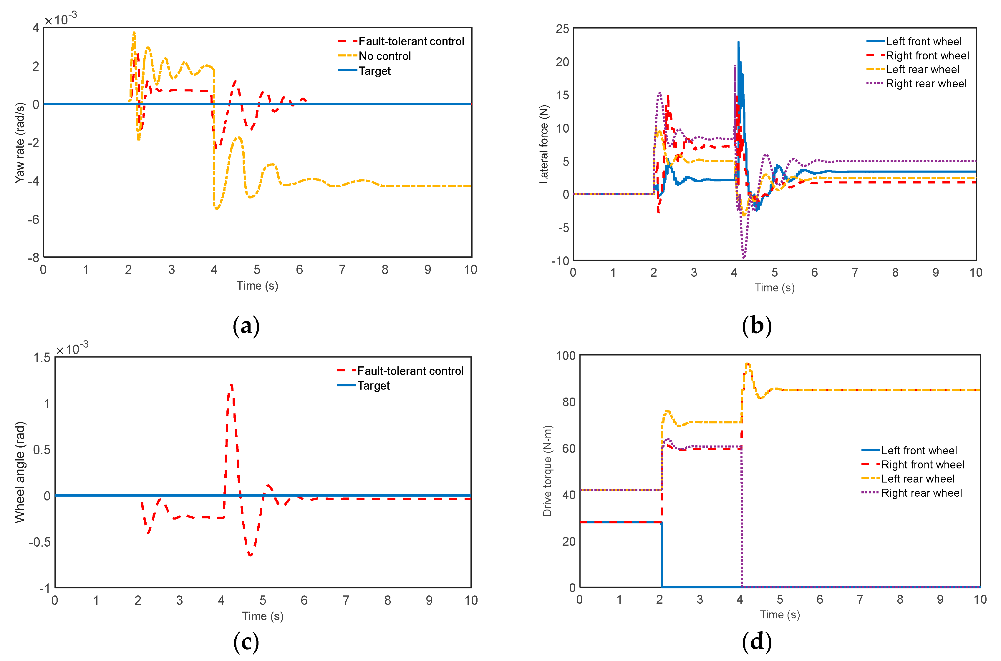
3.1. Double Wheel Failure on a Straight Road

Environment settings: The road adhesion coefficient is 0.8, the speed is 80 km/h and there is a constant zero steering angle. The left front wheel motor fails at 2 s, and the right rear wheel motor fails at 4 s. This purpose primarily verifies whether the fault-tolerant strategy can quickly restore the vehicle to a stable driving state and follow the trajectory simultaneously. The results are shown in Figure 5.
Results analysis: It can be seen from Figure 5a that the vehicle does not swing when traveling straight at the beginning, and the vehicle’s yaw rate is 0. At 2 s and 4 s, the left front wheel and right rear wheel actuators fail successively; however, at 6.2 s, the vehicle with fault-tolerant control keeps up with the expected value and reaches a stable driving state. Within Figure 5b, the vehicle is in a stable state in the first place, the lateral force increases after the vehicle brakes down, and then jitter occurs. The lateral force with the fault-tolerant control is in a reasonable range and does not exceed the limit value of the vehicle instability. Meanwhile, the front wheel angle is amended to maintain the lateral stability of the body. In Figure 5c, we can see that the left front wheel fails at 2 s, and the vehicle generates lateral disturbances to the left and starts to deviate from a straight line. While aiming to maintain a straight-line driving condition, the steering motor can continue to maintain straight-line driving through the right front wheel angle assigned by the upper and lower controllers. Hence, lateral force appears. Similarly, when the right rear wheel fails at 4 s, the vehicle before this movement has reached a new equilibrium, affected by the failure. The vehicle began to display transverse motion, while in the left corner of the front wheels, at 6.2 s, stable driving was resumed. Figure 5d shows the results of the drive torque. Before the failure occurs, the vehicle drive torque is optimally distributed. Additionally, the rear-wheel drive torque is greater than the front-wheel drive torque. At 2 s, the remaining three normal driving motor torques increase and the left rear wheel is greater than the right front and right rear wheels, which generate an additional yaw moment to counteract the vehicle’s lateral offset. At 4 s, the right rear wheel fails and its drive torque instantly becomes 0. The remaining two normal drive motors have increased torque and the torque is equal, to maintain the vehicle drive on a straight road.

3.2. Single-Wheel Fail-in-Step Steering

Environment settings: The rest of the environment settings for this working condition are similar to the above. The only difference is that the driver applies a step of 15° steering wheel angle at 2 s. Meanwhile, the left front wheel actuator fails. Figure 6 shows the results of the simulation.
Results analysis: As can be seen in Figure 6a, the steering angle starts to be applied at 2 s, increasing the yaw rate, and the front left wheel actuator fails and then produces transverse disturbance. The uncontrolled vehicle is unstable. The yaw rate and the expected value generated at the time of 4.2 s show a maximum deviation of 0.025 rad/s and then remain constant. Results analysis: In Figure 6b, the lateral force of the tire is 0. At 2 s, a left front wheel begins to fail, along with transverse disturbance and increasing lateral forces; however, stability soon returned under fault-tolerant control. It can be seen in Figure 6c that the vehicles with fault-tolerant control can follow the vehicle’s expected motion state well, while the vehicles without control are in an unstable state. It is summarized that the designed fault-tolerant control strategy has fine tracking ability and can have a control effect. Figure 6d shows a plot of the driving torque, from which the driving torque is optimally distributed, and the front wheel torque is less than the rear wheel torque. At 2 s, the left front wheel driving torque turns to 0. In this case, the remaining three normal driving motors redistribute the driving torque. The figure shows that the torque increases, and the left rear wheel drive torque is the largest to render the body stable again by the resulting torque. In summary, this explains that the designed fault-tolerant control strategy can significantly improve the vehicle’s power and stability.

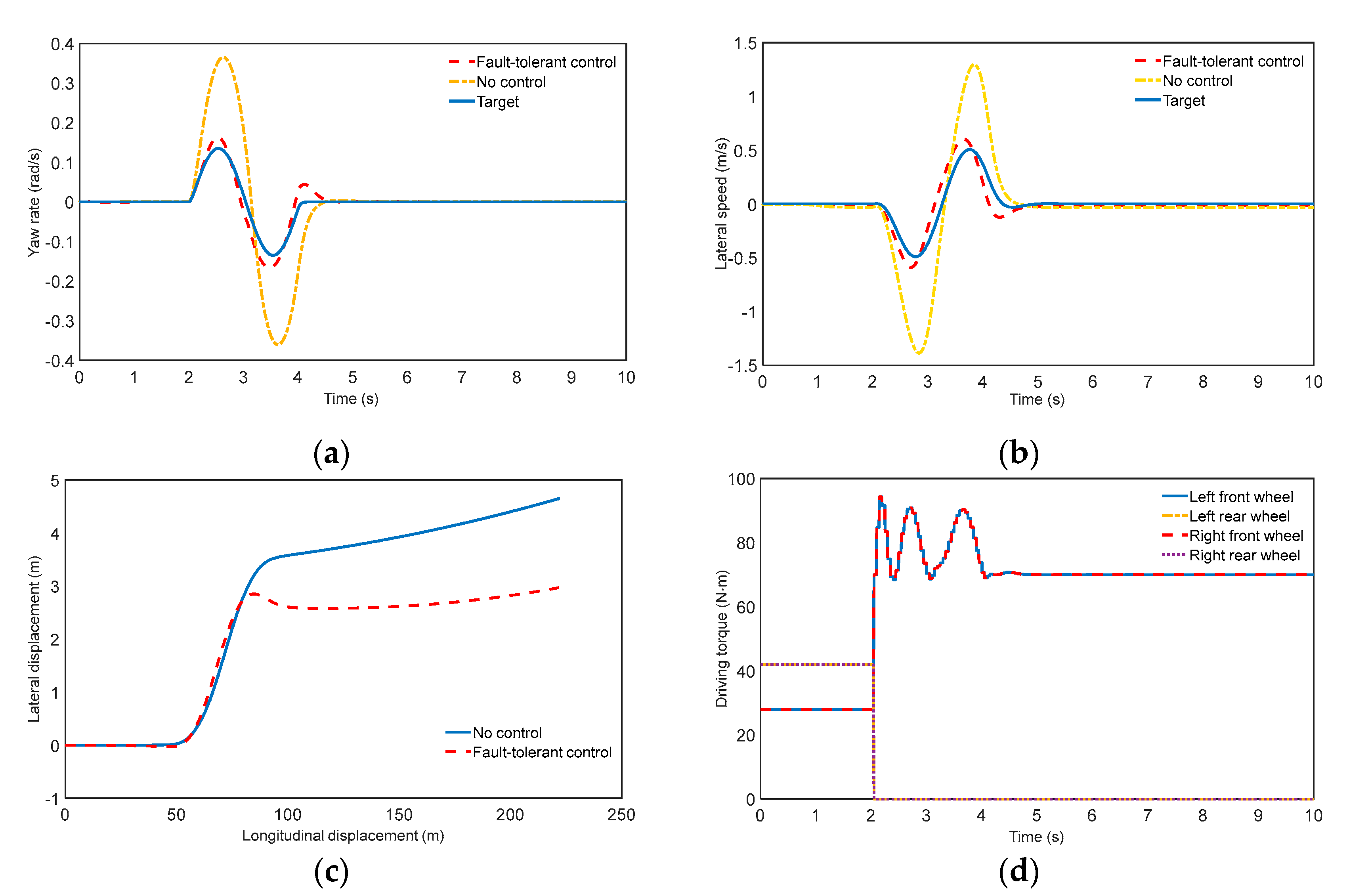
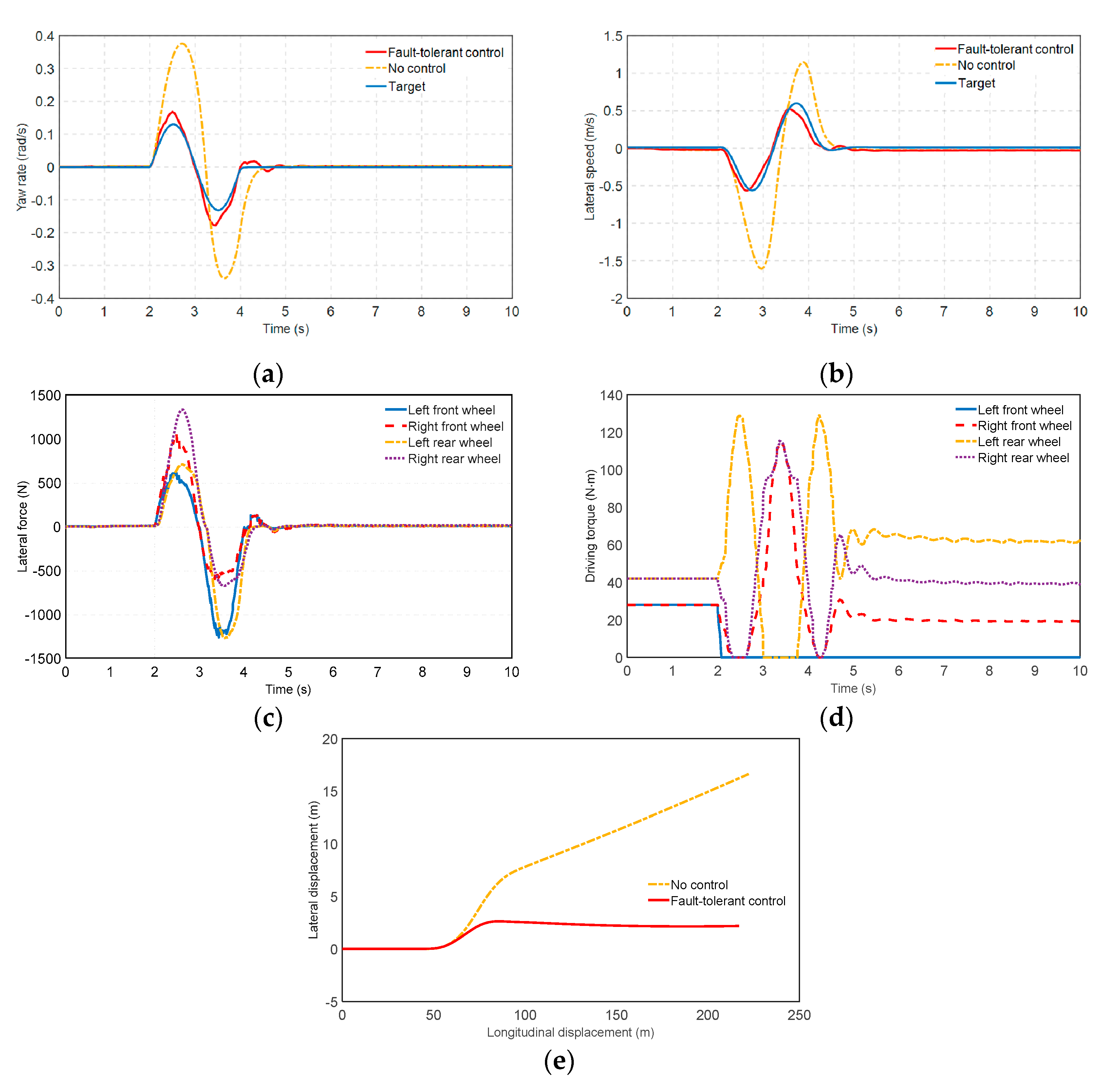
3.3. Double Wheel Failure in Sine Steering

Environment settings: The rest of these environmental conditions are set as above. The only difference is that the left and right rear wheels fail at 2 s, while the driver applies a sinusoidal steering input. Figure 7 reveals the consequences.
Results analysis: It can be observed from Figure 7a,b that the maximum deviation between the yaw rate and its expected value is 0.03 rad/s, and the maximum deviation of the yaw rate is 0.07 m/s. However, the values without fault tolerance are much larger than the values above, the corresponding values of which are 0.25 rad/s and 0.9 m/s. Therefore, the designed fault-tolerant control strategy can effectively follow the driver’s desired driving trajectory. It can be seen in Figure 7c,d that, obviously, the vehicle starts to turn sinusoidally at 2 s, and the left and right rear wheel drive system actuators fail. We can notice that the drive torque of the rear wheel disappears, influencing the vehicle’s stability and decreasing motivation. For vehicles with fault-tolerant control, reconfiguration control is employed to optimize the assignment. It is distinct that the driving torque of the left and right front wheels increases, in the case of retracking the expected movement. When the vehicle steering ends at 4 s, the maximum difference is 1.8 m between those with fault-tolerant control and without fault-tolerant control. The vehicle controlled by fault-tolerant control is in steerable mode, which demonstrates its good movement tracking performance to guarantee the security and stability of the vehicle’s travel.

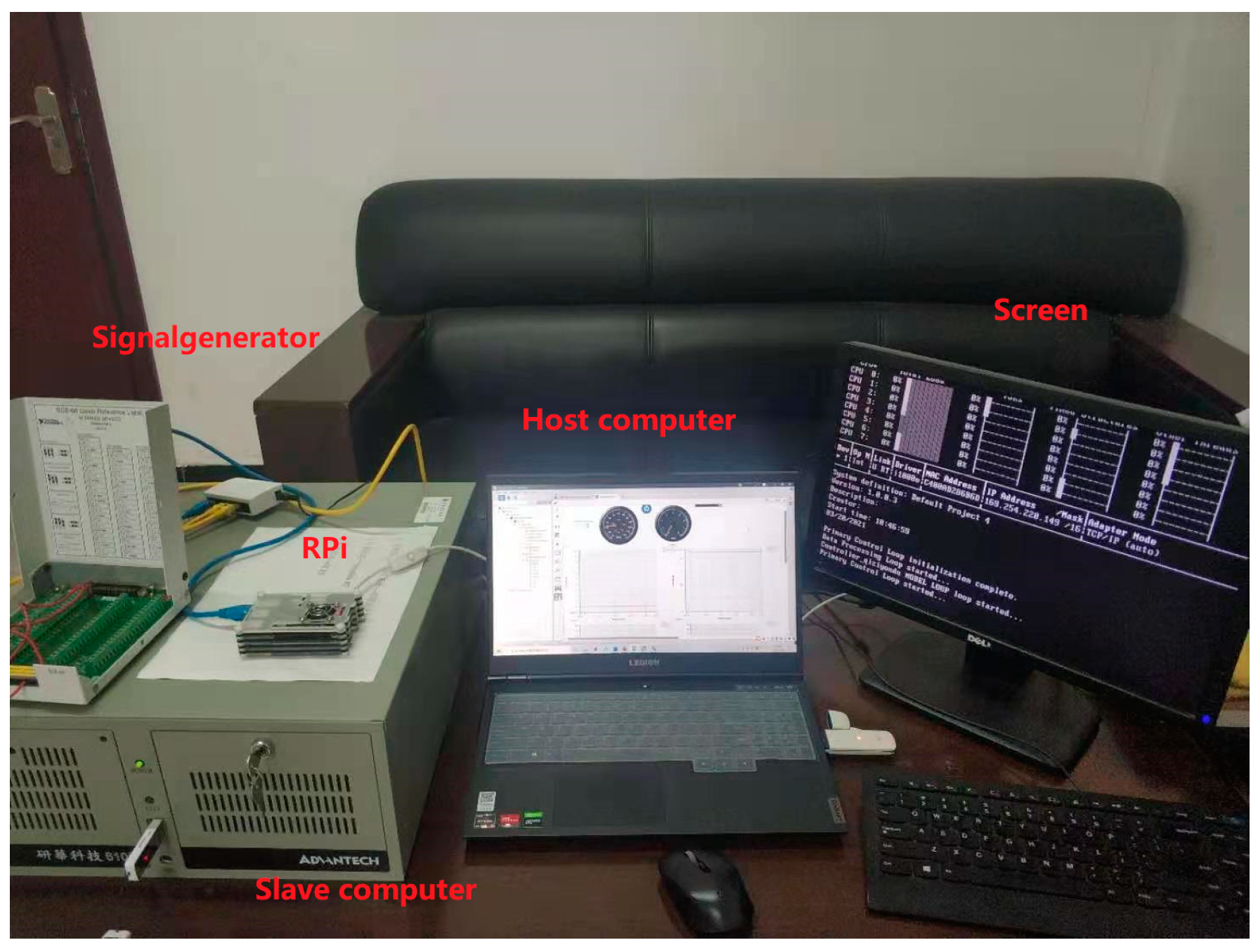
4. HIL Verification and Analysis

The hardware-in-the-loop simulation platform is built using the Ni-PXI real-time system, and the fault-tolerant control algorithm is compiled and downloaded to the raspberry controller. The designed vehicle model needs to be deployed to the real-time system through VeriStrand software, and then the board can be configured and the input and output variables can be mapped. The HIL test platform is shown in Figure 8.
In order to fully verify the real-time performance of the built fault-tolerant control algorithm, the sinusoidal steering input is set to verify the control effect.
Environment settings: The difference between this working condition and the two wheel failures is that the left front-wheel drive system fails at 2 s. Meanwhile, a function signal generator is added that is single-cycle sinusoidal steering. The experimental results are shown in Figure 9.
Results analysis: In Figure 9a,b, the maximum deviation between the yaw rate and its expected value is 0.04 rad/s, and the maximum deviation of the yaw rate is 0.05 m/s. However, the values without fault tolerance are much larger than the values above, the corresponding values of which are 0.27 rad/s and 0.8 m/s. This greatly reduces the yaw stability of the vehicle. Compared with the vehicle without fault-tolerant control, the vehicle with fault-tolerant control can follow the motion of the reference model well at the yaw rate and lateral speed, which improves the vehicle’s yaw stability and lateral stability. An analysis can be seen in Figure 9c; the lateral force and driving torque can well follow the movement of the vehicle and are within the scope of the steady value. Figure 9d,e show the driving torque and motion trajectory curves of the vehicle with fault-tolerant control. In the beginning, the vehicle is following a straight line with no lateral displacement. At 2 s, the vehicle starts to turn sinusoidally and the left front wheel fails. During the turning process, the torque balance of the vehicle is broken, resulting in lateral disturbance and lateral displacement. However, it soon stabilizes under fault-tolerant control. After the fault occurs, the vehicle is reconfigured, and the driving force is optimized to suppress the driving torque of the left front wheel to zero. However, the vehicle is in the right steering condition, the driving torque of the right front wheel and the right rear wheel decreases, and the left rear wheel increases, generating an additional yaw moment and front wheel angle for steering. Between 2 s and 4 s sinusoidal steering of the wheels occurs and the steering is then restored. Compared with fault-tolerant control, the uncontrollable vehicle’s lateral displacement is bigger and has deviated from the desired path severely. An analysis of the figures shows that the vehicle’s drive torque curve trend coincides with one of the steering wheel angles at 5.8 s and maintains stability. These results validate that the built fault-tolerant control strategy has good real-time performance in HIL testing but also prove that it can effectively improve the vehicle’s stability and safety.

5. Conclusions

Aiming at the actuator failure of the distributed electric vehicle, a fault-tolerant control strategy of longitudinal and lateral force cooperative reconfiguration distribution considering active steering control is proposed, and the upper and lower controllers are designed to ensure the stability of the vehicle after the fault occurs.
Three different simulation conditions are set up for the controllable failure conditions. The fault-tolerant control system is built based on MATLAB/Simulink, adopting the driver’s operation as the input. Offline simulation shows that the designed fault-tolerant control algorithm can significantly improve vehicle stability under different fault conditions.
The real-time system based on NI-PXI is built on the HIL test platform, and then the single-wheel fault condition of sinusoidal steering is tested to verify the real-time reliability of the fault-tolerant control algorithm.

Author Contributions

Conceptualization, J.O. and D.Y.; methodology, D.Y.; software, D.Y.; validation, D.Y., D.H. and Y.Z.; formal analysis, E.Y.; investigation, D.H.; resources, E.Y.; data curation, D.Y.; writing—original draft preparation, D.Y.; writing—review and editing, D.Y.; visualization, J.O.; supervision, D.H.; project administration, J.O.; funding acquisition, E.Y. All authors have read and agreed to the published version of the manuscript.

Funding

This research was funded in part by the Special Key Project of Technological Innovation and Application Development in Chongqing (cstc2020jscx-dxwtBX0048) and in part by the Science and Technology Research Project of Chongqing Municipal Education Commission (KJQN201901146).

Data Availability Statement

Not applicable.

Conflicts of Interest

The authors declare no conflict of interest.

References

  1. Hu, Y.; Jiang, F.C.; Chen, R.; Luo, Y.G. Active fault-tolerant control based on MFAC for 4WID EV driving system. Automot. Eng. 2019, 41, 983–989. [Google Scholar]
  2. Tang, Y. Research on Drive System Failure Control for Distributed Drive Electric Vehicles; Harbin Institute of Technology: Harbin, China, 2017. [Google Scholar]
  3. Zhou, D.H.; Ding, X. Theory and applications of fault tolerant control. Acta Autom. Sin. 2000, 26, 788–797. [Google Scholar]
  4. Nguyen, T.-H.; Chen, B.-C.; Yin, D.; Huynh, P.-S. Active fault tolerant torque distribution control of 4 in-wheel motors electric vehicles based on Kalman filter approach. In Proceedings of the 2017 International Conference on System Science and Engineering (ICSSE), Ho Chi Minh City, Vietnam, 21–23 July 2017; pp. 360–364. [Google Scholar] [CrossRef]
  5. Pan, H.M.; Lei, Y.L.; Wang, Z.H. Fault diagnosis of permanent magnets of electric car hub motor based on wavelet analysis. China Mech. Eng. 2016, 27, 1488–1492. [Google Scholar]
  6. Zhou, Z. Research on Fault Diagnosis Method of Hub Motor Bearing Based on Sparse Representation; Jiangsu University: Zhenjiang, China, 2019. [Google Scholar]
  7. Li, Z.X.; Qin, X.; Xue, H.T. In-wheel motor fault diagnosis method based on BN and improved DST. J. Huazhong Univ. Sci. Technol. 2021. [Google Scholar]
  8. Wang, R.; Wang, J. Fault-Tolerant Control for Electric Ground Vehicles With Independently-Actuated In-Wheel Motors. J. Dyn. Syst. Meas. Control. 2012, 134, 021014. [Google Scholar] [CrossRef]
  9. Wang, R.; Wang, J. Actuator-Redundancy-Based Fault Diagnosis for Four-Wheel Independently Actuated Electric Vehicles. IEEE Trans. Intell. Transp. Syst. 2013, 15, 239–249. [Google Scholar] [CrossRef]
  10. Zhou, W.Q.; Qi, X.; Chen, L.; Xu, X. Vehicle state estimation based on the combination of unscented kalman filtering and genetic algorithm. Automot. Eng. 2019, 41, 198–205. [Google Scholar]
  11. Chen, T.; Chen, L.; Cai, Y.F. Cascaded method for running state estimation of four-wheel independent drive electric vehicles. J. Cent. South Univ. 2019, 50, 241–249. [Google Scholar]
  12. Zhang, L. Research on State Estimation and Torque Vectoring Control of Distributed Drive Electric Vehicles; Jilin University: Changchun, China, 2019. [Google Scholar]
  13. Isa, K. Experimental Studies on Dynamics Performance of Lateral and Longitudinal Control for Autonomous Vehicle Using Image Processing. In Proceedings of the IEEE International Conference on Computer & Information Technology Workshops, Sydney, Australia, 8–11 July 2008; pp. 411–416. [Google Scholar] [CrossRef] [Green Version]
  14. Jalali, K.; Uchida, T.; McPhee, J.; Lambert, S. Development of an Integrated Control Strategy Consisting of an Advanced Torque Vectoring Controller and a Genetic Fuzzy Active Steering Controller. SAE Int. J. Passeng. Cars Electron. Electr. Syst. 2013, 6, 222–240. [Google Scholar] [CrossRef] [Green Version]
  15. Katriniok, A.; Maschuw, J.P.; Christen, F.; Eckstein, L.; Abel, D. Optimal vehicle dynamics control for combined longitudinal and lateral autonomous vehicle guidance. In Proceedings of the European Control Conference, Zurich, Switzerland, 17–19 July 2013. [Google Scholar] [CrossRef]
  16. Xie, B.Y. Vehicle Cooperative Control Based on Information Exchange and Motion Coupling; Tsinghua University: Beijing, China, 2014. [Google Scholar]
  17. Dai, Y.F. Integrated Longitudinal and Lateral Motion Control of Distributed Electric Vehicles; Tsinghua University: Beijing, China, 2013. [Google Scholar]
  18. Jiao, G.K. Study on Longitudinal and Lateral Force Coordinated Control of Four Wheel Independent Driving/Steering Electric Vehicle; Chongqing University: Chongqing, China, 2018. [Google Scholar]
  19. Amato, G.; Marino, R. Fault-Tolerant Distributed and Switchable PI Slip Control Architecture in Four In-Wheel Motor Drive Electric Vehicles. In Proceedings of the Mediterranean Conference on Control and Automation (MED), Saint-Raphael, France, 16–18 September 2020; pp. 7–12. [Google Scholar] [CrossRef]
  20. Goodarzi, A.; Mohammadi, M. Stability enhancement and fuel economy of the 4-wheel-drive hybrid electric vehicles by optimal tyre force distribution. Veh. Syst. Dyn. 2013, 52, 539–561. [Google Scholar] [CrossRef]
  21. Kumarawadu, S.; Lee, T.T. Neuroadaptive Combined Lateral and Longitudinal Control of Highway Vehicles Using RBF Networks. IEEE Trans. Intell. Transp. Syst. 2006, 7, 500–512. [Google Scholar] [CrossRef]
  22. Devineau, G.; Polack, P.; Altche, F.; Moutarde, F. Coupled Longitudinal and Lateral Control of a Vehicle using Deep Learning. In Proceedings of the Conference on Intelligent Transportation Systems, Maui, HI, USA, 4–7 November 2018; pp. 642–649. [Google Scholar] [CrossRef] [Green Version]
  23. Luo, Y.; Cao, K.; Li, K. Coordinated Control of Longitudinal/Lateral/Vertical Tire Forces for Distributed Electric Vehicles; Tsinghua University: Beijing, China, 2014. [Google Scholar] [CrossRef]
  24. Xia, Z.K. Research on Fault-Tolerant Control Method of Yaw Stability of Distributed Electric Vehicle; Chongqing University of Technology: Chongiqng, China, 2019. [Google Scholar]
  25. Pauca, O.; Caruntu, C.F.; Lazar, C. Predictive control for the lateral and longitudinal dynamics in automated vehicles. In Proceedings of the 2019 23rd International Conference on System Theory, Control and Computing (ICSTCC), Sinaia, Romania, 8–11 October 2019; pp. 797–802. [Google Scholar]
  26. Wang, R.C.; Wei, Z.D.; Ye, Q. A research on visual preview longitudinal and lateral cooperative control of intelligent vehicle. Automot. Eng. 2019, 41, 763–770. [Google Scholar]
  27. Rajamani, R. Vehicle Dynamics and Control; Springer Science & Business Media: New York, NY, USA, 2011. [Google Scholar]
  28. Dai, Y.F.; Luo, Y.G.; Li, K.Q. Dynamic coordinated control for a full hybrid electric vehicle with single motor. Automot. Eng. 2011, 33, 1007–1012. [Google Scholar]
  29. Liu, J.; Jayakumar, P.; Overholt, J.L.; Stein, J.L.; Ersal, T. The Role of Model Fidelity in Model Predictive Control Based Hazard Avoidance in Unmanned Ground Vehicles Using LIDAR Sensors. In Proceedings of the Dynamic Systems and Control Conference, Palo Alto, CA, USA, 21–23 October 2013. [Google Scholar] [CrossRef] [Green Version]
  30. Shin-Ichiro, S.; Hideo, S.; Yoichi, H. Dynamic driving/braking force distribution in electric vehicle with independently driven four heels. IEEE Trans. Ind. Appl. 2000, 138, 79–89. [Google Scholar]
  31. Kranz, T.; Hahn, S.; Zindler, K. Nonlinear Lateral Vehicle Control in Combined Emergency Steering and Braking Maneuvers. In 2016 IEEE Intelligent Vehicles Symposium (IV); IEEE: Manhattan, NY, USA, 2016; pp. 603–610. [Google Scholar]
  32. Wang, H.; Han, J.; Zhang, H. Lateral Stability Analysis of 4WID Electric Vehicle Based on Sliding Mode Control and Optimal Distribution Torque Strategy. Actuators 2022, 11, 244. [Google Scholar] [CrossRef]
  33. Zhang, B.; Lu, S. Fault-tolerant control for four-wheel independent actuated electric vehicle using feedback linearization and cooperative game theory. Control Eng. Pract. 2020, 101, 104510. [Google Scholar] [CrossRef]
Figure 1. Overall workflow of the fault-tolerant control system.
Wevj 14 00031 g001
Figure 2. Vehicle dynamics model.
Wevj 14 00031 g002
Figure 3. Motor external characteristic curve.
Wevj 14 00031 g003
Figure 4. Tire force and slip angle conversion relationship.
Wevj 14 00031 g004
Figure 5. Results of two failed wheels on a straight road: (a) Yaw rate; (b) Lateral force; (c) Wheel angle; (d) Drive torque.
Wevj 14 00031 g005
Figure 6. Results of the single-wheel failure in the angular step steering: (a) Yaw rate; (b) Lateral force; (c) Sideslip angle; (d) Drive torque.
Wevj 14 00031 g006
Figure 7. Results of the two failed wheels in sinusoidal steering: (a) Yaw rate; (b) Lateral speed; (c) Motion trajectory; (d) Drive torque.
Wevj 14 00031 g007
Figure 8. HIL test platform.
Wevj 14 00031 g008
Figure 9. Results of the single failed wheel in sinusoidal steering: (a) Yaw rate; (b) Lateral speed; (c) Lateral force; (d) Drive torque; (e) Motion trajectory.
Wevj 14 00031 g009
Table 1. Failure mode control policies.
Failure ModeFailure Constraints (Example)Controllable or Not
A single drive motor failure F x f l = 0 Controllable
Two diagonal drive motors failure F x f l = 0 , F x r r = 0 Controllable
Two coaxial drive motors failure F x r l = 0 , F x r r = 0 Controllable
Two ipsilateral drive motors failure F x f l = 0 , F x r l = 0 Uncontrollable
Three drive motors failure F x f l = 0 , F x f r = 0 , F x r l = 0 Uncontrollable
Four drive motors failure F x f l = 0 , F x f r = 0 , F x r l = 0 , F x r r = 0 Uncontrollable
Table 2. Vehicle model parameters.
Vehicle ParametersValues
Vehicle mass ( m / kg ) 870
Distance from front axle to center of mass ( a / m ) 1.013
Distance from rear axle to center of mass ( b / m ) 0.702
Centroid height ( h / m ) 0.51
Moment of inertia ( I z / ( kg m 2 ) ) 617
Wheel pitch ( d / m ) 1.3
Wheel radius ( r / m ) 0.302
Peak power ( P max / W ) 6900
Rated power ( P e / W ) 4700
Maximum speed ( n max / ( r min 1 ) ) 1055
Rated speed ( n e / ( r min 1 ) ) 440
Peak torque ( T max / ( N m ) ) 150
Time constant ( τ / s ) 0.01
Road adhesion coefficient ( μ ) 0.8
Disclaimer/Publisher’s Note: The statements, opinions and data contained in all publications are solely those of the individual author(s) and contributor(s) and not of MDPI and/or the editor(s). MDPI and/or the editor(s) disclaim responsibility for any injury to people or property resulting from any ideas, methods, instructions or products referred to in the content.

