

Decoupling Control of Yaw Stability of Distributed Drive Electric Vehicles
1
Xinjiang Institute of Technology, School of Mechanical and Electrical Engineering, Akesu 843000, China
2
College of Mechanical and Electrical Engineering, Shihezi University, Shihezi 832000, China
*
Author to whom correspondence should be addressed.
World Electr. Veh. J. 2024, 15(2), 65; https://doi.org/10.3390/wevj15020065
Submission received: 5 January 2024
/
Revised: 31 January 2024
/
Accepted: 5 February 2024
/
Published: 14 February 2024
(This article belongs to the Special Issue Vehicle System Dynamics and Intelligent Control for Electric Vehicles)
Abstract
:Most of the research on driving stability control of distributed drive electric vehicles is based on a yaw motion design controller. The designed controller can improve the lateral stability of the vehicle well but rarely mentions its changes to the roll and pitch motion of the body, and the uneven distribution of the driving force will also cause instability in the vehicle speed, resulting in wheel transition slip, wheel sideslip, and vehicle stability loss. In order to improve the spatial stability of distributed-driven electric vehicles and resolve the control instability caused by their motion coupling, a decoupled control strategy of yaw, roll, and pitch motion based on multi-objective constraints was proposed. The strategy adopts hierarchical control logic. At the upper level, a yaw motion controller based on robust model predictive control, a roll motion controller, and a pitch motion controller based on feedback optimal control are designed. In the lower level, through the motion coupling analysis of the vehicle yaw control process, based on the coupling analysis, the vehicle yaw, roll, and pitch decoupling controller based on multi-objective constraints is designed. Finally, the effectiveness of the decoupling controller is verified.
1. Introduction
With energy conservation and emission reduction becoming the focus of public concern, electric vehicles have been receiving more attention in recent years [1,2]. As a new type of drive for electric vehicles, distributed drive has various advantages, such as simple structure and easy control, which is one of the important development directions of new energy vehicles in the future [3,4,5,6,7,8,9,10,11,12]. Research on driving stability control for distributed drive electric vehicles is becoming more mature as well as diverse. For example, in order to solve the problem of wireless wheel motors where the supplied secondary side voltage changes due to misalignment of the wheel and the body, a method of maintaining the secondary voltage using a hysteresis comparator is proposed for efficiently driving the wireless wheel [13]. Luque P et al. proposed an iterative algorithm for determining the optimal chassis design for an electric vehicle given a path and reference time. The proposed algorithm balances the capacity of the battery pack with the dynamic characteristics of the chassis and seeks to optimize the trade-off between vehicle mass, energy consumption, and travel time [14]. Liang Y et al. proposed a scalable vehicle state estimation concept that fuses conventional vehicle sensors with environmental sensors using the Error State Extended Kalman Filter (ESEKF) to ensure the accuracy and robustness of redundant sensor data under conventional and dynamic driving conditions [15]. Shahian Jahromi B et al. used encoder–decoder-based Fully Convolutional Neural Networks (FCNx) and traditional Extended Kalman Filter (EKF) nonlinear state estimation methods. Camera, LiDAR, and radar sensor configurations best suited to each fusion method are used to provide a fusion system solution that is cost-effective, lightweight, modular, and robust (in the event of sensor failure) [16]. D. Tian et al. proposed a parameter estimation method based on multidimensional information fusion to achieve real-time accurate acquisition of reference speed, mass, and road gradient [17]. Yang S et al. proposed a method to robustly estimate vehicle attitude by fusing data collected by 4D radar and camera. The proposed method shows excellent performance and enhanced robustness in visually challenging scenarios such as foggy environments [18]. Farag W et al. used a traceless Kalman filter to fuse LiDAR and radar measurements in order to accurately provide driverless vehicles with position and velocity information about objects moving on the surrounding road [19]. Gao et al. proposed a target classification method based on convolutional neural networks and image up-sampling theory to obtain informative feature representations in self-driving car environments using integrated visual and optical detection and ranging data. As a result, they developed a trajectory prediction model combining physical- and maneuver-based models to solve the nonlinear estimation and prediction problem, and this interactive multi-model trajectory prediction method can make more accurate predictions than a single model [20]. Desjardins et al. used approximation and gradient descent learning algorithms to implement queue control for vehicles and optimize their consistency [21]. Chong L et al. used data such as the driver’s own characteristics, relative motion relationships, and environmental factors as system inputs. They developed a driver model based on a fuzzy neural network, which simulated the driving characteristics of a vehicle during longitudinal automatic control [22]. Aiming at the problem that it is difficult to obtain the optimal driving strategy for automated vehicle driving in complex environments and variable task conditions, Lin J et al. proposed an end-to-end automated driving strategy learning method based on deep reinforcement learning, which effectively improves the efficiency of automated driving strategy learning and controlling virtual vehicles and provides reliable theoretical and technical support for real vehicles in the decision-making of automated driving [23]. Kumar GA et al. proposed a method to estimate the distance (depth) between a self-driving car and other vehicles, objects, and signage in its path using an exact fusion method [24]. Gao F et al. proposed a new test case generation combinatorial testing algorithm to achieve a balance between multiple objects such as test coverage, number of test cases, and test effectiveness [25]. Fan P et al. proposed a novel V2V resource allocation scheme based on C-V2X technology to improve the reliability and delay of VANETs. The main idea is that inter-vehicle V2V communication based on cellular-V2X technology eliminates contention delay and helps to achieve longer-range communication [26]. Gao H et al. proposed a reliable VANET routing decision scheme based on the Manhattan mobility model, which considers the wireless and wired integration models of roadside units (RSUs) for data transmission and routing optimization [27]. Sun C et al. proposed a scalable and affordable data collection and annotation framework, image-to-map annotation proximity (I2MAP), for affordance learning in autonomous driving applications [28]. Professor Kanghyun Nam proposed a distributed drive electric vehicle transverse sliding mode controller, designed a feedback control law with time-varying parameters based on the real-time estimation of vehicle nonlinear time-varying parameters on the road surface, verified the effectiveness of the controller through simulation, and further proved the correctness of the control through real vehicle tests [29]. Guo Ning Yuan et al. [30] proposed a weighted function-based transverse moment observation controller to address the problems of nonlinear and time-varying dynamics of distributed drive electric vehicles and the difficulty of the controller to ensure the control stability when it encounters disturbances and verified, through simulation, that the controller can still ensure the lateral stability of the vehicle when the nonlinear time-varying vehicle model encounters strong disturbances. Zhou et al. [31] designed a kind of hierarchical control system in the upper three degrees of freedom based on the nonlinear model and nonlinear tire model as well as the wheel slip as a virtual control input, and they also realized the nonlinear model predictive control in order to solve the problem of nonlinear multi-input multi-output and a driver; the lower wheel slip is controlled by a PID controller. To generate independent motor drive and regenerative braking torque, we must realize the vehicle’s longitudinal and lateral coordination control. Ataei et al. [32]. established multiple objective constraint functions based on longitudinal slip constraints and lateral constraints based on the multiple input and multiple output characteristics of model predictive control and coordinated the distribution of drive wheel driving torque to achieve motion decoupling and improve vehicle driving stability. Liang et al. [33] distributed the torque based on the dynamic load changes of tires to improve the lateral stability of automobiles. Guoming Huang et al. [34] designed a multi-model control system based on the BP-PID controller, which generalized the operating conditions of DDEVs into seven typical types according to different road adhesion coefficients, established a sub-model set to accurately describe the operating modes of the operating environment, and ensured the DDEVs. The lateral stability of DDEVs under different road attachment coefficients is ensured by accurately identifying the operating environment of DDEVs and implementing switching control.
As shown in Figure 1, the distributed drive electric vehicle regulates the drive torque by means of a drive wheel hub motor, which is constructed so that the reaction force from the road due to driving acts on the tire contact points [35]. Therefore, as the vehicle is driven, a large reaction force is also generated through the suspension in the up and down direction of the vehicle, which affects the movement of the body. Therefore, compared to conventional half-axle drive vehicles, the change in the driving force of the distributed drive electric vehicle not only affects the yaw motion but also causes the body roll and pitch motion. In the distributed drive electric vehicle, skid control and speed control are also achieved through a change in driving force. As a typical over-driven system, its motion coupling characteristics must be considered in the control process to avoid the mutual constraint of each vehicle control target value, resulting in vehicle motion control instability.
Based on the research described earlier, it was shown that we advanced powertrain and chassis designs, accurate sensing and estimation techniques, robust control algorithms, stable connectivity development (vehicle-to-vehicle and vehicle-to-cloud communications), and even Artificial Intelligence (AI) techniques for driving stability control. Resulting from an improved state of the art, we will better understand the development of a decoupled control strategy. Fusing yaw, roll, and pitch motion is a significant focus in the field, as it can independently manage these aspects of vehicle motion to enhance stability, especially under various driving conditions. Therefore, in this paper, we propose a decoupled control algorithm, which integrates multi-objective constraints, including traverse, lateral tilt, pitch, wheel sideslip, and vehicle speed in the control strategy, and balances different objectives including lateral stability, body motion stability, wheel anti-slip, and vehicle speed stability, which improves the spatial motion stability of the whole vehicle as well as reasonably distributes the torque of the four-wheel hub motors and reduces the energy consumption.
2. Distributed Drive Electric Vehicle Simulation Model
In order to complete the research on the driving stability control algorithm of distributed drive electric vehicles, it is crucial to establish a suitable vehicle dynamics model. At present, most of the dynamic models used in distributed drive electric vehicle stability control research are established in the Matlab/Simulink platform. Simple mathematical models cannot accurately reflect the dynamics of distributed drive electric vehicles, and the test conditions are complex and variable, and a perfect driver model is also needed to allow the vehicle model to complete the closed-loop simulation conditions. CarSim, as a mature commercial software, has significant advantages such as a high degree of freedom, high simulation, and stable computing. And CarSim has a complete vehicle system model, which can define each system model of the vehicle in detail while allowing users to perform a variety of vehicle handling stability test simulations and display the vehicle simulation process dynamically, which can be used to analyze the vehicle response and stability under external disturbances such as lateral wind and road excitation [36]. However, the distributed drive electric vehicle lacks a drive system model in Carsim, so this paper identifies the main characteristic parameters of the real vehicle through experiments, inputs the obtained parameters into the Carsim model in Table 1. establishes the hub motor model in Simulink at the same time, and finally, verifies the reliability of the joint Carsim/Simulink simulation model through real vehicle tests.
2.1. Identify the Actual Vehicle Parameters
2.1.1. Vehicle Rotational Moment of Inertia
The whole vehicle rotational inertia is one of the main parameters of the vehicle dynamic characteristics, which is fundamental to the study of vehicle dynamics and has an inevitable role in the study of stability, such as vehicle driving stability, handling stability, and active safety [37]. Therefore, it is necessary to identify the parameters of the whole vehicle’s rotational inertia.
The equation for estimating the rotational inertia of the yaw pendulum is
The transverse pendulum moment of inertia is expressed as the vehicle’s moment of inertia around its center-of-mass vertical axis , reflecting the vehicle’s characteristics for transverse pendulum motion.
The estimation equation of the roll moment of inertia is
The roll inertia is expressed as the inertia of the body around the whole vehicle roll axis and reflects the characteristics of the vehicle for sway motion.
The estimation equation of pitch moment of inertia is
The pitch inertia is expressed as the inertia of the vehicle around its horizontal transverse axis of mass and reflects the vehicle’s characteristics for pitch motion.
2.1.2. Rolling Resistance and Air Resistance Characteristics
Distributed-drive electric vehicles are subject to drag during travel, with wheel rolling resistance and air resistance having the most pronounced effect. Wheel rolling resistance is the vehicle driving process, hindering the wheel rolling force and wheel rolling in the opposite direction, increasing the energy consumption of the driving wheel hub motor; air resistance is the vehicle in the driving process in the air medium hindering the vehicle movement force. Generally, the faster the vehicle’s driving speed, the greater the air resistance; air resistance also increases the energy consumption of the moving wheel hub motor. Both have an impact on the power performance of the distributed drive electric vehicle. The vehicle rolling resistance and air resistance coefficients are the main parameters of vehicle dynamic characteristics [38].
The characteristic parameters of vehicle rolling resistance and air resistance are identified by the taxiing experiment. The formula of the characteristic parameters of vehicle rolling resistance and air resistance is as follows:
where is the wheel rolling resistance parameter, and is the vehicle air resistance characteristic parameter.
In order to measure and , coasting experiments were conducted at lower-speed and higher-speed operating conditions, respectively, to integrate the rolling resistance and air resistance characteristics of the vehicle under low- andhigh-speed driving conditions. The vehicle sliding dynamic equation is
where and are the vehicle speeds at two different points in the coasting experiment, and and are the accelerations corresponding to and .
As shown in Figure 2 and Figure 3, the longitudinal vehicle speed profiles of the real vehicle coasting experiments at low speed and high speed , respectively. Then, three longitudinal vehicle speeds and three longitudinal accelerations were selected from the two sets of experiments, which are detailed in Table 2.
The longitudinal speed and longitudinal acceleration under the two experiments of low speed and high speed were randomly combined to measure the values of and , as shown in Table 3.
Taking the average of each, we obtain for and for .
2.1.3. Steering System Gear Ratio
By turning the steering wheel in place, the front-wheel steering angle was measured, while the steering wheel turning angle was measured by the angle sensor. The relationship curves of the steering wheel steering angle and front-wheel steering angle are obtained from the experimental data in Figure 4.
2.1.4. Cornering Behaviors
Tire models are the basis for the study of vehicle dynamics, and the cornering behaviors of tires are key characteristics of tires that are widely used in the development and study of active vehicle safety systems [39]. In order to establish a complete distributed drive electric vehicle Carsim model, the parameters of cornering behaviors were identified. The side-deviation forces of the front and rear axles and the corresponding side-deviation angles of the front and rear wheels were obtained mainly based on the steady-state rotation test, and the cornering behaviors of real car tires were obtained. The simplified magic tire formula (Formula (6)) was used to fit the cornering behaviors based on Matlab and input to the distributed drive electric vehicle Carsim model to complete the tire modeling.
where and are the coefficients to fit the cornering behaviors of the tire.
This article needs to obtain the real vehicle cornering force between the front and rear axle and the corresponding driving wheel front and rear slip angle because the cornering force and side slip angle cannot be directly measured by measuring the longitudinal velocity, lateral velocity and acceleration, and vehicle yaw rate information. For example, (7) and (8) are obtained by Formula (9) to simplify the dynamic equation of two degrees of freedom for the vehicle.
According to the Chinese national standard test requirements, the steady-state slew test is used in this paper to identify the cornering behaviors of tires. The test design is as follows:
The vehicle is allowed to start from a low speed and gradually accelerate along a circle with a 15 radius with a longitudinal acceleration lower than 0.25 until the lateral acceleration of the vehicle reaches 6 . The longitudinal speed and acceleration, lateral speed and acceleration, yaw rate, wheel angle, and side slip angle were recorded throughout the test.
Based on the above-recorded signals, the lateral force and slip angle of the front and rear wheels are obtained from Equations (7) and (8), respectively, as shown in Figure 5 and Figure 6.
In order to avoid errors, this paper selects several groups of better slip angle and lateral force data for overlap fitting. The analysis of experimental data shows that the cornering behaviors of the front wheel enter the nonlinear region more, and a better fitting effect can be obtained; the rear wheel only just reaches the nonlinear region, and it is difficult to obtain a better fitting effect, so the fitting parameters and need to be selected manually to make a better fitting effect. The tire model fitting results are shown in Figure 7 and Figure 8, and the fitting parameters are shown in Equation (10).
Equation (10) is derived from Equation (6) by simplifying the magic formula tire model by fitting the experimental data in MATLAB.
2.2. Carsim/Simulink Joint Simulation Model
2.2.1. Vehicle Drive System
At present, Carsim only contains the drive system simulation model of traditional vehicles, specifically including the engine, drivetrain, and wheels. In contrast, the object of this paper is a distributed drive electric vehicle whose power source is a wheel hub motor. In order to realize the wheel hub motor drive, the drive system of the vehicle Carsim model is adjusted. As shown in Figure 9, the vehicle drivetrain in Carsim is changed to an external differential (which disconnects the power transmission between the wheels and the drivetrain), and the output torque of the hub motor is directly input to the wheels.
2.2.2. Motor Model
When building the distributed electric drive system model, the torque characteristics of the hub motor need to be obtained. Table 4 shows the list of hub motor parameters, and the peak torque characteristics of the hub motor need to be defined in Simulink. The connection between the motor and the whole vehicle model is realized through the joint simulation of Carsim and Simulink.
The peak torque characteristics of the wheel motor are defined in Simulink, the magnitude of the motor torque signal is controlled by the speed signal output from the driver model, and the motor torque signal is input to the Carsim vehicle model.
2.3. Model Validation
In order to verify the accuracy of the vehicle model and compare it with the dynamic characteristics of the real vehicle, this paper designed a group of test conditions according to the international standard ISO7401 [40] “Vehicle Handling Stability Test Method—Steering Transient Response Test”. The working condition design is as follows:
First of all, accelerate the vehicle to 60 , control the speed properly, and input a 70° steering wheel angle quickly to carry out left steering and right steering tests, respectively.
As shown in Figure 10, the steering wheel rotation angle, longitudinal vehicle speed, lateral acceleration, yaw rate, side slip angle, and roll angle of the process are recorded. The collected steering wheel angle is input into the vehicle Carsim model The model is simulated at the same speed, and the lateral acceleration, yaw rate, side slip angle, and roll angle output from the model are compared with the measured data from the test to verify the validity of the model.
Figure 11, Figure 12, Figure 13 and Figure 14, respectively, show the longitudinal speed, lateral acceleration, yaw rate, and roll angle output of the distributed drive electric vehicle Carsim/Simulink joint model and real vehicle under test conditions. It can be clearly seen that the output data of the model and the real car are basically fitted under the same working condition, which fully shows that the dynamic characteristics of the distributed drive electric vehicle Carsim/Simulink joint model are very close to that of the real car. The distributed drive electric vehicle Carsim/Simulink joint model established in this paper has reliable accuracy. It can be used in the development of decoupled stability controllers.
3. Decoupling Controller Design
3.1. Motion Coupling Analysis
3.1.1. Coupling Analysis of Yaw Roll and Pitch Motion
Figure 15 shows the longitudinal plane force analysis diagram of a distributed drive electric vehicle in the steering process. When the driving torque of the driving wheel hub motor changes, its reaction torque acts on the body through the suspension.
In the figure, , , , are the longitudinal driving force and reaction torque transmitted by the suspension when the front and rear hub motors adjust the driving torque; is the wheel steering angle; and are the instantaneous center of vehicle body pitching movement; , , , and correspond to the angle in the figure;, , , and correspond to the distance in the figure. , , , and are the action of the body and the suspension force; , , , and are the reaction force of the suspension acting on the body; and are the vertical force of the wheel.
The analysis of the suspension as a force-bearing body shows the following:
For the front wheel center,
Through the solution of Equation (11), we can obtain and , and because , and , are mutual action and reaction forces, they can be found as follows:
The vertical force generated by the left front wheel through its driving force change is
The additional roll moment caused by the change in left front-wheel driving force on the body is
The additional pitching moment caused by the change in left front-wheel driving force on the body is
The vertical force generated by the right front wheel through its driving force change is
The additional roll moment caused by the change in right front-wheel driving force on the body is
The additional pitching moment caused by the change in the driving force of the right front wheel to the body is
The force analysis of the rear wheel center is basically the same as that of the front wheel center.
Figure 16 shows the transverse plane force analysis diagram of a distributed drive electric vehicle in the steering process. When the front wheel changes the driving force during steering, additional roll and pitch moment acting on the transverse plane of the vehicle will be generated. In the figure, , , , and represent the longitudinal driving force and reaction moment transmitted by the suspension when the front two hub motors adjust the driving torque; and are the corners of the left and right front wheels; and are the instant centers of the left and right suspension roll motion; is the roll center of the body. , , , and are the corresponding included angles in the figure; , , , , , and are the corresponding distances in the figure; , , , and are the force of the body on the suspension; , , , and are the reaction force of the suspension on the body; , are the lateral forces generated for the left and right front wheels.
The analysis of the suspension as a force-bearing body shows the following:
The force analysis of the main pin connection point of the left suspension:
The force analysis for the main pin connection point 2 of the right side suspension:
Therefore, the additional roll moment on the transverse plane of the vehicle caused by the change in driving force of the front wheel during steering is
The additional pitching moment generated is
According to the appeal analysis, when the driving force of each wheel is changed by the hub motor in the steering process of a distributed drive electric vehicle, the change in driving force can obviously cause the body roll and pitch motion. Therefore, in order to ensure the higher stability of the vehicle in yaw control, the influence of roll motion and pitch motion should be considered.
3.1.2. Speed Coupling Analysis
As shown in Figure 17, during stability control, it is assumed that the drive/braking force generated by the left wheel is less than the drive/braking force generated by the right wheel, i.e.,
As a result, an additional acceleration is generated at the center of mass of the vehicle, resulting in a weakening of the vehicle speed during the control process. Therefore, when assigning torque to the stability control system, the possibility of speed reduction should be considered, and a speed constraint should be added when assigning torque.
where is the minimum additional acceleration threshold, representing the degree of resistance to speed reduction.
3.1.3. Tire Longitudinal Slip Constraint
As shown in Figure 18, the longitudinal force increases significantly and then decreases as the slip rate increases; therefore, the longitudinal force of the tire can be equal in the stable zone I and the unstable zone II . However, when the tires are in the instability zone II, the tires are relatively unstable, which may lead to excessive wheel slip, causing the vehicle to skid and tailgate. Usually, the slip rate is controlled near to ensure that the control drive is sufficient to achieve stable control [41].
The formula for calculating the longitudinal slip rate of the wheel is
In order to facilitate the sliding rate constraint, it is transformed into a driving force constraint, and Equation (25) is written as follows:
From this, it can be seen that the corresponding slip rate can be obtained by adjustment. For the optimal slip rate, the corresponding optimal wheel rotation speed is found. Then, the slip rate control force function can be established [22]:
As can be seen from the slip safety zone, the regulated drive force at this time is the maximum force that can be safely driven, so it is important to ensure that the drive force does not exceed . So, we must add a wheel slip rate constraint when assigning torque:
3.1.4. Tire Utilization Constraint
Vehicle instability, usuallydue to a wheel tire force saturation phenomenon, cannot provide enough lateral force and then leads to vehicle sideslip and instability. The utilization rate of the tire’s longitudinal force can characterize the tire’s stability margin, which should be considered when designing the vehicle stability controller. Controlling the utilization of tire force within a reasonable range is also the basis of and fundamental to achieving vehicle stability control [42,43].
The optimization objective is to minimize the sum of the minimum tire utilization for each wheel of the current vehicle.
As the tire adhesion ellipse characterizes the relationship between the tire’s transverse and longitudinal forces, the adhesion ellipse curve of the tire can be approximated by curve fitting; see Figure 19. Within a certain side deflection angle, the tire transverse and longitudinal forces are linear so as to linearize the relationship between the tire transverse and longitudinal forces.
3.2. Vehicle Reference Model
Assuming that the vehicle is turning and driving without wheel slip, the longitudinal velocity is constant, the lateral acceleration is small, and the tire cornering behaviors are in the linear range. The simplified 2-degrees-of-freedom motion model of the vehicle is shown in Figure 20 after neglecting the lateral tilt, pitch, and longitudinal and vertical motions [44].
The state space equation for the whole vehicle with 2 degrees of freedom is
where is the additional transverse moment generated by the driving force.
3.3. Yaw Controller Design
3.3.1. Vehicle Multi-Cell Dynamics Model
There are time-varying parameters in the matrix shown in Equation (41), and the longitudinal velocity is usually bounded, so the range of variation is set as . Similarly, for the strong nonlinear parameter of vehicle tire side-deflection stiffness, the range of variation of front- and rear-wheel side-deflection stiffness is set as [] and [], respectively. Considering the nonlinear characteristics of longitudinal velocity and lateral stiffness, a convex multi-cell model with eight vertices is used to cover all possible selected parameter variable pairs []. Then, the time-varying variables of the time-varying parameter matrix at the vertices can be expressed as
Thus, the time-varying variable and the nonlinear parameters and can be expressed as a linear combination of the parameter values at the vertices:
where , are weighting factors.
Define the combination of the individual vertex weights as
The nonlinear time-varying parameters , , of the vehicle system are replaced by , , to obtain the state space equations at each vertex of the multi-cell body, which are discretized and obtain y, discarding the higher-order terms:
The vehicle discrete dynamics model is expressed as
where is the system control input and , is the discrete state space matrix:
From Equations (35) and (36), the discretized vehicle dynamics model can be expressed as a multi-cellular model , i.e., for a non-negative constant , and can be expressed as
3.3.2. Design of Feedback Controllers Based on Linear Inequalities
Robust model predictive control based on linear inequalities has the advantage of explicitly dealing with model uncertainty and multiple input and output constraints, so it was applied in various systems control [45,46,47,48,49,50].
Neglecting the perturbation terms of the system and with reference to linear robust control, define an objective function for the predictive control of the robust model and use the minimum–maximum optimization method to obtain the amount of control such that the maximum value of the objective function over the uncertainty set is minimized as follows.
The robust model predicts the control performance objective function as
The first step is to solve the maximum–minimum optimization problem for the function and find an upper bound on the objective function, thus defining the Lyapunov function.
At sampling point , for any vertex [], assume that can satisfy the robust stability constraint.
Assuming that Equation (27) is bounded, then, and therefore , and accumulating Equation (27) from to gives
Therefore,
Equation (43) is converted into matrix inequality form.
The robust model predictive control aims at minimizing the upper bound of the objective function and determines a stable state feedback control rate at each sampling point . Only is taken as the control quantity and fed back to the system. At the next time, the state feedback control rate is obtained again and used in the vehicle system. The feedback control rate of the system is defined as
Assuming that each vertex of the vehicle multi-cell model satisfies Equation (41), the optimization problem of Equation (39) can be solved using LMI.
The control volume constraint is converted into the following linear matrix inequality form.
The feedback control rate , i.e., , is derived from the Matlab/Simulink solution up to this point and the required yaw moment increment for the vehicle system.
3.4. Control of Roll and Pitch Motion
In this paper, the vehicle roll angle and roll rate are selected as the state variables of vehicle roll motion stability, the vehicle pitch angle and pitch rate are selected as the state variables of vehicle roll motion stability, and the optimal vehicle roll and pitch controller based on feedback is designed.
The equation of the state can be
where is the body roll inertia, is the additional torque generated by the drive wheels to suppress the body roll motion by adjusting the drive force, is the body pitch inertia, and is the additional torque generated by the drive wheels to suppress the body pitch motion by adjusting the drive force.
Let , , , , , and be the feedback optimal control coefficients.
Based on the LQR method, the optimization objective value function is defined to obtain the additional torque that changes the roll and pitch of the vehicle body.
Among them are for the control of the roll rate weighting coefficient, for the control of the roll angle weighted coefficient, for the control of the pitch rate weighting coefficient, to control the weighting coefficient of the pitch angle. The inclination of the controller to the roll and pitch rate and roll and pitch angle can be changed by changing their weights. and are the weighting coefficients controlling the additional roll and pitch torques, respectively.
3.5. Torque Optimization Based on Multi-Objective Constraints
The vehicle’s yaw, roll, pitch torques, speed, and wheel slip rate are regulated by the vehicle’s drive forces and torques. Therefore, in the stability control strategy, the optimal distribution of the drive torque must be considered to achieve the optimal multi-objective parameter performance.
Based on the above motion coupling analysis, the output quantities from the controller are reprogrammed to solve for the optimal driving force for each wheel using a quadratic programming method with the objective of minimum tire utilization. The objective function is defined as
The vehicle yaw torque is
The vehicle roll torque is
The vehicle roll torque is
Based on the coupled analysis of yaw, roll, and pitch motion,
We can simplify Equations (55)–(60) to
We can simplify Equations (61)–(66) to
Rewrite Equations (52)–(54) into matrix form:
After considering the influence of driving force on vehicle speed and slip rate, the wheel driving force should not exceed the limit of adhesion provided by the ground and the limit of the hub motor drive brake. The summary constraints are as follows:
where, is the maximum allowable acceleration, is the driving force corresponding to the optimal slip rate, is the maximum braking torque of the hub motor, and is the maximum driving torque of the hub motor.
The standard type of quadratic planning is obtained by collation as
In the case of multinomial constraints, the solution is more complex, and to ensure the optimal value is solved quickly, the least squares planning is rewritten as weighted least squares planning.
where is the feasible solution domain and is the control weight; , , , is the control weights of the yaw, roll, and pitch. The above formula can be solved by MATLAB to obtain the driving force increments , , , and of each driving wheel, and the driving torque increments , , , and of each driving wheel can be obtained by Equation (39).
In this way, the driving torque increment assigned to each driving wheel is obtained and input to the vehicle model to complete the closed-loop of the whole system.
4. Simulation and Analysis
In order to verify the designed control strategy, step steering condition and fishhook condition simulation experiments were conducted to verify the control effect of the algorithm by simulating the yaw stability decoupling control considering the constraint (YSDC) and the conventional yaw stability control without considering the constraint (NYSC) [51] and the closed-loop control system constructed without the imposed control (NC), respectively.
4.1. Step Steering Condition
The vehicle is driven at an initial speed of 72 on a road surface with a road surface adhesion coefficient , and the front-wheel turning angle signal is shown in Figure 21. The ramp step turning angle signal is input at 3.5 to 4 s to construct an equivalent oversteering condition to examine the effectiveness of the proposed control strategy in improving vehicle stability.
Under this condition, the dynamic responses of the vehicle, including speed, yaw rate, side slip angle, roll angle, pitch angle, and wheel slip rate, are simulated and analyzed. As can be seen from Figure 22, the vehicle speed with the NYSC control system loaded shows a significant weakening in the step condition, while with DC, the vehicle speed is able to resist this weakening phenomenon and follow the ideal speed better.
As can be seen from the response results in Figure 23, Figure 24, Figure 25 and Figure 26, the maximum amplitude of the no-controlled yaw rate under this condition is about , the maximum vehicle side slip angle is about , the maximum vehicle roll angle is about , and the minimum vehicle pitch angle is about . The yaw rate and side slip angle of the vehicle with the DC control system are significantly reduced compared to the vehicle without the control, and the ideal values are better tracked than those of the vehicle with NYSC. At the same time, the roll angle of the body is significantly reduced to about , and a stable pitch angle is maintained to ensure stable steering and improve vehicle stability and safety.
As shown in Figure 27, Figure 28, Figure 29, Figure 30 and Figure 31, the wheel slip rate is in the range of (0.06 to 0.03), and there is no large wheel slip rate overshoot, which means that the tires are working in the stable region and can ensure good braking/driving stability. In addition, compared with NYSC, the tire slip rate of the vehicle with a DC control system is more uniform, avoiding the uneven wear of individual wheels.
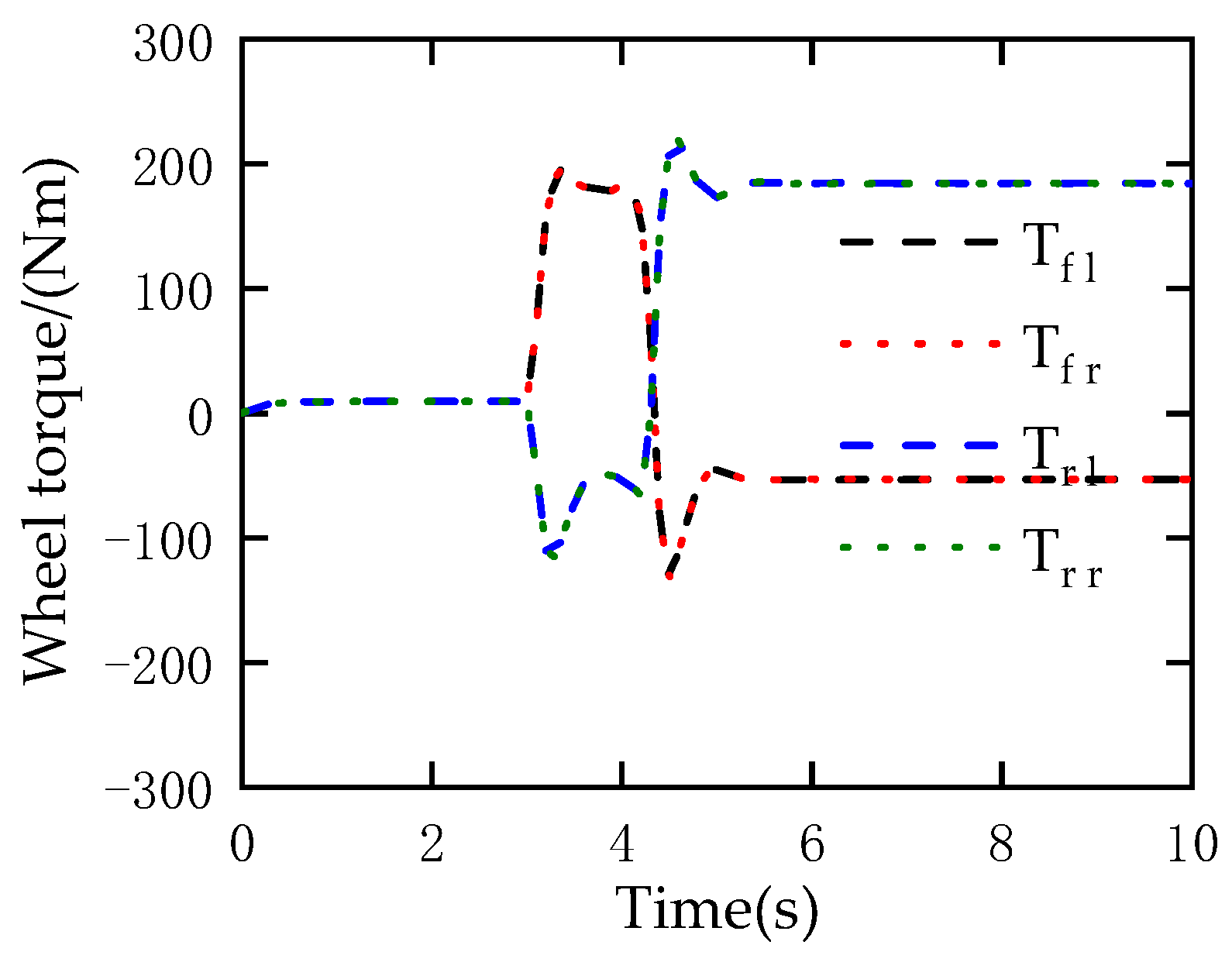
The output torque of the wheels coordinated by DC is shown in Figure 29. By assigning the torque to four wheels, a compensated yaw, roll, and pitch moment is formed, which enables the vehicle to quickly enter the steady state and improves the stability of the vehicle.
4.2. Fish Hook Working Condition
The vehicle was tested at an initial speed of and a road adhesion coefficient of 0.4. The fishhook working condition can better reflect the response characteristics of the vehicle under emergency obstacle avoidance operation, which can further verify the control effect of the designed control system on vehicle stability and drive-brake stability.
The dynamic response of the vehicle is shown in Figure 32, Figure 33, Figure 34, Figure 35, Figure 36 and Figure 37. The vehicle speed, lateral acceleration, yaw rate, side slip angle, roll angle, and pitch angle of the uncontrolled vehicle have a large overshoot. Also, the vehicle is unstable, and the trajectory has obvious deviation.
After applying the control, both control strategies ensure the yaw stability of the vehicle, but the vehicle with YSDC exhibits better-desired value tracking in the yaw rate response compared to the vehicle with NYSC, which is smoother and ensures a smaller amplitude of the side slip angle to keep the vehicle trajectory close to the desired path.
The speed of the vehicle loaded with NYSC is significantly reduced, and the body movement is increased. Even if the yaw movement is effectively suppressed, the violent movement of the body may cause the vehicle to roll over. The vehicle with YSDC has a more stable speed and effectively reduces body movement, which can ensure the vehicle’s yaw stability while taking into account the body stability and enhancing the overall spatial stability of the vehicle.
Figure 38, Figure 39, Figure 40 and Figure 41 show the longitudinal slip rate of the wheels. During the steering phase, the braking slip rate of the left wheel of the vehicle, without considering the slip constraint, exceeds the desired slip rate region, the magnitude exceeds −0.5 (50%), and the tire operates in an unstable condition. However, in contrast, the slip rate of the vehicle loaded with YSDC can be well controlled within the desired slip rate, allowing the vehicle to make fuller use of the tire adhesion and ensuring that the tire can provide a stable tire force. The solved optimal torque output signal is shown in Figure 42.
5. Conclusions
- (1)
- The research revolves around the distributed vehicle motion coupling problem and proposes a multi-objective constraint-based traverse stability decoupling control strategy. In the objective function design of the controller, the objective is to improve the vehicle driving stability and to optimize the vehicle speed and wheel slip rate with constraints. The torque coordination control is carried out through a quadratic planning method based on the minimum tire utilization rate to ensure the tires work in the stable region and improve the stability of driving/braking.
- (2)
- Through the test, the key parameters of the vehicle’s dynamic characteristics were identified, and the Carsim vehicle system was customized. The vehicle Carsim model was established, and the validity of the vehicle model was verified based on the vehicle handling stability test.
- (3)
- In this paper, two simulation conditions are designed to experimentally verify the effectiveness of the proposed control strategy. The results show that the proposed decoupled control strategy can not only effectively track the desired yaw rate and side slip angle response but also improve the stability of the body, effectively ensure the stability of the vehicle speed, and control the wheel slip rate within the desired range during the driving process of the vehicle. This strategy effectively improves the spatial stability and safety of the vehicle.
- (4)
- In this article, the spatial motion decoupling control for distributed-drive electric vehicles has a better control effect, but the response efficiency and energy loss of the actual motor are not considered, and further control studies combining generator response efficiency, energy management, and driving stability are needed.
Author Contributions
W.W., Z.L. and S.Y. provided the research proposal, research design, methodology selection, and construction of the simulation model in MATLAB/sinulink; S.Y., X.S. and Y.Q. assisted in data collection, processing, and analysis; F.L. participated in writing and revising the paper. All authors have read and agreed to the published version of the manuscript.
Funding
Research on modeling and control strategy of lateral stability of high ground clearance sprayer: ZZ202401; National Natural Science Foundation of China: 2020D01B23.
Data Availability Statement
The datasets presented in this article are not readily available because [The project is in a confidential phase as it has not yet been finalized]. Requests to access the datasets should be directed to [Contact the author’s email: [email protected]].
Conflicts of Interest
The authors declare no conflict of interest.
References
- Hu, J.-S.; Yin, D.; Hori, Y.; Hu, F.-R. Electric Vehicle Traction Control: A New MTTE Methodology. IEEE Ind. Appl. Mag. 2012, 18, 23–31. [Google Scholar] [CrossRef]
- Dadashnialehi, A.; Bab-Hadiashar, A.; Cao, Z.; Kapoor, A. Intelligent Sensorless ABS for In-Wheel Electric Vehicles. IEEE Trans. Ind. Electron. 2014, 61, 1957–1969. [Google Scholar] [CrossRef]
- Wang, J.; Wang, Q.; Jin, L.; Song, C. Independent wheel torque control of 4WD electric vehicle for differential drive assisted steering. Mechatronics 2011, 21, 63–76. [Google Scholar] [CrossRef]
- Falkner, A.; Reinalter, W. Consistent vehicle model for determining the design envelope, ride comfort and component load. Veh. Syst. Dyn. 2006, 44, 468–478. [Google Scholar] [CrossRef]
- Zhang, C.; Ma, J.; Chang, B.; Wang, J. Research on Anti-Skid Control Strategy for Four-Wheel Independent Drive Electric Vehicle. World Electr. Veh. J. 2021, 12, 150. [Google Scholar] [CrossRef]
- Al Kamil Safa, J.D.; Llamas, S. Design All-Wheel Drive Vehicles Based on Differential Speed Control Systems. Mechatron. Syst. Control 2021, 49, 25–26. [Google Scholar] [CrossRef]
- Zhao, J.; Wang, Y. Analysis and research on wheel steering motion of four-wheel locomotive. J. Phys. Conf. Ser. 2020, 1545, 012010. [Google Scholar] [CrossRef]
- Liao, Z.; Cai, L.; Yang, Q.; Zhang, Y. Design of lateral dynamic control objectives for multi-wheeled distributed drive electric vehicles. Eng. Sci. Technol. Int. J. 2024, 50, 101629. [Google Scholar] [CrossRef]
- Ribeiro, A.M.; Fioravanti, A.R.; Moutinho, A.; de Paiva, E.C. Nonlinear state-feedback design for vehicle lateral control using sum-of-squares programming. Veh. Syst. Dyn. 2022, 60, 743–769. [Google Scholar] [CrossRef]
- Wang, J.; Zhang, C.; Yang, Z.; Dang, M.; Chang, B.; Li, C.; Zhang, R.; Ma, J. Hierarchical driving force allocation strategy for 4-WID electric vehicles. Proc. Inst. Mech. Eng. Part D J. Automob. Eng. 2023, 10, 237. [Google Scholar] [CrossRef]
- Zhang, W.; Wang, Z.; Drugge, L.; Nybacka, M. Evaluating Model Predictive Path Following and Yaw Stability Controllers for Over-Actuated Autonomous Electric Vehicles. IEEE Trans. Veh. Technol. 2020, 69, 1109. [Google Scholar] [CrossRef]
- Yang, K.; Dong, D.; Ma, C.; Tian, Z.; Chang, Y.; Wang, G. Stability control for electric vehicles with four in-wheel-motors based on sideslip angle. World Electr. Veh. J. 2021, 12, 42. [Google Scholar] [CrossRef]
- Motoki, S.; Gaku, Y.; Daisuke, G.; Takehiro, I.; Hiroshi, F. Development of Wireless In-Wheel Motor Using Magnetic Resonance Coupling. IEEE Trans. Power Electron. 2016, 31, 5270–5278. [Google Scholar]
- Luque, P.; Mántaras, D.A.; Maradona, Á.; Roces, J.; Sánchez, L.; Castejón, L.; Malón, H. Multi-Objective Evolutionary Design of an Electric Vehicle Chassis. Sensors 2020, 20, 3633. [Google Scholar] [CrossRef] [PubMed]
- Liang, Y.; Müller, S.; Schwendner, D.; Rolle, D.; Schaffer, I. A Scalable Framework for Robust Vehicle State Estimation with a Fusion of a Low-Cost IMU, the GNSS, Radar, a Camera and Lidar. In Proceedings of the 2020 IEEE/RSJ International Conference on Intelligent Robots and Systems (IROS), Las Vegas, NV, USA, 25–29 October 2020; pp. 1661–1668. [Google Scholar] [CrossRef]
- Shahian Jahromi, B.; Tulabandhula, T.; Cetin, S. Real-Time Hybrid Multi-Sensor Fusion Framework for Perception in Autonomous Vehicles. Sensors 2019, 19, 4357. [Google Scholar] [CrossRef] [PubMed]
- Tian, D.; Jin, L.; Zhang, Z.; Li, H. Vehicle State Estimation Based on Multidimensional Information Fusion. IEEE Access 2022, 10, 76220–76232. [Google Scholar] [CrossRef]
- Yang, S.; Choi, M.; Han, S.; Choi, K.H.; Kim, K.S. 4D Radar-Camera Sensor Fusion for Robust Vehicle Pose Estimation in Foggy Environments. IEEE Access 2023, 12, 2169–3536. [Google Scholar] [CrossRef]
- Farag, W. Kalman-filter-based sensor fusion applied to road-objects detection and tracking for autonomous vehicles. Proc. Inst. Mech. Eng. Part I J. Syst. Control. Eng. 2021, 235, 1125–1138. [Google Scholar] [CrossRef]
- Gao, H.; Cheng, B.; Wang, J.; Li, K.; Zhao, J.I.; Li, D. Object classification using CNN-based fusion of vision and LIDAR in autonomous vehicle environment. IEEE Trans. Ind. Inform. 2018, 14, 4224–4231. [Google Scholar] [CrossRef]
- Desjardins, C.; Chaib-Draa, B. Cooperative adaptive cruise control: A reinforcement learning approach. IEEE Trans. Intell. Transp. Syst. 2011, 12, 1248–1260. [Google Scholar] [CrossRef]
- Chong, L.; Abbas, M.M.; Flintsch, A.M.; Higgs, B. A rule-based neural network approach to model driver naturalistic behavior in traffic. Transp. Res. Part C Emerg. Technol. 2013, 32, 207–223. [Google Scholar] [CrossRef]
- Lin, J.; Zhang, P.; Li, C.; Zhou, Y.; Wang, H.; Zou, X. APF-DPPO: An Automatic Driving Policy Learning Method Based on the Artificial Potential Field Method to Optimize the Reward Function. Machines 2022, 10, 533. [Google Scholar] [CrossRef]
- Kumar, G.A.; Lee, J.H.; Hwang, J.; Park, J.; Youn, S.H.; Kwon, S. LiDAR and Camera Fusion Approach for Object Distance Estimation in Self-Driving Vehicles. Symmetry 2020, 12, 324. [Google Scholar] [CrossRef]
- Gao, F.; Duan, J.; Han, Z.; He, Y. Automatic virtual test technology for intelligent driving systems considering both coverage and efficiency. IEEE Trans. Veh. Technol. 2020, 69, 14365–14376. [Google Scholar] [CrossRef]
- Fan, P.; Khan, Z.; Abbas, F. A Novel Low-Latency V2V Resource Allocation Scheme Based on Cellular V2X Communications. IEEE Trans. Intell. Transp. Syst. 2019, 20, 2185–2197. [Google Scholar]
- Gao, H.; Liu, C.; Li, Y.; Yang, X. V2VR: Reliable Hybrid-Network-Oriented V2V Data Transmission and Routing Considering RSUs and Connectivity Probability. IEEE Trans. Intell. Transp. Syst. 2020, 22, 3533–3546. [Google Scholar] [CrossRef]
- Sun, C.; Vianney, J.M.U.; Li, Y.; Chen, L.; Li, L.I.; Wang, F.-Y.; Khajepour, A.; Cao, D. Proximity based automatic data annotation for autonomous driving. IEEE/CAA J. Autom. Sin. 2020, 7, 395–404. [Google Scholar] [CrossRef]
- Nam, K.; Fujimoto, H.; Hori, Y. Lateral Stability Control of In-Wheel-Motor-Driven Electric Vehicles Based on Sideslip Angle Estimation Using Lateral Tire Force Sensors. IEEE Trans. Veh. Technol. 2012, 61, 1972–1985. [Google Scholar]
- Guo, N.; Lenzo, B.; Zhang, X.; Zou, Y.; Zhai, R.; Zhang, T. A Real-time Nonlinear Model Predictive Controller for Yaw Motion Optimization of Distributed Drive Electric Vehicles. IEEE Trans. Veh. Technol. 2020, 69, 4935–4946. [Google Scholar] [CrossRef]
- Zhou, H.; Jia, F.; Jing, H.; Liu, Z.; Guvenc, L. Coordinated longitudinal and lateral motion control for four wheel independent motor-drive electric vehicle. IEEE Trans. Veh. Technol. 2018, 5, 3782–3790. [Google Scholar] [CrossRef]
- Atael, M.; Khajepou, A.; Jeon, S. Model predictive control for integrated lateral stability, traction /braking control, and rollover prevention of electric vehicles. Veh. Syst. Dyn. 2020, 58, 49–73. [Google Scholar]
- Liang, Y.; Li, Y.; Yu, Y.; Zheng, L. Integrated lateral control for 4WID/4WIS vehicle in high-speed condition considering the magnitude of steering. Vehicle. System. Dynamics. 2019, 1–25. [Google Scholar] [CrossRef]
- Huang, G.; Yuan, X.; Shi, K.; Wu, X. A BP-PID controller-based multi-model control system for lateral stability of distributed drive electric vehicle. J. Frankl. Inst. 2019, 13, 7290–7331. [Google Scholar] [CrossRef]
- Katsuyama, E. Decoupled 3D moment control using in-wheel motors. Veh. Syst. Dyn. 2013, 51, 18–31. [Google Scholar] [CrossRef]
- Cespi, R.; Galluzzi, R.; Ramirez-Mendoza, R.A.; Di Gennaro, S. Artificial Intelligence for Stability Control of Actuated In–Wheel Electric Vehicles with CarSim® Validation. Mathematics 2021, 9, 3120. [Google Scholar] [CrossRef]
- Wei, H.; Zhang, N.; Liang, J.; Ai, Q.; Zhao, W.; Huang, T.; Zhang, Y. Deep reinforcement learning based direct torque control strategy for distributed drive electric vehicles considering active safety and energy saving performance. Energy 2022, 238, 8. [Google Scholar] [CrossRef]
- Alsabbagh, A.; Wu, X.; Ma, C. Distributed Electric Vehicles Charging Management Considering Time Anxiety and Customer Behaviors. IEEE Trans. Ind. Inform. 2020, 17, 2422–2431. [Google Scholar] [CrossRef]
- Zhu, Z.D.Y. Thermo-mechanical coupled modeling for numerical analyzing the influence of thermal and frictional factors on the cornering behaviors of non-pneumatic mechanical elastic wheel. Simul. Model. Pract. Theory 2019, 91, 13–27. [Google Scholar] [CrossRef]
- Liang, D.; Wang, H.; Geng, N.; Lu, Y. Experimental study and analysis of automobile steering transient response. China Automob. 2020, 5. [Google Scholar]
- Zhao, Y.; Deng, H.; Li, Y.; Xu, H. Coordinated control of stability and economy based on torque distribution of distributed drive electric vehicle. Proc. Inst. Mech. Eng. Part D J. Automob. Eng. 2020, 234, 1792–1806. [Google Scholar] [CrossRef]
- Yang, S.; Feng, J.; Song, B. Research on Decoupled Optimal Control of Straight-Line Driving Stability of Electric Vehicles Driven by Four-Wheel Hub Motors. Energies 2021, 18, 5766. [Google Scholar] [CrossRef]
- Wang, Q.; Zhao, Y.; Xie, W.; Zhao, Q.; Lin, F. Hierarchical estimation of vehicle state and tire forces for distributed in-wheel motor drive electric vehicle without previously established tire model. J. Frankl. Inst. 2022, 359, 7051–7068. [Google Scholar] [CrossRef]
- Sun, W.; Chen, Y.; Wang, J.; Wang, X.; Liu, L. Research on TVD Control of Cornering Energy Consumption for Distributed Drive Electric Vehicles Based on PMP. Energies 2022, 15, 2641. [Google Scholar] [CrossRef]
- Zhang, N.; Wang, J.; Li, Z.; Li, S.; Ding, H. Multi-Agent-Based Coordinated Control of ABS and AFS for Distributed Drive Electric Vehicles. Energies 2022, 15, 1919. [Google Scholar] [CrossRef]
- Zou, Y.; Guo, N.; Zhang, X. An integrated control strategy of path following and lateral motion stabilization for autonomous distributed drive electric vehicles. Proc. Inst. Mech. Eng. Part D J. Automob. Eng. 2019, 235, 1164–1179. [Google Scholar] [CrossRef]
- Wu, Z.; Chen, B. Distributed Electric Vehicle Charging Scheduling with Transactive Energy Management. Energies 2022, 15, 163. [Google Scholar] [CrossRef]
- Małek, A.; Caban, J.; Dudziak, A.; Marciniak, A.; Ignaciuk, P. A Method of Assessing the Selection of Carport Power for an Electric Vehicle Using the Metalog Probability Distribution Family. Energies 2023, 16, 5077. [Google Scholar] [CrossRef]
- Pipeleers, G.; Demeulenaere, B.; Swevers, J.; Vandenberghe, L. Extended LMI characterizations for stability and performance of linear systems. Syst. Control Lett. 2009, 7, 510–518. [Google Scholar] [CrossRef]
- Li, Y.; Zhang, S.; Pan, Y.; Zhou, B.; Peng, Y. Exploring the Stability and Capacity Characteristics of Mixed Traffic Flow with Autonomous and Human-Driven Vehicles considering Aggressive Driving. J. Adv. Transp. 2023, 2023, 2578690. [Google Scholar] [CrossRef]
- Qi, J. Development and Validation of Electronic Stability Control System Algorithm Based on Tire Force Observation. Appl. Sci. 2020, 10, 8741. [Google Scholar]
Figure 1.
Distributed electric vehicle driving force analysis diagram. Gray arrow is the tire driving force when driving, black arrow is the tire braking force when braking.
Figure 1.
Distributed electric vehicle driving force analysis diagram. Gray arrow is the tire driving force when driving, black arrow is the tire braking force when braking.
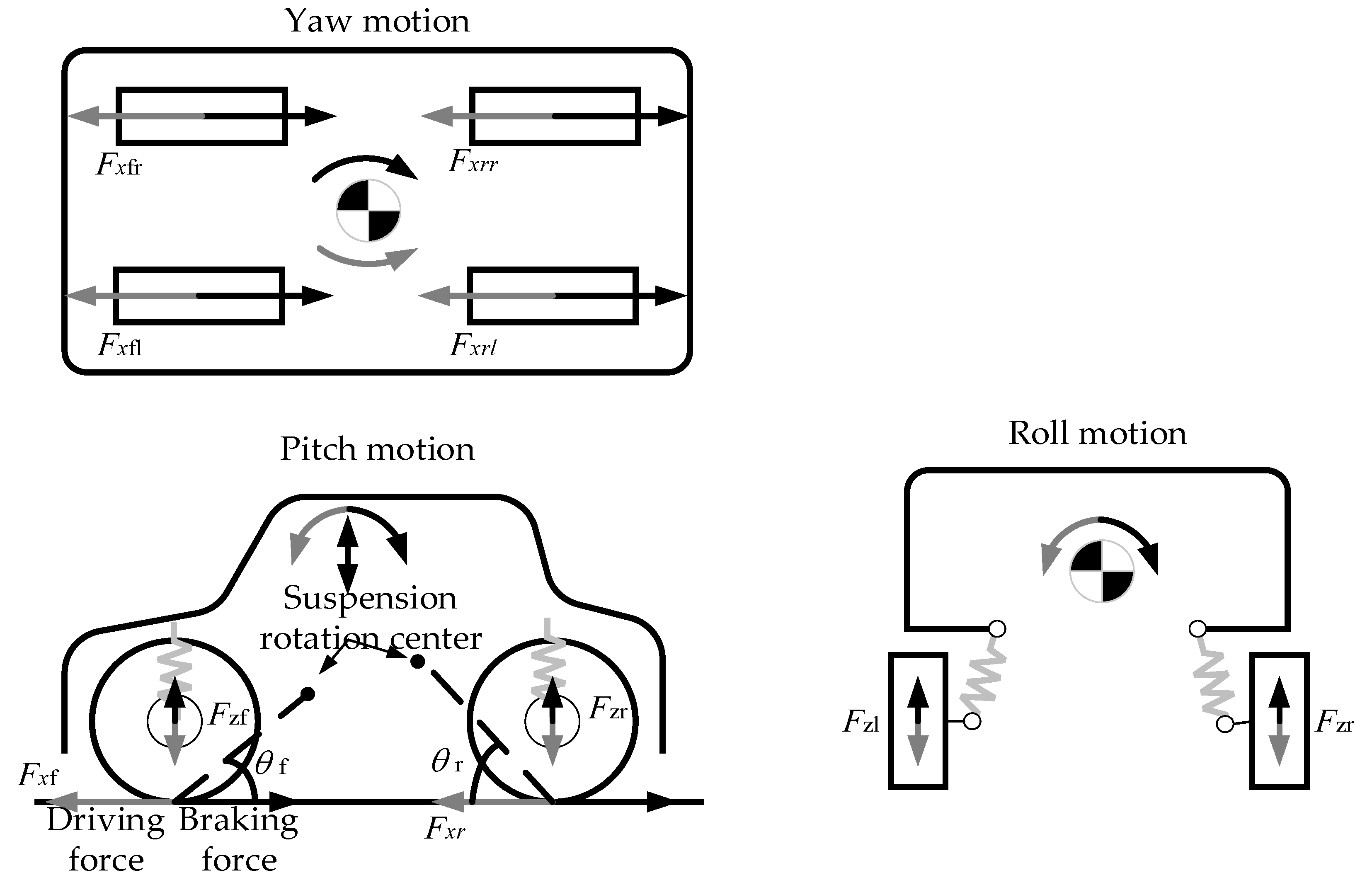
Figure 2.
Coasting test longitudinal speed at initial speed 35 km/h.

Figure 3.
Coasting test longitudinal speed at initial speed 70 km/h.
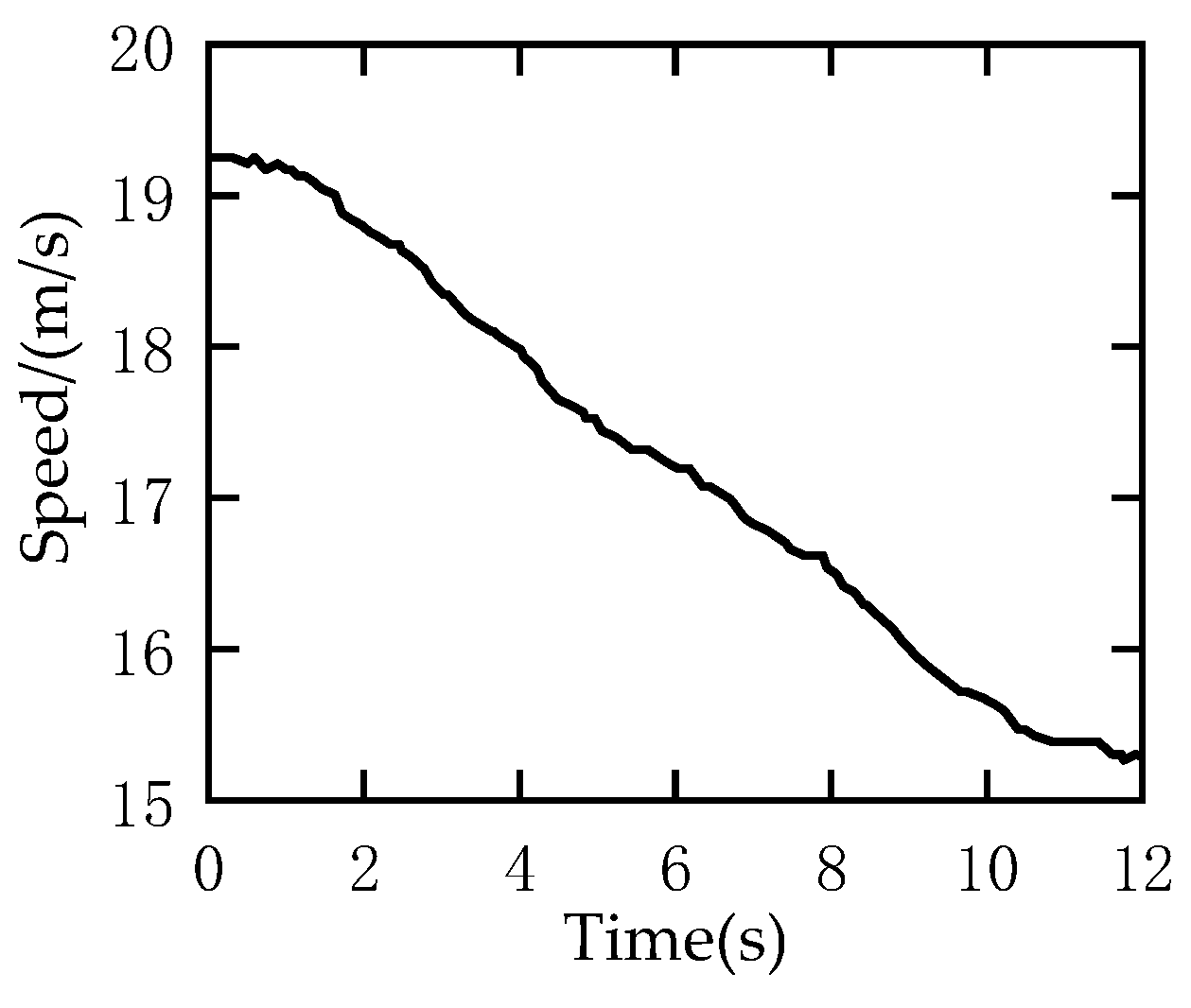
Figure 4.
The relationship between steering wheel angle and front-wheel angle.

Figure 5.
Front and rear axle slip angle.

Figure 6.
Front and rear axle lateral force.

Figure 7.
Front axle fitting results.
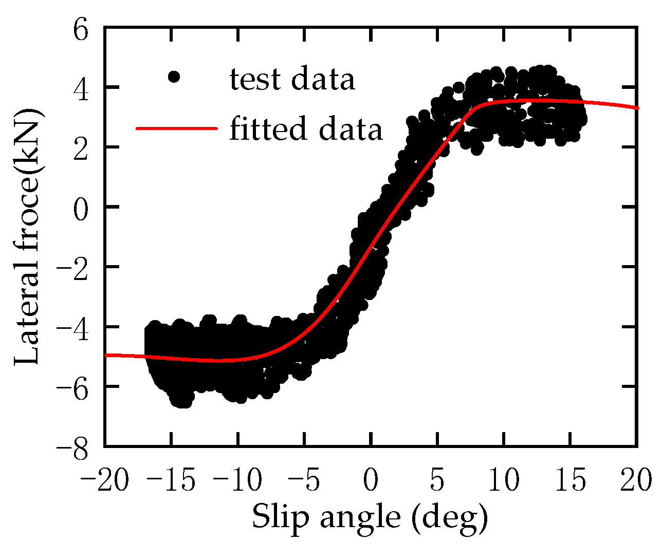
Figure 8.
Rear axle fitting results.
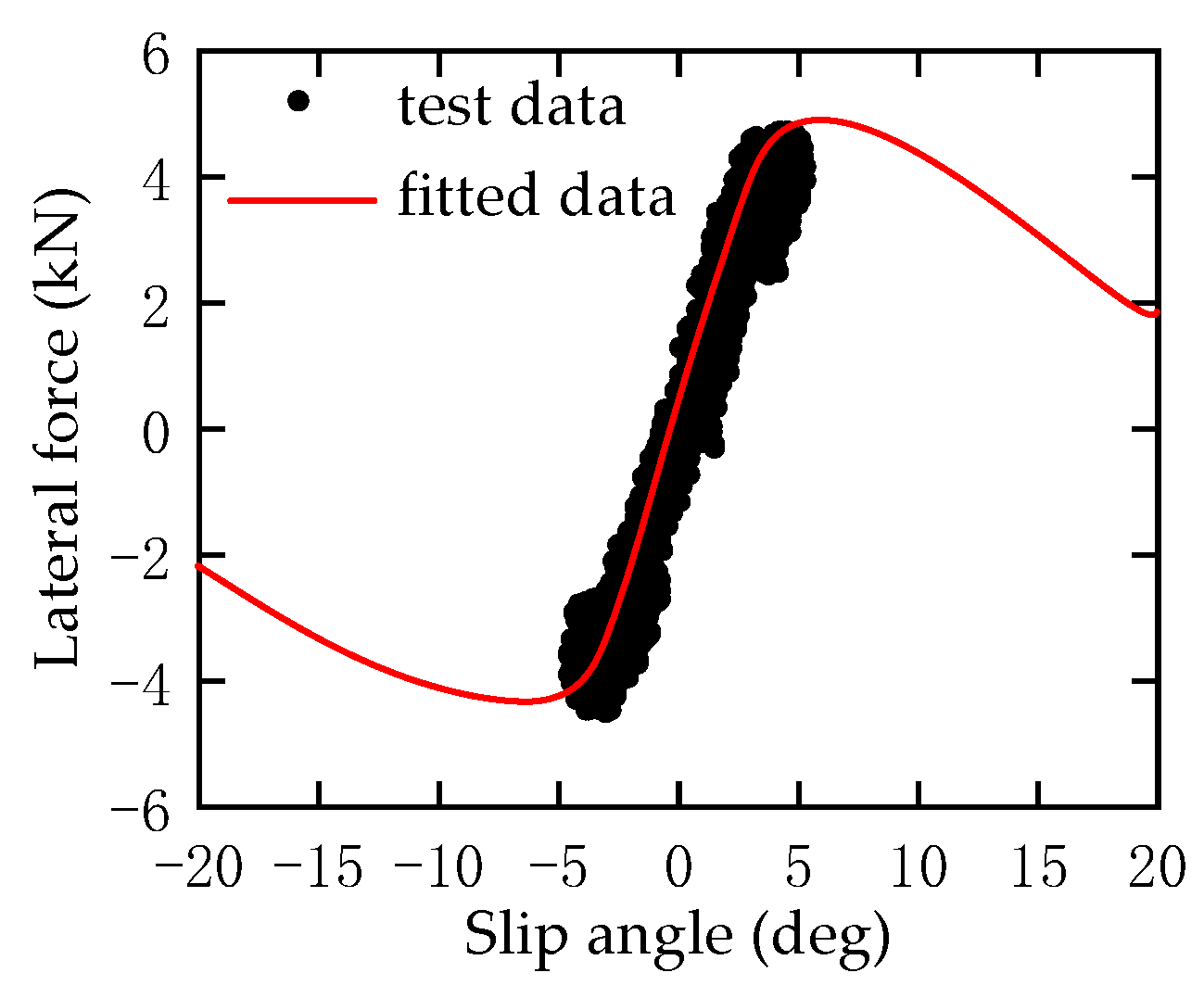
Figure 9.
Power and transmission system.
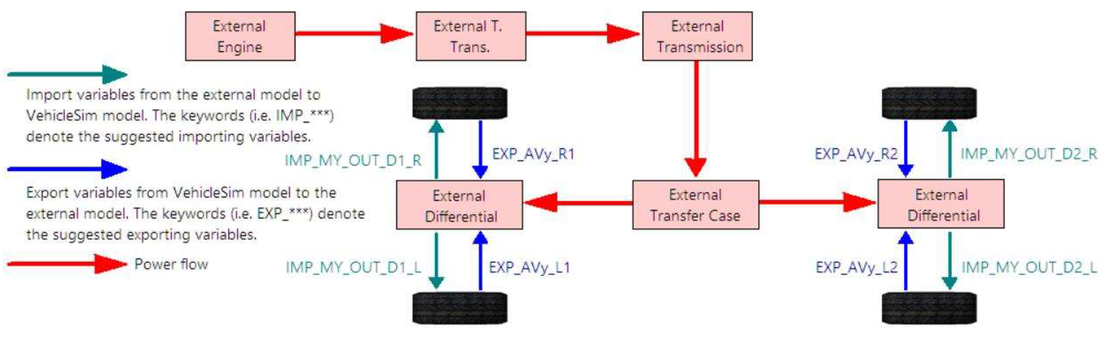
Figure 10.
Vehicle testing.
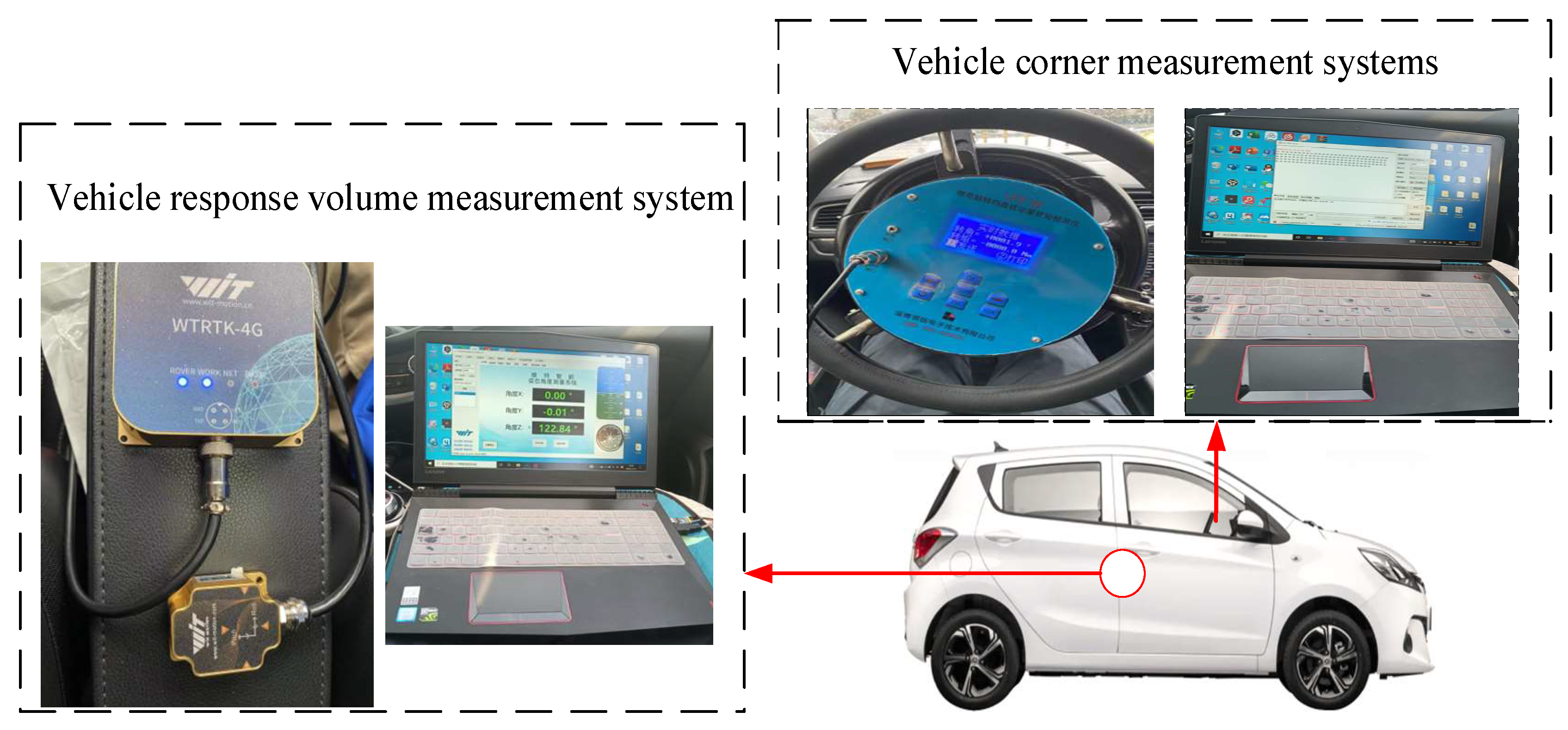
Figure 11.
Yaw rate.
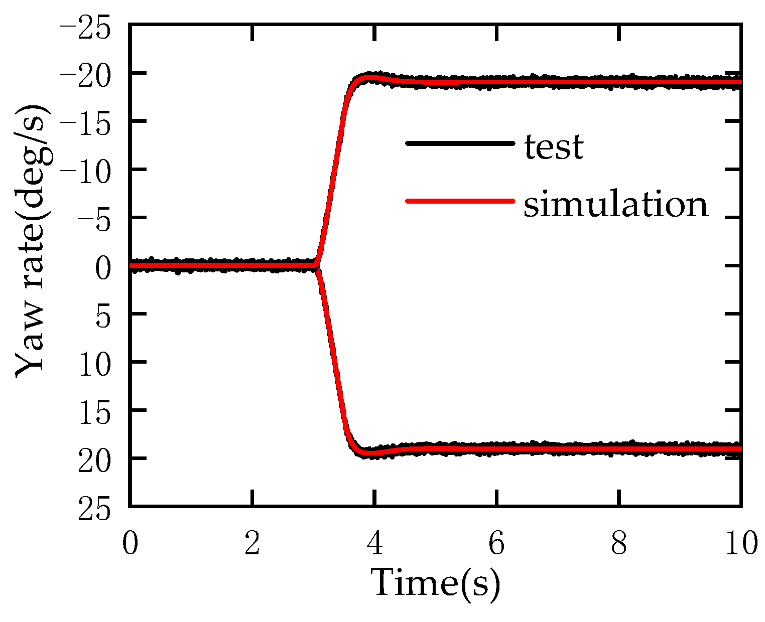
Figure 12.
Side slip angle.
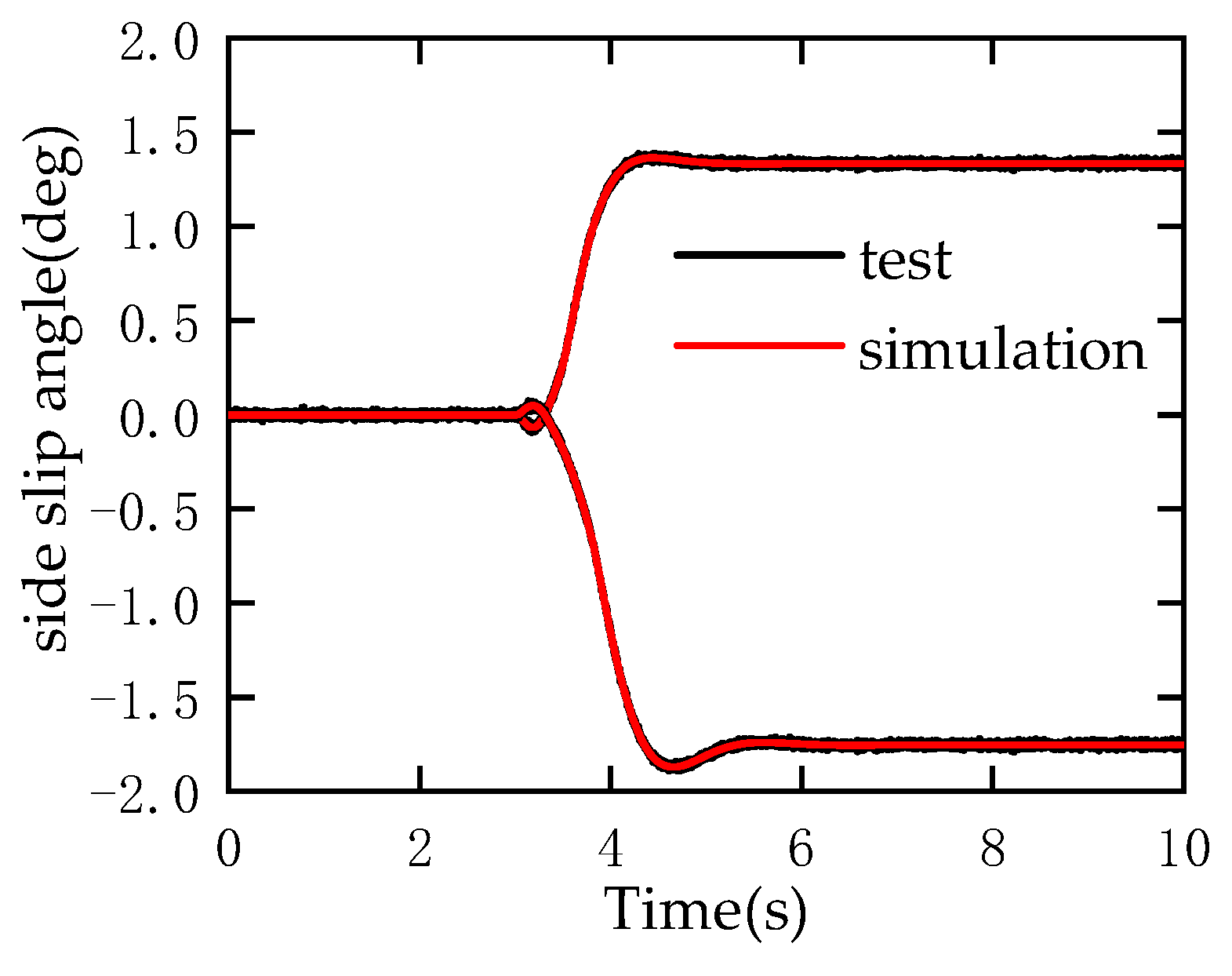
Figure 13.
Lateral acceleration.
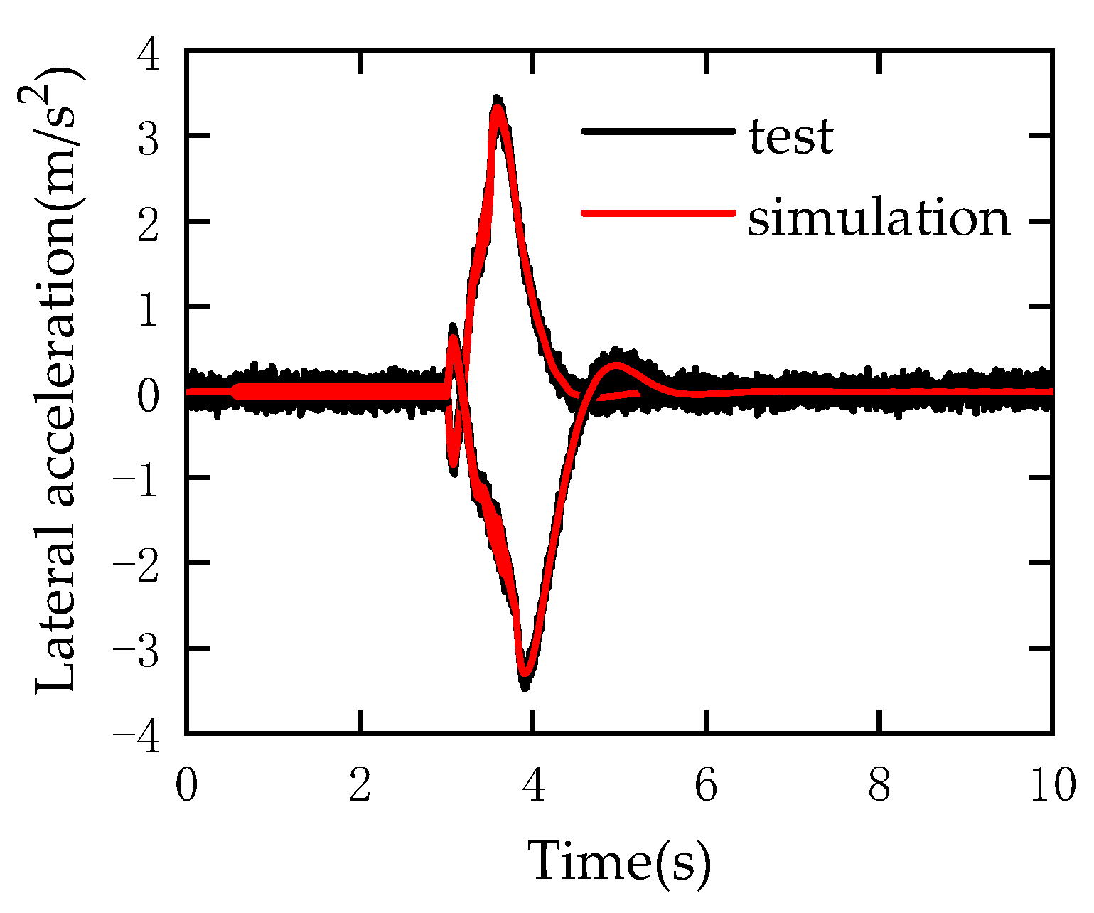
Figure 14.
Roll angle.

Figure 15.
Longitudinal plane motion analysis.

Figure 16.
Horizontal plane motion analysis.
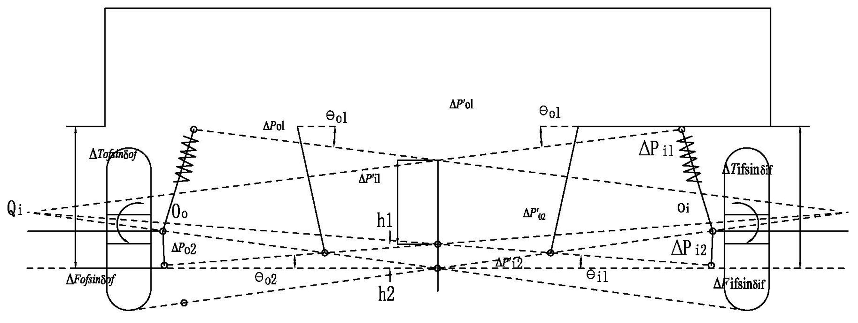
Figure 17.
Additional acceleration.
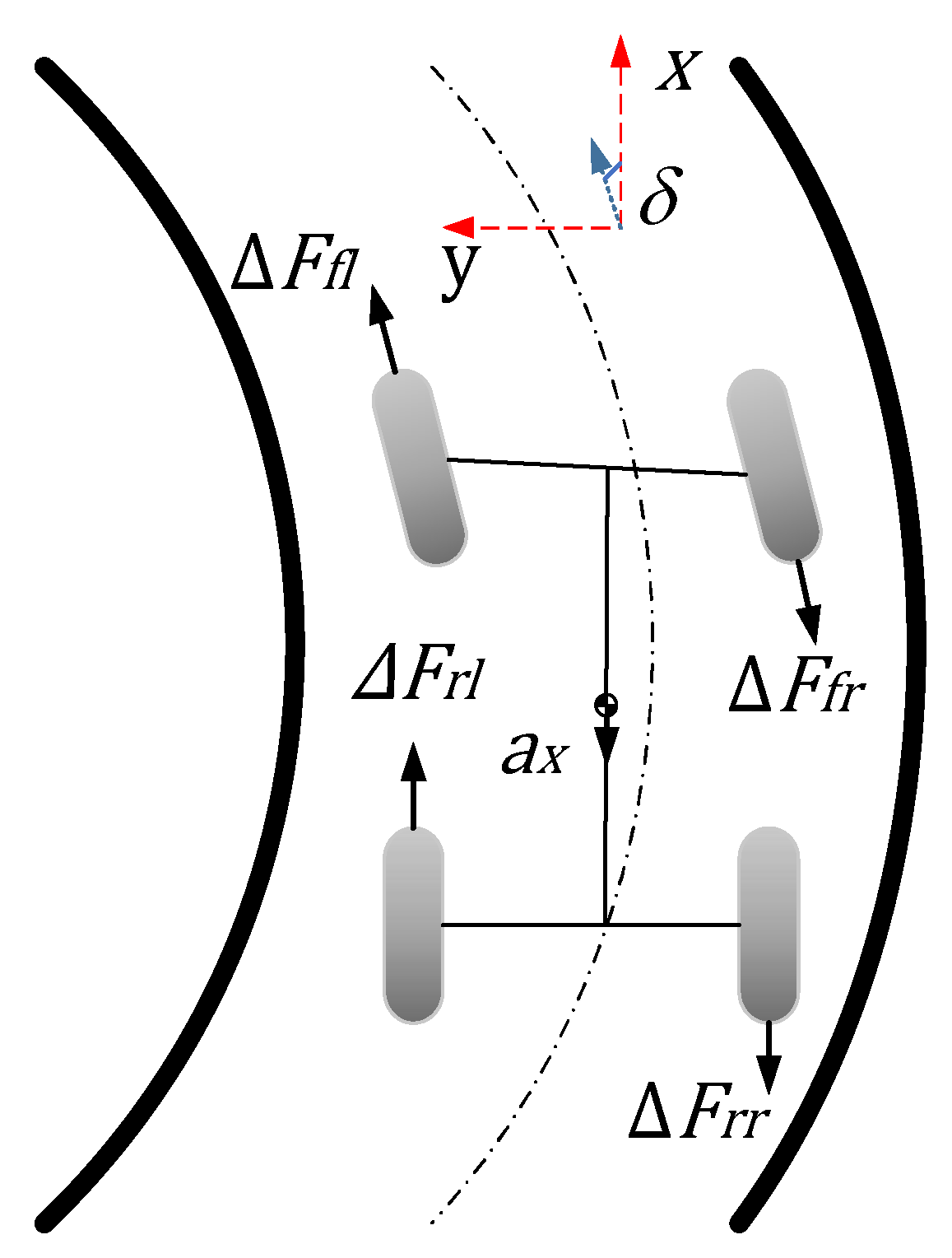
Figure 18.
Relationship between longitudinal force and slip rate.
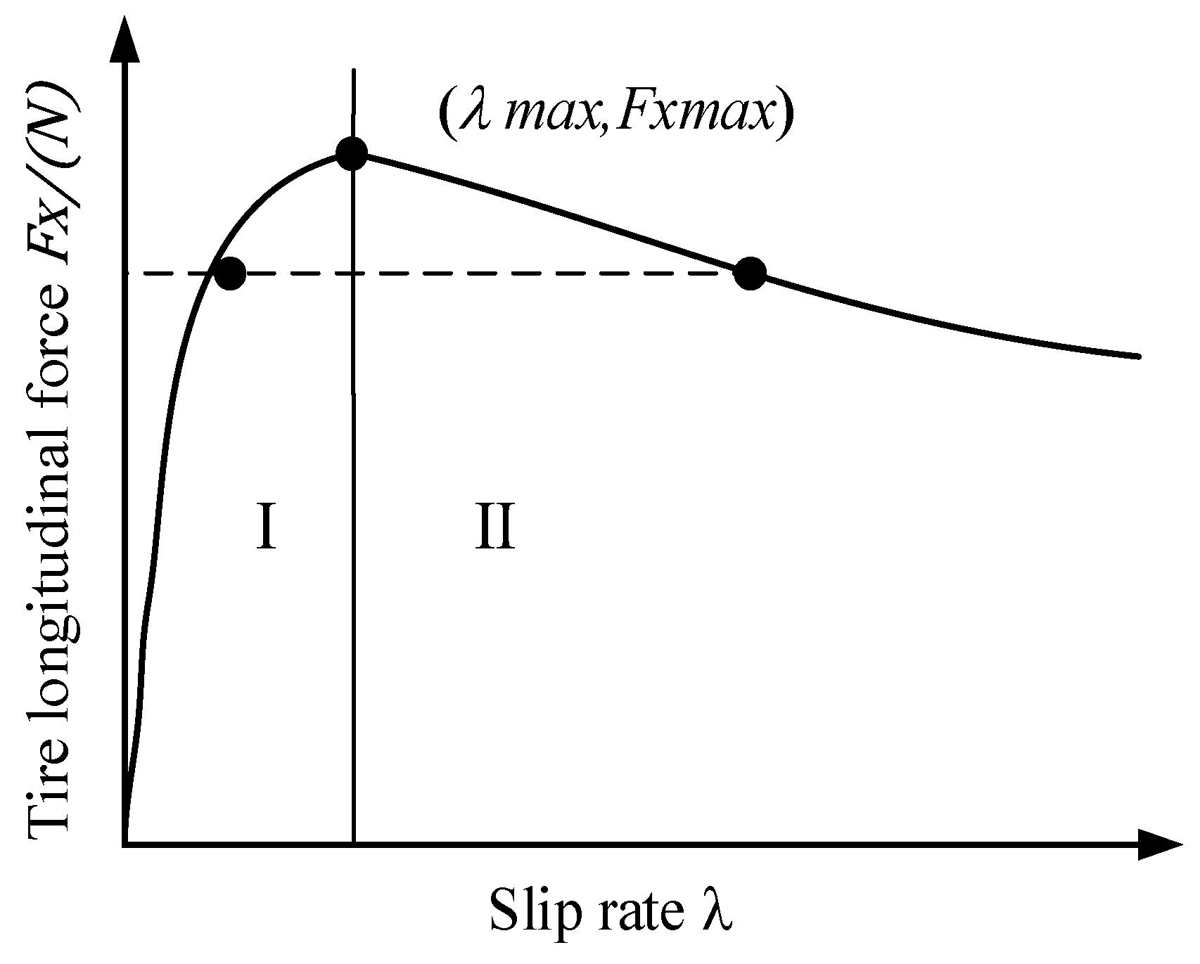
Figure 19.
Schematic diagram of tire adhesion ellipse.
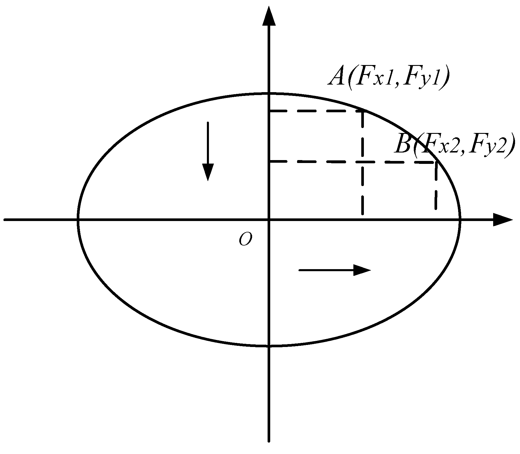
Figure 20.
Complete vehicle 2-degrees-of-freedom model.
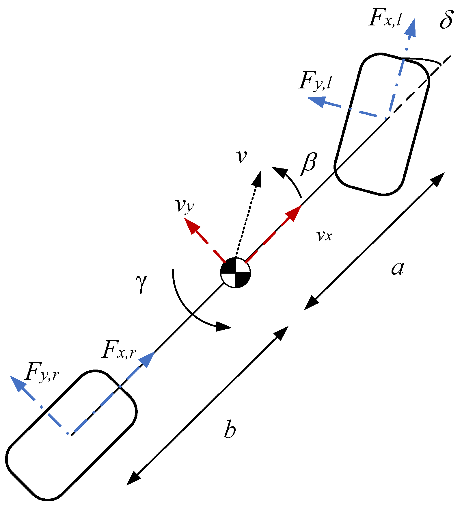
Figure 21.
Wheel steer angle.
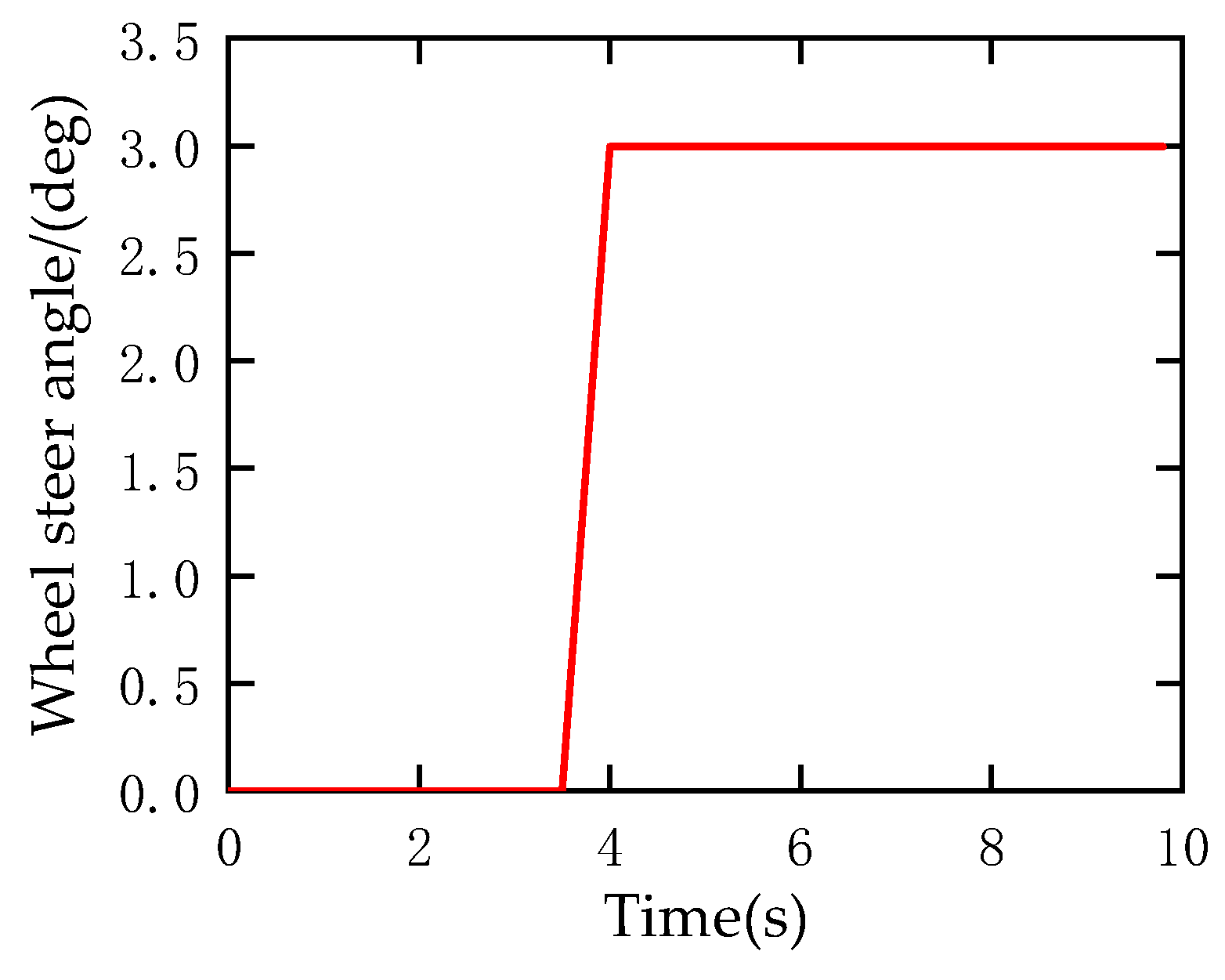
Figure 22.
Speed.

Figure 23.
Side slip angle.
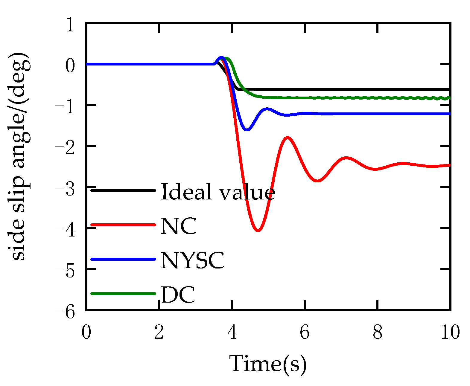
Figure 24.
Yaw rate.

Figure 25.
Roll angle.

Figure 26.
Pitch angle.
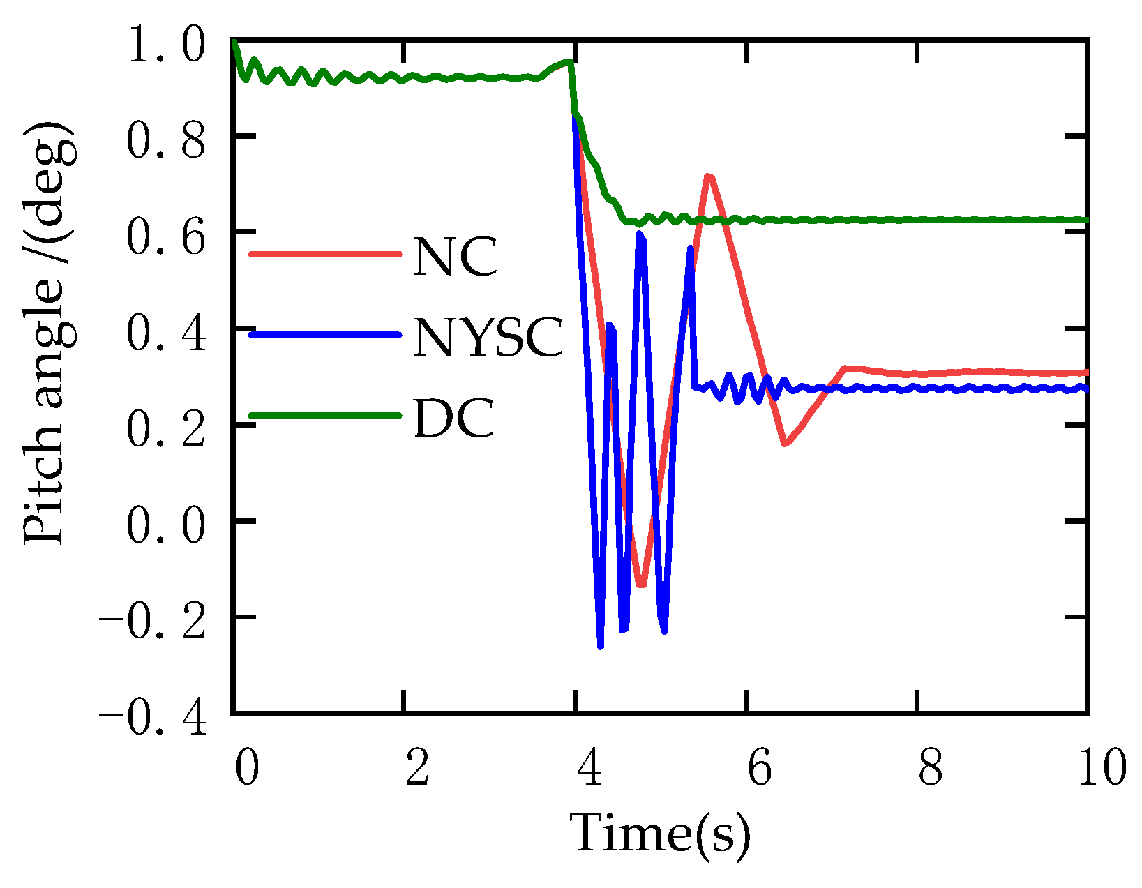
Figure 27.
Left front-wheel slip rate.
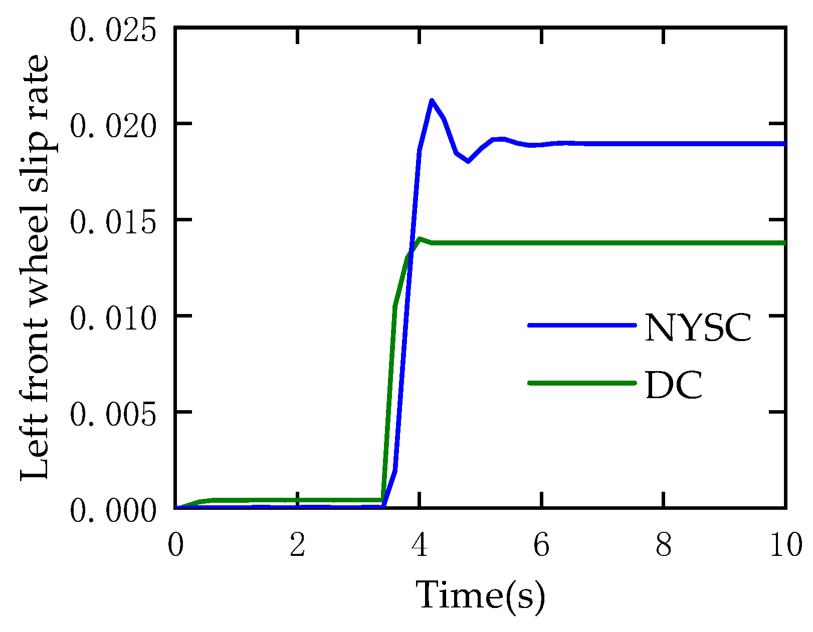
Figure 28.
Right front-wheel rate.

Figure 29.
Left rear-wheel rate.
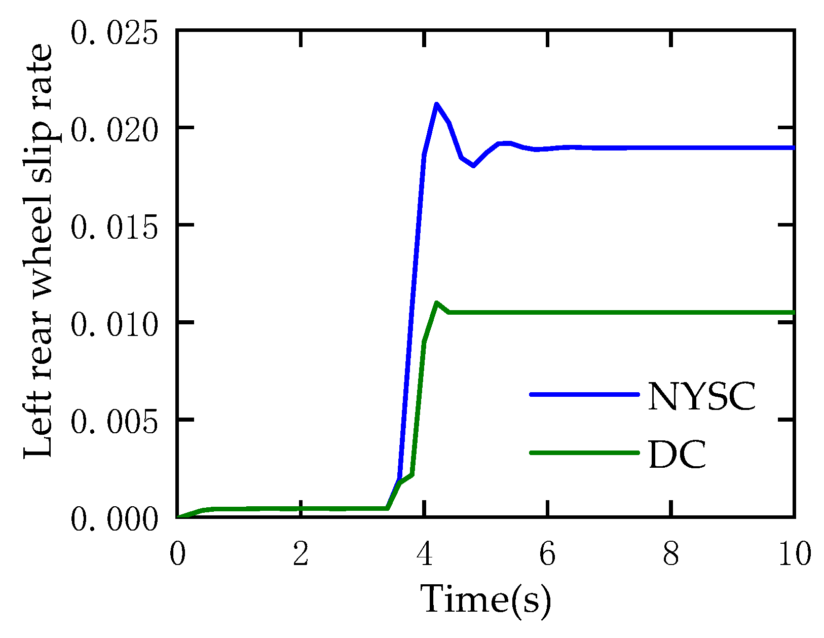
Figure 30.
Right rear-wheel rate.
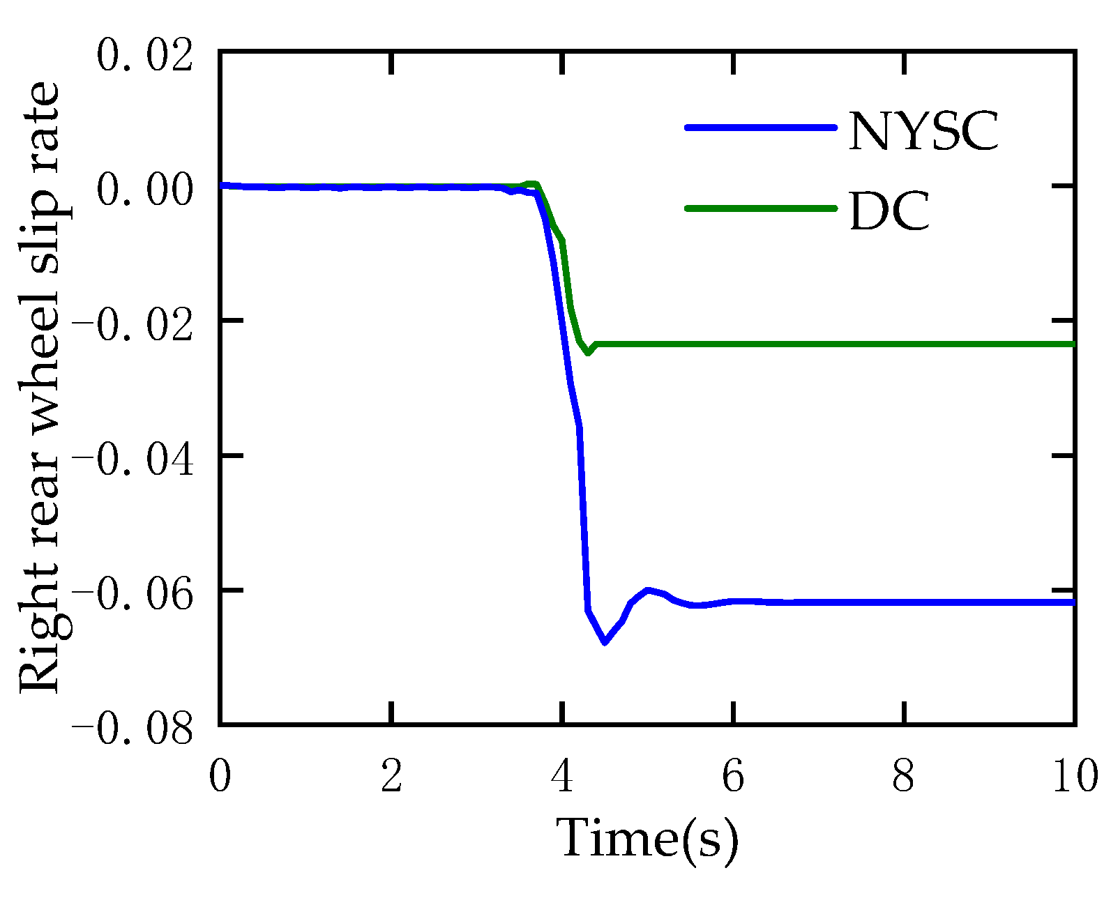
Figure 31.
Torque output of four wheels.
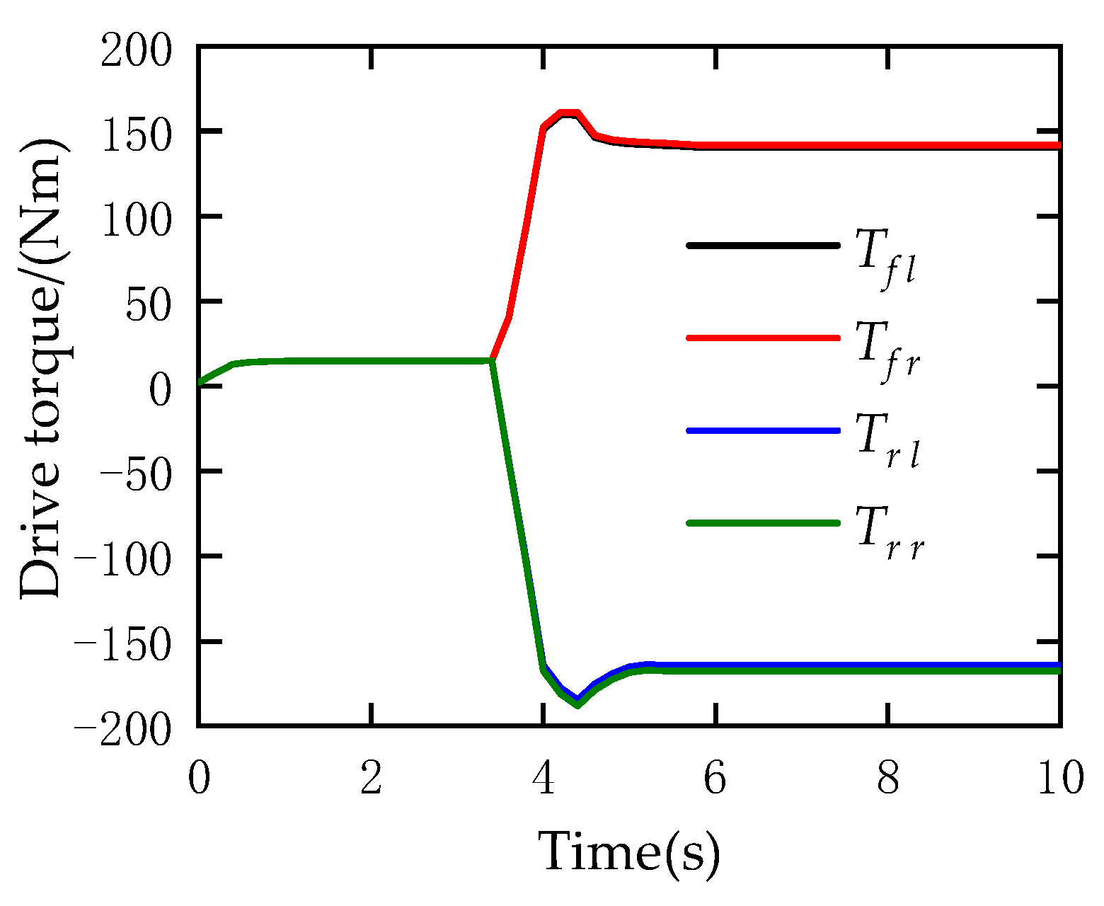
Figure 32.
Speed.
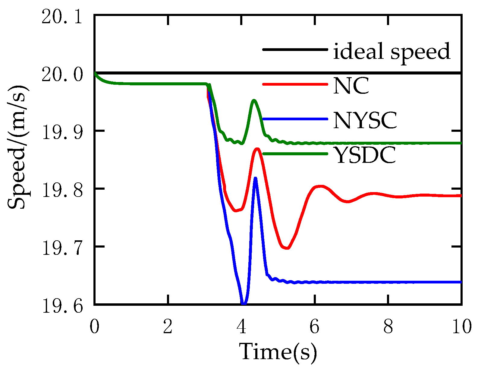
Figure 33.
Lateral acceleration.

Figure 34.
Yaw rate.

Figure 35.
Side slip rate.

Figure 36.
Roll angle.

Figure 37.
Pitch angle.
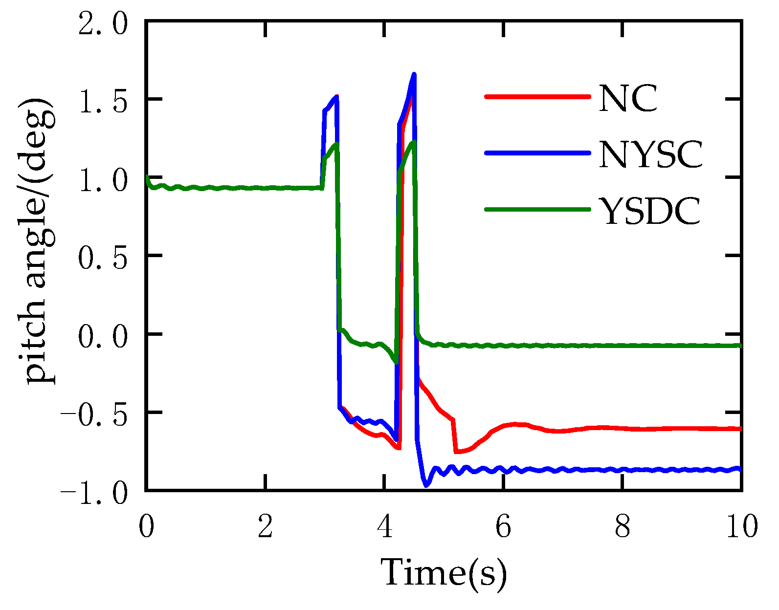
Figure 38.
Left front-wheel slip rate.
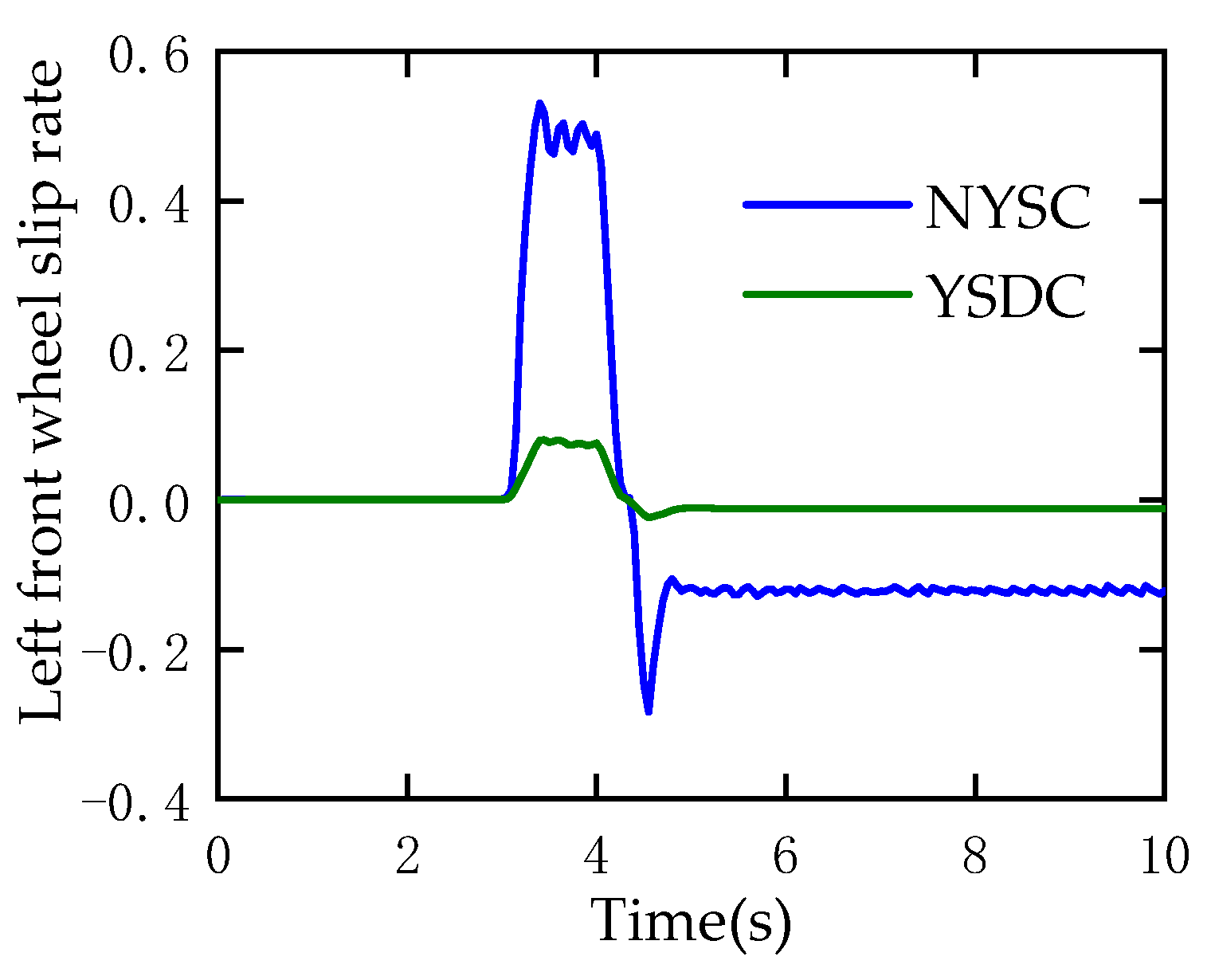
Figure 39.
Right front-wheel slip rate.
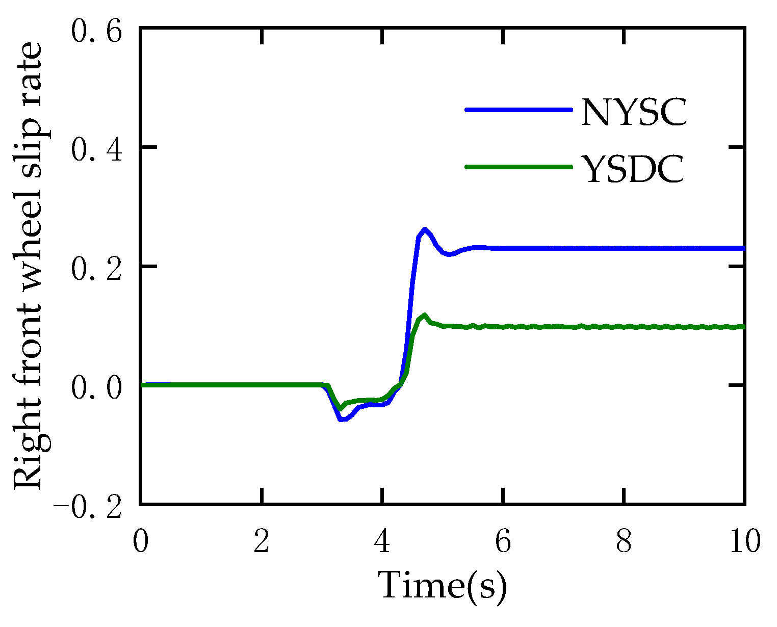
Figure 40.
Left rear-wheel slip rate.
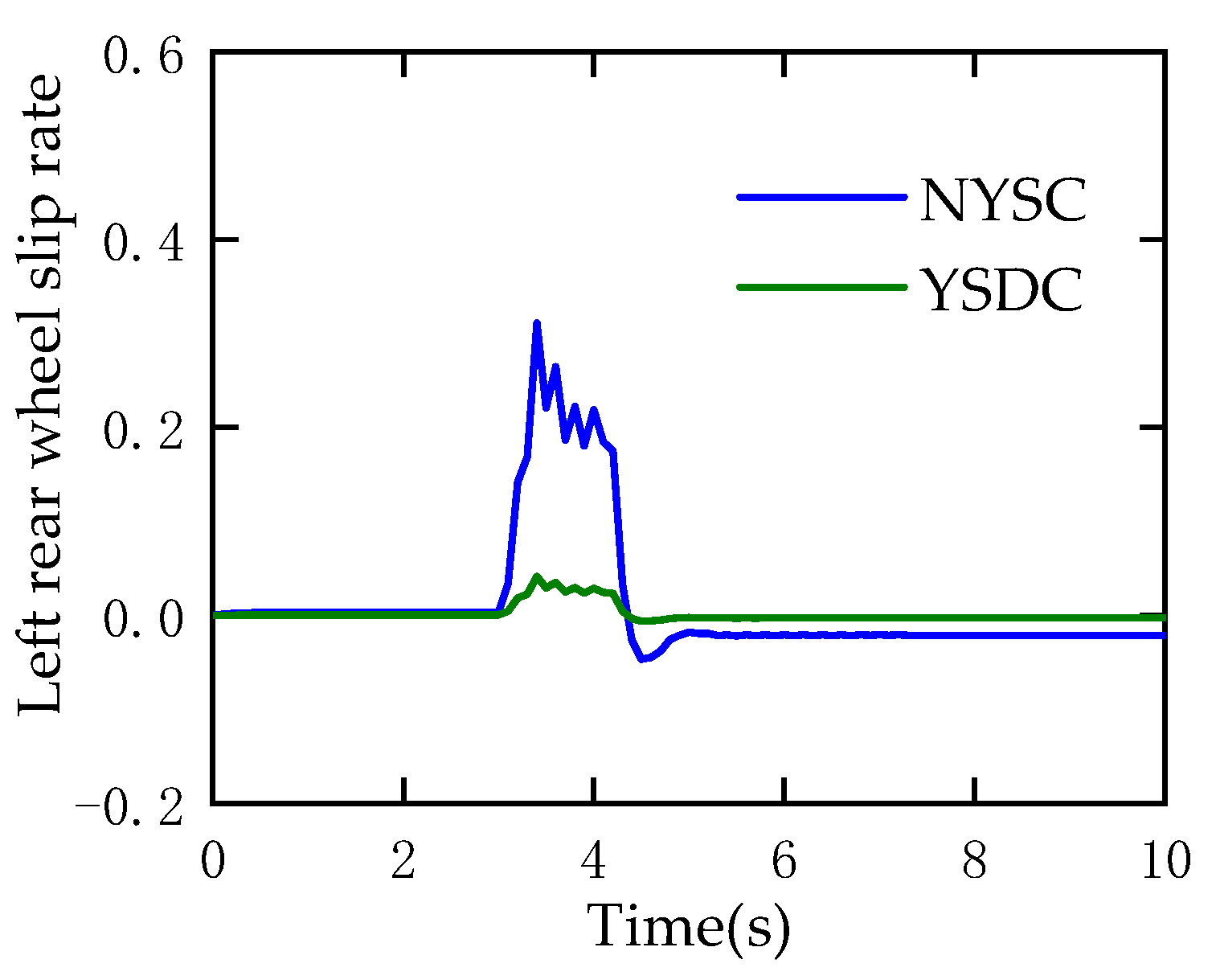
Figure 41.
Right rear-wheel slip rate.
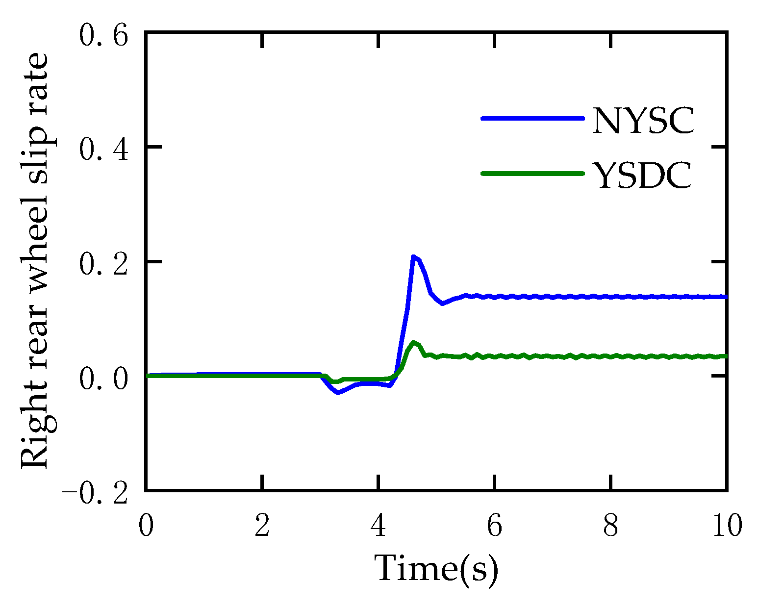
Figure 42.
Torque output of four wheels.

Table 1.
Nomenclature.
| Symbol | Physical Meaning | Unit |
|---|---|---|
| vehicle mass | kg | |
| Yaw rate | rad/s | |
| Distance from center of mass to front axis | m | |
| Distance from center of mass to rear axis | m | |
| Wheelbase | m | |
| Vehicle length | m | |
| Driver steering angle | deg | |
| Effective wheel radius | m | |
| Wheel longitudinal force | N | |
| Wheel Lateral force | N | |
| Tire-ground contact force | N | |
| Tread | m | |
| Wheel slip rate | / | |
| Vehicle side slip angle | deg | |
| Front-wheel lateral deflection stiffness | / | |
| Rear-wheel lateral deflection stiffness | / | |
| Longitudinal speed of the wheel | m/s | |
| Lateral speed of the wheel | m/s | |
| is front, is rear | / | |
| is left, is right | / | |
| Pavement adhesion coefficient | / |
Table 2.
Longitudinal vehicle speed and longitudinal acceleration under coasting test.
| Serial Number | Test Conditions | Longitudinal Speed (m/s) | Longitudinal Acceleration (m/s2) |
|---|---|---|---|
| 1 | 8.3677 | −0.1161 | |
| 2 | 8.3392 | −0.1061 | |
| 3 | 8.2828 | −0.1674 | |
| 4 | 18.1849 | −0.4637 | |
| 5 | 18.1027 | −0.3791 | |
| 6 | 18.0616 | −0.3477 |
Table 3.
Measured values for and .
| Data Portfolio | ||
|---|---|---|
| 1,4 | −63.17 | −1.66 |
| 1,5 | −70.13 | −1.62 |
| 1,6 | −69.67 | −1.59 |
| 2,4 | −68.97 | −1.63 |
| 2,5 | −69.37 | −1.56 |
| 2,6 | −76.16 | −1.58 |
| 3,4 | −83.18 | −1.62 |
| 3,5 | −89.23 | −1.51 |
| 3,6 | −90.12 | −1.52 |
Table 4.
Motor parameters.
| Motor Parameters | Value | Unit |
|---|---|---|
| Rated power | 14 | kW |
| Peak power | 28 | kW |
| Rated rotation speed | 800 | |
| Peak rotation speed | 1600 | |
| Rated torque | 145 | |
| Peak torque | 290 |
Disclaimer/Publisher’s Note: The statements, opinions and data contained in all publications are solely those of the individual author(s) and contributor(s) and not of MDPI and/or the editor(s). MDPI and/or the editor(s) disclaim responsibility for any injury to people or property resulting from any ideas, methods, instructions or products referred to in the content. |
© 2024 by the authors. Licensee MDPI, Basel, Switzerland. This article is an open access article distributed under the terms and conditions of the Creative Commons Attribution (CC BY) license (https://creativecommons.org/licenses/by/4.0/).
Share and Cite
MDPI and ACS Style
Wang, W.; Liu, Z.; Yang, S.; Song, X.; Qiu, Y.; Li, F. Decoupling Control of Yaw Stability of Distributed Drive Electric Vehicles. World Electr. Veh. J. 2024, 15, 65. https://doi.org/10.3390/wevj15020065
AMA Style
Wang W, Liu Z, Yang S, Song X, Qiu Y, Li F. Decoupling Control of Yaw Stability of Distributed Drive Electric Vehicles. World Electric Vehicle Journal. 2024; 15(2):65. https://doi.org/10.3390/wevj15020065
Chicago/Turabian StyleWang, Weijun, Zefeng Liu, Songlin Yang, Xiyan Song, Yuanyuan Qiu, and Fengjuan Li. 2024. "Decoupling Control of Yaw Stability of Distributed Drive Electric Vehicles" World Electric Vehicle Journal 15, no. 2: 65. https://doi.org/10.3390/wevj15020065