
Fast Finite-Time Composite Controller for Vehicle Steer-by-Wire Systems with Communication Delays


1
Department of Automated Manufacturing, Al Khwarizmi College of Engineering, University of Baghdad, Baghdad 10071, Iraq
2
School of Science, Computing and Engineering Technology, Swinburne University of Technology, Melbourne 3122, Australia
3
Department of Electronic and Communication Engineering, Faculty of Engineering, University of Kufa, Najaf 540011, Iraq
4
Electrical Engineering College, Shandong University of Aeronautics, Binzhou 256600, China
*
Author to whom correspondence should be addressed.
World Electr. Veh. J. 2024, 15(4), 132; https://doi.org/10.3390/wevj15040132
Submission received: 20 December 2023
/
Revised: 14 March 2024
/
Accepted: 16 March 2024
/
Published: 26 March 2024
(This article belongs to the Topic Advanced Electric Vehicle Technology, 2nd Volume)
Abstract
:The modern steer-by-wire (SBW) systems represent a revolutionary departure from traditional automotive designs, replacing mechanical linkages with electronic control mechanisms. However, the integration of such cutting-edge technologies is not without its challenges, and one critical aspect that demands thorough consideration is the presence of nonlinear dynamics and communication network time delays. Therefore, to handle the tracking error caused by the challenge of time delays and to overcome the parameter uncertainties and external perturbations, a robust fast finite-time composite controller (FFTCC) is proposed for improving the performance and safety of the SBW systems in the present article. By lumping the uncertainties, parameter variations, and exterior disturbance with input and output time delays as the generalized state, a scaling finite-time extended state observer (SFTESO) is constructed with a scaling gain for quickly estimating the unmeasured velocity and the generalized disturbances within a finite time. With the aid of the SFTESO, the robust FFTCC with the scaling gain is designed not only for ensuring finite-time convergence and strong robustness against time delays and disturbances but also for improving the speed of the convergence as a main novelty. Based on the Lyapunov theorem, the closed-loop stability of the overall SBW system is proven as a global uniform finite-time. Through examination across three specific scenarios, a comprehensive evaluation is aimed to assess the efficiency of the suggested controller strategy, compared with active disturbance rejection control (ADRC) and scaling ADRC (SADRC) methods across these three distinct driving scenarios. The simulated results have confirmed the merits of the proposed control in terms of a fast-tracking rate, small tracking error, and strong system robustness.
1. Introduction
In recent decades, the automotive industry has experienced a profound transformation, propelled by significant technological advancements [1,2]. The emergence of x-by-wire technology (i.e., x-by-wire including steer/drive/brake-by-wire) has become a focal point in current research, reflecting the industry’s dynamic evolution [3]. One such advancement is the introduction of steer-by-wire (SBW) technology that replaces the traditional mechanical steering mechanism with electronic signals. The concept of steering by wire represents a departure from the traditional design of vehicles, where a mechanical link directly transmits the input of the driver to the vehicle’s wheels. Instead, SBW systems rely on electronic sensors, actuators, and control units to interpret and execute steering commands. This technology promises several advantages, such as increased design flexibility by reducing weight, enhanced driving experience, and the potential for advanced driver assistance systems and functionalities associated with automotive driving [4]. The SBW systems can be integrated with intelligent collision avoidance algorithms that anticipate potential hazards and automatically adjust the steering to avoid collisions, thereby reducing the likelihood of road traffic accidents. As the automotive industry charts its course toward a future characterized by connected and autonomous vehicles, SBW emerges as a pivotal component in the pursuit of these transformative goals.
The domain of steer-by-wire systems has witnessed an extensive exploration of diverse control strategies aimed at enhancing the dynamic performance and safety of SBW vehicles [5,6,7,8,9]. In [10], an adaptive sliding mode control (SMC) method was presented for the vehicle SBW system to address the trajectory tracking problem and enhance robustness against diverse road conditions. Similarly Wang et al. [11] presented an adaptive terminal SMC (TSMC) scheme that operates in the existence of parameter uncertainties and changes in driving conditions. Sun et al. [12] and Sun et al. [13] both proposed adaptive SMC (ASMC) concepts for vehicle SBW systems. Sun et al. [13] emphasized a nested adaptive super-twisting SMC (NASTSMC), while Sun et al. [12] focused on the ASMC. The shared objective of both designs is to enhance tracking accuracy and robustness. Shi et al. [14] investigated a strategy based on a fractional-order SMC (FOSMC) with an extended state observer (ESO), specifically designed to handle challenges related to parameter perturbation and external interference within the dynamical model. Liang et al. [15] implemented an adaptive scheme for compensating friction torque within the SBW system of a vehicle. Shukla et al. [16] specifically addressed the issue of state-dependent uncertainties in the SBW systems, introducing an adaptive control framework designed to effectively manage these uncertainties and external disturbances without requiring prior knowledge of their structures or bounds.
Some studies have explored the implementation of advanced control strategies for the SBW systems. For example, Ye and Wang [17] investigated robust adaptive integral TSMC (AITSMC) strategies, incorporating an extreme learning machine (ELM) estimator for handling lumped uncertainties. Similarly, Zhang et al. [18] constructed an active front-steering control scheme that combines adaptive recursive integral TSMC in the top controller and fast nonsingular TSMC (FNTSMC) with the ELM estimator in the bottom controller to enhance steering control performance and ensure a faster convergence rate. In a recent study, Zhao et al. [19] applied an observer-based discrete-time cascaded control strategy designed to address the challenge of lateral stabilization in SBW vehicles amidst uncertainties and disturbances. Wang et al. [20] developed a neural output feedback control with predefined performance and composite learning, ensuring transient and steady-state performance within specified boundaries. Li et al. [21] explored trajectory tracking control for four-wheel independently actuated electric vehicles equipped with the SBW systems. This control strategy employs a robust H∞ dynamic output feedback approach, integrating the dynamics of SBW devices into a polyhedral linear parameter-varying trajectory tracking error model. These control approaches enhanced tracking accuracy to a certain degree; nevertheless, they overlooked the impact of time delays, leading to a reduction in the robustness of SBW systems.
The technology behind (SBW) systems offers greater flexibility and control but is not without its challenges, particularly in dealing with time delays within the system [22]. Time delays can occur at various stages, including signal processing, communication, and actuation [23]. These delays, especially in communication, significantly impact the performance of the SBW systems, leading to sluggish response times and compromising the vehicle’s ability to navigate swiftly and precisely. Such compromises not only affect the effectiveness of SBW systems but also raise safety concerns, particularly in critical situations where delays pose inherent risks [22]. Therefore, it is imperative to comprehensively address the challenges posed by time delays in SBW systems to ensure their smooth integration into the automotive industry. While time delays are recognized as significant contributors to instability and poor performance in various systems [24], their specific impact on SBW vehicles has received limited attention in the research. Recent efforts, such as the work by Yang et al. [25], have focused on introducing adaptive fast super twisting sliding mode control (SMC) based on time-delay estimation to mitigate the challenges posed by inaccurate modeling and variable perturbations. To tackle challenges arising from significant random delays in the steering systems, Zhang et al. [26] proposed a layered time-delay robust control strategy. This strategy integrates a lower controller to minimize the tracking error and ensure stability, along with an upper controller employing the TSMC approach to enhance vehicle yaw stability. Nevertheless, the strategy does not explicitly account for model uncertainties and parameter variations, which are crucial factors for ensuring robust stability and performance. However, there is a significant shortage of studies that address trajectory tracking control algorithms for the SBW systems while taking into account the time delays in the transmission channel. Furthermore, the methods mentioned above can only ensure the slow asymptotic convergence of the SBW system states.
Therefore, proposing a fast finite-time composite controller (FFTCC) for the uncertain SBWs that are subject to communication delays has motivated us to contribute to this field. This controller strategy is designed to enable the front wheel angle of the SBW system to rapidly and precisely follow the desired command input from the hand wheel within a finite time, independent of time delays and other uncertainties. The main contributions of the current paper can be summarized as follows:
- A dynamical model for the SBW system is systematically formulated to incorporate the inherent time delays in the transmission channel connecting the hand wheel and the steering actuation module. Moreover, the model accommodates parametric system uncertainties and external disturbances.
- A new control strategy, denoted by the FFTCC, is devised to address the challenge of rapid finite-time convergence of tracking errors in the time-delayed SBW systems. This proposed fast finite-time convergent observer-based control is specifically designed to accommodate the time delays inherent in the transmission channel, ensuring robust performance in different communication scenarios.
- A new fast-scaling finite-time ESO is constructed to estimate unmeasured velocity variables and the unknown overall disturbances in rapid finite-time instances. By integrating the unmeasured variable and the lumped perturbations into the proposed FFTCC, the proposed composite control scheme is explicitly realized. The overall closed-loop stability is proved as global finite time by the Lyapunov theory.
- The effectiveness of our designed controller is rigorously evaluated under three distinct scenarios, providing a comprehensive assessment of its performance. To validate its efficacy, simulation results are compared against two benchmark control methods—scaling ADRC (SADRC) and well-known ADRC. This comparative analysis serves to underscore the advantages and advancements offered by the introduced fast finite-time convergent observer-based control.
In this paper, the structure of the remaining sections is as follows: In Section 2, the mathematical modeling of the SBW system is delved into. Section 3 navigates through the design of a fast finite-time controller via error feedback and introduces the construction of a fast finite-time convergent composite controller. Section 4 extends our discussion to simulation results by offering a detailed presentation and analysis of simulation outcomes. In the final section, the findings are summarized, and the conclusion is presented.
2. Description and Mathematical Modeling of the SBW Plant
2.1. Architecture of the SBW Plant
The mechanical architecture of the SBW system illustrated in Figure 1 is made up of three separated parts: the lower part is the module of the steering actuator for producing vehicle steering responses, the middle part is the electric control unit, and the top module is the hand wheel interacted with by drivers. Unlike the traditional hydraulic or electrical power steering, the mechanical linkage between the steering hand wheel and steering actuation has been replaced by a steering motor. In the working principle of the SBW system, by means of bilateral signal wires, the feedback torque from tires and the command of the steering action from the driver are both communicated and transmitted. The main challenge in the SBW system lies in ensuring precise steering efficiency. This involves accurately translating the input from the steering wheel into a corresponding tracking response from the steering actuator system.
2.2. Plant Modeling of the SBW System
By using a simplified steering vehicle system model given in [27], the motion differential equation of the SBW system is presented as follows:
where , and represent the steering position, velocity, and acceleration angle of the front wheels, respectively; u stands for the output voltage torque of the steering actuation unit; denotes the self-aligning torque imposed on the steering system; and represents the Coulomb friction torque. Table 1 lists the other system parameters along with their descriptions, values, and units that correspond to those parameters. Moreover, the scaling factors involved in are given in Table 1 with their descriptions and values. In addition, is the standard signum function.
Note that in this research, the value of is simply treated as a constant during the dynamic control as such value does not fairly change over time in our research. However, during the control design, the model nonlinearities and external disturbances can bring uncertain system parameters [10]. Parameter variations will be caused due to many resources, such as the system temperature variation, the small deformation in the steering system arising from unpredictable external road load, and so forth. Accordingly, based on [10], the parametric uncertainties are bounded, which are considered and given with its bounds as follows:
where , , and are the nominal parts of the parameters of the steering plant model; , , and are the uncertain parametric parts; , , and are the upper bounds of the corresponding system parameters.
Due to the practical limitation of the SBW system, the forward velocity for the front wheels is usually not measured. Additionally, the lack of the distribution of the vehicle weight on the front wheels leads to the deficiency of the angle of the front-wheel camber [28]. Thus, the tires are not exerted by exact self-aligning torques during the steering process. However, the tire slip angles are taken to be small in our consideration, to imitate the self-aligning torque, a hyperbolic tangent function [29,30] is utilized and can be expressed as
where represents a time-variant coefficient associated with different road situations, which will be stated in the simulation cases, and the hyperbolic tangent function is expressed by
Considering the parametric uncertainties given in (2) and the external perturbation denoted by acting on the steering model, the equation motion of the SBW in (1) is formulated by
When the system states are defined as and , the SBW dynamics in (6) can be written as in the following state–space form of the distributed nonlinear second-order systems:
with
where , , and , represent, respectively, the system variable vector, the output, and the controlled actuation input of the SBW system in (7). Additionally, denotes the nominal part of the SBW dynamics, and stands for the lumped perturbation.
2.3. Dynamic Model of the Time-Delayed SBW System with Transmission Channel
As the control actuator motor unit in the lower and the steering module in the top as depicted in Figure 1 are connected via the transmission channel, the input time delay and the output time delay are induced by the transmission connection as shown in Figure 1. Considering the time delays of the transmission channel, the perturbed SBW system in (7) under those delays is modeled by
Based on [31], since the total time-varying delay is the sum of both delays as computed by , which is smaller than the sampling time , the dynamical modeling of the SBW system in (8) is reformulated as
To mitigate the time delay that affects the SBW system, the delay control input term is lumped with all known system dynamics, parametric system uncertainties, and the external disturbances by one variable of the lumped disturbance . Thus, the delayed system (9) can be presented by the following state–space model
where
The essential objective of the present research is to design a robust FFTCC scheme such that the angle of the SBW system front wheels in (8) can follow the ideal command input of the hand wheel in a fast finite time regardless of time delays and other uncertainties. The difficulties of constructing control and analyzing stability are: (1) the SBW faces not only uncertainties, parametric variation, and external perturbations but also time-varying delays in communications; (2) only the SBW model output can be observed from a position sensor that is delayed by a certain time.
For accomplishing the above-mentioned aims, the fractional powers are defined as follows in the following relation
where is the proposed control exponent, and and , are, respectively, the positive even and odd integers. For easing of the proposed control design, some assumptions are given:
Assumption 1.
It is presumed from the dynamics in (10) that there is a known bounds number such that
Assumption 2.
It is presumed from the dynamics in (10) that there are two known positive bounds numbers, and , such that
Assumption 3.
The desired reference command of the steering wheel is time-varying and assumed to be twice differentiable. In addition, the desired angular position and its first and second derivatives, and , are assumed to be bounded.
Remark 1.
If , Assumption 1 becomes the traditional linear growth condition, i.e., , where . When the SBW system states are bounded and the lumped disturbance satisfies the linear growth condition, Assumption 1 holds as well. In addition, some nonlinear terms can meet Assumption 1, for example, , and have the bounding function with any constant . In this paper, the SBW system with the nonlinear function verifies the applicability of Assumption 1 by the proposed scheme.
Remark 2.
The physical meaning of the lumped disturbance in Assumption 2 is evident in examples such as the tire self-aligning torque and the resistance force on a wet gravel road in the SBW system [11,12]. Assumption 2 shows that these physical forces are not unbounded, which is applicable in practice according to the bounded-input bounded-output (BIBO) theory. The physical interpretation of Assumption 3 lies in the driver’s action of steering the wheel based on traffic conditions, such as the presence or absence of a red traffic light ahead. This assumption ensures safe, consistent, and smooth driving of the vehicle, making it applicable in practice.
3. Control Design
3.1. Helpful Definitions and Lemmas
In the following, some helpful lemmas and definitions are described to analyze the closed-loop stability under the proposed FFTCC.
Consider the nonlinear system:
where is continuous, and stands for an opened neighborhood of zero. The solution of the dynamics in (13) is assumed to start from at the time .
Definition 1.
(Uniform Finite-Time Stability) [32]: The SBW system (10) is uniformly finite-time stable (FTS) when this system meets the following two conditions: (i) it is a uniformly stable Lyapunov; (ii) for , it is finite-time convergent, meaning that there exists a convergence time for . If , then the SBW plant in (10) is globally uniformly FTS.
Lemma 1.
In [32,33], the SBW model (10) is taken into consideration. Assume that the positive-definite function exists so that where . Then, when the convergence time , the dynamics in (10) are finite-time uniformly stable. Then, the dynamical SBW plant (4) is globally uniformly FTS provided that is radially unbounded, i.e., .
Definition 2.
(Homogeneity) [34]: Given real numbers with , a dilation weight and the following fixed variables , one has the following two cases:
- 1.
- When there exists a real number , then the continuous scalar function is called a homogeneous function of degree p, such that for
- 2.
- When there exists a real number , the continuous vector field is called a homogeneous vector of degree p, such that for
Lemma 2.
It is supposed from [34] that the function is homogeneous, its homogeneity degree is p, and is the corresponding dilation weight. Then, the two properties are presented as follows:
- 1.
- The homogeneous function and its homogeneity degree, are, respectively, and , where is the dilation weight of the corresponding variable .
- 2.
- A positive-definite and homogeneous function is , which has a degree and the same dilation weight . Then, we conclude that: (a) there exists a constant such that ; (b) also the homogeneous function and its homogeneous degree, are, respectively, and with respect to the dilation weight .
3.2. Change in the SBW Coordinates
In this part, fast finite-time convergent observer-based control for the time-delayed SBW in (10) will be designed to accomplish the rapid finite-time convergence of the tracking errors of the SBW toward zero. Define the tracking errors e as
where is the time-varying reference command of the steering wheel, which satisfies Assumption (3). Accordingly, the SBW tracking error dynamics can be expressed by
To attain the goal of finite-time convergence, here, the change in coordinates [35] is used as
where is the positive scaling gain, which is obtained later on.
By using the new coordinate change (16), the dynamical tracking error SBW system (15) can be written as
The assumptions in 1 and 2 can be restated here:
and
where is the new system state vector, is the new system output, and is the new control signal that will be constructed. The research mission is how to design a robust finite-time composite control law to stabilize the SBW system (17).
In the following, the specific control design procedure is divided into two stages. It is worth noting that the conclusions in the second stage are used to design the proposed control scheme. This division is motivated by the fact that the conclusions obtained in the first stage serve as a solid foundation for deriving the final conclusions of the second stage. By dividing the design procedure into two stages, the derivation process becomes more structured and transparent, facilitating a comprehensive understanding of the overall control design.
Stage 1: On the basis of the feedback domination approach and the power integrator addition concept, for the transformed SBW system (17) with the absence of the lumped disturbance, to fulfill a global finite-time stabilization, a full error feedback control scheme will be first proposed.
Stage 2: For the unavailable state and the unknown lumped perturbation of the SBW model in (17), a nominal dynamics-based SFTESO is first employed. Then, by incorporating the estimation of the SBW system variables and the feed-forward disturbance rejection part in the full error feedback finite-time control (FTC) law, a robust FFTCC will be improved.
3.3. Design of FTC via State Error Feedback
Theorem 1.
In the absence of the lumped disturbance, and with satisfying the condition (18), the output control law of the FTC is designed via the state error feedback for system (17) as follows
Then, there are appropriate positive constant gains, and , to guarantee the closed-loop of the SBW plant is uniformly FTS.
Proof of Theorem 1.
By means of Lemma 1, the closed-loop stability is analyzed. Herein, for satisfying the Lemma 1 condition, an appropriate candidate Lyapunov function is selected.
Step 1: Define the following Lyapunov function
The time derivative of along the SBW system (17) is obtained as follows:
where is the virtual error, which is constructed as
Using condition (18) finds
If the real error is equal to the virtual one, i.e., , it can be achieved that
Under Lemma 1, one can conclude that the system’s angular position error can approach zero within a finite time. As a result, if the proposed fast finite-time tracking control is attained, i.e., the virtual error can track the real error in a finite time.
Remark 3.
It is noteworthy that from Equations (15) and (16), it is deduced that . Considering the virtual error defined by Equation (23), it can be inferred that . Consequently, if the real error is equated to the virtual error , it results in . This implies that the velocity state is governed by its position signal state , as indicated by the term . It is important to note that the assumption of equality between the virtual error and the real error is made in advance, rather than derived, as elucidated in reference [36]. This assumption facilitates the simplification of the derivation of in Equations (24) and (25) by enabling the cancellation of the last term in Equation (24).
Step 2: The tracking difference is defined as
Accordingly, a positive-definite Lyapunov function along the tracking mistake in (26) is chosen as
Obviously, the Lyapunov function can be also positive definite when is positive definite. By using Lemma 4 in [36], we easily conclude that
Keeping the inequality in (28) in mind, one has
in which, when , if and only if , the Lyapunov function is accordingly indicated as the positive definite. Also, the definite Lyapunov function , so is unbounded radially.
The derivative of along system (17) is obtained by
Now, an identical fractional power will be obtained with the help of the estimation of each term in (30). Using Lemmas 3 and 5 for the second term in (30) leads to
As , for Lemma 3 in [36], the following expression can be obtained
Keeping inequality (33) in mind, according to Lemma 5 in [36] [where is the constant], from (32), one finds
The inequality in (33) results in
In addition, it follows from Lemma 3 in [36] that:
Combining (36) with (37) and using Lemma 5 in [36] [where is a positive constant], it can be inferred that
The FFTC (20) is formulated by
and the feedback gains and can be tuned by the following
where is the arbitrary constant. Under the control law of the proposed finite-time error controller (41), it is illustrated from (39) that
Additionally, based on Lemma 3 in [36], one obtains
3.4. Design of Fast Finite-Time Composite Controller (FFTCC)
Due to cost considerations or technology limitations in the practicability of the controlled delayed SBW system, it is complicated to capture all states’ information. Naturally, the output signal of the SBW system is measurable, the FFTC law (20) cannot be implemented because the information of the velocity state is unavailable. To this end, the FFTC scheme will be enhanced. From the dynamics in (17), since the unknown lumped disturbance information is not available, we are not able to use the well-known finite-time convergent observer-based control design scheme [37,38,39,40]; i.e., the observer and controller are separately designed, and the corresponding stability is individually proved. According to the non-separation principle in [41], to address the challenging problem above, here, a novel FFTCC scheme is proposed. Based on the nominal dynamics of system (17), the observer is designed to estimate the unknown lumped disturbance term .
Theorem 2.
Under conditions (18) and (19), if the control law of the FFTCC law is constructed by
and
where and are the the estimation of and ζ. Then:
- 1.
- When the lumped disturbance is slow invariant, i.e., , the total closed-loop stability is globally uniformly FTS;
- 2.
- The tracking error variables and estimation errors will move in within an arbitrarily small confined neighborhood in a finite-timewhen the SBW is subject to the time-varying lumped disturbance, i.e., , where , and are positive gains; and are constants found later; and , and are, respectively, the estimations of , and ζ.
Proof of Theorem 2.
The stability is proved by the following two steps.
Step 1: Stability Proof of the SFTESO Dynamics. Estimation errors are the difference between true and estimated states, which is defined by
Differentiating the estimation errors with respect to time, one has
The above observer estimation error dynamics can be reorganized
Based on dilations as in [42], for degree of two, the positive-definite Lyapunov function with homogeneity is selected as
First, the nominal dynamics of system (51) are chosen as
Along with system (53), is differentiated with respect to time. From Th. 3.1 in [42], it can be concluded that
where is the constant. Then, along with system (51), one obtains
According to Lemma 2, it can be obtained by
where the positive constant is expressed as . It can be concluded from the definition of homogeneity that and with the two positive constants and . Furthermore, it follows from condition (18) that:
which indicates
with a positive constant .
Due to the additional coupling system coordinate caused by the uncertain nonlinear plant, it can be concluded from (61) that it is not possible to solely ensure the convergence property of the observer estimation error dynamics (51). To cope with these addition coupling states, the output feedback domination method is utilized to ensure the global stability of the entire closed-loop dynamics.
Step 2: Global Uniform Stability Analysis of the Total Closed-Loop Stability. The control strategy designed in (47) and (48) is substituted into system (17), and the overall closed-loop dynamics can be found as follows:
which is rearranged as
where and , are, respectively, stated in (20) and (47). The nominal dynamics part of system (63) is chosen as
Based on Equation (46) in Theorem 1, the following can be concluded:
Along system (63), the time derivative of is taken to have
Next, to obtain an identical exponent, each part in (66) will be estimated. Using Lemma 2 finds
with the positive constant . By using Lemmas 3 and 4 (where ), we find that
where is the positive constant. Using Lemma 5 in [36] leads to
where . From the definition of homogeneity, it can be inferred that with the positive constant . Consequently, it can be obtained that
where .
The previous Lyapunov functions in (27) and (52) are combined to construct the following overall Lyapunov function
which is differentiated with respect to time as follows:
where is the constant. By appropriately tuning a scaling parameter L, one obtains
where is the constant. There are two cases of the unknown lumped disturbance.
Case 1: The lumped disturbance is slow and constant. The time derivative of the lumped disturbance is zero, i.e., in this case. Then, we conclude from (74) that:
From Lemma 1, we obviously can ensure that the closed-loop stability (17)–(48) is globally uniformly FTS.
Case 2: The system is subject to time-varying lumped disturbance . In the following, the invariant set is defined as:
Here, two situations for the initial conditions and are considered. The first situation is , and the second one is outer of the region of . When , by (74), then . The state trajectories of shall move in the neighborhood in a finite time, and, once it enters this neighborhood, then it will remain inside the neighborhood forever. Thus, by setting a proper fraction power and scale gain L, the system error coordinate and the estimation errors will approach a limited neighborhood in a finite time, which is an arbitrarily small range. The proof is complete. □
Remark 4.
Under Assumptions 1 and 2 and taking system (10) and the new states in (16) into consideration, if the FFTCC scheme in (47) and (48) can be reconstructed as, respectively,
and
where and are the positive control gains. Then:
(1) When the lumped disturbance is constant, i.e., , the global uniform finite-time output stabilization is attained;
(2) When the lumped perturbation is time-variant, i.e., , by selecting a proper scaling gain L, the trajectories of the estimation errors and the system states can approach an arbitrarily small bounded neighborhood in a finite time.
Figure 2 shows the block diagram configuration of the proposed FFTCC for the SBW with the time-delay communication. The control scheme mainly consists of two intuitive components, the FFTCC and SFTESO. The FFTCC is proposed to guarantee the finite-time convergence of the tracking errors and enhance the anti-disturbance ability of the SBW that has undergone time delays in the communication channel as well as other disturbances. Additionally, the SFTESO supplies the estimate of the unmeasured state and lumped disturbance to ensure finite-time estimations. Furthermore, the corresponding flow chart is shown in Figure 3, aiding in simplifying the process of implementing the proposed control scheme.
Remark 5.
Referring to Step 2 of Proof of Theorem 2, we now discuss the qualitative selection guideline of controller gains related to the achievable tracking performance in this work. The smallest fractional power expedites the speed of the finite-time convergence of the estimation error and tracking error to zero in finite time with better accuracy but at the cost of an increased control input amount or extra control chattering. However, the larger parameter of brings a slower convergence of those errors to zero. Similarly, the scaling gain L simultaneously speeds up the convergence of the estimation and tracking errors to zero with high precision but at the cost of increasing the amount of the control signal. For either parameter, there is a trade-off between the convergence rate and the control signal amplitude. Thus, it is better to have a better balance between the convergence speed and the input amplitude.
Remark 6.
When , the out feedback FFTCC law (77), (78) will be shrunk to the linear compound controller as expressed by
and
Accordingly, the system state will asymptotically converge to zero instead of finite-time convergence. This means that the proposed FFTCC exhibits a higher convergence speed than linear compound control, which can be called scaling ADRC (SADRC) due to having the same structure and is proved by conducting a comparison of the tracking responses in the simulated results as in the subsequent section.
Remark 7.
When and the scale gain , the out feedback FFTCC law (77), (78) can be reduced to the linear ADRC technique as designed as follows
and
where the control feedback gains and can be chosen such that the following second-order polynomial
is Hurwitz stable, with
where is the bandwidth of the full error feedback control (81). While, the parameters , , and of the ESO in (82) are selected to ensure the following third-order characteristic polynomial
is Hurwitz stable, with
Similar to (79), the SBW system tracking error trajectories slowly and asymptotically converge to zero instead of finite-time convergence, as designed in (77), and fast asymptotic, as designed in the SADRC (79). Due to having the same structure, this standard ADRC is employed for a comparison purpose of the tracking responses in the simulated results as in the subsequent section.
Remark 8.
The proposed control scheme is one of the nonlinear solutions owing to the presence of fractional exponents. Thus, it is attempted to find a simple manner to tune the control parameters to accomplish better control efficiency. On the contrary, the control gains can be tuned on the basis of the following tuning guidelines:
- 1.
- Choose an appropriate positive constant and a negative constant . It is illustrated from the proof of Theorem 2 that L and α should be larger to guarantee a much quicker convergence rate and better anti-disturbance performance.
- 2.
- 3.
- 4.
- For the above, , and α are tuned by adopting a trial-and-error manner until a better control performance is achieved.
4. Simulation Results
To validate the designed controllers, simulation tests are performed within the MATLAB/SIMULINK environment. The SBW model parameters in (1) are specified in Table 1. In addition, the flow chart presented in Figure 3 is followed in this section to apply the proposed method in the SBW system. Furthermore, to demonstrate the benefit of the control method introduced in this paper, the simulation results of both the ADRC and SADRC methods are compared with the proposed one and presented in this section. For the proposed controller and the comparative ADRC and SADRC methods [43], the sampling time in all three methods is identical and set to sec. Moreover, the controller gains of the proposed method, the ADRC method, and the SADRC method are selected and presented in Table 2. As listed in Table 2, to accomplish the aim of the finite-time convergence of estimation and tracking errors of the SBW, as stated in the Proof of Theorem 2 and Remark 5, we set the observer and control parameters to and .
Then, the simulation results and corresponding analyses are presented in three different scenarios. Please note that to compare the robustness with various controllers in the SBW system, the controller gains remain constant across all three cases. Furthermore, in these three cases, both the Coulomb friction torque , as presented in Equation (1), and the self-aligning torque , as shown in Equation (3), are taken into account. To represent the changing road conditions during the simulation, is given to determine as follows
4.1. Case 1: Nominal Steering for a Sinusoidal Reference Following the Input and Output Time Delay
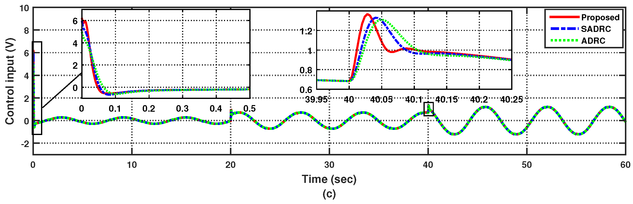
In this case, the tracking performance of the SBW system is examined under the nominal dynamics with time delays. For the purpose of conducting this case study, both the parametric uncertainties defined in (2) and the external disturbance specified in (5) have been set to zero. In addition, the input and output time lags illustrated in Figure 1 have been allotted values of sec and sec, correspondingly. Moreover, the aggregate of and is ensured to be smaller than the sampling time . Furthermore, as illustrated in Figure 5a, the reference angle of the front wheels has a sinusoidal pattern. In Figure 4a–d, the estimation errors for , , , and are illustrated, showcasing the exceptional estimation capability demonstrated by the proposed approach when it is contrasted with the methods of ADRC and SADRC. It can be observed that the estimation error of the proposed approach is narrower than that of the two alternative comparison techniques, whereas the rate of convergence for estimation in the proposed approach is higher. Furthermore, it is noteworthy that small peaking phenomenon arises within the estimated errors, primarily stemming from the high observer gains. Nevertheless, the observer gains cannot be set too low since it is also necessary to ensure a rapid tracking rate, minimal tracking error, and robust system performance. In Figure 5a–c, the graphs present the curves of the steering angle , the tracking error of , and the control input under the proposed control approach as well as the competing methods. In Figure 5a,b, it is apparent that the rate of convergence achieved through the proposed control technique surpasses that of ADRC and SADRC, while the tracking error in the proposed approach is diminished, as the effect of time lags is efficiently reduced in the proposed control strategy. Furthermore, Figure 5c demonstrates that the proposed control method exhibits a faster response in the control input compared to the other two comparison methods, whereas the maximum values of the control input among all three methods remain similar.
4.2. Case 2: Uncertain Steering for a Sinusoidal Reference Following the Input and Output Time Delay
Compared with Case 1, the parameter uncertainties stated in (2) are newly taken into account in Case 2. The transmission time delays are set to s and s, respectively. Hence, the combination of and is equal to the sampling time . In Figure 6a–d, the corresponding estimation errors of , , , and are presented. We can observe that the proposed control strategy continues to demonstrate superior estimation performance compared to those of the two comparison methods, exhibiting a swifter estimation convergence rate and smaller estimation errors. Furthermore, it is evident from Figure 7a–c that the tracking error of within the proposed control framework maintains a lower magnitude than that observed in the ADRC and SADRC methods, while the convergence speed of the tracking error and the responsiveness of the control input in the proposed control technique are enhanced.
4.3. Case 3: Uncertain Steering for a Sinusoidal Reference Following the Time-Varying Delays and External Disturbances
Compared with Case 2, not only the parameter uncertainties given in Equation (2) are taken into account but also the time-varying delays s and s and the external disturbance Nm. The simulation results of the steering angle , the tracking error of , and the control input for Case 3 are presented in Figure 8a–c. A comparison of Figure 8a–c reveals that the proposed control method continues to outperform the other two comparison methods. This indicates that the proposed control method effectively compensates for parameter uncertainties and external disturbance amidst time-varying input and output delays. In practical applications, if the front wheels track their reference slowly or with large tracking errors, it can lead to delayed or inaccurate path changes in the vehicle, particularly in dangerous traffic conditions. This situation poses a significant safety risk. As shown in Figure 5b, Figure 7b, and Figure 8b, and their corresponding Case 1, Case 2, and Case 3 analyses, the proposed control scheme offers improved driving safety in the SBW system compared with two existing control algorithms. This is achieved through swifter convergence rates and diminished tracking errors of the front wheels.
5. Conclusions
In an effort to enhance the performance of the steering-by-wire (SBW) system, this paper proposes a novel robust fast finite-time composite control algorithm. This algorithm is designed to precisely track the front wheel angles in response to the desired command from the hand wheel within a fast finite time, overcoming challenges posed by time delays and uncertainties. The proposed controller was examined across three distinct scenarios: nominal steering involving input and output time delays; uncertain steering entailing both uncertainties and transmission time delay; and the final scenario encompassing uncertainties, transmission time delay, and external disturbances. To verify the outperformance of our proposed method, simulations are conducted, and the results are compared with two benchmark control methods, namely, ADRC and SADRC. The simulation results indicate the superiority of the proposed controller over the two comparative methods. Lastly, the findings emphasize the effectiveness of the proposed control method in entirely addressing parameter uncertainties and external disturbances, even in challenging conditions characterized by time-varying input and output delays. Moreover, the discerned accelerated convergence rate of the front wheels’ tracking errors, coupled with the reduction in the tracking errors, provides compelling evidence that the proposed method enhances driving safety in the SBW system, even when facing various uncertainties. While we acknowledge the importance of experimental validation, we view this work as a foundational step. Future research will undoubtedly include experimental studies to bridge the gap between simulation and reality, ensuring the robustness and effectiveness of the proposed controller in actual automotive scenarios. Furthermore, to reduce noise measurement caused by the sensitivity of sensors, the noise-free FFTCC scheme will be studied.
Author Contributions
Conceptualization, K.R., Z.C. and Z.M.; methodology, K.R. and Z.C.; software, K.R.; validation, K.R., J.K., Y.Z., Z.C. and Z.M.; formal analysis, J.K. and Y.Z.; investigation, K.R., Z.C., J.K. and Y.Z.; resources, Z.C. and Z.M.; writing—original draft preparation, J.K., Y.Z. and K.R.; writing—review and editing, K.R., J.K., Y.Z., Z.C. and Z.M.; visualization, J.K, Y.Z., K.R., Z.C. and Z.M.; supervision, Z.C. and Z.M.; project administration, Z.C. All authors have read and agreed to the published version of the manuscript.
Funding
This work was supported in part by the Australian Research Council Discovery Project under Grant DP190101557.
Informed Consent Statement
Not applicable.
Data Availability Statement
The original contributions presented in the study are included in the article, further inquiries can be directed to the corresponding author.
Acknowledgments
Kamal Rsetam would like to thank the Republic of Iraq/Ministry of Higher Education and Scientific Research and the University of Baghdad/Al Khwarizmi College of Engineering for granting a Research Fellow.
Conflicts of Interest
The authors declare no conflict of interest.
References
- Chen, T.; Xu, X.; Chen, L.; Jiang, H.; Cai, Y.; Li, Y. Estimation of longitudinal force, lateral vehicle speed, and yaw rate for four-wheel independent driven electric vehicles. Mech. Syst. Signal Process. 2018, 101, 377–388. [Google Scholar] [CrossRef]
- Wang, R.; Hu, C.; Wang, Z.; Yan, F.; Chen, N. Integrated optimal dynamics control of 4WD4WS electric ground vehicle with tire-road frictional coefficient estimation. Mech. Syst. Signal Process. 2015, 60, 727–741. [Google Scholar] [CrossRef]
- Zhang, L.; Zhang, Z.; Wang, Z.; Deng, J.; Dorrell, D.G. Chassis coordinated control for full X-by-wire vehicles-A review. Chin. J. Mech. Eng. 2021, 34, 1–25. [Google Scholar] [CrossRef]
- Wang, Z.; Li, Y.; Kaku, C.; Zheng, H. Trajectory Tracking Control of Intelligent X-by-Wire Vehicles. World Electr. Veh. J. 2022, 13, 205. [Google Scholar] [CrossRef]
- Chen, T.; Cai, Y.; Chen, L.; Xu, X.; Sun, X. Trajectory tracking control of steer-by-wire autonomous ground vehicle considering the complete failure of vehicle steering motor. Simul. Model. Pract. Theory 2021, 109, 102235. [Google Scholar] [CrossRef]
- Huang, C.; Naghdy, F.; Du, H. Sliding mode predictive tracking control for uncertain steer-by-wire system. Control Eng. Pract. 2019, 85, 194–205. [Google Scholar] [CrossRef]
- Kong, H.; Liu, T.; Fang, Y.; Yan, J. Robust steering control for a steer-by-wire automated guided vehicle via fixed-time adaptive recursive sliding mode. Trans. Inst. Meas. Control 2023, 45, 2590–2601. [Google Scholar] [CrossRef]
- Pietruch, M.; Wetula, A.; Młyniec, A. Influence of the Accuracy and CAN Frame Period of the Steering Wheel Angle Sensor (SAS) on the Trajectory of a Steer-by-Wire-Equipped Car. IEEE Access 2022, 10, 106110–106116. [Google Scholar] [CrossRef]
- Shao, W.; Liang, X.; Fang, T.; Zhao, L.; Hu, Y. Active steering stability control of steer-by-wire vehicles based on variable horizon-robust model predictive control. J. Braz. Soc. Mech. Sci. Eng. 2023, 45, 410. [Google Scholar] [CrossRef]
- Sun, Z.; Zheng, J.; Man, Z.; Wang, H. Robust control of a vehicle steer-by-wire system using adaptive sliding mode. IEEE Trans. Ind. Electron. 2015, 63, 2251–2262. [Google Scholar] [CrossRef]
- Wang, H.; Man, Z.; Kong, H.; Zhao, Y.; Yu, M.; Cao, Z.; Zheng, J.; Do, M.T. Design and implementation of adaptive terminal sliding-mode control on a steer-by-wire equipped road vehicle. IEee Trans. Ind. Electron. 2016, 63, 5774–5785. [Google Scholar] [CrossRef]
- Sun, Z.; Zheng, J.; Wang, H.; Man, Z. Adaptive fast non-singular terminal sliding mode control for a vehicle steer-by-wire system. IET Control Theory and Appl. 2017, 11, 1245–1254. [Google Scholar] [CrossRef]
- Sun, Z.; Zheng, J.; Man, Z.; Fu, M.; Lu, R. Nested adaptive super-twisting sliding mode control design for a vehicle steer-by-wire system. Mech. Syst. Signal Process. 2019, 122, 658–672. [Google Scholar] [CrossRef]
- Shi, Q.; He, S.; Wang, H.; Stojanovic, V.; Shi, K.; Lv, W. Extended state observer based fractional order sliding mode control for steer-by-wire systems. IET Control Theory and Appl. 2023; early view. [Google Scholar]
- Liang, X.; Zhao, L.; Wang, Q.; Chen, W.; Xia, G.; Hu, J.; Jiang, P. A novel steering-by-wire system with road sense adaptive friction compensation. Mech. Syst. Signal Process. 2022, 169, 108741. [Google Scholar] [CrossRef]
- Shukla, H.; Roy, S.; Gupta, S. Robust adaptive control of steer-by-wire systems under unknown state-dependent uncertainties. Int. J. Adapt. Control Signal Process. 2022, 36, 198–208. [Google Scholar] [CrossRef]
- Ye, M.; Wang, H. Robust adaptive integral terminal sliding mode control for steer-by-wire systems based on extreme learning machine. Comput. Electr. Eng. 2020, 86, 106756. [Google Scholar] [CrossRef]
- Zhang, J.; Wang, H.; Ma, M.; Yu, M.; Yazdani, A.; Chen, L. Active front steering-based electronic stability control for steer-by-wire vehicles via terminal sliding mode and extreme learning machine. IEEE Trans. Veh. Technol. 2020, 69, 14713–14726. [Google Scholar] [CrossRef]
- Zhao, J.; Yang, K.; Cao, Y.; Liang, Z.; Li, W.; Xie, Z.; Wong, P.K. Observer-Based Discrete-Time Cascaded Control for Lateral Stabilization of Steer-by-Wire Vehicles With Uncertainties and Disturbances. IEEE Trans. Circuits Syst. Regul. Pap. 2023. [Google Scholar] [CrossRef]
- Wang, Y.; Liu, Y.; Wang, Y.; Chai, T. Neural output feedback control of automobile steer-by-wire system with predefined performance and composite learning. IEEE Trans. Veh. Technol. 2023, 72, 5906–5921. [Google Scholar] [CrossRef]
- Li, Z.; Jiao, X.; Zhang, T. Robust H∞ Output Feedback Trajectory Tracking Control for Steer-by-Wire Four-Wheel Independent Actuated Electric Vehicles. World Electr. Veh. J. 2023, 14, 147. [Google Scholar] [CrossRef]
- Shah, M.B.N.; Husain, A.R.; Aysan, H.; Punnekkat, S.; Dobrin, R.; Bender, F.A. Error handling algorithm and probabilistic analysis under fault for CAN-based steer-by-wire system. IEEE Transactions Ind. Inform. 2016, 12, 1017–1034. [Google Scholar] [CrossRef]
- Lu, Y.; Liang, J.; Wang, F.; Yin, G.; Pi, D.; Feng, J.; Liu, H. An active front steering system design considering the CAN network delay. IEEE Transactions Transp. Electrif. 2023, 9, 5244–5256. [Google Scholar] [CrossRef]
- Ye, Q.; Wang, R.; Cai, Y.; Chadli, M. The stability and accuracy analysis of automatic steering system with time delay. ISA Trans. 2020, 104, 278–286. [Google Scholar] [CrossRef] [PubMed]
- Yang, Y.; Yan, Y.; Xu, X. Fractional order adaptive fast super-twisting sliding mode control for steer-by-wire vehicles with time-delay estimation. Electronics 2021, 10, 2424. [Google Scholar] [CrossRef]
- Zhang, B.; Zhao, W.; Wang, C.; Lian, Y. Layered Time-delay Robust Control Strategy for Yaw Stability of SBW Vehicles. IEEE Trans. Intell. Veh. 2023, 8, 1–11. [Google Scholar] [CrossRef]
- Yih, P.; Gerdes, J.C. Modification of vehicle handling characteristics via steer-by-wire. IEEE Trans. Control Syst. Technol. 2005, 13, 965–976. [Google Scholar] [CrossRef]
- Rajamani, R. Vehicle Dynamics and Control; Springer: New York, NY, USA, 2012. [Google Scholar]
- Wang, H.; Kong, H.; Man, Z.; Tuan, D.; Cao, Z.; Shen, W. Sliding mode control for steer-by-wire systems with AC motors in road vehicles. IEEE Trans. Ind. Electron. 2013, 61, 1596–1611. [Google Scholar] [CrossRef]
- Baviskar, A.; Wagner, J.R.; Dawson, D.M.; Braganza, D.; Setlur, P. An adjustable steer-by-wire haptic-interface tracking controller for ground vehicles. IEEE Trans. Veh. Technol. 2008, 58, 546–554. [Google Scholar] [CrossRef]
- Wu, Q.; Yu, L.; Wang, Y.W.; Zhang, W.A. LESO-based position synchronization control for networked multi-axis servo systems with time-varying delay. IEEE/CAA J. Autom. Sin. 2020, 7, 1116–1123. [Google Scholar] [CrossRef]
- Moulay, E.; Perruquetti, W. Finite time stability conditions for non-autonomous continuous systems. Int. J. Control 2008, 81, 797–803. [Google Scholar] [CrossRef]
- Bhat, S.P.; Bernstein, D.S. Finite-time stability of continuous autonomous systems. SIAM J. Control Optim. 2000, 38, 751–766. [Google Scholar] [CrossRef]
- Bacciotti, A.; Rosier, L. Liapunov Functions and Stability in Control Theory; Springer: Berlin/Heidelberg, Germany, 2005. [Google Scholar]
- Li, J.; Qian, C.; Ding, S. Global finite-time stabilisation by output feedback for a class of uncertain nonlinear systems. International Journal of Control. Int. J. Control 2010, 83, 2241–2252. [Google Scholar] [CrossRef]
- Zhu, W.; Du, H.; Li, S.; Yu, X. Design of output-based finite-time convergent composite controller for a class of perturbed second-order nonlinear systems. IEEE Trans. Syst. Man, Cybern. Syst. 2020, 51, 6768–6778. [Google Scholar] [CrossRef]
- Hong, Y.; Huang, J.; Xu, Y. On an output feedback finite-time stabilization problem. IEEE Trans. Autom. Control 2001, 46, 305–309. [Google Scholar] [CrossRef]
- Orlov, Y.; Aoustin, Y.; Chevallereau, C. Finite time stabilization of a perturbed double integrator—Part I: Continuous sliding mode-based output feedback synthesis. IEEE Trans. Autom. Control 2010, 56, 614–618. [Google Scholar] [CrossRef]
- Levant, A. Higher-order sliding modes, differentiation and output-feedback control. Int. J. Control 2003, 76, 924–941. [Google Scholar] [CrossRef]
- Li, G.; Wang, X.; Li, S. Finite-time output consensus of higher-order multiagent systems with mismatched disturbances and unknown state elements. IEEE Trans. Syst. Man, Cybern. Syst. 2017, 49, 2571–2581. [Google Scholar] [CrossRef]
- Qian, C.; Lin, W. Output feedback control of a class of nonlinear systems: A nonseparation principle paradigm. IEEE Trans. Autom. Control 2002, 47, 1710–1715. [Google Scholar] [CrossRef]
- Du, H.; Qian, C.; Yang, S.; Li, S. Recursive design of finite-time convergent observers for a class of time-varying nonlinear systems. Automatica 2013, 49, 601–609. [Google Scholar] [CrossRef]
- Han, J. From PID to Active Disturbance Rejection Control. IEEE Trans. Ind. Electron. 2009, 56, 900–906. [Google Scholar] [CrossRef]
Figure 1.
Architecture of SBW system with time delays of the transmission channel.
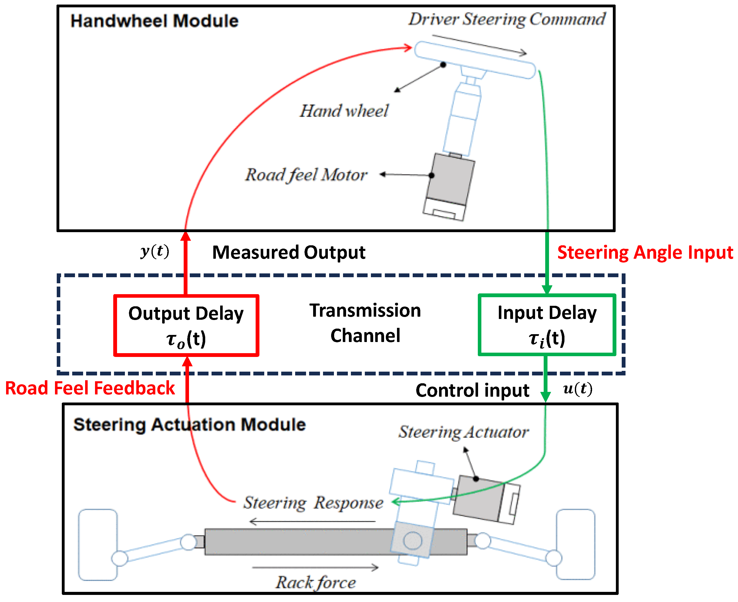
Figure 2.
Configuration of the proposed composite tracking controller for the SBW system.
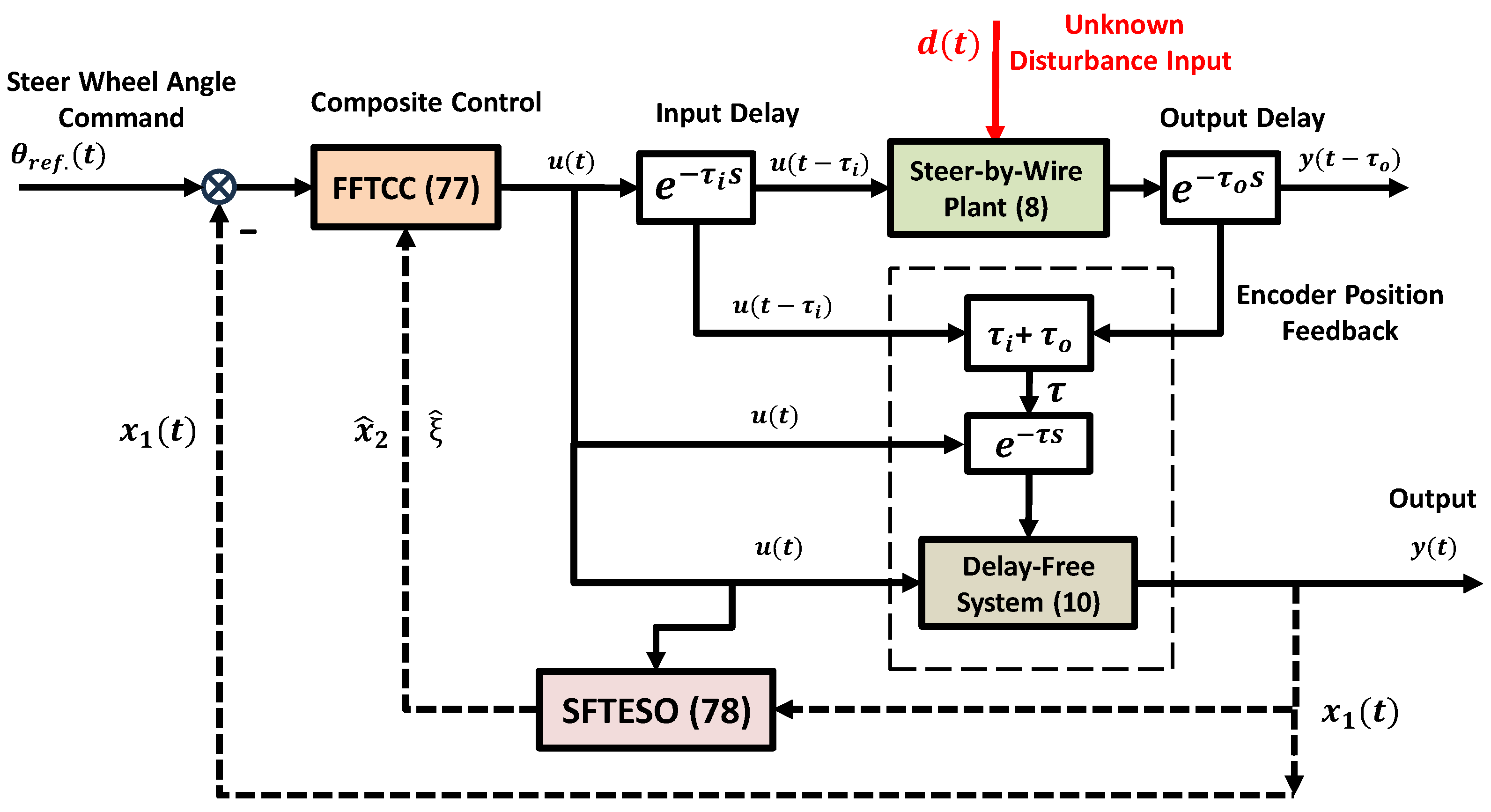
Figure 3.
Flow chart of applying the proposed control method to the SBW system.
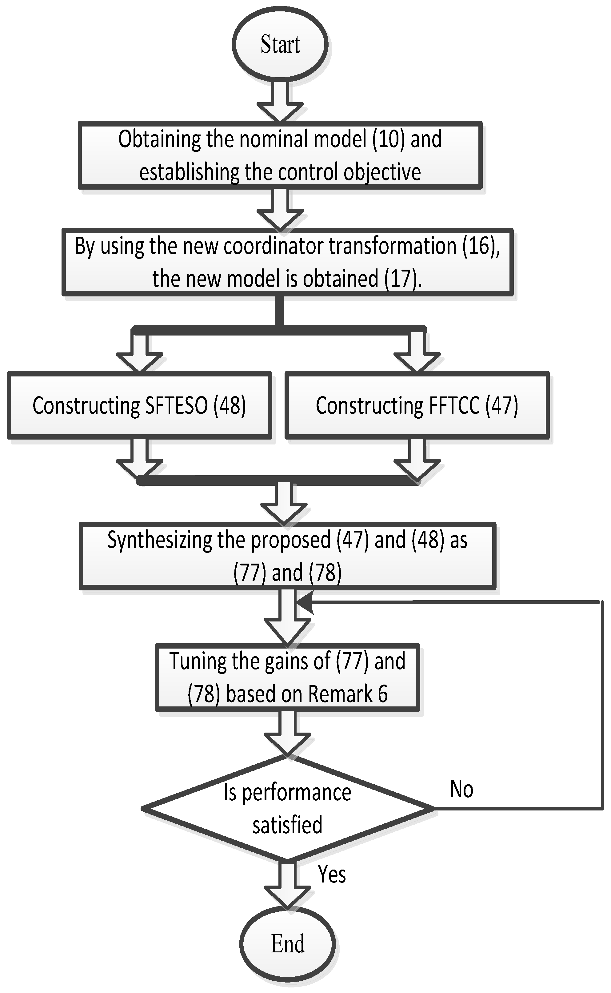
Figure 4.
Estimation error responses under (Case 1). (a) Position estimation error. (b) Velocity estimation error. (c) Overall disturbance estimation error . (d) Delayed input estimation error.
Figure 4.
Estimation error responses under (Case 1). (a) Position estimation error. (b) Velocity estimation error. (c) Overall disturbance estimation error . (d) Delayed input estimation error.
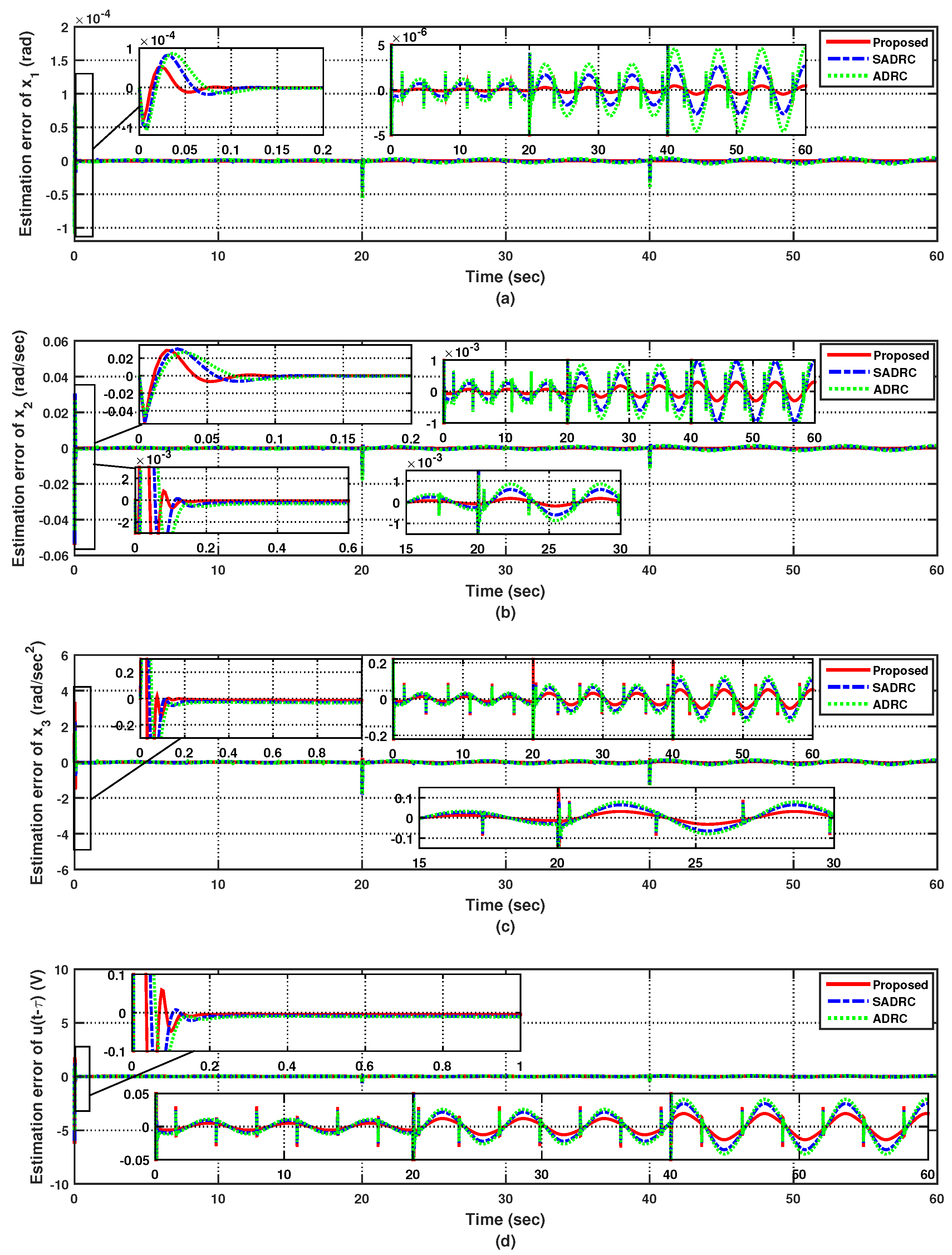
Figure 5.
Tracking responses for the nominal system under the input time delay s and the output time delay s (Case 1). (a) Steering angle. (b) Tracking error. (c) Control input.
Figure 5.
Tracking responses for the nominal system under the input time delay s and the output time delay s (Case 1). (a) Steering angle. (b) Tracking error. (c) Control input.
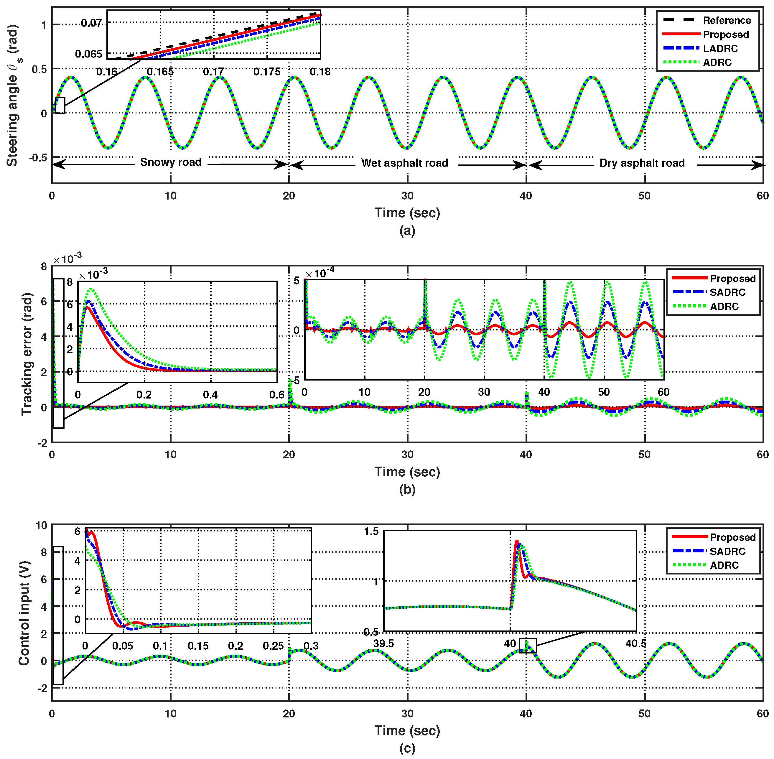
Figure 6.
Estimation error responses under (Case 2). (a) Position estimation error. (b) Velocity estimation error. (c) Overall disturbance estimation error . (d) Delayed input estimation error.
Figure 6.
Estimation error responses under (Case 2). (a) Position estimation error. (b) Velocity estimation error. (c) Overall disturbance estimation error . (d) Delayed input estimation error.
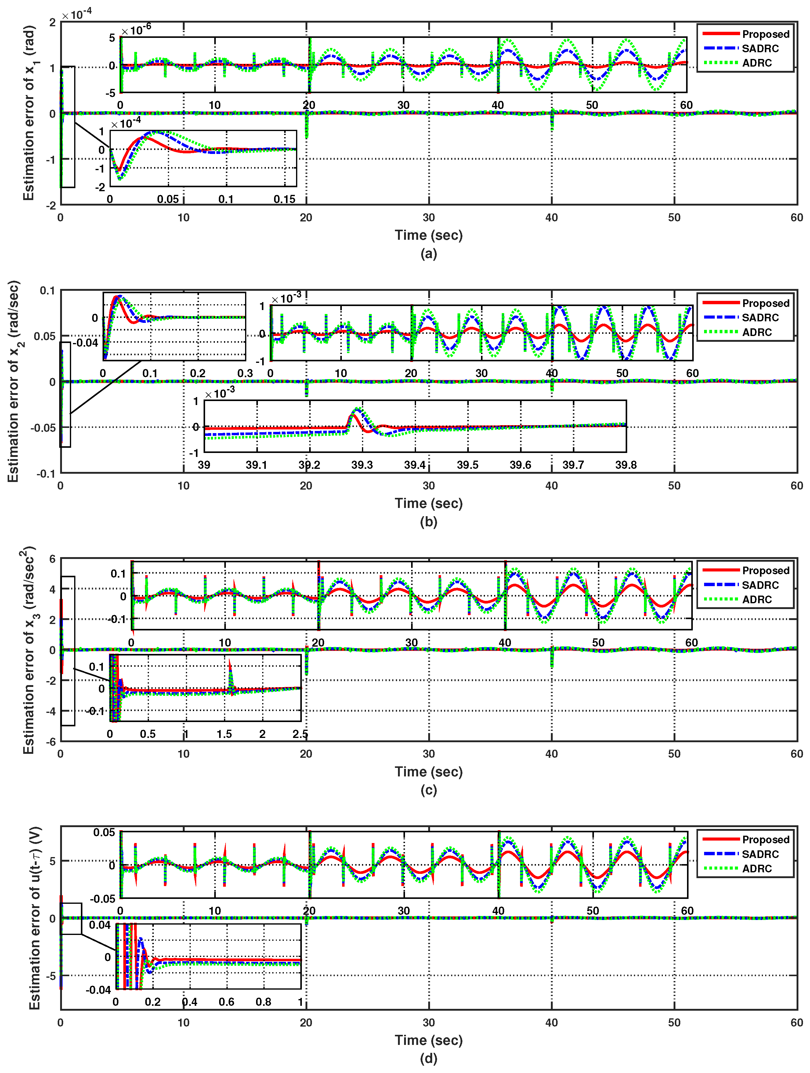
Figure 7.
Tracking responses for the uncertain system under the input time delay s and the output time delay s (Case 2). (a) Steering angle. (b) Tracking error. (c) Control input.
Figure 7.
Tracking responses for the uncertain system under the input time delay s and the output time delay s (Case 2). (a) Steering angle. (b) Tracking error. (c) Control input.
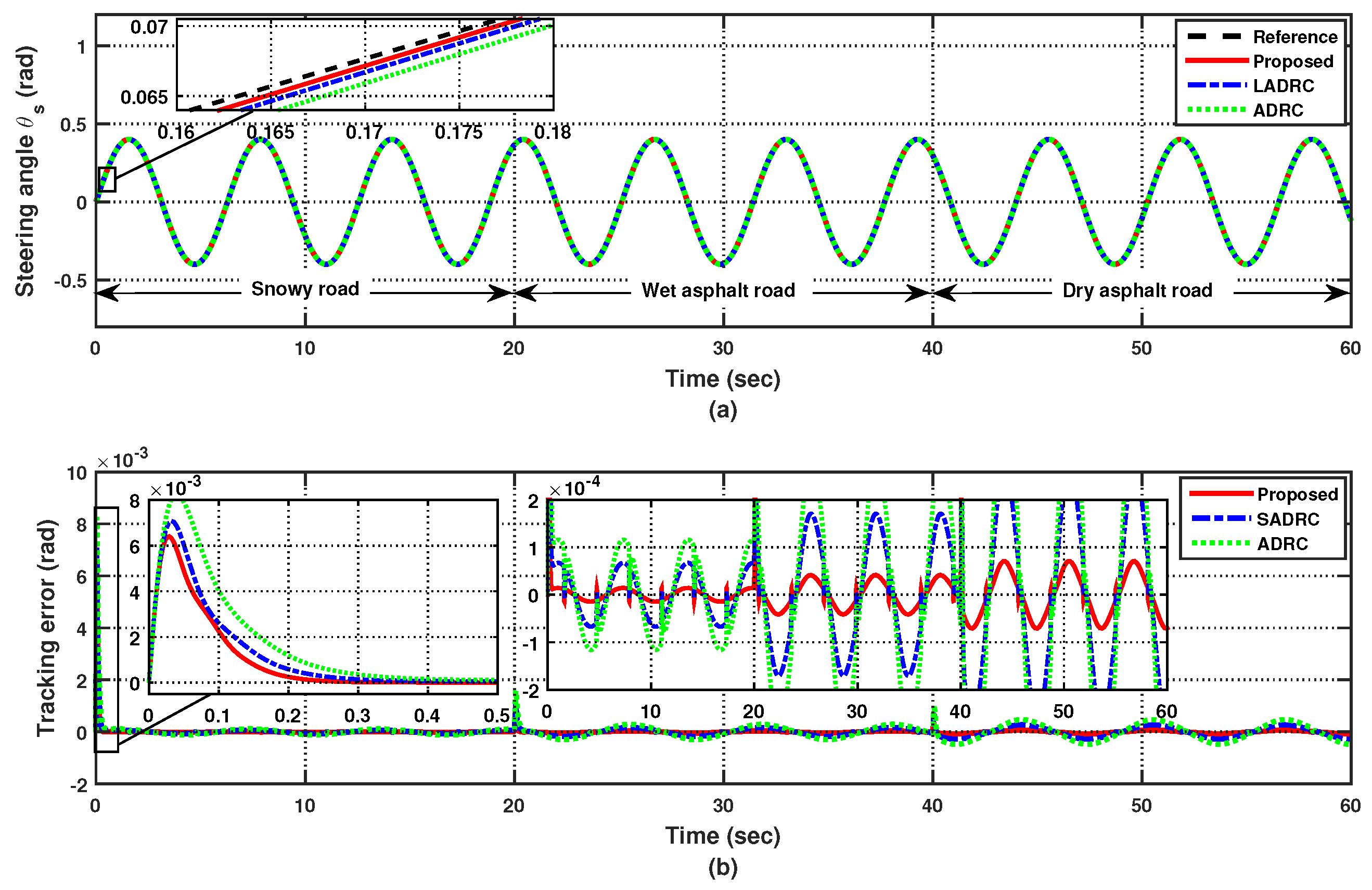
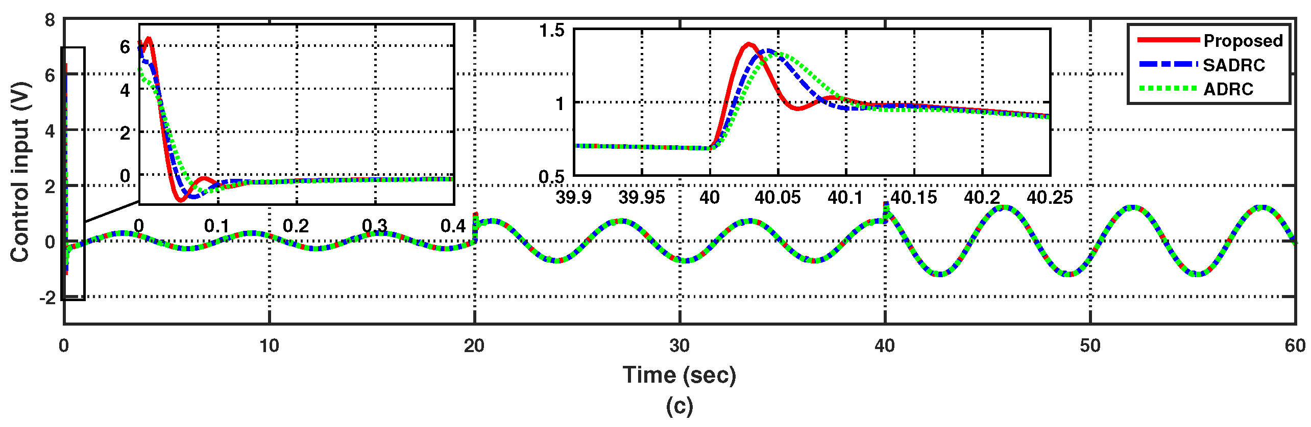
Figure 8.
Tracking responses for the uncertain system under the time-varying input delay s, the time-varying output delay s, and the external disturbance Nm (Case 3). (a) Steering angle. (b) Tracking error. (c) Control input.
Figure 8.
Tracking responses for the uncertain system under the time-varying input delay s, the time-varying output delay s, and the external disturbance Nm (Case 3). (a) Steering angle. (b) Tracking error. (c) Control input.


Table 1.
Nominal parameters of SBW system.
| Symbols | Descriptions | Values | Units |
|---|---|---|---|
| Equivalent inertial moment of the SBW system | 85.5 | kg m2 | |
| Equivalent viscous damping friction of the SBW system | 218.8 | N ms/rad | |
| Coulomb friction constant | 4.2 | N m | |
| Scale factor to account for transmitting from the linear motion of the rack to the steering angle of front wheels | 6.0 | - | |
| Gear ratio between the pinion and rack system | 3.0 | - | |
| Gear ratio of the gear head | 8.5 | - | |
| Scale factor accounting for converting from the input voltage of steering motor to the output torque of steering motor | 1.8 | - |
Disclaimer/Publisher’s Note: The statements, opinions and data contained in all publications are solely those of the individual author(s) and contributor(s) and not of MDPI and/or the editor(s). MDPI and/or the editor(s) disclaim responsibility for any injury to people or property resulting from any ideas, methods, instructions or products referred to in the content. |
© 2024 by the authors. Licensee MDPI, Basel, Switzerland. This article is an open access article distributed under the terms and conditions of the Creative Commons Attribution (CC BY) license (https://creativecommons.org/licenses/by/4.0/).
Share and Cite
MDPI and ACS Style
Rsetam, K.; Khawwaf, J.; Zheng, Y.; Cao, Z.; Man, Z. Fast Finite-Time Composite Controller for Vehicle Steer-by-Wire Systems with Communication Delays. World Electr. Veh. J. 2024, 15, 132. https://doi.org/10.3390/wevj15040132
AMA Style
Rsetam K, Khawwaf J, Zheng Y, Cao Z, Man Z. Fast Finite-Time Composite Controller for Vehicle Steer-by-Wire Systems with Communication Delays. World Electric Vehicle Journal. 2024; 15(4):132. https://doi.org/10.3390/wevj15040132
Chicago/Turabian StyleRsetam, Kamal, Jasim Khawwaf, Yusai Zheng, Zhenwei Cao, and Zhihong Man. 2024. "Fast Finite-Time Composite Controller for Vehicle Steer-by-Wire Systems with Communication Delays" World Electric Vehicle Journal 15, no. 4: 132. https://doi.org/10.3390/wevj15040132