

Optimal Allocation of Fast Charging Stations on Real Power Transmission Network with Penetration of Renewable Energy Plant

Department of Electrical Engineering, College of Engineering, Jouf University, Sakaka 72388, Saudi Arabia
*
Author to whom correspondence should be addressed.
World Electr. Veh. J. 2024, 15(4), 172; https://doi.org/10.3390/wevj15040172
Submission received: 23 March 2024
/
Revised: 11 April 2024
/
Accepted: 12 April 2024
/
Published: 20 April 2024
(This article belongs to the Special Issue Sustainable EV Rapid Charging, Challenges, and Development)
Abstract
:Because of their stochastic nature, the high penetration of electric vehicles (EVs) places demands on the power system that may strain network reliability. Along with increasing network voltage deviations, this can also lower the quality of the power provided. By placing EV fast charging stations (FCSs) in strategic grid locations, this issue can be resolved. Thus, this work suggests a new methodology incorporating an effective and straightforward Red-Tailed Hawk Algorithm (RTH) to identify the optimal locations and capacities for FCSs in a real Aljouf Transmission Network located in northern Saudi Arabia. Using a fitness function, this work’s objective is to minimize voltage violations over a 24 h period. The merits of the suggested RTH are its high convergence rate and ability to eschew local solutions. The results obtained via the suggested RTH are contrasted with those of other approaches such as the use of a Kepler optimization algorithm (KOA), gold rush optimizer (GRO), grey wolf optimizer (GWO), and spider wasp optimizer (SWO). Annual substation demand, solar irradiance, and photovoltaic (PV) temperature datasets are utilized in this study to describe the demand as well as the generation profiles in the proposed real network. A principal component analysis (PCA) is employed to reduce the complexity of each dataset and to prepare them for the k-means algorithm. Then, k-means clustering is used to partition each dataset into k distinct clusters evaluated using internal and external validity indices. The values of these indices are weighted to select the best number of clusters. Moreover, a Monte Carlo simulation (MCS) is applied to probabilistically determine the daily profile of each data set. According to the obtained results, the proposed RTH outperformed the others, achieving the lowest fitness value of 0.134346 pu, while the GRO came in second place with a voltage deviation of 0.135646 pu. Conversely, the KOA was the worst method, achieving a fitness value of 0.148358 pu. The outcomes attained validate the suggested approach’s competency in integrating FCSs into a real transmission grid by selecting their best locations and sizes.
1. Introduction
Fossil fuel consumption has increased dramatically recently, particularly in the transportation and electricity generation industries. Due to their greenhouse gas emissions and contribution to global warming, these sources exacerbate environmental pollution [1]. In order to lessen pollution, many nations are looking to switch from gasoline-powered cars to clean energy vehicles known as electric vehicles (EVs) [2]. EVs are more cost-effective and environmentally friendly than gasoline-powered vehicles. Because of their sophisticated batteries and power electronics, EVs can operate as controlled loads on a grid. One of the biggest obstacles to integrating EVs into a power system is the potential for overload-related transmission line thermal constraints to be violated, which could result in voltage drops in some sensitive buses in the network. Additionally, the distribution network operator faces difficulties due to uncertainties surrounding these vehicles. These uncertainties stem from factors like daily energy consumption, time rounding, EV battery capacity, and EV driving range [3]. EVs are typically charged at public charging stations using fast charging stations (FCSs), which demand high power from the grid to shorten the time needed to meet the battery’s state-of-charge (SOC) requirements. However, the distribution network is negatively impacted by the high power demand of these stations, increasing voltage deviations and power losses. However, renewable energy sources (RESs) can be installed to supply excess loads during peak hours and lessen the demand on the grid. To reduce the negative effects that come with FCSs, it is imperative to determine the best locations for them within the distribution network. Numerous documented methods have been used to determine optimal FCS sizes and locations.
To reduce active and reactive power losses in the system as well as the investment cost, a workable methodology for choosing optimal locations of FCSs in distribution networks was proposed [4]. The methodology mitigated the managed network’s active power loss from 1015.38 kW to 830.58 kW. One other option for reducing the impact of these stations is to integrate photovoltaic systems. A bi-level optimization framework for improving the performance of distribution and transmission networks was developed in [5]. In order to minimize power purchase costs and maximize the penetration of renewable sources and EV charging stations, the approach optimized the operations of both renewable and nonrenewable sources in the presence of EV charging stations. Using a clustering-based heuristic, the best locations for EV charging stations throughout the French national network were found, resulting in an optimized trip time for lengthy trips [6]. The deployment of PV-powered EV fast charging stations and energy storage systems in distribution and transportation networks was optimized by the authors of [7] using particle swarm optimization (PSO) and a hybrid fuzzy–satisfaction technique. They concluded that the installation of both solar PVs and an energy storage system with optimal locations for FCSs improved the network’s mean voltage deviation reliability index by 18.79% compared to the base scenario. To find and seize EV charging stations in a transportation network, a bi-level mixed-integral programming approach has been created [8]. This framework’s primary goal is to decrease the overall traffic time and investment costs. The optimal locations and capacities of distributed generation (DG) and charging stations for electric vehicles (EVs) in balanced radial distribution networks have been assessed using a bat optimization technique [9]. The optimal locations and sizes for renewable energy sources and EV fast charging stations in balanced distribution networks are determined using a red kite optimizer, as described in [10]. The presented approach succeeded in mitigating power losses for 33-bus and 69-bus networks by 58.24% and 68.39%, respectively. The goal was to lessen the network’s daily power losses and voltage violations. In a coupled electrical power distribution and transportation network, the authors of [11] presented a multi-objective PSO with a constriction factor to determine the best locations and sizes of fast charging stations along intra-city corridors. To improve EV drivers’ charging decisions, a multi-agent actor–critic algorithm combined with embedded graph attention networks has been presented [12]. This algorithm used graph attention networks to take advantage of the interfaces between agents’ observations. A thorough analysis of the architecture and concepts for EV fast charging stations, along with their practical applications, was carried out in [13]. Furthermore, a number of optimization techniques used in the location and acquisition of FCSs have been considered. Using real-world data, the authors of [14] presented a customized sub-gradient method-based data-driven framework to evaluate the profitability of FCSs. Under ideal circumstances, the savings could reach 34.0%, and when user behavior and battery degradation were taken into consideration, the savings could reach 22.6%. A grey wolf optimizer (GWO) was used to arrange the grid charging of EVS ecosystems in order to maximize profits while adhering to operating constraints [15]. Extremely quick charging stations and energy storage systems for EVs were distributed throughout a grid in [16] using a Markov decision process solved via a deep deterministic policy gradient with constraints. To assess the best locations for DGs and EV charging stations within the distribution network that minimize active power loss while enhancing the voltage profile and voltage stability index, a methodology that incorporates a transient search optimizer has been presented [17]. A demand and supply analysis was used to determine the best locations for EV infrastructure on a highway network, considering the psychological aspects of driving [18]. With the help of dynamic real data, the authors of [19] integrated FCSs into Beijing’s third ring in order to optimize the power grid, traffic conditions, vehicles, and operators. In order to assess optimal locations for EV charging stations within distribution networks and to manage the charge/discharge schedules of these stations, a multi-objective PSO utilizing a Monte Carlo simulation was presented [20]. A reduction in power loss, the minimization of power purchased from the network, the mitigation of voltage deviation, and enhanced reliability were the primary goals. A bi-level programming technique was presented in [21] to achieve the best possible coordination between DGs and EV charging stations placed in distribution networks, maximizing profit for the power supply company. PSO was used by the authors of [22] to integrate EVs into the National University of Sciences and Technology’s actual distribution network in Pakistan while minimizing transformer loading, installation costs, and network losses. The EV charging infrastructure cost was reduced by 75% and the network losses were mitigated by 82% using the presented approach. The locations of EV charging stations in a distribution network overlayed with a traffic network have been optimized using differential evolution and Harris hawks optimizers to minimize energy loss, voltage violation, and land cost [23]. Using a surrogate assisted optimizer, the issue of integrating EV fast charging stations into a real flexible bus service in Luxembourg was resolved in [24]. Numerous methods for incorporating EV charging stations into distribution networks and analyzing how EVs affect cost, environmental factors, and network operation have been examined [25]. In order to incorporate electric vehicle charging stations into the Guwahati distribution network in India, a hybrid methodology combining a chicken swarm optimizer and a teaching–learning-based optimizer has been developed [26]. The goals were to reduce operating costs, maximize reliability, improve voltage stability, and minimize power loss. In order to minimize travel time, the locations of charging stations along a road network were chosen using a multi-commodity flow problem approach [27]. To mitigate the effect of fast charging on the grid, an integrated solar PV generation system and charging station were included in an energy management strategy via optimal power flow [28]. Using a multi-objective GWO and a fuzzy satisfaction-based decision-making approach, the distribution network’s power loss and voltage violation were minimized, while the amount of EV flow in the transportation network was maximized [29]. This is how the EV fast charging stations were distributed in relation to the transportation system. An improved PSO and Voronoi diagrams were used to determine the best locations and sizes for FCSs within a distribution network [30]. In [31], the optimal locations and capacities of fast charging stations for plug-in electric vehicles were determined by a mixed integer linear programming model that took traffic effects into account. GAMS software was employed by the authors to resolve the issue. A hybrid strategy that integrates EV charging stations and capacitors into a distribution network using a quantum neural network and a Eurasian oystercatcher optimizer is presented in [32]. The goal was to increase network dependability while reducing active power loss. A genetic algorithm was used in [33] to determine the locations of EV charging stations in order to minimize the operating costs of a distribution network installed in Ireland. To optimize the placement of EV charging stations and capacitors in a grid so as to minimize overall loss, a refined version of the dragonfly optimizer was developed [34]. In order to reduce the costs associated with system construction, operation, maintenance, travel, and charging station power loss, the authors of [35] employed binary PSO to determine the capacity and location of FCSs in distribution networks. To maximize long-distance trip completions, charging stations were strategically placed in [36] using data from long-distance travel in the United States. In order to reduce network energy loss, voltage fluctuations, and costs associated with investment, operation, and maintenance, solar DGs, fast charging stations, and battery storage systems have been integrated into the distribution network in locations chosen by a Harris hawks optimizer and GWO [37]. A survey of various strategies for strategically placing electric vehicle charging stations can be found in [38]. Voltage restoration in a real railway network considering the behavior of the charging station installed in it was investigated in [39].
The slow convergence rate of some approaches used and the decrease in local optimal solutions account for the accuracy deficit of many reported methods.
The following contributions were made by the authors in order to address all of these shortcomings in the methods that were reported:
- A novel approach that incorporates the effective and straightforward Red-Tailed Hawk Algorithm (RTH) is proposed to identify optimal locations and capacities for FCSs in a real transmission network containing a PV plant.
- PV generation and demand profiles are developed using a principal component analysis and k-means clustering and estimated probabilistically based on a Monte Carlo simulation.
- The objective of a fitness function that is taken into consideration is to lower the network voltage deviation.
- A comparison is made with the KOA, GRO, GWO, and SWO.
- The outcomes attained validate the suggested approach’s competency.
The outline of the paper is as follows: Section 2 describes the electric vehicle model. The suggested optimization formula is addressed in Section 3. Section 4 presents the Red-Tailed Hawk Algorithm, and Section 5 provides the suggested approach that incorporates the RTH. Section 6 explains the probabilistic load modeling, Section 7 provides an explanation of the results and discussions, and Section 8 provides conclusions.
2. Electric Vehicle Model
Three factors need to be considered in order to model EVs: the anticipated daily mileage, the energy used per mile, and the amount of time spent waiting in the station. A lognormal distribution can be used to simulate the first one [40]; one can calculate the probability density function for the lognormal distribution as
where is a randomly generated number with zero mean and one variance; and denote parameters of scaling and location, computed as
where and stand for the mean and standard deviation, which are calculated using historical data. The following is an expression for the anticipated daily mileage:
where the lognormal probability distribution’s parameters are and ; the random variables and , which are in the interval [0, 1], have a normal distribution. Using the standard deviation () and mean () of the EV mileage statistical data, and can be computed as
The energy consumed per mile, which can be calculated as in [41], is the second crucial parameter that needs to be considered when modeling an EV; it can be expressed as follows:
where denotes the energy supplied by the battery, and and are coefficients of the EV model. When the battery is fully charged, the EV can reach its maximum mileage, as follows:
where denotes the capacity of the battery. The following formula can be used to calculate the charging demand:
The following formula can be used to determine the amount of time spent waiting in the station using a Gaussian distribution [42]:
where the times of departure, arrival, and charging are indicated by , , and , respectively, and and denote the standard deviations of the EV’s departure and arrival from the station, while and are the corresponding means. The random variables and have zero mean and one variance.
The following formula can be used to determine the EV battery’s necessary state of charge [42]:
where denotes the initial SOC of the battery, while is the rate of battery charging.
3. The Proposed Optimization Formula
Finding the optimal places and capacities for EV charging stations is approached as an optimization problem. The fitness function under consideration minimizes network voltage violations, and the constraints include generation boundaries, a supply and demand balance, bus voltage boundaries, thermal limitations, and EV-specific restrictions.
3.1. Problem Fitness Function
The integration of EV charging stations into a grid results in increased generation and an enhanced network bus voltage; therefore, mitigating the network’s daily voltage fluctuation is considered the target in this work, and it can be expressed as follows:
where the voltage at bus i during hour t is represented by and the number of network buses is indicated by .
3.2. Problem Constraints
Generation boundaries, the supply and demand balance, bus voltage boundaries, thermal limitations, and EV-specific restrictions are the problem constraints considered in this work, and they are explained below.
- A.
- Generation boundaries:
The system under consideration in this work is the real Aljouf Transmission Network located in northern Saudi Arabia. It contains a 300 MW photovoltaic (PV) plant in Sakaka which is a renewable energy plant. The production of such a plant should adhere to the following regulations:
where denotes the power generated by the PV plant at hour t, where the plant’s minimum and maximum generations are denoted, respectively, by and .
- B.
- Supply and demand balance:
A load flow analysis provides this constraint: the power supplied at each bus must equal the combined demand power and the branch power losses connected to it. These can be expressed as follows:
where and represent the generated and demanded active powers at bus i during hour t, respectively, denotes the power charged to the EV at bus i during hour t, and represent the generated and demanded reactive powers at bus i during hour t, respectively, and and denote the admittance magnitude of the branch between buses i and j and the angle between them, respectively.
- C.
- Bus voltage boundaries:
The bus voltage should be maintained within its typical ranges while integrating the charging station as follows:
where the terms and represent the respective values.
- D.
- Thermal limitations:
When the EV charging station is integrated into the grid, the power flow through the transmission lines increases, raising the temperature of the lines. However, the power flow cannot go beyond the permitted range, which is expressed as follows:
where represents the ith line flow during hour t and indicates the highest flow that is permitted in line i.
- E.
- EV-specific restrictions:
The EV’s power needs should fall between the following and values:
where indicates the EV’s output power at bus i during hour t and the minimum and maximum power values needed by the EV are denoted by and , respectively.
4. Red-Tailed Hawk Algorithm (RTH)
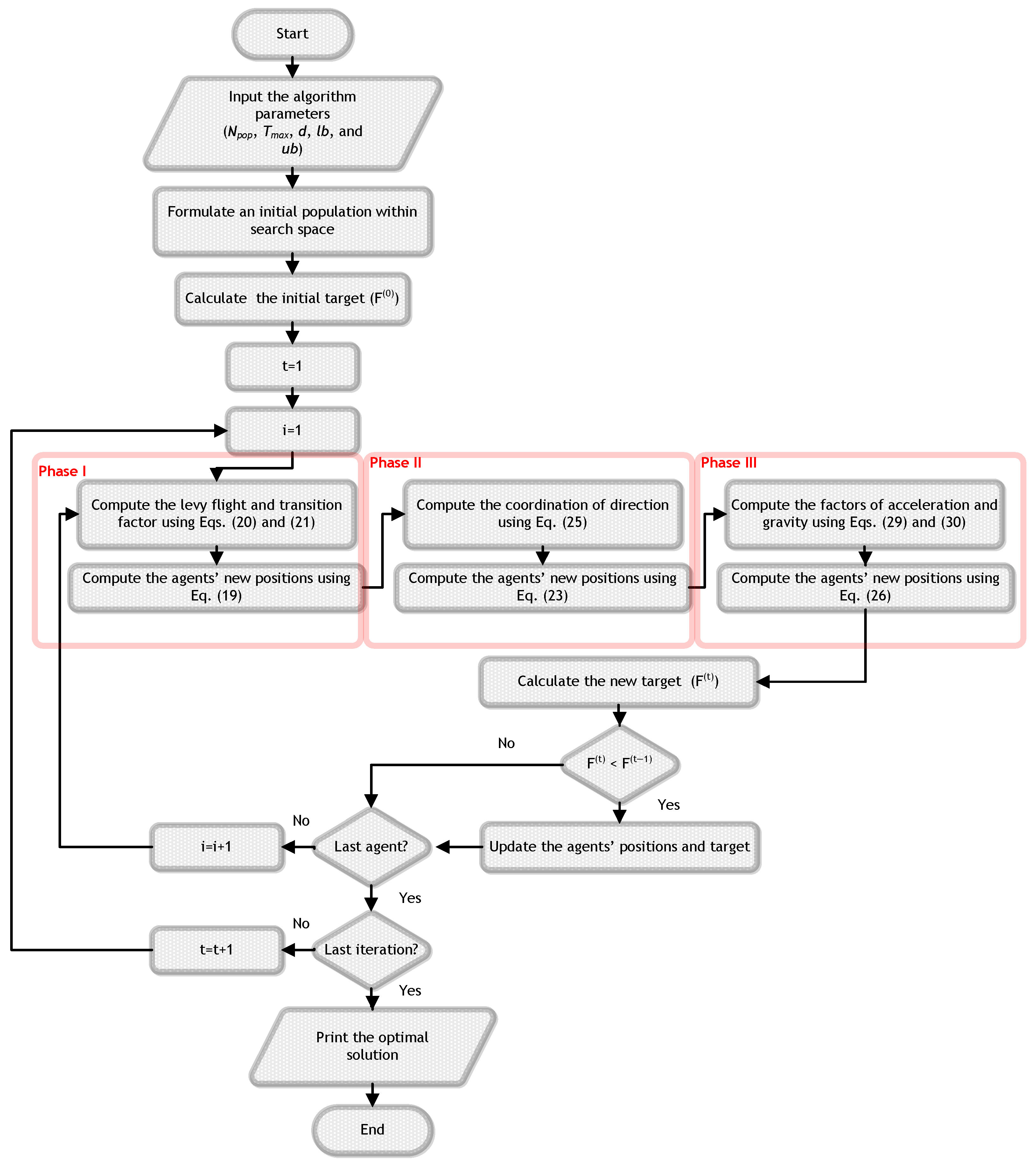
A red-tailed hawk hunting was the source of inspiration for Ferahtia et al.’s [43] recent nature-inspired metaheuristic optimization approach, known as the RTH. The process of hunting involves three steps: high soaring, low soaring, and stooping and swooping. In the first phase, the red-tailed hawk searches the search space to pinpoint the location of prey. To select an ideal hunting position, the red-tailed hawk moves inside the prey’s chosen area in the low-soaring phase. Finally, the red-tailed hawk swings and strikes its prey in the last phase.
- A.
- Phase 1—high soaring:
When searching for the best place to find food, the red-tailed hawk will soar high into the sky; this can be expressed as follows:
where denotes the position of the red-tailed hawk during tth iteration, indicates the obtained best position, represents the mean of the positions, is the flight distribution function of levy, denotes the problem dimension, and is the function of the transition factor. The can be computed as follows:
where represents a constant with a value of 0.01, denotes a constant with a value of 1.5, and are random values in the range [0, 1], and is a parameter calculated as
where indicates the gamma function. The value of can be calculated as
where is the current iteration and denotes the maximum iteration.
- B.
- Phase 2—low soaring:
In this stage, the hawk flies in a spiral pattern much closer to the ground, encircling the prey; this can be modeled as
where and are the coordinates of direction, and they can be expressed as follows:
where is the initial value of the radius, is the angle gain, denotes a random number in the range [0, 1], and indicates the control gain.
- C.
- Phase 3—stooping and swooping:
During this phase, the hawk abruptly lowers its body and strikes the prey while it is in an optimal position for low-altitude flying. It can be modeled as follows:
where and indicate the factors of acceleration and gravity, respectively; they can be calculated as
where is the hawk’s acceleration, which rises during the iterative process and aids in accelerating the algorithm’s convergence. Additionally, when the hawk becomes close to the prey, , which represents gravity, decreases as part of the algorithm to lessen the diversity of exploitation. These merits help the algorithm avoid local solutions. An RTH flowchart is shown in Figure 1.
5. The Suggested Approach Incorporated the RTH
The RTH-based methodology suggested as a solution and used to determine the optimal locations and sizes of FCSs installed in the real Aljouf Transmission Network located in northern Saudi Arabia is explained in this section. The primary goal is to minimize voltage violations in order to improve the network’s voltage profile, which will benefit the network operator. The RTH’s memory is divided into two subsections: the first one is devoted to the locations of FCSs and is assigned integer numbers, while the second one is devoted to their capacities. The updating procedures described in Equations (19), (23) and (26) are modified so that the locations of the FCSs are represented by an integer number in the first part of each likely solution. As previously mentioned, the RTH’s high convergence rate is complemented by its ability to eschew local solutions. The authors were inspired to use it in order to solve the problem at hand using all of these features. In Algorithm 1, the pseudocode for the suggested methodology is provided.
| Algorithm 1. Pseudocode for the suggested methodology |
| 1: Input the RTH parameters (Npop, Tmax, d, lb, and ub). 2: Enter the network under investigation’s line and load data. 3: Analyze the load flow for the original network. 4: Create the initial population within search space (lb and ub). 5: for i = 1: Npop 6: Install the solution in the network 7: Analyze the load flow for the network with installed 8: Calculate the initial evaluation function . 9: end for 10: While t > Tmax 11: for i = 1:Npop 12: Calculate the Levy flight and transition factor using Equations (20) and (21). 13: Compute the agents’ new positions using Equation (19). 14: Determine the coordination of direction using Equation (25). 15: Compute the agents’ new positions using Equation (23). 16: Calculate the factors of acceleration and gravity using Equations (29) and (30). 17: Compute the agents’ new positions using Equation (26). 18: Calculate the initial evaluation function . 19: if ˂ 20: Update the locations and sizes of FCSs. 21: end if 22: i = i + 1 23: end for 24: t = t + 1 25: end while 26: Print the optimal solution. |
6. Probabilistic Load Modeling
A load represents the electric power required by a customer, measured in either kilowatts (kW) or kilovolt-amperes (kVA). To comprehend how and when this power is used, a load profile is essential [44]. The load profile offers insights into electricity usage over a specific duration, playing a vital role in constructing a time series of load patterns. These patterns can be explored either in the time domain, as depicted in [45], or in the spectral domain, as outlined in [46]. As energy consumption data inherently exhibit a time series nature, the literature commonly employs the time domain when investigating load characteristics. Electrical loads are typically modeled in power system studies using either deterministic or probabilistic models [47]. In deterministic modeling, power system loads are represented as constant power sinks [48]. This constant power can be derived one of the three ways: Firstly, it may involve average daily, monthly, or seasonal load demand curves derived from the historical data of the utility serving the area. Secondly, it could represent a worst-case scenario, such as minimal load demand while a distributed energy resource generates its maximum output. Thirdly, it may comprise constant values reflecting various loading conditions, encompassing minimum, average, and maximum loading. Deterministic models solely analyze predetermined scenarios. Therefore, these models are unsuitable for evaluating the long-term behavior or modeling the random nature of loads. This random pattern significantly affects power network performance. In contrast, probabilistic modeling characterizes electrical loads as random variables adhering to predefined probability density functions (pdfs) [48].
6.1. The Proposed Approach
To initiate the proposed load modeling approach, 24 data points illustrating the loading conditions on a specific day are assembled into a data segment. A principal component analysis (PCA) is then employed to evaluate similarities among the resulting 365 data segments. Subsequently, clustering algorithms are utilized to group together segments that share similarities, forming corresponding clusters. A representative segment is chosen for each cluster, and its likelihood of occurrence is calculated. The various steps of the proposed algorithm are elucidated in the subsequent sections.
6.2. Data Source and Description
- A.
- Load profile:
The load profile utilized in this research is obtained from the IEEE-RTS system, as described in [49]. This system furnishes information on the hourly peak load, presented as a percentage of the annual peak load. The supplied data are utilized to generate the load percentage matrix, denoted as P, with dimensions of 365 days by 24 data points per day. This matrix, P, serves as a crucial component utilized throughout the subsequent analysis.
- B.
- Solar irradiance:
The performance of the PV panel is predominantly influenced by the irradiance it receives from the sun, directly affecting both power output and efficiency. In this research, real-time data from the Sakaka PV plant, spanning an entire year with 365 days and 24 data points per day, is leveraged. This dataset contains information on the power output generated by the Sakaka plant, corresponding to different levels of irradiance received by the modules. This research employs these data to create a probability-based irradiance profile, providing insights into the likelihood of various irradiance levels occurring throughout the specified time period.
- C.
- PV temperature:
In this research, a real-time temperature dataset spanning a full year, with records for each of the 365 days and 24 h per day, is incorporated. This dataset encapsulates temperature variations over the entire year, providing a detailed account of hourly temperature fluctuations. This dataset is employed to create a probability-based temperature profile. This involves analyzing the collected temperature data to assess the likelihood of different temperature levels occurring at various times throughout the year.
6.3. Preliminary Data Processing
In this phase, the annual dataset undergoes processing through a PCA to extract the essential features for each day. The PCA serves as a tool for feature extraction, employed to discern pertinent information within a complex dataset. Its capability lies in reducing the dimensionality of intricate datasets while preserving inherent variation, thereby revealing hidden structures and eliminating noise [50]. This reduction is accomplished through an orthogonal linear transformation that redefines the correlated dataset in a set of new and more meaningful bases. This ensures that the components of the transformed data are uncorrelated. The initial coordinate in this new system aligns with the highest variance in the original data and is designated as the first principal component. The subsequent coordinate, orthogonal to the first, lies in the direction of the second-highest variation, and so forth. The choice of the number of selected principal components is made to ensure the retention of 90% of the variance within the dataset. The results indicate that preserving the required variance is achievable by retaining only the first principal component, as illustrated in Figure 2. The results presented in Figure 2 demonstrate that the first main component for each profile encompasses more than 90% of the minimum percentage variance. This implies that rather than employing a representation that involves 365 days with 24 h each, the dataset can be efficiently depicted by the first principal component, capturing over 90% of the variability in each profile. Consequently, the representation of each day in every profile can be characterized by a singular hour rather than the original 24 h. By leveraging the PCA, the total number of data objects undergoes a substantial reduction. Originally, with 365 days and 24 data points per day, the dataset comprised 8760 objects. However, through the application of the PCA, this is streamlined to a mere 365 objects (365 days multiplied by 1 data point per day). This reduction results in an impressive 576-fold decrease in computational requirements. In essence, the application of the PCA not only simplifies the dataset but also significantly enhances computational efficiency, making the analysis more manageable and resource-effective [48].
6.4. Data Clustering Stage
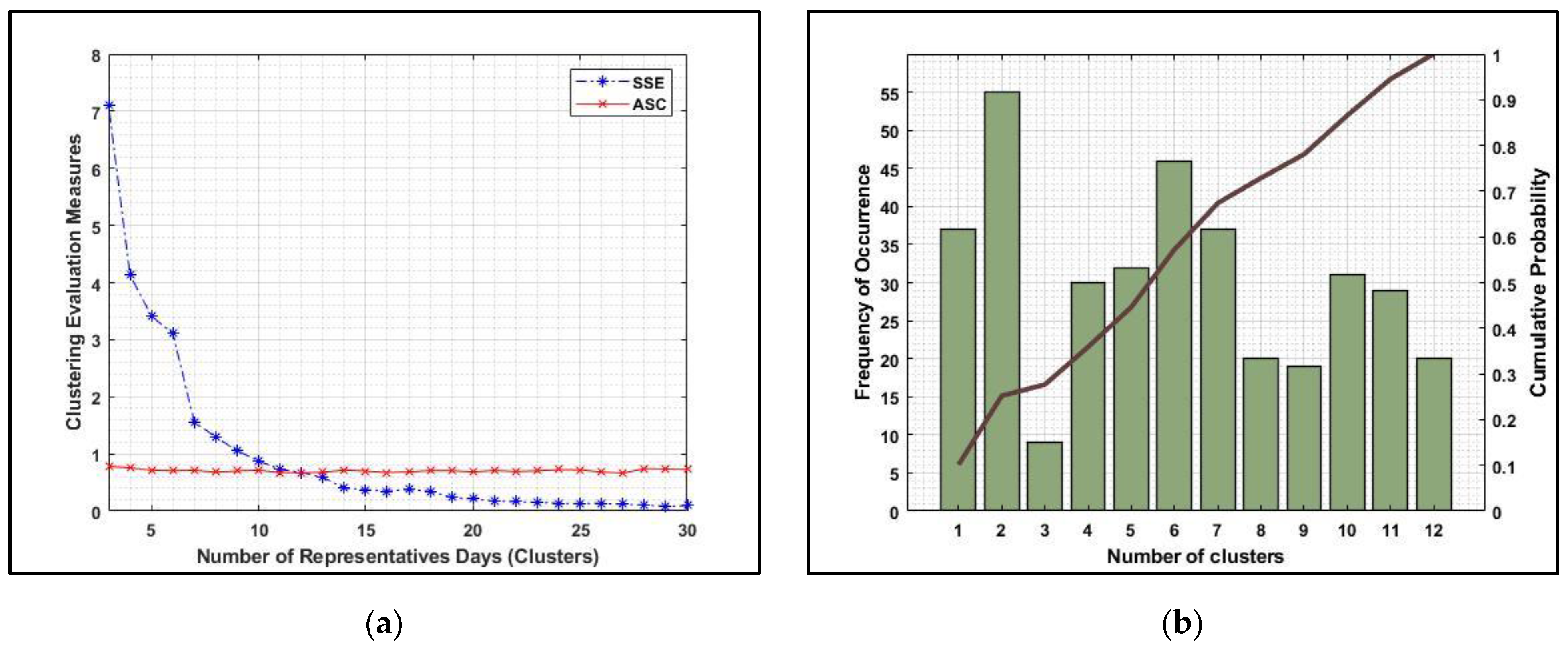
The primary objective of employing the k-means algorithm is to partition the data into k distinct groups while minimizing the within-group distance. To thoroughly explore the dataset and mitigate the impact of the initial point selection on the clustering outcome, the k-means procedure is iteratively repeated multiple times, specifically 100 times in this case, with diverse initial points (a pool of 50 points for each iteration). This iterative process significantly contributes to enhancing the robustness of the clustering outcomes. The assessment of the resulting clusters involves the use of both external and internal validity indices, which are associated with supervised and unsupervised learning, respectively [51]. Two pertinent unsupervised learning indices are the Average Silhouette Coefficient (ASC) and the Sum of Squares Error (SSE), as described in Equations (31) and (32). These metrics offer insights into the compactness of the clusters and the overall quality of the partitioning, respectively. Additionally, an external validity index known as the Average Power Time Mismatch (APTM) [52], introduced in Equation (33), is used. This index assesses the effectiveness of clustering concerning external criteria, providing a measure of how well clusters align with predefined attributes or classifications.
In the given context, denotes the silhouette coefficient for the data point. Within the formula, signifies the average distance from the point to all other points within the same cluster, while represents the average distance from the point to all points in clusters other than its own. The user-defined parameter indicates the number of clusters, and the function pertains to the within-group Euclidean distance between the point in the cluster and its centroid . Additionally, corresponds to the total number of days in a year.
6.5. Representative Selection Stage
The ASC, SSE, and APTM indices can be assigned weights, as indicated in Equation (34), to assess proximity and facilitate the selection of the optimal number of clusters [52].
where represents a hypothetical load profile, while refers to the actual load profile for the hour and day. The variable serves as a scaling factor that increments by 0.1 within a range from 0 to 1. In the representation of the load profile spanning days (i.e., 365 days), a specific number of clusters are employed. Each cluster is characterized by its centroid, which serves as a representative point for that cluster. When the centroid corresponds to an actual hour in the original data, the daily profile associated with that hour is used to represent the entire cluster. However, if the centroid does not align with an actual hour in the original dataset, the nearest actual hour is chosen to represent the cluster. Consequently, the daily profile linked to the selected nearest hour is utilized as the representative profile for that particular cluster. This approach ensures that each cluster is effectively represented by a meaningful and interpretable daily profile, whether derived directly from a centroid or approximated through the nearest available hour in the original data.
6.6. Clustering Results
The k-means algorithm is employed to group similar days within each profile. This process is iteratively repeated a substantial number of times (250 times) with varied initial points (50 points each time). This repetition is aims to minimize the impact of the initial point selection on the resulting groups. The evaluation of clusters involves both supervised and unsupervised measures, as expressed in Equations (31)–(33). Cluster evaluation results for PV irradiance, PV temperature, and load profile are depicted in Figure 3a, Figure 4a and Figure 5a. To determine the optimal number of clusters for each profile, Equation (34) is utilized. Following a cumulative total of (250 × 11) iterations, each initiated with 50 different starting points for each profile, the outcomes reveal that the optimal number of clusters for PV irradiance, PV temperature, and load profile are 22 clusters (representing 22 days), 13 clusters (representing 13 days), and 12 clusters (representing 12 days), respectively, as illustrated in Figure 3b, Figure 4b and Figure 5b. Consequently, these identified clusters are proposed as the most suitable groupings for the respective profiles based on this research.
6.7. Profiles in Monte Carlo Simulation
The representative daily profiles, established through the previous clustering procedure as 22, 13, and 12 clusters, are utilized in each iteration of the Monte Carlo simulation. The selection of these profiles is based on their cumulative probabilities, as depicted on the right Y-axes of Figure 3b, 4Figure 4b and Figure 5b. Considering that each representative daily load profile is presented in terms of the hourly kW demand as a percentage, a scaling process is applied using the substation peak demand. This scaling operation involves multiplying the percentage hourly kW values of the representative profile by the substation peak load. Subsequently, the scaled profiles are assigned to their corresponding PQ loads, as shown in Figure 6. In contrast, PV irradiance and temperature are expressed using their actual values, as emphasized in Figure 6.
7. Results and Discussion
This study examines the real Aljouf region grid’s RTH-based approach for installing FCSs; in this network, two synchronous generators, Hail and Arar, are located at buses 1 and 14, respectively, while a standby generator is located at bus 16. The network has twenty-two branches, four transformers, and eight constant PQ loads and nominal base values of 132 kV for voltage and 100 MVA for the apparent power. In the base case, there is a total load of 149.34 MVAR and 571.2 MW. The structure of the Aljouf Transmission Network is shown in Figure 7. Three fast charging stations with a power factor of 0.9 are integrated using the suggested RTH, and the obtained results are contrasted with those of alternative approaches such as the Kepler optimization algorithm (KOA) [53], gold rush optimizer (GRO) [54], grey wolf optimizer (GWO) [55], and spider wasp optimizer (SWO) [56]. For every approach under consideration, the population size, maximum number of iterations, and number of runs are denoted as 20, 100, and 30, respectively. The authors selected these optimizers as they are nature-inspired approaches like the suggested RTH.
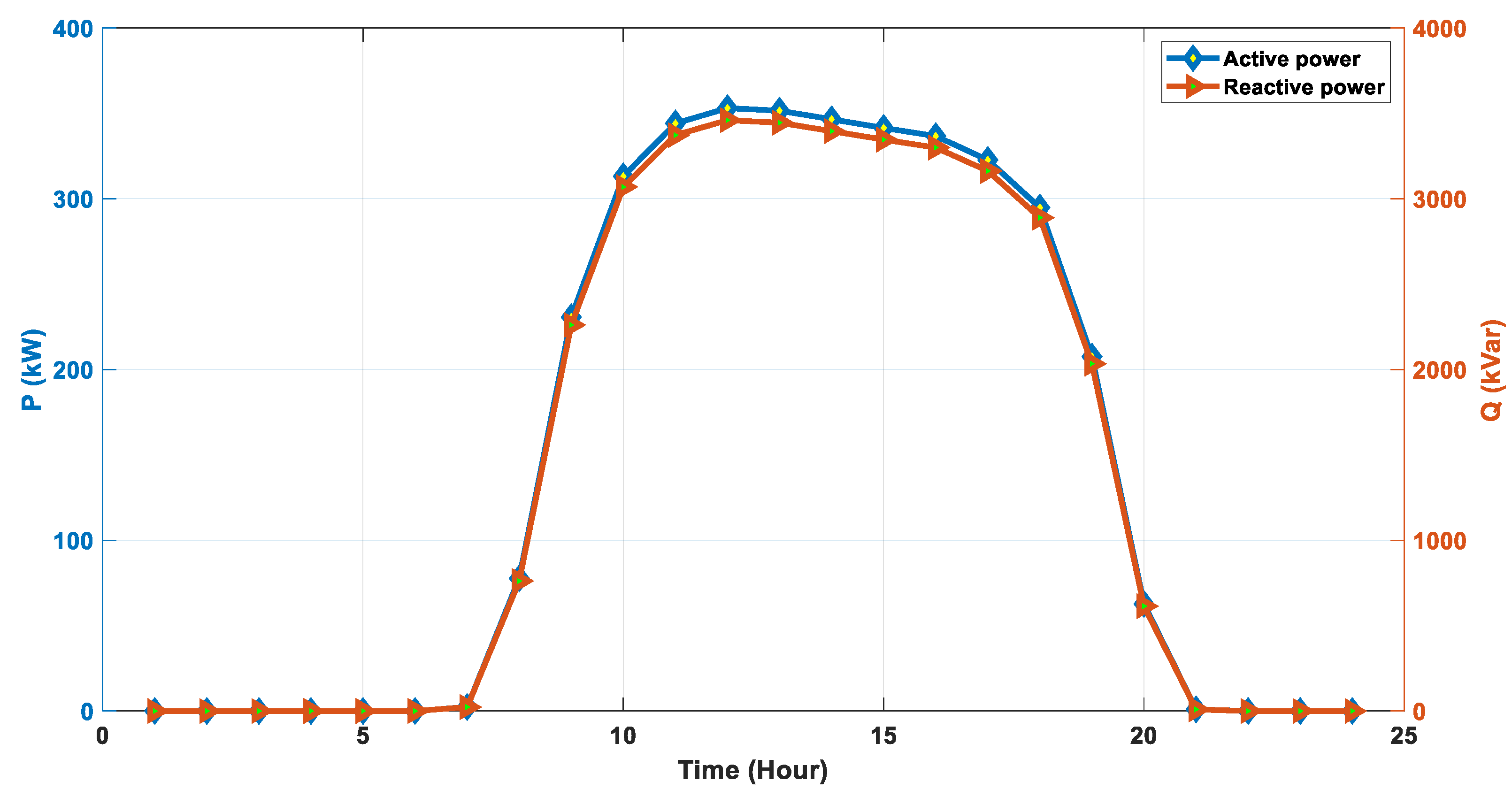
The daily active and reactive generated powers from the PV Sakaka plant are shown in Figure 8. The generation occurred from 7:00 AM to 8:30 PM. Also, the daily profile of the considered demand on the grid is shown in Figure 9, while the daily profiles of active and reactive power generated from the grid are shown in Figure 10.
In order to minimize grid voltage violations, the Aljouf region grid integrates FCSs through the RTH and other methods. Table 1 tabulates the optimal locations and sizes determined for the FCSs that are being considered. The daily voltage deviation of the original network 0.4510 pu. The results contain a fitness function known as the voltage deviation, and it is calculated using Equation (11); moreover, the bus with the maximum voltage and the other with the minimum voltage are tabulated in Table 1 as Max. voltage and Min. voltage, respectively. In the analysis, three FCSs are considered; the maximum power of each one is 25 MW, and it is possible to locate them in all buses except for the slack one (the Hail plant). These limits are identified, and the proposed RTH is responsible for obtaining the optimal active powers, power factors, and reactive powers of the installed FCSs.
Installing three FCSs with capacities of 25 MW, 19.1039 MW, and 10.0272 MW on buses 15, 2, and 13 was advised by the suggested RTH approach. The corresponding reactive power values of the installed FCSs are 12.1081 Mvar, 9.25242 Mvar, and 4.85639 Mvar, respectively. In this case, buses 10 and 6 have the minimum and maximum voltages with values of 0.9902 pu and 1.0674 pu, respectively. This integration yields the lowest network voltage deviation, measuring 0.134346 pu. It is clear that the suggested RTH recommended FCSs with fractional powers; in practice, these values can be rounded to the nearest integer values. By installing 10.3856 MW, 0.4827 MW, and 5.4749 MW on buses 2, 2, and 12, respectively, the GRO comes next and achieves a fitness value of 0.135646 pu. Between bus 13 and bus 7, the minimum and maximum voltages obtained from this integration are 1.017 pu and 1.0466 pu, respectively. Conversely, the KOA is the worst method since it installed 20.5428 MW, 6.71063 MW, and 5.4749 MW FCSs at buses 10, 15, and 15, respectively, to achieve a voltage deviation of 0.148358 pu. In this instance, the minimum and maximum voltages for buses 5 and 14 are 0.9706 pu and 1.0380 pu, respectively. Moreover, the GWO and SWO achieved network voltage deviations of 0.13725 pu and 0.147754 pu, respectively.
In comparison with the others, the suggested RTH demonstrated its effectiveness in obtaining the minimum network voltage deviation of the network by providing the accurate locations and capacities of the integrated FCSs. Additionally, the performance of the suggested RTH is evaluated using a few computed statistical parameters shown in Table 2.
It is evident that the RTH performed better than any of the others, particularly with respect to variance and standard deviation (Std). This supports the suggested approach’s level of performance, which is preferred over the alternatives. Figure 11 shows the voltage violation in relation to the number of iterations for each considered algorithm.
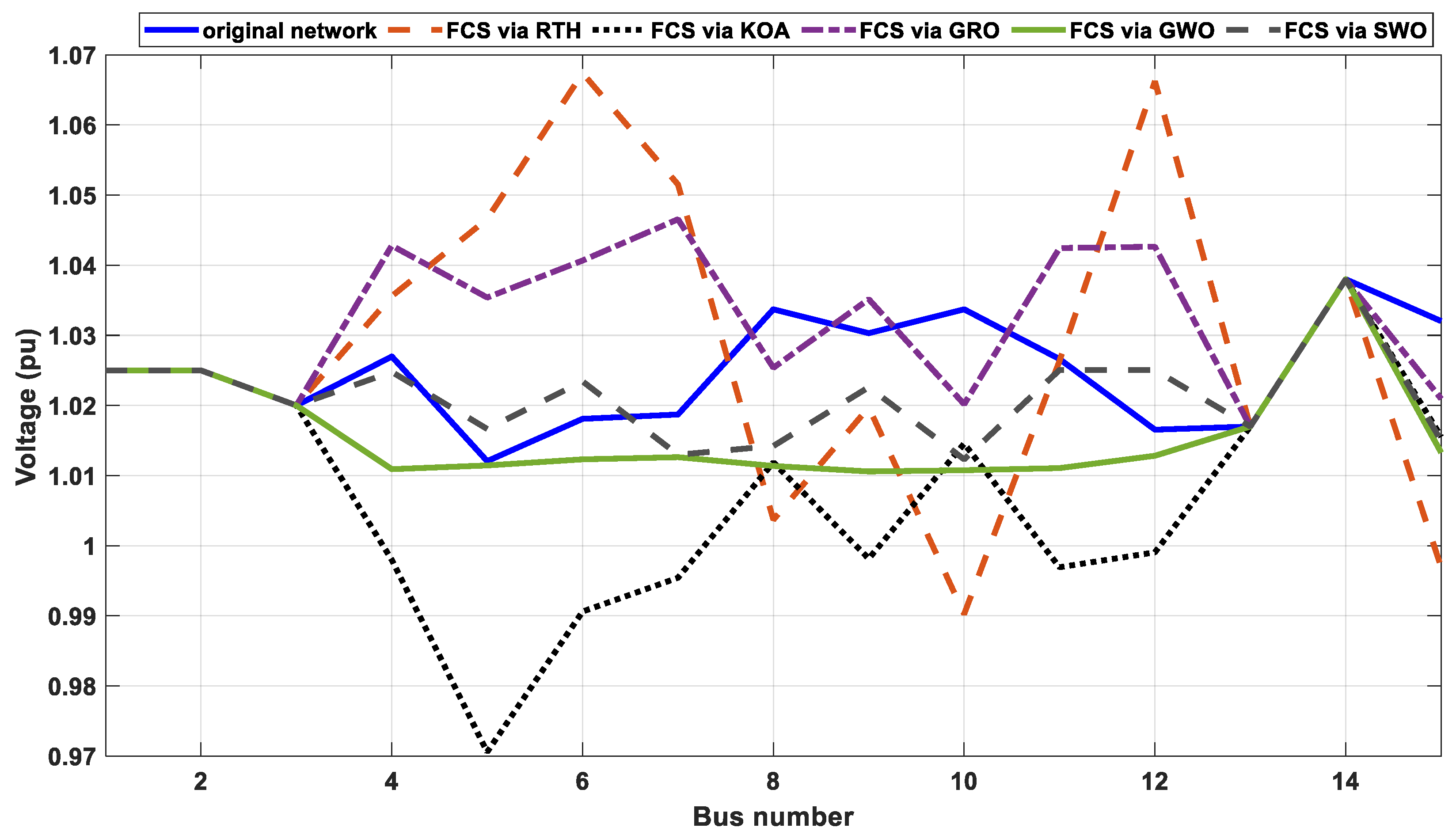
Given that the RTH reached the optimal solution after 50 iterations and the GRO reached the optimal solution after roughly 68 iterations; it is evident that the RTH has a high convergence speed. Conversely, SWO arrived at local solution early on, following ten iterations. Figure 12 displays the network’s daily mean voltage profile both before and after the FCSs were integrated using various techniques. The allowable voltage limits for breaches are within +/− 5 to 10% of the rated value (1 pu), according to IEEE Std 1250–2018 [57]. As a result, the values of the maximum and lowest permitted voltages are 1.1 pu and 0.9 pu, respectively. The voltage pattern of the grid with FCSs whose sizes and locations were assessed using the suggested RTH is within the acceptable limits, as seen in the curves. The curves are the same at buses 1–3 as they are in the same region with a voltage of 380 kV; the plots on tires 13–14 are the also same as they have generators that may have a greater effect than the installed FCSs.
The obtained results demonstrate the effectiveness of the suggested RTH approach in minimizing grid voltage fluctuations by installing FCSs in the Aljouf Transmission Grid.
8. Conclusions
This study suggests a novel approach to address the issue of integrating fast charging stations (FCSs) into the Aljouf Transmission Grid. The approach incorporates a recent metaheuristic approach: the Red-Tailed Hawk Algorithm (RTH). The recommended method found the ideal FCS locations and capacities to reduce network voltage violation over a 24 h period. The RTH’s advantages that allow it to solve the problem under study are its high rate of convergence and ability to forego local solutions. In addition to two conventional generating plants and a standby generator, the Aljouf region’ grid is analyzed taking into consideration the 300 MW Sakaka PV plant. Other algorithms, the Kepler optimization algorithm (KOA), gold rush optimizer (GRO), grey wolf optimizer (GWO), and spider wasp optimizer (SWO), are compared with the proposed method. The k-means approach is utilized to prepare each dataset by reducing its complexity through the application of a PCA. Using the k-means clustering algorithm, each dataset is divided into k unique clusters which are then assessed using both internal and external validity indices. To choose the ideal number of clusters, the values of these indices are weighted. Additionally, each data set’s daily profile is determined in a probabilistic manner by the application of a Monte Carlo simulation (MCS).
The following findings are obtained:
- By attaining the lowest fitness value of 0.134346, the RTH was able to reduce the network voltage deviation by 29.79% from its initial value.
- With a 29.66% reduction in network voltage violation compared to the original network, the GRO ranked second in terms of mitigation.
- With a 0.148358 pu and a 28.38% reduction in the new fitness value over the initial one, the KOA achieved the lowest rank.
The results validated the competency of the proposed approach in integrating FCSs into an actual transmission grid by determining the optimal locations and sizes for them while minimizing voltage variations.
Author Contributions
Conceptualization, S.M.A. and A.F.; methodology, S.M.A.; software, S.M.A. and A.F.; formal analysis, S.M.A.; investigation, S.M.A. and A.F.; resources, S.M.A. and A.F.; data curation, S.M.A. and A.F.; writing—original draft preparation, S.M.A. and A.F.; writing—review and editing, S.M.A. and A.F.; visualization, S.M.A. and A.F.; supervision, S.M.A.; project administration, S.M.A.; funding acquisition, S.M.A. All authors have read and agreed to the published version of the manuscript.
Funding
This research was funded by the Prince Nawaf bin Abdelaziz Chair for Sustainable Development in collaboration with the Deanship of Scientific Research at Jouf University under grant No (DSR2023-Prince Nawaf bin Abdulaziz Chair-02).
Data Availability Statement
The original contributions presented in the study are included in the article, further inquiries can be directed to the corresponding author.
Conflicts of Interest
The authors declare no conflict of interest.
References
- Fazelpour, F.; Vafaeipour, M.; Rahbari, O.; Rosen, M.A. Intelligent optimization to integrate a plug-in hybrid electric vehicle smart parking lot with renewable energy resources and enhance grid characteristics. Energy Convers. Manag. 2014, 77, 250–261. [Google Scholar] [CrossRef]
- Amini, M.H.; Boroojeni, K.G.; Wang, C.J.; Nejadpak, A.; Iyengar, S.S.; Karabasoglu, O. Effect of electric vehicle parking lots’ charging demand as dispatchable loads on power systems loss. In Proceedings of the 2016 IEEE International Conference on Electro Information Technology (EIT), Grand Forks, ND, USA, 19–21 May 2016; IEEE: Piscataway, NJ, USA, 2016; pp. 0499–0503. [Google Scholar]
- Xu, N.Z.; Chung, C.Y. Uncertainties of EV charging and effects on well-being analysis of generating systems. IEEE Trans. Power Syst. 2014, 30, 2547–2557. [Google Scholar] [CrossRef]
- Ahmad, F.; Bilal, M. Allocation of plug-in electric vehicle charging station with integrated solar powered distributed generation using an adaptive particle swarm optimization. Electr. Eng. 2023, 1–14. [Google Scholar] [CrossRef]
- Ghanaei, N.; Moghaddam, M.S.; Alibeaki, E.; Salehi, N.; Davarzani, R. Bi-level stochastic optimization model of smart distribution grids considering the transmission network to reduce vulnerability. Energy Syst. 2023, 1–34. [Google Scholar] [CrossRef]
- Ibtihel Ben, G.; de Nunzio, G.; Sciarretta, A. Optimal Placement of Fast Charging Infrastructure for Electric Vehicles: An Optimal Routing and Spatial Clustering Approach. In Proceedings of the 26th IEEE International Conference on Intelligent Transportation Systems (ITSC 2023), Bilbao, Spain, 24–28 September 2023. [Google Scholar]
- Kumar, N.; Kumar, T.; Nema, S.; Thakur, T. Reliability oriented techno-economic assessment of fast charging stations with photovoltaic and battery systems in paired distribution & urban network. J. Energy Storage 2023, 72, 108814. [Google Scholar]
- Zhou, G.; Dong, Q.; Zhao, Y.; Wang, H.; Jian, L.; Jia, Y. Bilevel optimization approach to fast charging station planning in electrified transportation networks. Appl. Energy 2023, 350, 121718. [Google Scholar] [CrossRef]
- Singh, K.; Mistry, K.D.; Patel, H.G. Optimal Placement of Electric Vehicle Charging Station and DG in a Distribution System for Loss Minimization. In Proceedings of the 2023 IEEE 3rd International Conference on Sustainable Energy and Future Electric Transportation (SEFET), Bhubaneswar, India, 9–12 August 2023; IEEE: Piscataway, NJ, USA, 2023; pp. 1–6. [Google Scholar]
- Alshareef, S.M.; Fathy, A. Efficient Red Kite Optimization Algorithm for Integrating the Renewable Sources and Electric Vehicle Fast Charging Stations in Radial Distribution Networks. Mathematics 2023, 11, 3305. [Google Scholar] [CrossRef]
- Kapoor, A.; Patel, V.S.; Sharma, A.; Mohapatra, A. Optimal Planning of Fast EV Charging Stations in a Coupled Transportation and Electrical Power Distribution Network. IEEE Trans. Autom. Sci. Eng. 2023, 1–11. [Google Scholar] [CrossRef]
- Li, Y.; Su, S.; Zhang, M.; Liu, Q.; Nie, X.; Xia, M.; Micu, D.D. Multi-Agent Graph Reinforcement Learning Method for Electric Vehicle on-Route Charging Guidance in Coupled Transportation Electrification. IEEE Trans. Sustain. Energy 2023, 15, 1180–1193. [Google Scholar] [CrossRef]
- Draz, A.; Othman, A.M.; El-Fergany, A.A. State-of-the-Art with Numerical Analysis on Electric Fast Charging Stations: Infrastructures, Standards, Techniques, and Challenges. Renew. Energy Focus 2023, 47, 100499. [Google Scholar] [CrossRef]
- Zhou, G.; Zhao, Y.; Lai, C.S.; Jia, Y. A profitability assessment of fast-charging stations under vehicle-to-grid smart charging operation. J. Clean. Prod. 2023, 428, 139014. [Google Scholar] [CrossRef]
- Gupta, R.S.; Anand, Y.; Tyagi, A.; Anand, S. Sustainable charging station allocation in the distribution system for electric vehicles considering technical, economic, and societal factors. J. Energy Storage 2023, 73, 109052. [Google Scholar] [CrossRef]
- Ren, H.; Zhou, Y.; Wen, F.; Liu, Z. Optimal dynamic power allocation for electric vehicles in an extreme fast charging station. Appl. Energy 2023, 349, 121497. [Google Scholar] [CrossRef]
- Bhadoriya, J.S.; Gupta, A.R.; Kumar, A.; Ray, R.; Maini, S. Enhancement of the distribution network in the presence of EV charging stations augmented by distributed generation. Electr. Eng. 2023, 105, 3703–3717. [Google Scholar] [CrossRef]
- Napoli, G.; Polimeni, A.; Micari, S.; Andaloro, L.; Antonucci, V. Optimal allocation of electric vehicle charging stations in a highway network: Part 1. Methodology and test application. J. Energy Storage 2020, 27, 101102. [Google Scholar] [CrossRef]
- Kong, W.; Luo, Y.; Feng, G.; Li, K.; Peng, H. Optimal location planning method of fast charging station for electric vehicles considering operators, drivers, vehicles, traffic flow and power grid. Energy 2019, 186, 115826. [Google Scholar] [CrossRef]
- Hadian, E.; Akbari, H.; Farzinfar, M.; Saeed, S. Optimal allocation of electric vehicle charging stations with adopted smart charging/discharging schedule. IEEE Access 2020, 8, 196908–196919. [Google Scholar] [CrossRef]
- Liu, L.; Zhang, Y.; Da, C.; Huang, Z.; Wang, M. Optimal allocation of distributed generation and electric vehicle charging stations based on intelligent algorithm and bi-level programming. Int. Trans. Electr. Energy Syst. 2020, 30, e12366. [Google Scholar] [CrossRef]
- Zeb, M.Z.; Imran, K.; Khattak, A.; Janjua, A.K.; Pal, A.; Nadeem, M.; Zhang, J.; Khan, S. Optimal placement of electric vehicle charging stations in the active distribution network. IEEE Access 2020, 8, 68124–68134. [Google Scholar] [CrossRef]
- Pal, A.; Bhattacharya, A.; Chakraborty, A.K. Allocation of electric vehicle charging station considering uncertainties. Sustain. Energy Grids Netw. 2021, 25, 100422. [Google Scholar] [CrossRef]
- Ma, T.-Y.; Xie, S. Optimal fast charging station locations for electric ridesharing with vehicle-charging station assignment. Transp. Res. Part D Transp. Environ. 2021, 90, 102682. [Google Scholar] [CrossRef]
- Ahmad, F.; Iqbal, A.; Ashraf, I.; Marzband, M.; Khan, I. Optimal location of electric vehicle charging station and its impact on distribution network: A review. Energy Rep. 2022, 8, 2314–2333. [Google Scholar] [CrossRef]
- Deb, S.; Tammi, K.; Kalita, K.; Mahanta, P. Charging station placement for electric vehicles: A case study of Guwahati city, India. IEEE Access 2019, 7, 100270–100282. [Google Scholar] [CrossRef]
- Campaña, M.; Inga, E.; Cárdenas, J. Optimal sizing of electric vehicle charging stations considering urban traffic flow for smart cities. Energies 2021, 14, 4933. [Google Scholar] [CrossRef]
- Khan, W.; Ahmad, F.; Alam, M.S. Fast EV charging station integration with grid ensuring optimal and quality power exchange. Eng. Sci. Technol. Int. J. 2019, 22, 143–152. [Google Scholar] [CrossRef]
- Shukla, A.; Verma, K.; Kumar, R. Multi-objective synergistic planning of EV fast-charging stations in the distribution system coupled with the transportation network. IET Gener. Transm. Distrib. 2019, 13, 3421–3432. [Google Scholar] [CrossRef]
- Jiang, X.; Zhao, L.; Cheng, Y.; Wei, S.; Jin, Y. Optimal configuration of electric vehicles for charging stations under the fast power supplement mode. J. Energy Storage 2022, 45, 103677. [Google Scholar] [CrossRef]
- Hashemian, S.N.; Latify, M.A.; Yousefi, G.R. PEV fast-charging station sizing and placement in coupled transportation-distribution networks considering power line conditioning capability. IEEE Trans. Smart Grid 2020, 11, 4773–4783. [Google Scholar] [CrossRef]
- Geetha, B.T.; Prakash, A.; Jeyasudha, S.; Dinakaran, K.P. Hybrid approach based combined allocation of electric vehicle charging stations and capacitors in distribution systems. J. Energy Storage 2023, 72, 108273. [Google Scholar] [CrossRef]
- Zhou, G.; Zhu, Z.; Luo, S. Location optimization of electric vehicle charging stations: Based on cost model and genetic algorithm. Energy 2022, 247, 123437. [Google Scholar] [CrossRef]
- Rajesh, P.; Shajin, F.H. Optimal allocation of EV charging spots and capacitors in distribution network improving voltage and power loss by Quantum-Behaved and Gaussian Mutational Dragonfly Algorithm (QGDA). Electr. Power Syst. Res. 2021, 194, 107049. [Google Scholar] [CrossRef]
- Wu, X.; Feng, Q.; Bai, C.; Lai, C.S.; Jia, Y.; Lai, L.L. A novel fast-charging stations locational planning model for electric bus transit system. Energy 2021, 224, 120106. [Google Scholar] [CrossRef]
- He, Y.; Kockelman, K.M.; Perrine, K.A. Optimal locations of US fast charging stations for long-distance trip completion by battery electric vehicles. J. Clean. Prod. 2019, 214, 452–461. [Google Scholar] [CrossRef]
- Pal, A.; Bhattacharya, A.; Chakraborty, A.K. Placement of public fast-charging station and solar distributed generation with battery energy storage in distribution network considering uncertainties and traffic congestion. J. Energy Storage 2021, 41, 102939. [Google Scholar] [CrossRef]
- Suhail, M.; Akhtar, I.; Kirmani, S. Objective functions and infrastructure for optimal placement of electrical vehicle charging station: A comprehensive survey. IETE J. Res. 2023, 69, 5250–5260. [Google Scholar] [CrossRef]
- Akhmetshin, A.R.; Suslov, K.V.; Olentsevich, V.A.; Gladkikh, V.A.; Karlina, A.I.; Baraboshkin, K.A. The impact of the passage of long-distance trains on the required electrical capacity of the transport infrastructure facilities of the Eastern polygon of Railways. In Journal of Physics: Conference Series; IOP Publishing: Bristol, UK, 2022; Volume 2176, p. 012038. [Google Scholar]
- Moghaddam, A.A.; Seifi, A.; Niknam, T. Multi-operation management of a typical micro-grids using Particle Swarm Optimization: A comparative study. Renew. Sustain. Energy Rev. 2012, 16, 1268–1281. [Google Scholar] [CrossRef]
- Fathy, A.; Kaaniche, K.; Alanazi, T.M. Recent approach based social spider optimizer for optimal sizing of hybrid PV/wind/battery/diesel integrated microgrid in aljouf region. IEEE Access 2020, 8, 57630–57645. [Google Scholar] [CrossRef]
- Roe, C.; Meliopoulos, A.P.; Meisel, J.; Overbye, T. Power system level impacts of plug-in hybrid electric vehicles using simulation data. In Proceedings of the 2008 IEEE Energy 2030 Conference, Atlanta, GA, USA, 17–18 November 2008; IEEE: Piscataway, NJ, USA, 2008; pp. 1–6. [Google Scholar]
- Ferahtia, S.; Houari, A.; Rezk, H.; Djerioui, A.; Machmoum, M.; Motahhir, S.; Ait-Ahmed, M. Red-tailed hawk algorithm for numerical optimization and real-world problems. Sci. Rep. 2023, 13, 12950. [Google Scholar] [CrossRef]
- Proedrou, E. A comprehensive review of residential electricity load profile models. IEEE Access 2021, 9, 12114–12133. [Google Scholar] [CrossRef]
- Li, H.; Wang, Z.; Hong, T.; Parker, A.; Neukomm, M. Characterizing patterns and variability of building electric load profiles in time and frequency domains. Appl. Energy 2021, 291, 116721. [Google Scholar] [CrossRef]
- Zhong, S.; Tam, K.-S. Hierarchical classification of load profiles based on their characteristic attributes in frequency domain. IEEE Trans. Power Syst. 2014, 30, 2434–2441. [Google Scholar] [CrossRef]
- Herraiz-Cañete, Á.; Ribó-Pérez, D.; Bastida-Molina, P.; Gómez-Navarro, T. Forecasting energy demand in isolated rural communities: A comparison between deterministic and stochastic approaches. Energy Sustain. Dev. 2022, 66, 101–116. [Google Scholar] [CrossRef]
- ElNozahy, M.S.; Salama, M.M.A.; Seethapathy, R. A probabilistic load modelling approach using clustering algorithms. In Proceedings of the 2013 IEEE Power & Energy Society General Meeting, Vancouver, BC, Canada, 21–25 July 2013; IEEE: Piscataway, NJ, USA, 2013; pp. 1–5. [Google Scholar]
- Grigg, C.; Wong, P.; Albrecht, P.; Allan, R.; Bhavaraju, M.; Billinton, R.; Chen, Q.; Fong, C.; Haddad, S.; Kuruganty, S.; et al. The IEEE reliability test system-1996. A report prepared by the reliability test system task force of the application of probability methods subcommittee. IEEE Trans. Power Syst. 1999, 14, 1010–1020. [Google Scholar] [CrossRef]
- Panapakidis, I.P.; Alexiadis, M.C.; Papagiannis, G.K. Enhancing the clustering process in the category model load profiling. IET Gener. Transm. Distrib. 2015, 9, 655–665. [Google Scholar] [CrossRef]
- Kovács, F.; Legány, C.; Babos, A. Cluster validity measurement techniques. In Proceedings of the 6th International Symposium of Hungarian Researchers on Computational Intelligence, Budapest, Hungary, 18–19 November 2005; Volume 35. [Google Scholar]
- Alshareef, S.M.; Morsi, W.G. Probabilistic commercial load profiles at different climate zones. In Proceedings of the 2017 IEEE Electrical Power and Energy Conference (EPEC), Saskatoon, SK, Canada, 22–25 October 2017; IEEE: Piscataway, NJ, USA, 2017; pp. 1–7. [Google Scholar]
- Abdel-Basset, M.; Mohamed, R.; Azeem, S.A.A.; Jameel, M.; Abouhawwash, M. Kepler optimization algorithm: A new metaheuristic algorithm inspired by Kepler’s laws of planetary motion. Knowl.-Based Syst. 2023, 268, 110454. [Google Scholar] [CrossRef]
- Zolf, K. Gold rush optimizer: A new population-based metaheuristic algorithm. Oper. Res. Decis. 2023, 33, 113–150. [Google Scholar] [CrossRef]
- Mirjalili, S.; Mirjalili, S.M.; Lewis, A. Grey wolf optimizer. Adv. Eng. Softw. 2014, 69, 46–61. [Google Scholar] [CrossRef]
- Abdel-Basset, M.; Mohamed, R.; Jameel, M.; Abouhawwash, M. Spider wasp optimizer: A novel meta-heuristic optimization algorithm. Artif. Intell. Rev. 2023, 56, 11675–11738. [Google Scholar] [CrossRef]
- Blanco, C.; Paz, F.; Zurbriggen, I.G.; Garcia, P.; Ordonez, M. Distributed islanding detection in multisource dc microgrids: Pilot signal cancelation. IEEE Access 2022, 10, 78370–78383. [Google Scholar] [CrossRef]
Figure 1.
Flowchart of RTH.

Figure 2.
Total variance explained by the first five principal components.
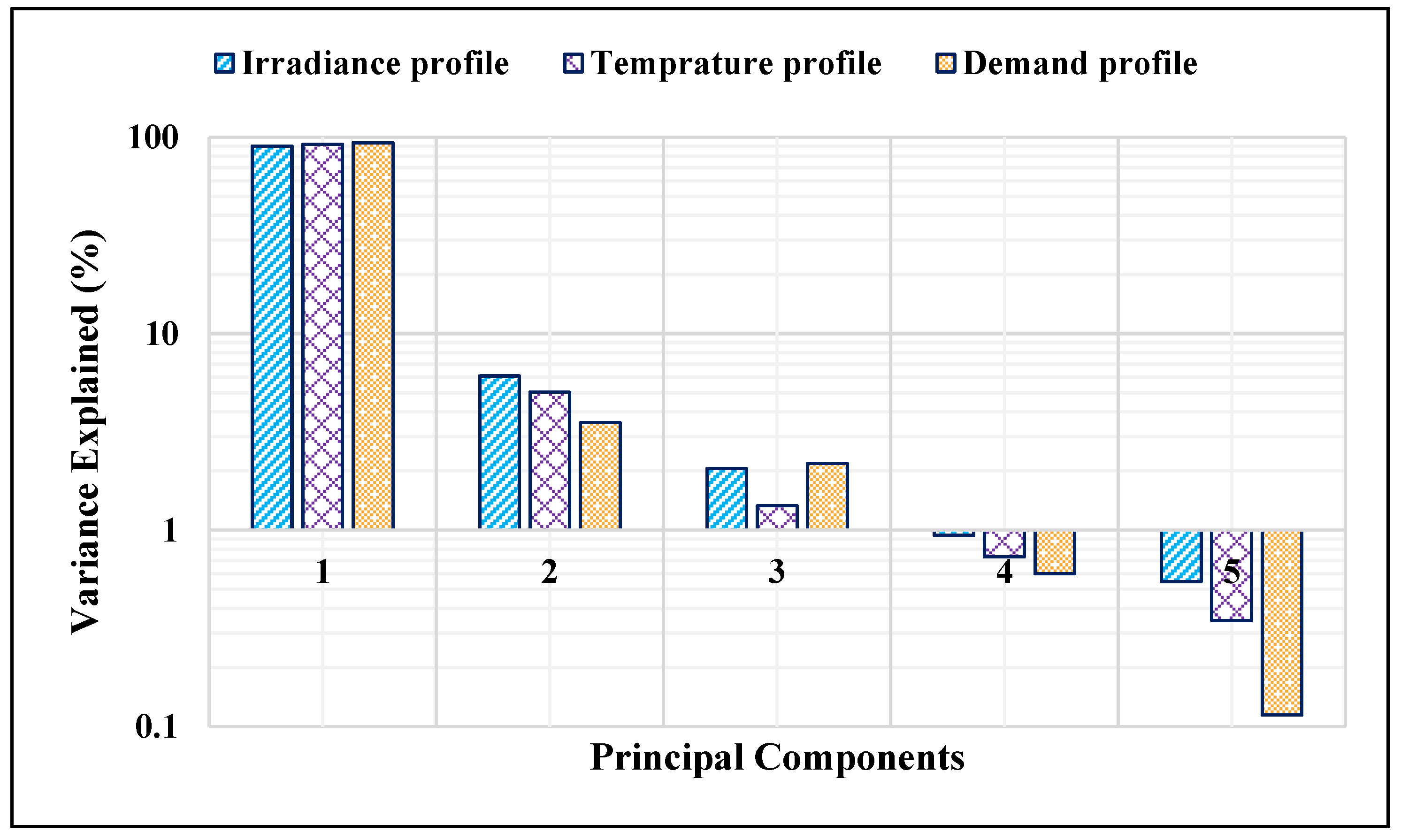
Figure 3.
Clustering assessment for solar irradiance. (a) Results of supervised and unsupervised indices. (b) Frequency of the occurrence of the proposed number of clusters as well as their cumulative distribution function (the right side of the y-axis).
Figure 3.
Clustering assessment for solar irradiance. (a) Results of supervised and unsupervised indices. (b) Frequency of the occurrence of the proposed number of clusters as well as their cumulative distribution function (the right side of the y-axis).
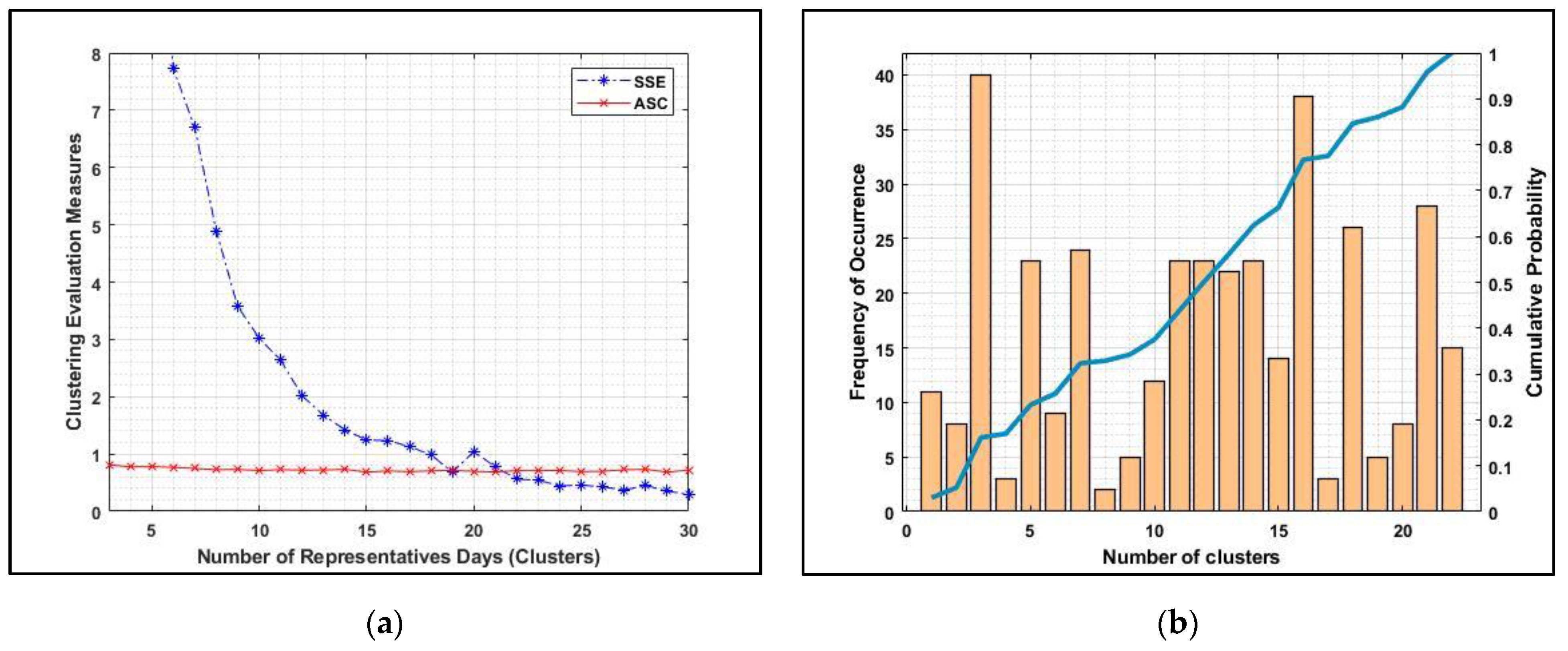
Figure 4.
Clustering assessment for PV temperature. (a) Results of supervised and unsupervised indices. (b) Frequency of occurrence of the proposed number of clusters as well as their cumulative distribution function (the right side of the y-axis).
Figure 4.
Clustering assessment for PV temperature. (a) Results of supervised and unsupervised indices. (b) Frequency of occurrence of the proposed number of clusters as well as their cumulative distribution function (the right side of the y-axis).

Figure 5.
Clustering assessment for substation profile. (a) Results of supervised and unsupervised indices. (b) Frequency of occurrence of proposed number of clusters as well as their cumulative distribution function (the right side of the y-axis).
Figure 5.
Clustering assessment for substation profile. (a) Results of supervised and unsupervised indices. (b) Frequency of occurrence of proposed number of clusters as well as their cumulative distribution function (the right side of the y-axis).
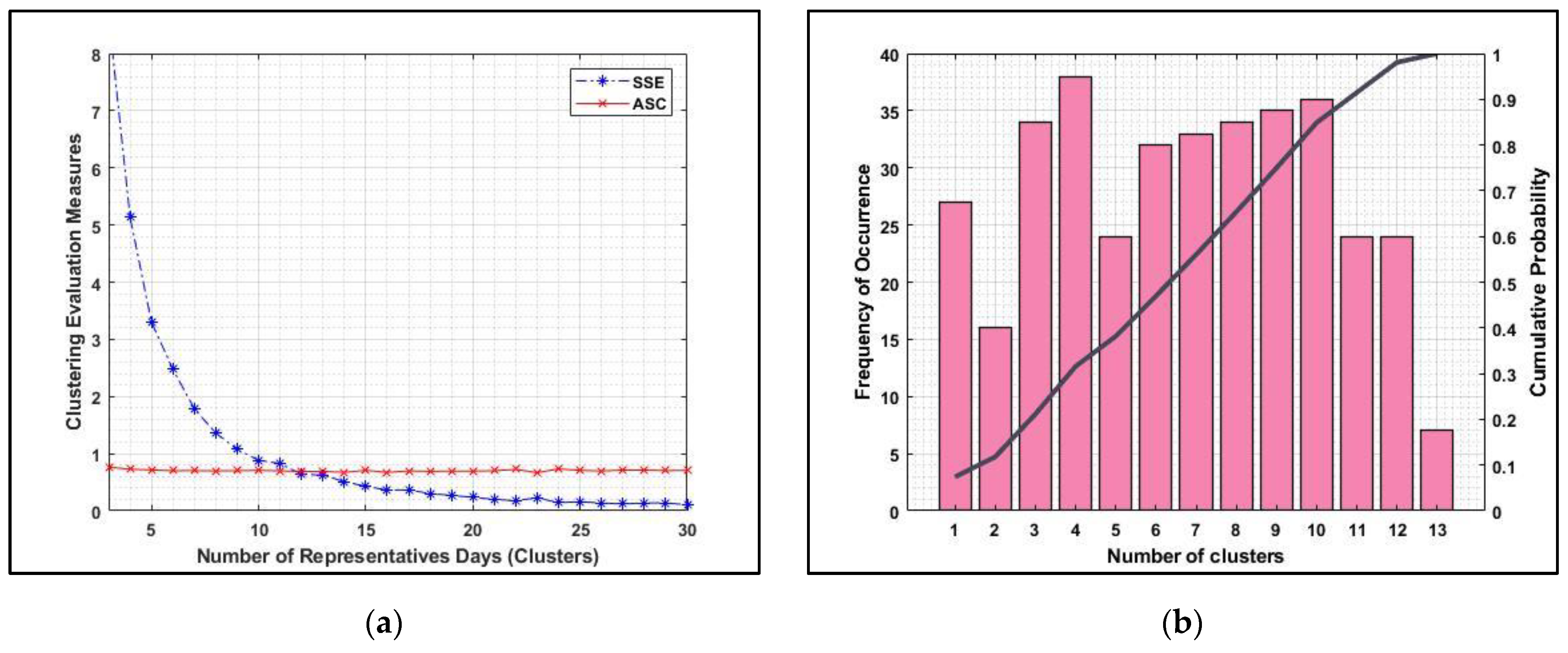
Figure 6.
Max., min., and quantile values of profiles of the proposed clusters for solar irradiance, PV temperature, and substation.
Figure 6.
Max., min., and quantile values of profiles of the proposed clusters for solar irradiance, PV temperature, and substation.

Figure 7.
Aljouf Transmission Grid.

Figure 8.
Daily profile of PV Sakaka plant generation.

Figure 9.
Daily profile of demand.
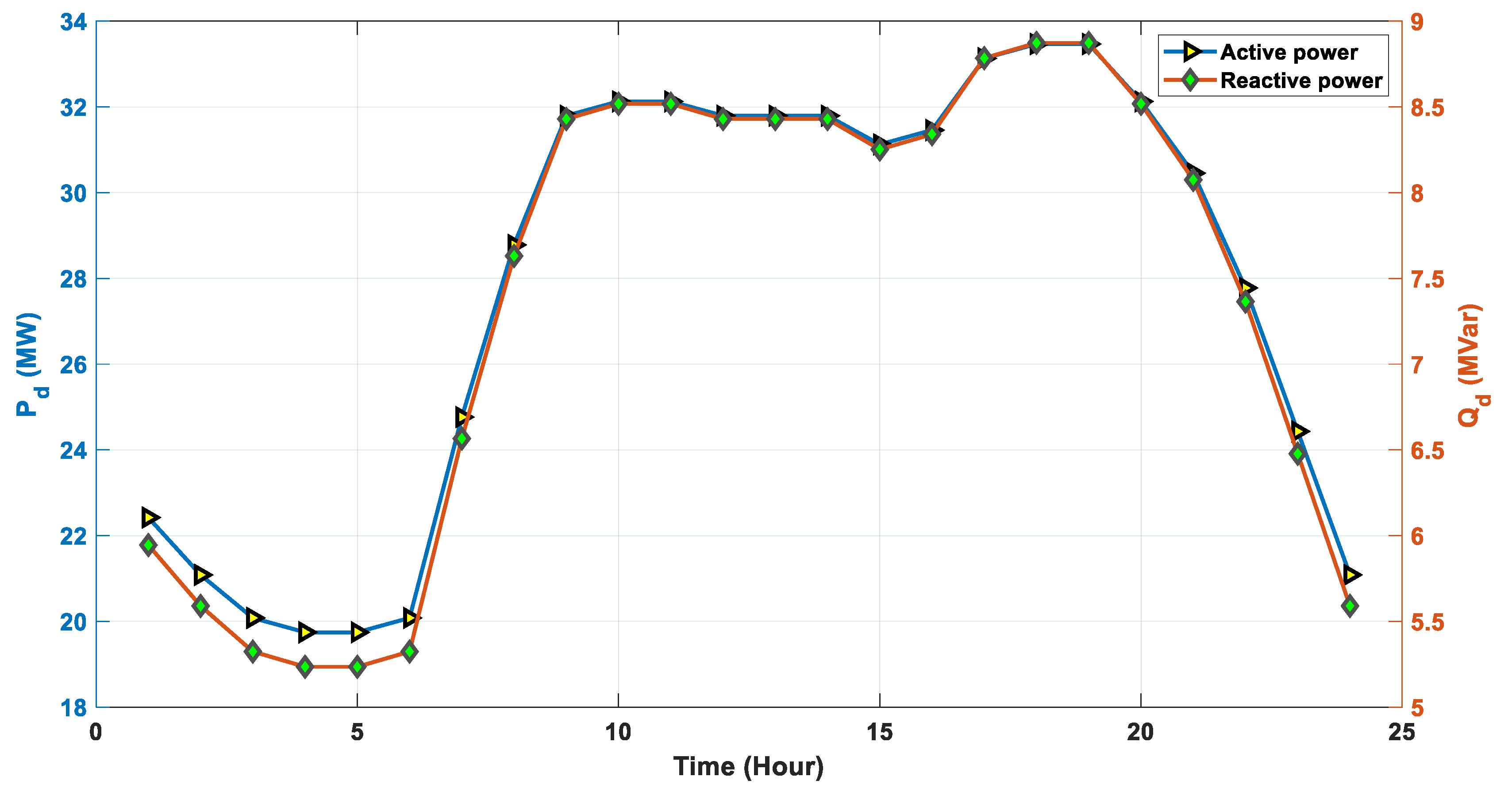
Figure 10.
Daily profile of Aljouf network generation.
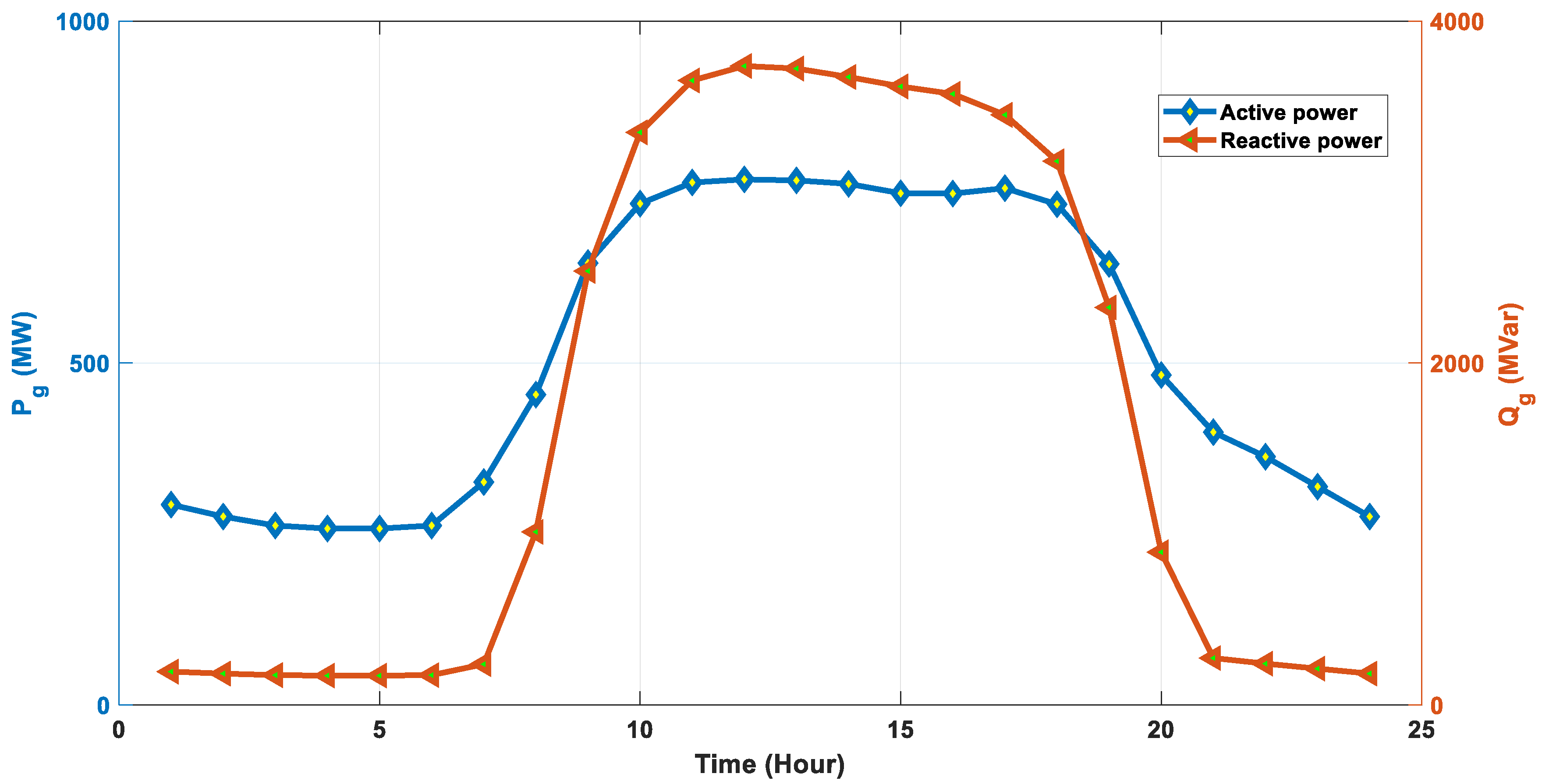
Figure 11.
Voltage violation in relation to the number of iterations for each algorithm under consideration.
Figure 11.
Voltage violation in relation to the number of iterations for each algorithm under consideration.
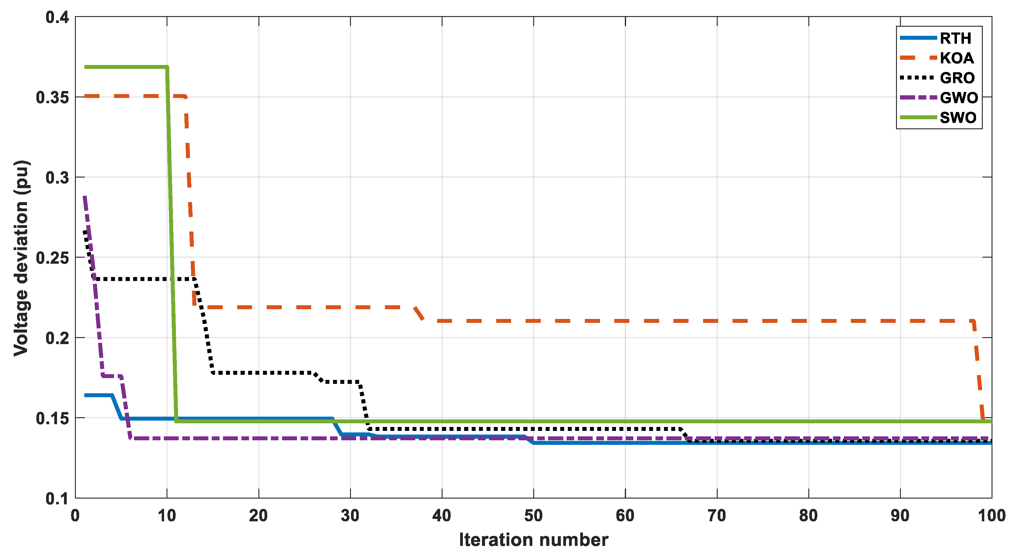
Figure 12.
Mean daily voltage profile of Aljouf Transmission Network.

Table 1.
Optimal FCS locations and sizes under consideration for integration into the Aljouf Transmission Network.
Table 1.
Optimal FCS locations and sizes under consideration for integration into the Aljouf Transmission Network.
| RTH | KOA | GRO | GWO | SWO | ||
|---|---|---|---|---|---|---|
| First fast charging station | P (MW) | 25 | 20.5428 | 10.3856 | 16.2059 | 3.4559 |
| Q (Mvar) | 12.1081 | 9.94933 | 5.03 | 7.8489 | 1.67377 | |
| Place | 15 | 10 | 2 | 15 | 15 | |
| Second fast charging station | P (MW) | 19.1039 | 6.71063 | 0.4827 | 3.06014 | 14.7409 |
| Q (Mvar) | 9.25242 | 3.25011 | 0.2338 | 1.4821 | 7.13935 | |
| Place | 2 | 15 | 2 | 15 | 10 | |
| Third fast charging station | P (MW) | 10.0272 | 25 | 5.4749 | 10.7758 | 21.2383 |
| Q (Mvar) | 4.85639 | 12.1081 | 2.6516 | 5.219 | 10.2862 | |
| Place | 13 | 15 | 12 | 2 | 12 | |
| Voltage deviation (pu) | 0.134346 | 0.148358 | 0.135646 | 0.13725 | 0.147754 | |
| Max. voltage (pu)/place | 1.0674/(6) | 1.0380/(14) | 1.0466/(7) | 1.0380/(14) | 1.0380/(14) | |
| Min. voltage (pu)/place | 0.9902/(10) | 0.9706/(5) | 1.0170/(13) | 1.0106/(9) | 1.0123/(10) | |
Table 2.
Statistical parameters of all approaches under consideration.
| Best | Worst | Average | Variance | Std | |
|---|---|---|---|---|---|
| RTH | 0.1322 | 0.1616 | 0.1396 | 0.0006 | 0.0049 |
| KOA | 0.1484 | 0.2961 | 0.1934 | 0.0325 | 0.0368 |
| GRO | 0.1356 | 0.1551 | 0.1449 | 0.0006 | 0.0050 |
| GWO | 0.1373 | 0.1846 | 0.1455 | 0.0018 | 0.0086 |
| SWO | 0.1478 | 0.3546 | 0.2405 | 0.0912 | 0.0616 |
Disclaimer/Publisher’s Note: The statements, opinions and data contained in all publications are solely those of the individual author(s) and contributor(s) and not of MDPI and/or the editor(s). MDPI and/or the editor(s) disclaim responsibility for any injury to people or property resulting from any ideas, methods, instructions or products referred to in the content. |
© 2024 by the authors. Licensee MDPI, Basel, Switzerland. This article is an open access article distributed under the terms and conditions of the Creative Commons Attribution (CC BY) license (https://creativecommons.org/licenses/by/4.0/).
Share and Cite
MDPI and ACS Style
Alshareef, S.M.; Fathy, A. Optimal Allocation of Fast Charging Stations on Real Power Transmission Network with Penetration of Renewable Energy Plant. World Electr. Veh. J. 2024, 15, 172. https://doi.org/10.3390/wevj15040172
AMA Style
Alshareef SM, Fathy A. Optimal Allocation of Fast Charging Stations on Real Power Transmission Network with Penetration of Renewable Energy Plant. World Electric Vehicle Journal. 2024; 15(4):172. https://doi.org/10.3390/wevj15040172
Chicago/Turabian StyleAlshareef, Sami M., and Ahmed Fathy. 2024. "Optimal Allocation of Fast Charging Stations on Real Power Transmission Network with Penetration of Renewable Energy Plant" World Electric Vehicle Journal 15, no. 4: 172. https://doi.org/10.3390/wevj15040172