Reassessing the Links between GHG Emissions, Economic Growth, and the UNFCCC: A Difference-in-Differences Approach

Abstract

International climate agreements such as the Kyoto Protocol of 1997 and, more recently, the Paris Climate Agreement are fragile because, at a national level, political constituencies’ value systems may conflict with the goal of reducing greenhouse gas (GHG) emissions to sustainable levels. Proponents cite climate change as the most pressing challenge of our time, contending that international cooperation will play an essential role in addressing this challenge. Political opponents argue that the disproportionate requirements on developed nations to shoulder the financial burden will inhibit their economic growth. We find empirical evidence that both arguments are likely to be correct. We use standard regression techniques to analyze a multi-country dataset of GHG emissions, GDP per capita growth, and other factors. We estimate that after the Kyoto Protocol (KP) entered into force ‘Annex I’ countries reduced GHG emissions on average by roughly 1 million metric tons of CO₂ equivalent (MTCO2e), relative to non-Annex I countries. However, our estimates reveal that these countries also experienced an average reduction in GDP per capita growth rates of around 1–2 percentage points relative to non-Annex I countries.

1. Introduction

The nexus between economic output and the environment has long been a key topic in economic and policy research, particularly with respect to sustainable development goals. It is well understood that economic growth leads to environmental degradation in the early stages of development. By the same token, opponents to environmentally-minded regulations have often argued that such regulations hamper economic growth. As a widely publicized example of this, the current United States president, Donald J. Trump, recently declared that the United States would rescind its participation in the historic Paris Agreement on climate change despite its initial status as one of the leading countries in the agreement. An article from 7 November 2017 by the nationally syndicated American newspaper USA Today reported that after Syria had announced its intent to join the Paris Agreement a week prior, this left the U.S. as the sole country not participating in the Agreement [1]. This has reignited the debate (at least in the U.S.) about the effectiveness of climate agreements in curbing greenhouse gas (GHG) emissions at the alleged expense of economic growth.

This work contributes to this revitalized debate by reassessing the empirical links between economic growth, GHG emissions, and international climate agreements. We utilize an established empirical methodology to estimate the impacts on country-level GHG emissions and gross domestic product (GDP) per capita growth rates of participation in the Kyoto Protocol of the United Nations Framework Convention on Climate Change (UNFCCC). As the world’s first international GHG emissions reduction treaty, the well-known Kyoto Protocol of 1997 (KP) was a major step forward for the UNFCCC, but did not officially enter into force until 2005. ‘Annex I’ parties—that is, those classified as industrialized countries or ‘economies in transition’—were, for the first time, formally committed to reduce GHG emissions via the UNFCCC. To test the impact of this commitment, we use a difference-in-differences (DiD) approach to determine if the Annex I countries of the KP significantly reduced GHG emissions and/or experienced lower GDP per capita growth rates after 2005, relative to non-Annex I countries.

Although many studies have investigated the empirical relationship between economic growth and the environment, there is ample room in the literature for additional analysis of the ex post effects of an international environmental agreement like the KP. It is also the case that studies often overlook the impacts of such agreements altogether; failure to consider such impacts in studying growth and the environment would likely lead to biased estimates. To our knowledge ours is the first study of the relationships between the KP Annex I designation, GHG emissions, and economic growth using the DiD approach, although we review some closely related studies below.

Results of our regression analysis suggest that, relative to non-Annex I countries, Annex I countries showed a statistically significant average reduction in GHG emissions at the country level after 2005 of roughly 1 million metric tons of CO₂ equivalent (MTCO2e) annually. However, Annex I countries also experienced a concurrent reduction in GDP per capita growth rates of 1–2 percentage points per year on average, relative to their non-Annex I counterparts. These results suggest that the trade-off between GHG emissions reductions via participation in an international climate agreement and short-run economic growth is a relevant and important consideration in the design and implementation of such agreements, and that global leadership involves significant economic costs about which political constituencies have a right to be concerned.

Our analysis is structured as follows. In Section 2 we provide some context by reviewing the relevant literature, first on the history of the UNFCCC and second on the links between economic growth and the environment. In Section 3 we describe the DiD methodology and present our data. Results are presented in Section 4. Section 5 provides further discussion, and Section 6 concludes.

2. Background and Literature Review

In the two decades since the KP an immense literature has emerged regarding the economics of international environmental agreements, most of which focuses on theoretical treatments of the myriad difficulties related to institutional design, member participation, coordination, enforcement, stability, and other issues. A full review is not warranted here; key works include [2,3,4,5,6,7,8]. What remains rare, however, are any ex post empirical estimates of the impact of the KP on either GHG emissions or economic growth. Our paper seeks to fill these apparent holes in the literature.

Two papers, however, we consider to be most closely related to our own. First, Huang et al. [9] study the relationship between GDP per capita and GHG emissions for only the subset of Annex I countries under the KP, in a test of the ‘Environmental Kuznets Curve’ hypothesis (discussed below). One drawback to the Huang et al. analysis is that it cannot say whether the requirements of the Annex I designation were effective in inducing these countries to reduce emissions—a question that our analysis answers directly. Second, Achiele and Felbermayr [10] utilize a DiD approach to estimate the difference in CO₂ emissions, carbon ‘footprints,’ and the carbon embodied in imports for a set of 40 countries before and after ratification of the KP, which for some countries occurred before 2005. We distinguish our work from Achiele and Felbermayr by using a somewhat simpler empirical specification for a broader definition of emissions and a larger sample of countries. Rather than test whether countries reduced CO₂ emissions after ratification of the KP, we test whether Annex I countries reduced GHG emissions—our measure of which includes all GHG’s and not just CO₂—relative to non-Annex I countries after the KP entered into force in 2005. Finally, it is important to point out that neither the Huang et al. or Achiele and Felbermayr studies test for the impact of the KP on GDP per capita growth, which is another key distinction of our work.

Before proceeding to our empirical analysis, we first provide a review of the two strands of literature most relevant to this paper. The first regards the history of the UNFCCC. The second pertains to the relationship between economic growth and the environment.

2.1. International Climate Agreements under the UNFCCC

The UNFCCC is a global collaboration by the United Nations to limit anthropogenic climate change (for a concise history of the UNFCCC, the reader may also refer to http://unfccc.int/timeline/; for a more detailed history, see [11]). The agreement was first opened for signature in 1992 at the Earth Summit in Rio de Janeiro, Brazil. The UNFCCC aimed to limit climate change by supporting environmental policies to mitigate GHG emissions.

The first major treaty under the UNFCCC was the Kyoto Protocol of 1997. Article 2.1.a of the KP enumerates a list of policy objectives in pursuit of limiting the impact of GHG emissions on the global climate [12]. For the KP to enter into force, the architecture of the agreement required ratification by at least 55 countries, accounting for at least 55% of 1990 Annex I emissions [13]. This did not occur until 2005, when the Russian Federation submitted its ratification. For the Annex I countries, the Protocol specified GHG emission caps relative to 1990 levels and the dates by which these targets were to be met (see [14]). At the time, estimates of the marginal cost per ton of CO₂ abated under the KP coincided roughly with estimates of the global marginal damage per ton of emissions [14]. Nordhaus and Boyer [15], however, estimated the benefit-cost ratio of the Protocol at 1/7, and found that the United States would bear roughly two-thirds of the over $700 billion in total costs.

In the Copenhagen Accord of December 2009, 141 countries recommitted to and/or continued support of the KP agreement, citing climate change as “one of the greatest challenges of our time.” Parties agreed to take action to limit the rise in global mean temperatures to less than 2 °C above pre-industrial levels. Annex I countries set emissions reductions targets for 2020 [16]. These pledges were non-binding, and the Accord was beset with several other issues, including the number and scope of international agreements to be negotiated; targets for temperature increase, carbon concentrations, and aggregate emissions reductions; the methods for determining country targets; and the role of agricultural and forest policy [17]. However, even if the high-income countries were to fulfill their emissions reduction commitments under the Copenhagen Accord, the target of 2 °C may never be met [18]. Falkner et al. [19] state, “the Copenhagen conference revealed not only a lack of willingness among key actors to commit to a legally binding climate treaty; it also demonstrated that the ‘global deal’ may have passed the point of diminishing returns.”

In December 2015, 195 countries signed the Paris Agreement. Article 2.1 of the Paris Agreement describes an enhanced commitment to the Convention’s concurrent goals of strengthening the global response to the threat of climate change, fostering sustainable development, and eradicating poverty [20]. The primary objective in achieving these goals is to hold the increase in global mean temperatures to “well below” 2 °C above pre-industrial levels and to pursue additional efforts to hold the temperature increase to as low as 1.5 °C above pre-industrial levels. In striving for these goals, Article 2.2 states, “This Agreement will be implemented to reflect equity and the principle of common but differentiated responsibilities and respective capabilities, in the light of different national circumstances.” To reduce the burden on economically underprivileged populations, and in recognition that the least-developed countries have played only a minor role in the build-up of GHG emissions to current levels, the Paris Agreement limits the stringency requirements of environmental policies in low-income countries, in addition to asking developed countries to provide financial support. The developed world has committed to mobilizing $100 billion per year in public and private finance by 2020 to support GHG emissions reductions in underdeveloped countries [21]. This amount equates to roughly 0.5% of current U.S. GDP, which was just over $18 trillion in 2015.

The United States, until recently the world’s largest GHG emitter [22], has vacillated in its support for international climate agreements under the UNFCCC, seemingly in step with the rotation of Democratic and Republican presidential administrations. In 1998 President Bill Clinton (D) pledged to support the KP, yet faced opposition from the U.S. Senate. The U.S. then formally pulled out in 2001 under President George W. Bush (R) and never ratified. The U.S. was, in fact, the only Annex I country not to ratify the KP. Under President Barack Obama (D), the U.S. signed on in support of the Copenhagen Accord in 2009 and the Paris Agreement in 2015. Most recently, however, in 2017 President Donald J. Trump (R) announced the U.S. would withdraw from the Paris Agreement, raising global concern (and inviting condemnation) as world leaders accused the U.S. of being apathetic toward fighting climate change. Some have argued that the United States’ withdrawal from the Paris Agreement, despite holding a leadership role, could undermine the UNFCCC’s effort by setting a precedent for smaller nations to withdraw, potentially leading to a ‘domino-effect’ and the long-term failure of the agreement [23].

U.S. opposition to the KP and to the Paris Agreement has centered on the assertion that the architecture of these agreements would unfairly impact the U.S. economy while treating other major GHG emitters relatively lightly. In 2001, for example, then President George W. Bush rejected the KP on the grounds that it “set no standards for India and China”, whereas the requirements placed on the U.S. “could prove economically crippling” [24]. A 2001 article by the well-known conservative-leaning U.S. think tank, The Heritage Foundation, praised Mr. Bush’s decision, stating that the KP “will drastically raise the price of energy, will cause economic hardship to American workers and families, and will place the United States at a competitive disadvantage” [25]. Fifteen years later, a 2016 Heritage Foundation article on the Paris Agreement echoed this sentiment, warning against “fewer opportunities for American workers, lower incomes, less economic growth, and higher unemployment” [26]. Current U.S. president, Donald J. Trump, has criticized the Paris Agreement on almost identical grounds. Mr. Trump has stated that the agreement imposes lax requirements on China and India yet “punishes” the U.S., and that the cost to the U.S. economy “would be close to $3 trillion in lost GDP” over the next two decades [27,28]. Perhaps encouragingly, a June 2017 web article by The Economist points out that Mr. Trump’s decision to withdraw from the Paris Agreement was largely unpopular with American voters [29].

Academic opposition to the UNFCCC treaties has been more measured. For example, Bodansky [30] argues that the designations set under the KP and maintained under the Paris Agreement were more political than legal, and that the classification of countries is not sufficiently dynamic; for example, countries like Qatar and Singapore are still categorized as “developing” under the KP, despite having achieved significant economic development and ranking among the richest countries in the world in terms of GDP per capita. Other critics point out that there are better ways to combat climate change than to adopt internationally negotiated emissions targeting agreements like the KP. De Coninck et al. [31] argue in favor of technology-oriented international agreements focusing on advancing research, development, demonstration, and/or deployment of low-carbon technologies. Nordhaus [32] reviews several alternative approaches to the KP that might be more effective in mitigating the risks posed by global warming, arguing especially in favor of tradable permit schemes for GHG emissions or carbon taxes.

2.2. Growth and Environment

Another strand of literature to which this work contributes examines the relationship between economic growth and the environment. Economic growth by itself is not necessarily environmentally damaging. Rather, the nature of economic growth is a more crucial consideration for ensuring environmental sustainability [33]. Testing for the Environmental Kuznets Curve (EKC) is a common way to assess the effect of economic growth on the environment. The EKC hypothesis states that the relationship between a country’s income per capita and localized environmental quality (e.g., pollution levels) should follow an inverse-U shaped curve. In the early stages of growth, increased economic activity results in increasing pollution, while in later stages rising incomes should be associated with greater demand for environmental quality, resulting in reduced pollution. Copeland and Taylor [34] provide a thorough review of the economic literature on the relationships between increased globalization, growth, and the environment, paying particular attention to the EKC hypothesis. Copeland and Taylor conclude that there is little evidence to support the existence of a “simple and predictable” relationship between per-capita income and pollution. While ours is not a test of the EKC hypothesis per se, we control for a similar effect with respect to GHG emissions; our empirical estimates are mixed, which accords with the Copeland and Taylor conclusion.

The recent (and widely publicized) experience in China provides a salient example of the potential for economic growth to negatively impact the environment. Unprecedented growth in China has led to considerable pollution problems in major urban areas. China has also recently become the world’s largest emitter of CO₂ (yet plans to reduce emissions ambitiously by 2020). Several studies have investigated various aspects of CO₂ emissions in China, including the impacts of economic growth and financial development [35,36,37,38,39]. In a similar vein, Jayanthakumaran et al. [40] compare the experiences of China and India in terms of the relationships between CO₂ emissions, growth, trade openness, and energy consumption. Findings show that income per capita, endogenous structural changes, and energy consumption led significantly to increased CO₂ emissions in China, although similar connections cannot be conclusively demonstrated for India.

Similar studies of the relationships between economic growth, energy use, CO₂ emissions, and other factors—including tests of the EKC hypothesis—exist for other countries or groups of countries, albeit with considerable variation in design and results. These include (but are not limited to) studies of: Austria [41,42]; Iceland [43]; India [44]; Japan [45]; Malaysia [46,47]; Thailand [48]; Turkey [49,50,51]; the United States [52]; the Middle East and North African (MENA) countries [53,54]; the ASEAN-5 countries [55]; and new European Union member and candidate countries [56]. What almost none of these studies explore, however, is whether increased stringency of environmental policy—as would have been encouraged under the KP—has had any adverse effect on economic growth.

3. Materials and Methods

3.1. Empirical Strategy

The DiD method is a widely used empirical technique that mimics an experimental design. It identifies the impact of some particular event—or ‘treatment’—on the outcome of interest by estimating the average change in the outcome (i.e., dependent) variable over time for a treatment group relative to the average change in the same outcome for a control group that is not exposed to the treatment. Put another way, the DiD estimator first computes for each group the average difference in the outcome variable in post-treatment versus pre-treatment periods, then computes the difference between these two averages in the post-treatment period resulting from exposure to the treatment itself—that is, after controlling for all other relevant factors. A statistically significant result indicates that the treatment group was impacted differentially by the event in question as compared to the control group. See [57] for a general discussion of the DiD approach, along with various applications.

The applicability of the DiD method to obtain an estimation of the impact of the KP Annex I designation on both GHG emissions and GDP per capita growth is fairly straightforward. Given the clear delineation of Annex I versus non-Annex I countries, and given that Annex I countries were committed to much greater emissions reductions targets and to much more significant financial obligations than were non-Annex I countries, it seems natural that the KP entering into force would have affected these two groups of countries differentially.

We utilize panel data regressions on different subsets of countries over the period 1990–2012. In each set of regressions, we include a DiD treatment for Annex I countries, defining the ‘treatment’ as the KP entering into force in 2005. The treatment group comprises Annex I countries, whereas the control group is made up of non-Annex I countries. Thus, our underlying hypothesis is that the KP impacted Annex I countries differently than non-Annex I countries, as the former were committed to do more of the ‘heavy lifting’ in terms of emissions reductions and financial obligations. Although our study is the first to include such an effect in a DiD specification, it is not the first to control for KP country categories in regression models. Fredriksson and Neumayer [58] include a non-Annex I dummy in regressions of the effect of corruption on climate policies.

In our first set of regressions, we estimate the differential impacts of the KP on GHG emissions across the Annex I versus non-Annex I groups. Our regression equation is

$$GH{G}_{it}={\alpha }_i+{\gamma }_t+\delta D_{it}+\beta X_{it}+{\epsilon }_{it},$$

(1)

where $GH{G}_{it}$ denotes the natural log of GHG emissions by country $i$ in year $t$. Country-level fixed effects are denoted ${\alpha }_i$; these capture unobserved, time-invariant heterogeneity across countries—e.g., geographical or cultural characteristics—that might impact observed GHG emissions. Similarly, ${\gamma }_t$ are year fixed effects that capture unobserved variation across years that might have affected all countries simultaneously—e.g., the global business cycle. The DiD treatment itself is captured by the variable $D_{it}$, which takes the value “1” for all Annex I countries starting in 2005 (“0” otherwise). The estimated coefficient $\delta$ is the DiD treatment effect of the KP on Annex I countries’ GHG emissions.

$X_{it}$ represents a set of socio-economic variables for country $i$ in year $t$ that are likely correlated with a country’s level of GHG emissions, where $\beta$ are the associated elasticities. As a robustness check, we run different regressions containing different combinations of these variables. First, to capture the effect of a country’s economic output on GHG emissions and potential EKC effects, we include the natural log of each country’s gross domestic product (GDP) and its square, $\log GD{P}_{it}$ and ${\left[\log GD{P}_{it}\right]}^2$. Second, as GHG emissions are driven primarily by energy consumption, we include the natural log of total energy consumption. Third, we include the natural log of population. Fourth, to control for the geographical distribution of trade in emission-intensive manufactured goods, we include the natural log of manufacturing exports. We also include the United Nations Development Programme’s Human Development Index (HDI) [59] to proxy for changes in social attitudes, the idea being that a country with a higher HDI in a given year may be more likely to be concerned with issues of equity, sustainable development, and environmental justice, and therefore more likely to take actions to reduce GHG emissions.

To eliminate serial correlation in the error term, ${\epsilon }_{it}$, in some regression models we include two lag terms of the dependent variable. Although serial correlation is eliminated by the inclusion of these terms, including lagged dependent variable terms on the right-hand side of a dynamic panel specification has been shown to cause estimation bias in short panels [60]. Additionally, we use cluster-robust standard errors in all specifications (both in the GHG emissions and GDP per capita growth regressions) to eliminate concerns of heteroscedasticity in the error structure.

In our second set of regressions, we estimate the differential impacts of the KP on GDP per capita growth rates across Annex I and non-Annex I countries. Here, our regression equation is

$$GROWT{H}_{it}={\theta }_i+{\tau }_t+\omega D_{it}+\xi Z_{it}+{\mu }_{it},$$

(2)

where ${\theta }_i$ are country fixed effects and ${\tau }_t$ are year fixed effects. As before $D_{it}$ is the DiD treatment for Annex I countries, where $\omega$ measures the DiD treatment effect of the KP on GDP per capita growth rates. The explanatory variables used in the growth regressions are denoted by $Z_{it}$, with $\xi$ denoting their elasticities. These include the growth rate of the capital stock in the current and preceding years, the HDI, and lagged dependent variables. The error term is ${\mu }_{it}$.

In addition to our primary specifications described by regression Equations (1) and (2), we explore several robustness checks (described in Section 4.2.3) that support our identification of the KP as having significantly impacted GHG emissions and economic growth for Annex I countries.

3.2. Data Sources and Descriptive Statistics

Our full dataset comprises an unbalanced panel of 185 countries over the interval 1990–2012. An unbalanced panel indicates that not every country in our sample had available data for every variable over the entire sample period. Those observations are therefore omitted from the estimation procedure. In addition to estimating our regression equations on the full sample of countries, we also run regressions in which we restrict the sample to (i) countries listed in the G20 as of 2012; and (ii) Organization for Economic Cooperation and Development (OECD) countries. Importantly, the Annex I designation, G20 membership, and OECD membership do not perfectly coincide, allowing us to identify the variation associated with the Annex I designation for these smaller subsets of relatively wealthy countries. It also allows us to check the robustness of our results to different country groupings. Cross-country regression estimates—particularly when using growth rates as the dependent variable—are known to be sensitive to the country groupings used [61].

Table 1. Annex I, G20, and OECD countries.

Country	Annex I	G20	OECD		Country	Annex I	G20	OECD
Argentina		✓			Japan	✓	✓	✓
Australia	✓	✓	✓		Korea, Rep.		✓	✓
Austria	✓		✓		Latvia	✓		✓
Belarus	✓				Lithuania	✓
Belgium	✓		✓		Luxembourg	✓		✓
Brazil		✓			Malta	✓
Bulgaria	✓				Mexico		✓	✓
Canada	✓	✓	✓		Netherlands	✓		✓
Chile			✓		New Zealand	✓		✓
China		✓			Norway	✓		✓
Croatia	✓				Poland	✓		✓
Cyprus	✓				Portugal	✓		✓
Czech Rep.	✓		✓		Romania	✓
Denmark	✓		✓		Russian Fed.	✓	✓
Estonia	✓		✓		Saudi Arabia		✓
Finland	✓		✓		Slovakia	✓		✓
France	✓	✓	✓		Slovenia	✓		✓
Germany	✓	✓	✓		South Africa		✓
Greece	✓		✓		Spain	✓		✓
Hungary	✓		✓		Sweden	✓		✓
Iceland	✓		✓		Switzerland	✓		✓
India		✓			Turkey	✓	✓	✓
Indonesia		✓			Ukraine	✓
Ireland	✓		✓		UK	✓	✓	✓
Israel			✓		USA	✓	✓	✓
Italy	✓	✓	✓		Total	40	19	35

presents the subset of 51 countries in our sample that are either Annex I, G20, OECD, or some combination thereof.

Table 2. Summary statistics.

Variable	# Obs.	Mean	St. dev.	Min.	Max.
GHG emissions (million MTCO2e)	4149	205.43	709.96	−139.27	10684.29
GDP (billion 2017 USD)	4016	305.75	1293.43	0.08	18235.84
Total energy consumption (Mtoe)	3108	72.78	241.28	0.01	2727.73
Population (millions)	4183	33.63	125.62	0.02	1351.00
Manuf. exports (billion 2017 USD)	3068	42.25	129.18	0.00	1924.71
Capital stock (billion 2017 USD)	3295	776.11	3079.96	0.04	37927.09
HDI (0–1 scale)	3686	0.64	0.17	0.19	0.94
Growth GDP per capita (%)	3833	2.14	6.84	−65.03	142.00
Growth capital stock (%)	3149	3.39	5.31	−28.29	145.27

presents summary statistics for the full sample, which contains all countries except the following: Andorra, East Timor, Liechtenstein, Marshall Islands, Micronesia, Monaco, San Marino, Somalia, South Sudan, Tuvalu, and Vatican City. The total number of world countries recognized by the United Nations is 195.

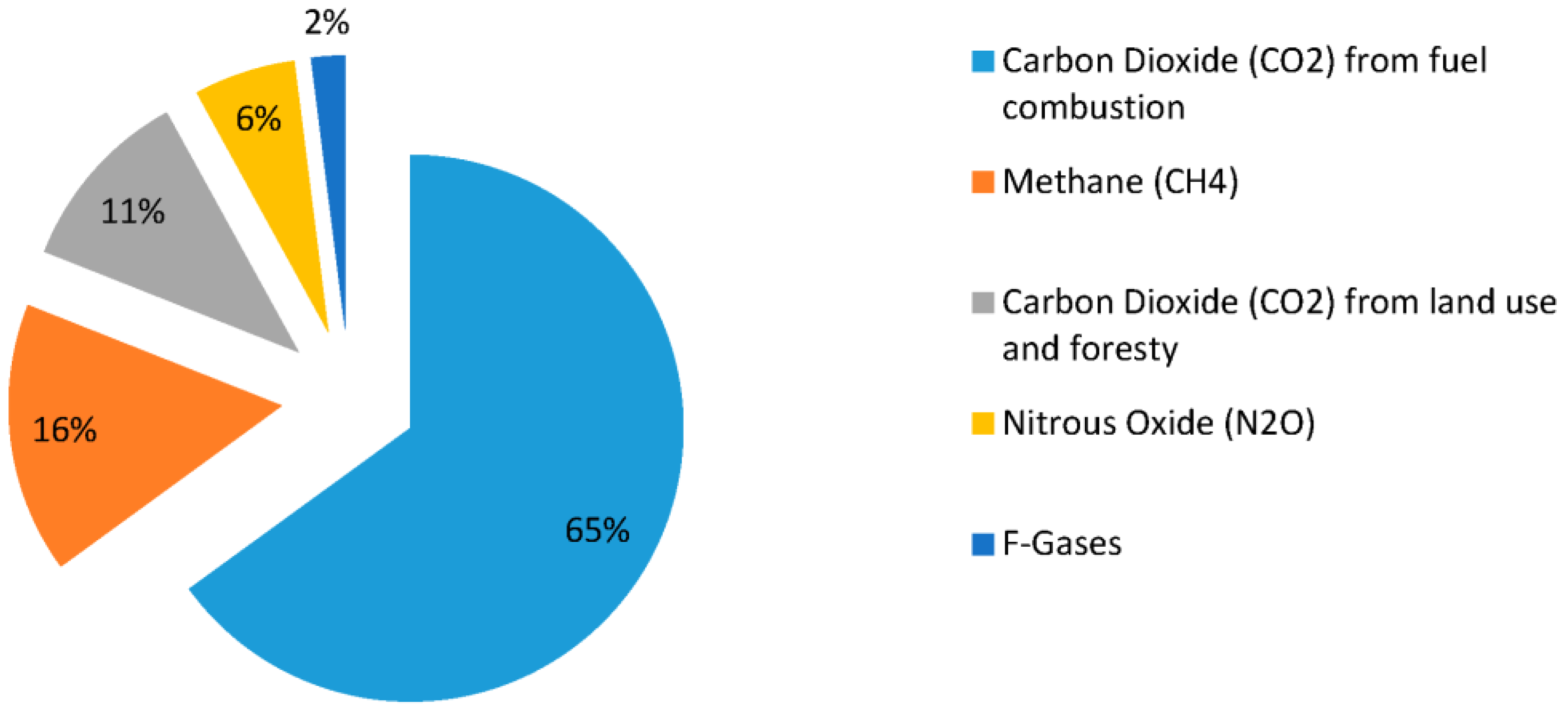
Data on GHG emissions were obtained from the from World Resources Institute (WRI) database (http://datasets.wri.org/dataset/cait-country) and are measured in millions of metric tons of carbon dioxide equivalent (MTCO2e). Unlike most previous studies—which typically use only CO₂ emissions—we use a much broader measure of emissions that includes CO₂, methane (CH₄), nitrous oxide (N₂O), F-gases (e.g., hydrofluorocarbons (HFCs), perfluorocarbons (PFCs), sulfur hexafluoride (SF₆)), as well as GHG equivalents resulting from land-use changes and forestry. This is an important distinction, because while CO₂ makes up the largest share of GHG emissions worldwide, the remaining sources make up a considerable proportion of overall GHG emissions (see Figure 1). Note that the minimum value for GHG emissions in our sample belongs to Malaysia, whose immense forest coverage acts as a carbon sink, absorbing more atmospheric CO₂ annually than the country emits, resulting in negative net emissions [62,63].

GDP data measured in billions of constant 2005 U.S. dollars (USD) were included with the WRI emissions data and converted to billions of constant 2017 USD using the U.S. Bureau of Labor Statistics Consumer Price Index (CPI). The annual growth rate of GDP per capita was easily computed from these data. Also included were data for population and total energy consumption in millions of tons of oil equivalent (Mtoe).

Manufacturing export data were collected from the World Bank’s World Development Indicators database (http://databank.worldbank.org/data/reports.aspx?source=world-development-indicators) and converted to constant 2017 U.S. dollars. Capital stock data were obtained from the International Monetary Fund via the data.world database (https://data.world/imf/investment-and-capital-stock-i) and converted to growth rates. The capital stock for a given country in each year is measured as the total government and private capital stock. A third category, public-private partnership capital stock, is not included due to data limitations. In the countries for which these data were available, this category makes up roughly 1% of the total capital stock on average. Its omission therefore should have very little impact on our estimates. Finally, as noted earlier the HDI data was collected from the United Nations Development Programme. The HDI ranges from 0 to 1, with values closer to 1 indicating a higher overall standard of living along the various component measures.

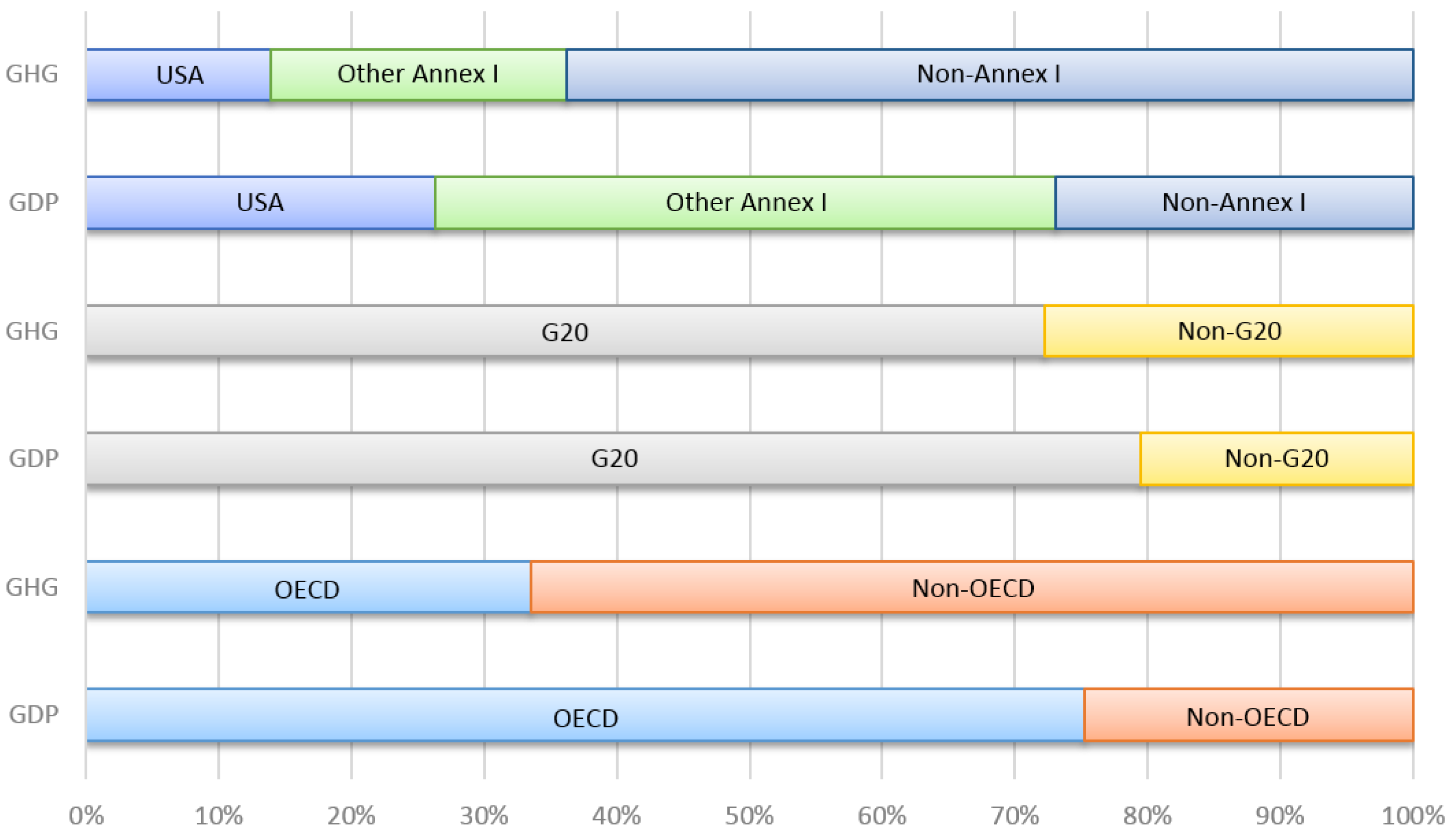
Figure 2 gives a sense of the distribution in 2010 of global GHG emissions relative to the distribution of GDP across the various country groups in Table 1. World GHG emissions totaled 44,237 MTCO2e in 2010, and world GDP was over $66 trillion (2017 USD). Annex I countries accounted for over 36% of GHG emissions, with the U.S. alone generating almost 14%. By contrast, the U.S. accounted for over one-quarter of world GDP, and the remaining Annex I countries another 47%. G20 countries generated over 72% of GHG emissions and accounted for almost 80% of world GDP. OECD countries generated roughly one-third of GHG emissions while accounting for three-quarters of world GDP. The stark contrast in GHG emissions for the G20 versus the OECD is that the G20 includes both China and India, neither of which is a member of the OECD.

One caveat regarding our dataset is that when working with international data of this type, the possibility of measurement error often arises. This is especially so for underdeveloped countries, which often lack the institutions needed for the collection of accurate national-level data like GDP. However, as all our data originate from highly credible sources that have a strong interest in providing the most accurate data possible, we feel safe in assuming measurement error to be minimized.

4. Results

4.1. Preliminary Analysis

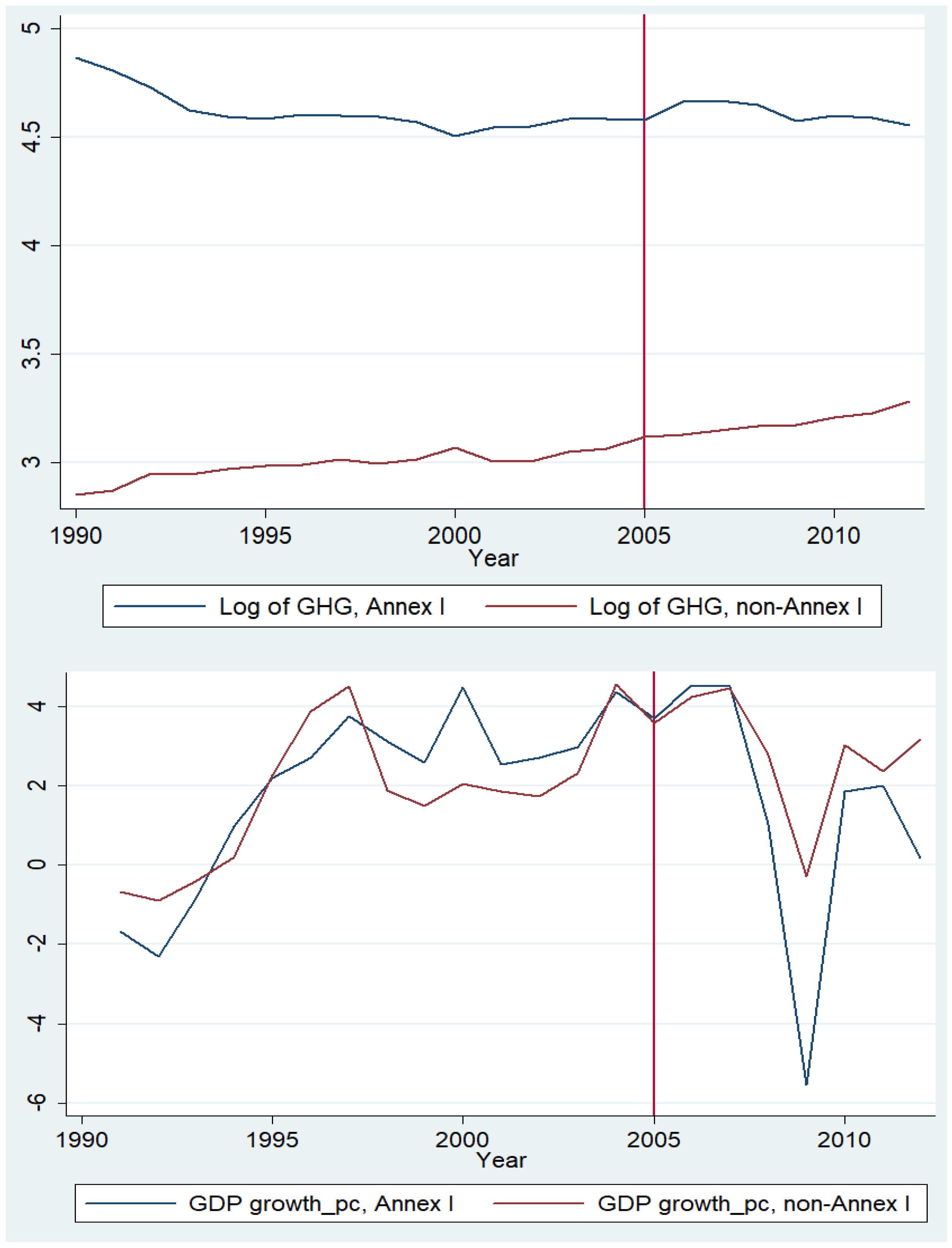
We begin by exploring some basic characteristics of the unconditional data for our two dependent variables, GHG emissions and GDP per capita growth. The top panel of Figure 3 plots the unconditional averages of the (log of) GHG emissions over our sample period for both Annex I and non-Annex I countries, with the year the Kyoto Protocol entered into force (2005) clearly marked. We see that, with the exception of the first 3–4 years of the sample period, GHG emissions have remained fairly steady on average across the Annex I countries, with an upward trend from around 1999–2006 that turned slightly downward thereafter. By contrast, emissions have been consistently increasing over time for non-Annex I countries. To the naked eye, it appears that the growth of emissions across non-Annex I countries may have increased slightly in the post-treatment period.

This visualization of the unconditional data thus yields an important intuition about our results. A negative, statistically significant DiD treatment effect indicates that the Kyoto Protocol—rather than inducing a reduction in GHG emissions by Annex I countries—may have instead successfully prevented the Annex I countries from increasing GHG emissions in the post-treatment period as their non-Annex I counterparts did.

Table 3. t-test of sample means of log(GHG) before and after Kyoto Protocol entered into force, Annex I vs. non-Annex I.

Log(GHG)	Before 2005	After 2005	t-Stat 1	p-Value 2	p-Value 3	p-Value 4
Annex I
# obs.	558	313	-	-	-	-
Mean  (st. err.)	4.615 (0.076)	4.611 (0.098)	0.034	0.514	0.973	0.487
Non-Annex I
# obs.	2055	1135	-	-	-	-
Mean  (st. err.)	2.894 (0.051)	3.180 (0.680)	−2.312	0.010	0.021	0.990

¹ t-stat based on difference in means; Diff = mean (before 2005)–mean(after 2005). ² H_a: $Diff<0$, p-value represents probability $T<t$. ³ H_a: $Diff\ne 0$, p-value represents probability $\left|T\right|\ne \left|t\right|$. ⁴ H_a: $Diff>0$, p-value represents probability $T>t$.

presents a simple t-test of the unconditional means of log(GHG) in the pre- and post-treatment periods for both Annex I and non-Annex I countries. The null hypothesis for this test is that the sub-sample mean is equal across the pre- versus post-treatment periods. Results confirm that the post-treatment mean of log(GHG) is statistically equivalent to the pre-treatment mean for Annex I countries, whereas for non-Annex I countries the post-treatment mean of log(GHG) is significantly higher than the pre-treatment mean.

The lower panel of Figure 3 plots the average GDP per capita growth rates for these two groups. Prior to 2005, both Annex I and non-Annex I countries experienced increasing GDP per capita growth rates over time. After 2005 economic growth declined due to several macroeconomic factors, with the large negative spike in 2009 resulting from the global recession that began with the bursting of the U.S. housing bubble in late 2007 and was then exacerbated by the European debt crisis two years later. It is clear in Figure 3 that the Annex I countries were hit much harder by this negative economic shock, a factor we address in more detail below.

Table 4. t-test of sample means of GDP per capita growth rates before and after Kyoto Protocol entered into force, Annex I vs. non-Annex I.

GDP per Capita Growth	Before 2005	After 2005	t-Stat 1	p-Value 2	p-Value 3	p-Value 4
Annex I
# obs.	542	320	-	-	-	-
Mean  (st. err.)	2.050 (0.191)	1.531 (0.242)	1.675	0.953	0.094	0.047
Non-Annex I
# obs.	1865	1106	-	-	-	-
Mean  (st. err.)	1.801 (0.190)	2.915 (0.171)	−3.976	0.000	0.000	1.000

¹ t-stat based on difference in means; Diff = mean(before 2005)–mean(after 2005). ² H_a: $Diff<0$, p-value represents probability $T<t$. ³ H_a: $Diff\ne 0$, p-value represents probability $\left|T\right|\ne \left|t\right|$. ⁴ H_a: $Diff>0$, p-value represents probability $T>t$.

presents t-tests of the pre- and post-treatment period unconditional means, which indicate that GDP per capita growth rates for Annex I countries were, on average, significantly lower after 2005, whereas growth rates for non-Annex I countries were significantly higher. However, because these are unconditional means, we cannot say with any confidence whether these differences are associated with impacts from the Kyoto Protocol, or from general macroeconomic conditions. To get a better sense of this, we turn to our regression analysis in the next section.

Finally, a key assumption of the DiD methodology is that the variables of interest for the treatment and control groups follow parallel trends leading up to the treatment itself (conditional on other relevant factors). Based on the plots of unconditional trends in Figure 3, satisfaction of the parallel trends assumption appears probable for GDP per capita growth, but less likely for GHG emissions. On the other hand, if the sample interval were restricted to a shorter pre-treatment period, say 1998 forward, the parallel trends assumption appears more reasonable for GHG emissions. In our robustness checks (discussed in Section 4.2.3), we circumvent this issue by eliminating the trend altogether, using multi-year averages for much shorter pre- and post-treatment periods.

4.2. Regression Analysis

Using standard linear regression techniques, we applied Equations (1) and (2) to our data to obtain estimates of the coefficients $\delta$ and $\omega$, the DiD treatment effects for the Kyoto Protocol Annex I designation on GHG emissions and GDP per capita growth, respectively.

Table 5. GHG emissions regressions. Dependent variable: log(GHG).

Variable 1	Whole Sample			G20			OECD
	(1)	(2)	(3)	(4)	(5)	(6)	(7)	(8)	(9)
DiD treatment effect	−0.197 *** (0.040)	−0.064 * (0.033)	−0.030 *** (0.010)	−0.142 (0.069)	0.026 (0.053)	0.007 (0.018)	−0.247 *** (0.059)	−0.172 *** (0.060)	−0.070 ** (0.033)
Log(GDP)	0.302 *** (0.059)	−0.685*** (0.224)	−0.104 ** (0.049)	0.672 *** (0.081)	−0.085 (0.729)	0.163 (0.229)	0.628 *** (0.196)	−0.656 (0.753)	−0.089 (0.300)
Log(GDP) squared		0.037 *** (0.009)	0.007 *** (0.002)		0.011 (0.023)	−0.003 (0.007)		0.043 (0.029)	0.012 (0.010)
Log(energy consumption)		0.538 *** (0.104)	0.150 *** (0.034)		0.749 *** (0.176)	0.223 ** (0.082)		0.690 *** (0.249)	0.223 ** (0.102)
Log(population)		−0.443 ** (0.188)	−0.208 *** (0.061)		−0.344 (0.437)	−0.240 * (0.126)		−0.866 (0.666)	−0.614 * (0.320)
Log(manufacturing exports)		−0.020 (0.012)	−0.002 (0.004)		0.025 (0.051)	0.004 (0.013)		−0.045 (0.084)	−0.036 (0.050)
HDI		0.946 (0.752)	0.335 (0.286)		−0.331 (0.644)	−0.093 (0.162)		1.793 (2.019)	1.025 (1.180)
Lagged dependent variables
L1.Log(GHG)			0.766 *** (0.041)			0.704 *** (0.085)			0.737 *** (0.078)
L2.Log(GHG)			0.003 (0.033)			0.054 (0.060)			−0.034 (0.039)
Number of observations	3847	2306	2152	435	397	365	759	732	673
Number of countries	179	145	144	19	18	18	35	34	34
R-squared	0.272	0.393	0.766	0.767	0.869	0.947	0.200	0.307	0.641

¹ Each model contains country and year fixed effects (not reported). Robust standard errors in parentheses. *** p < 0.01; ** p < 0.05; * p < 0.1.

presents our results for GHG emissions.

Table 6. Growth regressions. Dependent variable: growth rate of GDP per capita.

Variable 1	Whole Sample			G20			OECD
	(1)	(2)	(3)	(4)	(5)	(6)	(7)	(8)	(9)
DiD treatment effect	−1.302 ** (0.527)	−1.729 *** (0.497)	−1.459 *** (0.367)	−1.736 * (0.881)	−2.925 *** (0.774)	−2.489 *** (0.586)	−0.765 (0.507)	−0.692 (0.444)	−0.826 ** (0.366)
Capital stock growth	0.500 *** (0.168)	0.307 *** (0.091)	0.261 *** (0.077)	−0.072 (0.173)	0.503 (0.294)	−0.149 (0.254)	0.170 (0.136)	0.529 *** (0.107)	0.487 *** (0.158)
L1. Capital stock growth		−0.202 ** (0.085)	−0.211 ** (0.081)		−0.869 ** (0.382)	−0.314 (0.188)		−0.581 *** (0.120)	−0.561 *** (0.084)
HDI		7.004 (9.343)	12.534 (8.964)		−6.409 (7.651)	3.187 (6.140)		1.445 (17.911)	2.925 (17.852)
Lagged dependent variables
L1.Log(GHG)			0.174 *** (0.053)			0.264 *** (0.078)			0.251 *** (0.089)
L2.Log(GHG)			0.019 (0.047)			0.165 (0.104)			−0.070 (0.076)
Number of observations	3146	2750	2630	418	378	360	697	644	613
Number of countries	146	145	145	19	18	18	32	31	31
R-squared	0.198	0.136	0.180	0.225	0.338	0.417	0.396	0.505	0.554

¹ Each model contains country and year fixed effects (not reported). Robust standard errors in parentheses. *** p < 0.01; ** p < 0.05; * p < 0.1.

presents our results for GDP per capita growth. We also present in these tables our estimates of the coefficients $\beta$ and $\xi$ on the relevant covariates of each model, but do not report the country or year fixed effects (${\alpha }_i$, ${\gamma }_t$, ${\theta }_i$, ${\tau }_t$). This is common practice. Because a different fixed effect coefficient is estimated for every country and year in the sample, in our model there are 185 countries fixed effects (for the full sample) and 22 years fixed effects.

4.2.1. GHG Emissions

For GHG emissions, we find a negative, statistically significant DiD treatment effect across several different model specifications. We report nine regression models, which can be subdivided into three different groups according to the subsample of countries used. In Models (1)–(3) we use our entire sample of 185 countries. In Models (4)–(6) we use only G20 countries. In Models (7)–(9) we use only OECD countries. For each subsample, we run three different models featuring different sets of explanatory variables.

Models (1), (4) and (7) include estimates for only the DiD treatment and log(GDP), and in each subsample we find a highly significant, negative impact of the Kyoto Protocol Annex I designation on GHG emissions. However, these estimates of the DiD treatment effect are likely to suffer from considerable omitted variable bias, and are thus likely to be higher than the true impact. Models (2), (5) and (8) include our remaining covariates of interest, whereas Models (3), (6) and (9) additionally include two lagged terms of the dependent variable to account for serial correlation in the error structure. Models without the lagged dependent variable terms display moderate serial correlation in the error structure. Including two lag terms successfully eliminates this problem, as indicated by two commonly used test statistics (not reported). However, in dynamic panel models the inclusion of lagged dependent variable terms may lead to biased coefficient estimates when the number of periods (years, in our case) is small. Fortunately, our 22-year sample interval is relatively long, reducing this concern.

As expected, when the additional covariates are included the DiD treatment effect estimate is much lower, but is still statistically significant for the whole sample and for the OECD subsample. For the G20 subsample, the sign of the DiD estimate switches to positive in Models (5) and (6), but the statistical significance disappears. There are likely two reasons for this. First, there are proportionally fewer non-Annex I countries in the G20 subsample than in the whole sample or the OECD subsample. Second, the G20 subsample is the smallest and therefore has the fewest observations over which to estimate the coefficients of interest, which has the effect of increasing the standard errors. For the whole sample and OECD subsample, including the lagged dependent variable terms reduces the magnitude of the DiD treatment effect further, but in each case the effect is still negative and statistically significant, indicating the Kyoto Protocol Annex I designation was effective in limiting emissions increases relative to non-Annex I countries, both at the global level and within the OECD.

Examining some of our other coefficient estimates, not surprisingly total energy consumption is a strong determinant of total GHG emissions. Also, we find little evidence to support the EKC hypothesis with respect to total GHG emissions. The first-order effect of GDP on emissions is positive and statistically significant when the square term is not included. With the square term the sign on the first-order effect flips, and the two GDP terms are only statistically significant when the whole sample of countries is used. The correlation between population and emissions is negative—most likely because more populous countries tend to be poorer and therefore emit less—but the coefficient estimate is statistically significant in only four of the six models in which population is included. Finally, our coefficient estimates on manufacturing exports and on the HDI suggest little that would indicate any systematic relationship between these variables and GHG emissions.

To get a sense of the magnitudes of the DiD treatment effect estimates in Table 5, consider the estimate in Model (9) of −0.07. The counterfactual associated with this estimate is that, all else equal, the Annex I countries of the OECD would have increased annual GHG emissions on average by exp(0.07) = 1.07 MTCO2e in the post-treatment period. For a large country like the U.S. this is clearly a trivial amount. For much smaller countries such as those of the European Union, this represents roughly between a 0.5% and 1% increase in GHG emissions avoided on average in the post-treatment period—still not an impressive result, which calls into question the UNFCCC’s effectiveness in inducing meaningful emissions reductions via such large scale international agreements. To be sure, it may be that the bulk of emissions reductions resulting from current investments and policies had yet to be fully realized in the post-treatment sample period under investigation. However, if the best that can be accomplished is that Annex I countries maintain current GHG emissions levels while non-Annex I countries continue to increase their own emissions, the goal of limiting the rise in global temperatures to 2 °C by 2100 will be difficult to achieve.

4.2.2. GDP Per Capita Growth

That the Kyoto Protocol had a relatively small impact on GHG emissions is particularly troubling when we consider the results of our regressions using GDP per capita growth rates as the dependent variable. Following the Kyoto Protocol entering into force in 2005 Annex I countries appear to have experienced lower GDP per capita growth rates relative to non-Annex I countries. Such a consequence is likely to be politically unpopular, as seen already in the United States. In Table 6, as with our regression models using log(GHG) as the dependent variable, we report nine variations of our growth regression model using the three different subsamples of countries and including different arrangements of explanatory variables and lag terms. Although our regression model does not explain a large share of the variation in GDP per capita growth rates across countries as indicated by the low R-squared statistics, this is not especially surprising; economic growth rates are generally difficult to predict owing to considerable stochasticity. The key result is that in all nine regressions the DiD treatment effect is negative and in seven of nine it is found to be statistically significant at 90 percent confidence or better. This indicates a strong likelihood that the responsibilities attendant upon Kyoto Protocol Annex I countries to curb GHG emissions had the undesirable effect of inhibiting economic growth as well.

As the DiD estimates in Table 6 are expressed in terms of percentage points, Models (1)–(3) suggest that Annex I countries experienced a reduction in annual GDP per capita growth of between roughly 1.3 and 1.7 percentage points on average in the post-treatment period. Within the G20 countries, the impact was more pronounced; our estimates of the DiD treatment effect in this subsample ranges between 1.7 and 2.9 percentage point reduction in GDP per capita growth. This is not surprising, given that G20 countries that are also Annex I countries are among the richest in the world, and therefore shouldered most of the financial burden under the Kyoto Protocol. When the OECD subsample is used, the DiD treatment effect is lower and loses statistical significance in two out of three models. This is perhaps due to the fact that there is greater overlap between the OECD and the Annex I designation, with less variation in GDP per capita growth rates across the subsample. To get an idea of the magnitudes of these differences in terms of dollar amounts, the average GDP per capita of Annex I countries post-2005 was roughly $36,700 (constant 2017 USD); an average loss of 1.7 percentage points translates to over $600 per year in lost income per capita growth, a considerable amount when aggregated to the total population.

4.2.3. Robustness Checks

In econometric analyses, it is often desirable to check whether the results of interest—in our case the effect of the Annex I designation on countries’ GHG emissions and GDP per capita growth rates—are robust to alternative regression specifications. This serves to reduce concerns that the desired results are potentially spurious. We present four alternative specification is

Table 7. GHG emissions robustness check: Pre- and Post-treatment averages.

Variable 1	Whole Sample		G20		OECD
	(1)	(2)	(3)	(4)	(5)	(6)
DiD treatment effect	−0.143 *** (0.033)	−0.106 ** (0.041)	−0.165 *** (0.033)	−0.047 (0.051)	−0.173 *** (0.040)	−0.174 ** (0.081)
Log(GDP)	0.433 *** (0.066)	−0.806 *** (0.246)	0.665 *** (0.078)	−0.646 (0.862)	0.575 *** (0.132)	−0.795 (0.942)
Log(GDP) squared		0.046 *** (0.011)		0.025 (0.028)		0.053 (0.040)
Log(energy cons.)		0.535 *** (0.155)		1.036 *** (0.203)		0.494 * (0.289)
Log(population)		0.044 (0.109)		0.095 (0.310)		−0.440 (0.627)
Log(manuf. exp.)		−0.006 (0.037)		−0.150 (0.096)		−0.163 (0.116)
HDI		−0.735 (0.813)		1.481 (1.106)		3.386 * (1.710)
# observations	222	222	36	36	66	66
# countries	111	111	18	18	33	33
R-squared	0.378	0.572	0.834	0.906	0.224	0.355

¹ Each model includes country fixed effects (not reported). Robust standard errors in parentheses. *** p < 0.01; ** p < 0.05; * p < 0.1.

,

Table 8. GHG emissions robustness check: Pre- and Post-treatment averages, U.S. omitted.

Variable 1	Whole Sample		G20		OECD
	(1)	(2)	(3)	(4)	(5)	(6)
DiD treatment effect	−0.144 *** (0.033)	−0.104 ** (0.041)	−0.163 *** (0.036)	−0.047 (0.052)	−0.174 *** (0.042)	−0.172 * (0.085)
Log(GDP)	0.433 *** (0.066)	−0.814 *** (0.248)	0.665 *** (0.078)	−0.720 (1.033)	0.576 *** (0.132)	−0.863 (1.007)
Log(GDP) squared		0.047 *** (0.011)		0.028 (0.035)		0.057 (0.046)
Log(energy cons.)		0.533 *** (0.155)		1.023 *** (0.223)		0.499 * (0.286)
Log(population)		0.046 (0.109)		0.122 (0.365)		−0.459 (0.656)
Log(manuf. exp.)		−0.006 (0.037)		−0.149 (0.099)		−0.167 (0.122)
HDI		−0.739 (0.812)		1.428 (1.176)		3.331 * (1.803)
# observations	220	220	34	34	64	64
# countries	110	110	17	17	32	32
R-squared	0.378	0.572	0.834	0.906	0.223	0.355

¹ Each model includes country fixed effects (not reported). Robust standard errors in parentheses. *** p < 0.01; ** p < 0.05; * p < 0.1.

,

Table 9. GDP per capita growth robustness check: Pre- and Post-treatment averages.

Variable 1	Whole Sample		G20		OECD
	(1)	(2)	(3)	(4)	(5)	(6)
DiD treatment effect	−3.053 *** (0.388)	−3.668 *** (0.444)	−1.627 ** (0.735)	−3.522 *** (1.073)	−2.334 *** (0.511)	−2.720 *** (0.632)
Capital stock growth	0.029 (0.111)	−0.077 (0.109)	0.539 * (0.273)	0.056 (0.290)	0.627 * (0.331)	0.614 * (0.333)
HDI		12.532 ** (5.893)		42.349 * (21.298)		9.226 (18.715)
# observations	198	198	36	36	62	62
# countries	99	99	18	18	31	31
R-squared	0.262	0.291	0.338	0.521	0.678	0.680

¹ Each model includes country fixed effects (not reported). Robust standard errors in parentheses. *** p < 0.01; ** p < 0.05; * p < 0.1.

and

Table 10. GDP per capita growth robustness check: Pre- and Post-treatment averages, 2009 omitted.

Variable 1	Whole Sample		G20		OECD
	(1)	(2)	(3)	(4)	(5)	(6)
DiD treatment effect	−1.582 *** (0.380)	−2.561 *** (0.443)	−0.250 (0.832)	−2.517 * (1.216)	−0.916 * (0.533)	−2.383 *** (0.603)
Capital stock growth	0.223 * (0.132)	0.054 (0.127)	0.716 ** (0.281)	0.133 (0.296)	0.764 ** (0.309)	0.733 ** (0.303)
HDI		18.248 *** (5.971)		46.967 * (24.228)		34.207 ** (15.529)
# observations	198	198	36	36	62	62
# countries	99	99	18	18	31	31
R-squared	0.131	0.197	0.289	0.490	0.513	0.569

¹ Each model includes country fixed effects (not reported). Robust standard errors in parentheses. *** p < 0.01; ** p < 0.05; * p < 0.1.

.

In DiD models, one such concern is raised by the possibility that the DiD treatment effect is transient. In other words, the statistically significant result may be driven by impacts realized immediately after the treatment occurs, but that then fade as time passes. Another concern is that the parallel trends assumption may be violated. To avoid these issues, a common approach is to use multi-period averages rather than annual data, and omit the data pertaining to a sufficiently large window around the treatment itself [64]. To do this, we first define the ‘treatment period’ as the five-year period from 2003–2007; these observations are dropped from the data. We then define the five years prior, 1998–2002, as the pre-treatment period and take averages of all relevant variables. Last, we define the five-year period 2008–2012 as the post-treatment period and take averages for this interval. Defining these five-year symmetric intervals around the treatment period serves to eliminate the possibility that our results are being driven by differences early in the sample interval (i.e., prior to 1998), which may no longer be relevant for reasons undetectable with our data. This specification has the additional benefit of minimizing the effects of country-specific business cycles on the dependent variables, which is particularly important given the major global recession that strongly impacted Annex I countries in 2009.

For each subsample, we utilize only those countries that have complete data series for all variables in the five-year pre- and post-treatment intervals, such that the panel is perfectly balanced and contains exactly two observations per country—one five-year average for the pre-treatment period and one for the post-treatment period. As all variables are expressed as averages, lagged terms and year fixed effects are no longer sensible and are therefore not included.

Results for GHG emissions are presented in Table 7. The estimated DiD treatment effects are generally consistent with those of our main specifications in Table 5. One difference is that the magnitude of the estimated DiD treatment effect is more consistent across the different models in Table 7 than in Table 5. Excluding Model (4), in which the coefficient is not statistically significant, estimates range from −0.106 in Model (2) to −0.174 in Model (6), which correspond to avoided emissions increases by the Annex I countries of 1.11–1.19 million MTCO2e annually in the post-treatment period.

One might wonder whether these modest emissions reduction estimates reflect the fact that the U.S., by far the largest GHG emitter among the Annex I countries, never ratified the KP nor implemented its requirements in a significant way. Dropping the U.S. from the sample might therefore yield a stronger result for the DiD treatment effect. To the contrary, we find only negligible differences in the point estimates when the U.S. is excluded from the sample (see Table 8), indicating that our results are not influenced significantly by the U.S. as the sole non-ratifying Annex I country. The DiD treatment effect of the KP on Annex I countries’ GHG emissions is small but statistically significant across a number of different empirical specifications and country samples.

Results for GDP per capita growth are presented in Table 9. Here, our estimates of the DiD treatment effect are of a generally greater magnitude than their counterparts in Table 6. This is partly due to the exclusion of observations early in the sample period (i.e., 1990–1997) when growth rates were much lower (see Figure 3). However, it is still quite possible that the 2009 recession is pulling average growth rates down in the post-treatment period to a degree that the estimated DiD treatment effect in Table 9 overstates the true average effect. To see this, in Table 10 we repeat the regressions in Table 9, except the post-treatment period average is computed after dropping 2009; in other words, the post-treatment averages are now computed over years 2008, 2010, 2011 and 2012. As expected, the magnitudes of the estimates for the DiD treatment effect are generally considerably lower than their counterparts in Table 9, and we lose statistical significance when the G20 subsample is used. However, there is still compelling evidence in the full sample and the OECD subsample regressions to support the hypothesis that Annex I countries experienced lower economic growth relative to non-Annex I countries after the Kyoto Protocol entered into force.

5. Discussion

Although we find statistically significant results with respect to both GHG emissions and GDP per capita growth rates that are generally robust to a variety of empirical specifications and country groupings, a number of questions remain. In this section, we briefly discuss some of these questions, which also provide opportunities for continuing research on the impacts of international climate agreements under the UNFCCC.

For one, the R-squared values in several of our regressions are relatively low, meaning our covariates and fixed effects do not explain as much of the total variation in GHG emissions and GDP growth rates—both across countries and over time—as we would like. On the one hand, this is not especially surprising and does not undermine the overall inference of our DiD estimates with respect to the KP Annex I designation. On the other hand, there are any number of potentially important explanatory variables that are not included in our regressions, which leaves open the possibility of omitted variable bias with regard to the point estimates themselves. For GHG emissions there is likely to be within-country variation over time in such things as renewable energy support policies—e.g., feed-in tariffs and renewable portfolio standards—that would influence investments in clean energy technologies [65,66,67]. Many countries had such policies in place—and as a result began reducing GHG emissions—long before the KP entered into force in 2005. The variation in GDP per capita growth is arguably more complex and idiosyncratic. Researchers have found impacts—in some cases on GDP growth and in others on GDP per capita growth—related to such wide-ranging factors as natural resource dependence (i.e., “Dutch disease”) (see [68] for a comprehensive review), oil price shocks [69], mobile phone usage rates [70], public sector corruption [71,72,73], human capital development [74], and foreign direct investment [75]. Controlling for such impacts in our analysis is an important next step in continuing research, and will help improve the explanatory power of our regression models and the precision of our point estimates.

With respect to our regressions using GDP per capita growth rates as the dependent variable, one might assert that our key results could be interpreted as illustrating the widely known convergence hypothesis (see [76] for a survey of the literature). This seems unlikely. The convergence hypothesis, simply stated, is that GDP per capita should grow faster in poorer countries than in richer countries. While it is true that the KP Annex I countries tend to be richer than the non-Annex I countries, the fact that our key result is robust to restricting the sample to only the G20 countries—which tend to be among the richest in the world—seems inconsistent with the convergence hypothesis. Second, GDP per capita growth rates were, on average, very similar for Annex I versus non-Annex I countries prior to 2005. Third, the convergence hypothesis states that over time, as GDP per capita converges between rich and poor countries, so will the growth rates. This implies that growth rates should be higher for poorer countries relative to richer countries earlier in the sample, which is the opposite of what our DiD estimates indicate.

Other possibilities for continuing research are to experiment with (i) alternative country groupings aside from just the G20 and OECD subsamples; or (ii) more complex empirical specifications. The motivation for testing for the DiD treatment within just the G20 and OECD was straightforward; these country groupings contain some of the world’s largest economies in terms of GDP and are among the largest emitters of GHG’s (see Figure 2). Might our key results hold up if we restricted the sample to only European Union members, only Asian-Pacific countries, or only NATO countries, etc.? Because of the strong economic ties resulting from free trade agreements and other shared international institutions, we should expect to find differential impacts that are strongly dependent on the subsample of countries used. Regarding our empirical specification, in this paper we have treated the impacts of the KP Annex I designation on GHG emissions and GDP per capita growth separately. It is quite possible, however, that these effects are not entirely independent of one another. It would be of interest to utilize a seemingly unrelated regressions model, for example, in which the two regression equations are estimated simultaneously as a system to control for the possibility that the error terms are correlated across equations [77].

6. Conclusions

International climate agreements such as the Kyoto Protocol of 1997 and, more recently, the Paris Climate Agreement are fragile because, at a national level, political constituencies’ value systems may conflict with the goal of reducing greenhouse gas (GHG) emissions to sustainable levels. This conflict was on display in 2017 when the United States withdrew from the Paris Climate Agreement under President Trump, to the consternation of the rest of the international community.

Proponents of such international agreements cite climate change as the most pressing challenge of our time, and rightly contend that international cooperation in reducing GHG emissions will play an essential role in addressing this challenge. Political opponents to these agreements argue that the disproportionate requirements on developed nations to shoulder the financial burden will inhibit their economic growth. We find empirical evidence that both arguments are likely to be correct.

Using standard regression techniques to analyze a multi-country dataset of GHG emissions, GDP per capita growth, and other relevant factors over a period spanning 22 years, we estimate that ‘Annex I’ countries under the Kyoto Protocol reduced GHG emissions on average by roughly 1 million metric tons of CO₂ equivalent after 2005 (the year the Kyoto Protocol entered into force), relative to non-Annex I countries. Our estimates also reveal that these countries experienced a reduction in GDP per capita growth rates of around 1–2 percentage points after 2005 relative to non-Annex I countries, a result that is robust to a number of different empirical specifications.

The trade-off between reduced GHG emissions and greater economic growth is not an illusion; the former incurs real costs that appear significantly to inhibit the latter. It is therefore incumbent upon international bodies such as the United Nations Framework Convention on Climate Change (UNFCCC)—and other, regional coalitions—to acknowledge this trade-off directly and develop ways to mitigate the impacts on economic growth of taking a leadership role in crucial international climate agreements. Otherwise, the rejection of these agreements by political constituencies who value short-term economic growth over long-term climate benefits will present a constant threat to their viability and success.

References

- Rice, D. The U.S. Is Now the Only Country Not Part of Paris Climate Agreement after Syria Signs On. USA Today, 7 November 2017. Available online: https://www.usatoday.com/story/weather/2017/11/07/u-s-now-only-country-not-part-paris-climate-agreement-after-syria-signs/839909001/ (accessed on 19 December 2017).
- Ringius, L.; Torvanger, A.; Underdal, A. Burden Sharing and Fairness Principles in International Climate Policy. Int. Environ. Agreem. Politics Law Econ. 2002, 2, 1–22. [Google Scholar] [CrossRef]
- Finus, M.; Altamirano-Cabrera, J.C.; van Ierland, E.C. The effect of membership rules and voting schemes on the success of international climate agreements. Public Choice 2005, 125, 95–127. [Google Scholar] [CrossRef]
- Altamirano-Cabrera, J.C.; Finus, M. Permit Trading and Stability of International Climate Agreements. J. Appl. Econ. 2006, 9, 19–47. [Google Scholar]
- Weikard, H.P.; Finus, M.; Altamirano-Cabrera, J.C. The impact of surplus sharing on the stability of international climate agreements. Oxf. Econ. Pap. 2006, 58, 209–232. [Google Scholar] [CrossRef]
- Bechtel, M.M.; Scheve, K.F. Mass support for global climate agreements depends on institutional design. Proc. Natl. Acad. Sci. USA 2013, 110, 13763–13768. [Google Scholar] [CrossRef] [PubMed]
- Bosetti, V.; Carraro, C.; De Cian, E.; Massetti, E.; Tavoni, M. Incentives and stability of international climate coalitions: An integrated assessment. Energy Policy 2013, 55, 44–56. [Google Scholar] [CrossRef] [Green Version]
- Cherry, T.L.; Hovi, J.; McEvoy, D. (Eds.) Toward a New Climate Agreement: Conflict, Resolution, and Governance; Routledge Books: London, UK, 2014; ISBN 0415643791. [Google Scholar]
- Huang, W.M.; Lee, G.W.M.; Wu, C.C. GHG emissions, GDP growth and the Kyoto Protocol: A revisit of the Environmental Kuznets Curve hypothesis. Energy Policy 2008, 36, 239–247. [Google Scholar] [CrossRef]
- Achiele, R.; Felbermayr, G. Kyoto and the carbon footprint of nations. J. Environ. Econ. Manag. 2012, 63, 336–354. [Google Scholar] [CrossRef]
- Gupta, J. A history of international climate change policy. WIREs Clim. Chang. 2010, 1, 636–653. [Google Scholar] [CrossRef]
- United Nations Framework Convention on Climate Change. Kyoto Protocol to the United Nations Framework Convention on Climate Change. 1998. Available online: http://unfccc.int/resource/docs/convkp/kpeng.pdf (accessed on 14 November 2017).
- Barrett, S.; Stavins, R. Increasing Participation and Compliance in International Climate Change Agreements. Int. Environ. Agreem. Politics Law Econ. 2003, 3, 349–376. [Google Scholar] [CrossRef]
- Barrett, S. Political Economy of the Kyoto Protocol. Oxf. Rev. Econ. Policy 1998, 14, 20–39. [Google Scholar] [CrossRef]
- Nordhaus, W.B.; Boyer, J.G. Requiem for Kyoto: An Economic Analysis of the Kyoto Protocol. Energy J. 1999, 20, 93–130. [Google Scholar] [CrossRef]
- United Nations Framework Convention on Climate Change. Copenhagen Accord. 2009. Available online: http://unfccc.int/resource/docs/2009/cop15/eng/l07.pdf (accessed on 14 November 2017).
- Dimitrov, R.S. Inside Copenhagen: The State of Climate Governance. Glob. Environ. Politics 2010, 10, 18–24. [Google Scholar] [CrossRef]
- Nordhaus, W.B. Economic aspects of global warming in post-Copenhagen environment. Proc. Natl. Acad. Sci. USA 2010, 107, 11721–11726. [Google Scholar] [CrossRef] [PubMed]
- Falkner, R.; Stephan, H.; Vogler, J. International Climate Policy after Copenhagen: Towards a ‘Building Blocks’ Approach. Glob. Policy 2010, 1, 252–262. [Google Scholar] [CrossRef] [Green Version]
- United Nations Framework Convention on Climate Change. Paris Agreement. 2009. Available online: http://unfccc.int/files/essential_background/convention/application/pdf/english_paris_agreement.pdf (accessed on 14 November 2017).
- Center for Climate and Energy Solutions. Essential Elements of a Paris Climate Agreement. December 2015. Available online: https://www.c2es.org/site/assets/uploads/2015/12/essential-elements-paris-climate-agreement.pdf (accessed on 1 September 2017).
- U.S. Environmental Protection Agency. Available online: https://www.epa.gov/ghgemissions/global-greenhouse-gas-emissions-data (accessed on 26 September 2017).
- Council on Foreign Relations. The Consequences of Leaving the Paris Agreement. Available online: https://www.cfr.org/backgrounder/consequences-leaving-paris-agreement (accessed on 1 September 2017).
- Sanger, D.E. Bush Will Continue to Oppose Kyoto Pact on Global Warming. The New York Times, 12 June 2001. Available online: http://www.nytimes.com/2001/06/12/world/bush-will-continue-to-oppose-kyoto-pact-on-global-warming.html (accessed on 10 January 2018).
- Coon, C. Why President Bush Is Right to Abandon the Kyoto Protocol. The Heritage Foundation, 11 May 2001. Available online: http://www.heritage.org/environment/report/why-president-bush-right-abandon-the-kyoto-protocol (accessed on 10 January 2018).
- Dayaratna, K.; Loris, N.; Kreutzer, D. Consequences of Paris Protocol: Devastating Economic Costs, Essentially Zero Environmental Benefits. The Heritage Foundation, 13 April 2016. Available online: http://www.heritage.org/environment/report/consequences-paris-protocol-devastating-economic-costs-essentially-zero (accessed on 10 January 2018).
- Volcovici, V.U.S. Submits Formal Notice of Withdrawal from Paris Climate Pact. Reuters, 4 August 2017. Available online: https://www.reuters.com/article/us-un-climate-usa-paris/u-s-submits-formal-notice-of-withdrawal-from-paris-climate-pact-idUSKBN1AK2FM (accessed on 10 January 2018).
- Schipani, V.; Kiely, E.; Robertson, L. Fact-Checking Trump’s Speech on Paris Climate Agreement. USA Today, 2 June 2017. Available online: https://www.usatoday.com/story/news/politics/2017/06/02/fact-checking-trump-speech-paris-climate-agreement/102399674/ (accessed on 10 January 2018).
- Donald Trump’s Withdrawal from the Paris Agreement Is Unpopular with Voters. The Economist, 5 June 2017. Available online: https://www.economist.com/blogs/graphicdetail/2017/06/daily-chart-1 (accessed on 10 January 2018).
- Bodansky, D. The Paris Climate Change Agreement: A New Hope? Am. J. Int. Law 2016, 110, 288–319. [Google Scholar] [CrossRef]
- De Coninck, H.; Fischer, C.; Newell, R.G.; Ueno, T. International technology-oriented agreements to address climate change. Energy Policy 2008, 36, 335–356. [Google Scholar] [CrossRef]
- Nordhaus, W.B. After Kyoto: Mechanisms to Control Global Warming. Am. Econ. Rev. 2006, 96, 31–34. [Google Scholar] [CrossRef]
- Arrow, K.; Bolin, B.; Costanza, R.; Dasgupta, P.; Folke, C.; Holling, C.S.; Jansson, B.O.; Levin, S.; Mäler, K.G.; Perrings, C.; et al. Economic Growth, Carrying Capacity, and the Environment. Ecol. Econ. 1995, 15, 91–95. [Google Scholar] [CrossRef]
- Copeland, B.R.; Taylor, M.S. Trade, Growth, and the Environment. J. Econ. Lit. 2004, 42, 7–71. [Google Scholar] [CrossRef]
- Jalil, A.; Mahmoud, S.F. Environmental Kuznets curve for CO2: A cointegration analysis for China. Energy Policy 2009, 37, 5167–5172. [Google Scholar] [CrossRef]
- Zhang, X.P.; Cheng, X.M. Energy consumption, carbon emissions, and economic growth in China. Ecol. Econ. 2009, 68, 2706–2712. [Google Scholar] [CrossRef]
- Zhang, Y.J. The impact of financial development on carbon emissions: An empirical analysis in China. Energy Policy 2011, 39, 2197–2203. [Google Scholar] [CrossRef]
- Yang, L.; Yuan, S.; Sun, L. The Relationships between Economic Growth and Environmental Pollution Based on Time Series Data: An Empirical Study of Zhejiang Province. J. Camb. Stud. 2012, 7, 33–42. [Google Scholar]
- Li, H.; Li, B.; Lu, H. Carbon Dioxide Emissions, Economic Growth, and Selected Types of Fossil Energy Consumption in China: Empirical Evidence from 1965 to 2015. Sustainability 2017, 9, 697. [Google Scholar]
- Jayanthakumaran, K.; Verma, R.; Liu, Y. CO2 emissions, energy consumption, trade and income: A comparative analysis of China and India. Energy Policy 2012, 42, 450–460. [Google Scholar] [CrossRef]
- Friedl, B.; Getzner, M. Determinants of CO2 emissions in a small open economy. Ecol. Econ. 2003, 45, 133–148. [Google Scholar] [CrossRef]
- Benavides, M.; Ovalle, K.; Torres, C.; Vinces, T. Economic Growth, Renewable Energy and Methane Emissions: Is there an Environmental Kuznets Curve in Austria? Int. J. Energy Econ. Policy 2017, 7, 259–267. [Google Scholar]
- Zambrano-Monserrate, M.A.; Troccoly-Quiroz, A.; Pacheco-Borja, M.J. Testing the Environmental Kuznets Curve Hypothesis in Iceland: 1960–2010. Rev. Econ. Rosario 2016, 19, 5–28. [Google Scholar] [CrossRef]
- Palamalai, S.; Ravindra, I.S.; Prakasam, K. Relationship between energy consumption, CO2 emissions, economic growth and trade in India. J. Econ. Financ. Stud. 2015, 3, 1–17. [Google Scholar] [CrossRef]
- Hossain, M.S. Panel estimation for CO2 emissions, energy consumption, economic growth, trade openness and urbanization of newly industrialized countries. Energy Policy 2012, 39, 6991–6999. [Google Scholar] [CrossRef]
- Ang, J.B. Economic development, pollutant emissions and energy consumption in Malaysia. J. Policy Model. 2008, 30, 271–278. [Google Scholar] [CrossRef]
- Saboori, B.; Sulaiman, J.; Mohd, S. Economic growth and CO2 emissions in Malaysia: A cointegration analysis of the Environmental Kuznets Curve. Energy Policy 2012, 51, 184–191. [Google Scholar] [CrossRef]
- Preap, S. The impact of urbanization and energy consumption on CO2 emission in Thailand. Empir. Econom. Quant. Econ. Lett. 2015, 4, 47–56. [Google Scholar]
- Halicioglu, F. An econometric study of CO2 emissions, energy consumption, income and foreign trade in Turkey. Energy Policy 2009, 37, 1156–1164. [Google Scholar] [CrossRef] [Green Version]
- Soytas, U.; Sari, R. Energy consumption, economic growth, and carbon emissions: Challenges faced by an EU candidate member. Ecol. Econ. 2007, 68, 1667–1675. [Google Scholar] [CrossRef]
- Ozturk, I.; Acaravci, A. CO2 emissions, energy consumption and economic growth in Turkey. Renew. Sustain. Energy Rev. 2010, 14, 3220–3225. [Google Scholar] [CrossRef]
- Dogan, E.; Turkekul, B. CO2 emissions, real output, energy consumption, trade, urbanization and financial development: Testing the EKC hypothesis for the USA. Environ. Sci. Pollut. Res. 2016, 23, 1203–1213. [Google Scholar] [CrossRef] [PubMed]
- Arouri, M.E.H.; Youssef, A.B.; M’henni, H.; Rault, C. Energy Consumption, Economic Growth and CO2 Emissions in Middle East and North African Countries. Discussion Paper Series. Forschungsinstitut zur Zukunft der Arbeit, No. 6412. 2012. Available online: http://ftp.iza.org/dp6412.pdf (accessed on 1 November 2017).
- Omri, A. CO2 emissions, energy consumption and economic growth nexus in MENA countries: Evidence from simultaneous equations models. Energy Econ. 2013, 40, 657–664. [Google Scholar] [CrossRef]
- Zhu, H.; Duan, L.; Guo, Y.; Yu, K. The effects of FDI, economic growth and energy consumption on carbon emissions in ASEAN-5: Evidence from panel quantile regression. Econ. Model. 2016, 58, 237–248. [Google Scholar] [CrossRef]
- Kasman, A.; Duman, Y.S. CO2 emissions, economic growth, energy consumption, trade and urbanization in new EU member and candidate countries: A panel data analysis. Econ. Model. 2015, 44, 97–103. [Google Scholar] [CrossRef]
- Angrist, J.D.; Pischke, J.S. Mostly Harmless Econometrics: An Empiricist’s Companion; Princeton University Press: Princeton, NJ, USA, 2009; ISBN 0691120358. [Google Scholar]
- Fredriksson, P.G.; Neumayer, E. Corruption and Climate Change Policies: Do the Bad Old Days Matter? Environ. Resour. Econ. 2014, 63, 451–469. [Google Scholar] [CrossRef] [Green Version]
- United Nations Development Programme. Available online: http://hdr.undp.org/en/content/human-development-index-hdi (accessed on 14 November 2017).
- Nickell, S. Biases in Dynamic Models with Fixed Effects. Econometrica 1981, 49, 1417–1426. [Google Scholar] [CrossRef]
- Levine, R.; Renelt, D. A Sensitivity Analysis of Cross-Country Growth Regressions. Am. Econ. Rev. 1992, 82, 942–963. [Google Scholar]
- Watson, R.T.; Noble, I.R.; Bolin, B.; Ravindranath, N.H.; Verardo, D.J.; Dokken, D.J. Land Use, Land-Use Change and Forestry. A Special Report of the Intergovernmental Panel on Climate Change (IPCC). 2000. Available online: http://98.131.92.124/sites/default/files/2000%20Watson%20IPCC.pdf (accessed on 10 January 2018).
- Low Carbon Society: Malaysia 2030. Available online: http://2050.nies.go.jp/report/file/lcs_asia/Malaysia.pdf (accessed on 10 January 2018).
- Bertrand, M.; Duflo, E.; Mullainathan, S. How Much Should We Trust Differences-In-Differences Estimates? Q. J. Econ. 2004, 119, 249–275. [Google Scholar] [CrossRef]
- Mendonça, M.; Jacobs, D.; Sovacool, B. Powering the Green Economy: The Feed-In Tariff Handbook; Earthscan: London, UK, 2010; ISBN 1844078582. [Google Scholar]
- Wiser, R.; Porter, K.; Grace, R. Evaluating Experience with Renewables Portfolio Standards in the United States. Mitig. Adapt. Strateg. Glob. Chang. 2005, 10, 237–263. [Google Scholar] [CrossRef]
- Johnson, E.P.; Oliver, M.E. Renewable Energy Support Policies and Wholesale Electricity Price Risk: A Stochastic Merit-Order Effect? Manuscript in Preparation.
- Deacon, R.T. The Political Economy of the Resource Curse: A Survey of Theory and Evidence. Found. Trends Microecon. 2011, 7, 111–208. [Google Scholar] [CrossRef]
- Jiménez-Rodríguez, R.; Sánchez, M. Oil price shocks and real GDP growth: Empirical evidence for some OECD countries. Appl. Econ. 2005, 37, 201–228. [Google Scholar] [CrossRef]
- Gruber, H.; Koutroumpis, P.; Mayer, T.; Nocke, V. Mobile telecommunications and the impact on economic development. Econ. Policy 2011, 26, 389–426. [Google Scholar] [CrossRef]
- Mauro, P. Corruption and Growth. Q. J. Econ. 1995, 110, 681–712. [Google Scholar] [CrossRef]
- Mo, P.H. Corruption and Economic Growth. J. Comp. Econ. 2001, 29, 66–79. [Google Scholar] [CrossRef]
- Aidt, T.; Dutta, J.; Sena, V. Governance regimes, corruption and growth: Theory and evidence. J. Comp. Econ. 2008, 36, 195–220. [Google Scholar] [CrossRef]
- Benhabib, J.; Speigel, M. The role of human capital in economic development: Evidence from aggregate cross-country data. J. Monetary Econ. 1994, 34, 143–173. [Google Scholar] [CrossRef]
- Borensztein, E.; De Gregorio, J.; Lee, J.W. How does foreign direct investment affect economic growth? J. Int. Econ. 1998, 45, 115–135. [Google Scholar] [CrossRef]
- De la Fuente, A. The empirics of growth and convergence: A selective review. J. Econ. Dyn. Control 1997, 21, 23–73. [Google Scholar] [CrossRef]
- Moon, H.R.; Perron, B. Seemingly unrelated regressions. New Palgrave Dict. Econ. 2006, pp. 1–9. Available online: http://mapageweb.umontreal.ca/perrob/palgrave.pdf (accessed on 28 January 2018).
Figure 1.
Global greenhouse gas (GHG) emissions by source, 2010 (Source: U.S. Environmental Protection Agency).
Figure 2.
GHG emissions and GDP, percentages of 2010 world totals for country groups.
Figure 3.
Annex I vs. non-Annex I averages, 1990–2012: (top) log(GHG); (bottom) GDP per capita growth rates.