Comparing the Applicability of Commonly Used Hydrological Ecosystem Services Models for Integrated Decision-Support


1
Section of Engineering Hydrology and Water Management, Technische Universität Darmstadt, 64287 Darmstadt, Germany
2
Institute of Applied Geosciences, Technische Universität Darmstadt, 64287 Darmstadt, Germany
*
Author to whom correspondence should be addressed.
Sustainability 2018, 10(2), 346; https://doi.org/10.3390/su10020346
Submission received: 30 November 2017
/
Revised: 23 January 2018
/
Accepted: 24 January 2018
/
Published: 29 January 2018
(This article belongs to the Special Issue Sustainable River Basin Management)
Abstract
:Different simulation models are used in science and practice in order to incorporate hydrological ecosystem services in decision-making processes. This contribution compares three simulation models, the Soil and Water Assessment Tool, a traditional hydrological model and two ecosystem services models, the Integrated Valuation of Ecosystem Services and Trade-offs model and the Resource Investment Optimization System model. The three models are compared on a theoretical and conceptual basis as well in a comparative case study application. The application of the models to a study area in Nicaragua reveals that a practical benefit to apply these models for different questions in decision-making generally exists. However, modelling of hydrological ecosystem services is associated with a high application effort and requires input data that may not always be available. The degree of detail in temporal and spatial variability in ecosystem service provision is higher when using the Soil and Water Assessment Tool compared to the two ecosystem service models. In contrast, the ecosystem service models have lower requirements on input data and process knowledge. A relationship between service provision and beneficiaries is readily produced and can be visualized as a model output. The visualization is especially useful for a practical decision-making context.
1. Introduction
Over the past millennia mankind has severely changed the global environment [1] and the provision of ecosystem services, the benefits that societies receive from nature, are in a severe decline [2]. To address the continuous degradation of the natural environment and related ecosystem services as well as to guide decisions on the use of the natural environment, tools for the assessment, quantification and valuation of ecosystem services (ES) are being developed. The number of these tools is increasing rapidly. Especially for water management, modelling of hydrological ecosystem services (HES) is becoming increasingly important [3]. Hydrological ecosystem services are defined here as proposed by Brauman et al. [4]: “Hydrologic services encompass the benefits to people produced by terrestrial ecosystem effects on freshwater.” Hydrologic services are organized by Brauman et al. (2007) into five broad categories: improvement of extractive water supply, improvement of in-stream water supply, water damage mitigation, provision of water related cultural services and water-associated supporting services. The goal of modelling is often the assessment and quantification of ES as well as the mapping of potential supply areas and users of ES. However, hydrological models have a long history in water management and several hydrological models have been used for the quantification of HES [5,6,7]. In addition to the use of traditional hydrological models, special simulation models have also been developed in recent years. These models are based on quite different conceptual approaches but used to answer the same questions and to derive recommendations for policy and planning practice. While several studies using traditional hydrological models (e.g., [5,6,8]) or a specific ES model alone have been published (e.g., [9,10,11,12]), comparisons of modelling results from both modelling domains (hydrology and ecosystem services) have not so far. Bagstad et al. [13], for instance, identified 17 decision-support tools for ES quantification and valuation-all rather recently developed models specifically for the assessment of ES and identify a greatly differing performance of tools. However, they conclude that “… different approaches will be more appropriate in distinct geographic and decision contexts, highlighting the need for further comparative analysis of available tools in diverse settings.” [13]. Bagstad, Semmens and Winthrop [14] compare specific ecosystem service models (InVEST and ARIES). They revealed that although these models use different modelling approaches and ecosystem services metrics, similar gains and losses of ecosystem services could be demonstrated.
This paper discusses the applicability of three open source models: the Soil and Water Assessment Tool (SWAT), the Integrated Valuation of Ecosystem Services and Tradeoffs model (InVEST) and the Resource Investment Optimization System model (RIOS) for hydrological ecosystem service modelling in an urbanizing watershed in Nicaragua as a case study example. Thereby, not only the biophysical provision of hydrological ecosystem services is modelled but also potential beneficiaries are identified and quantified. The three models are compared regarding their theoretical conceptualization and their practical application potential of the models for decision-making in a policy context (e.g., for the setup of compensation mechanisms for ecosystem services). The theoretical comparison focuses on modelling approaches and underlying concepts, the assessable HES, the required input data and meeting of requirements for the modelling of HES. Further on, the three models are applied to the study area in Nicaragua to compare the practical application effort concerning required input data and pre-processing, results, time requirement and training effort, amongst others. The results of the theoretical and practical comparison are evaluated and discussed afterwards. The paper closes with a conclusion presenting recommendations for model application and future research needs.
2. Materials and Methods
The simulation models chosen for comparison are available without costs, well documented and their use for hydrological ecosystem service modelling has been proven. According to the developer’s website of the USDA Agricultural Research Service and Texas A & M AgriLife Research, SWAT is a small watershed to river basin-scale model to simulate the quality and quantity of surface and groundwater and predict the environmental impact of land use, land management practices and climate change. SWAT is widely used in assessing soil erosion prevention and control, non-point source pollution control and regional management in watersheds. In contrast, InVEST is a suite of models used to map and value the goods and services from nature that sustain and fulfil human life. It is supposed to help explore how changes in ecosystems can lead to changes in the flows of many different benefits to people. RIOS supports the design of cost-effective investments in watershed services.
The Chiquito River watershed in Nicaragua is used as a case study. The concept of hydrological ecosystem services and the policy instrument of payments for hydrological ecosystem services have been applied in Nicaragua in different contexts and are promoted by the Nicaraguan government to improve the management of natural resources [3,15]. All modelling input data have been retrieved from publically available global databases and socio-economic information provided by Nicaraguan ministries.
2.1. Study Area and Database
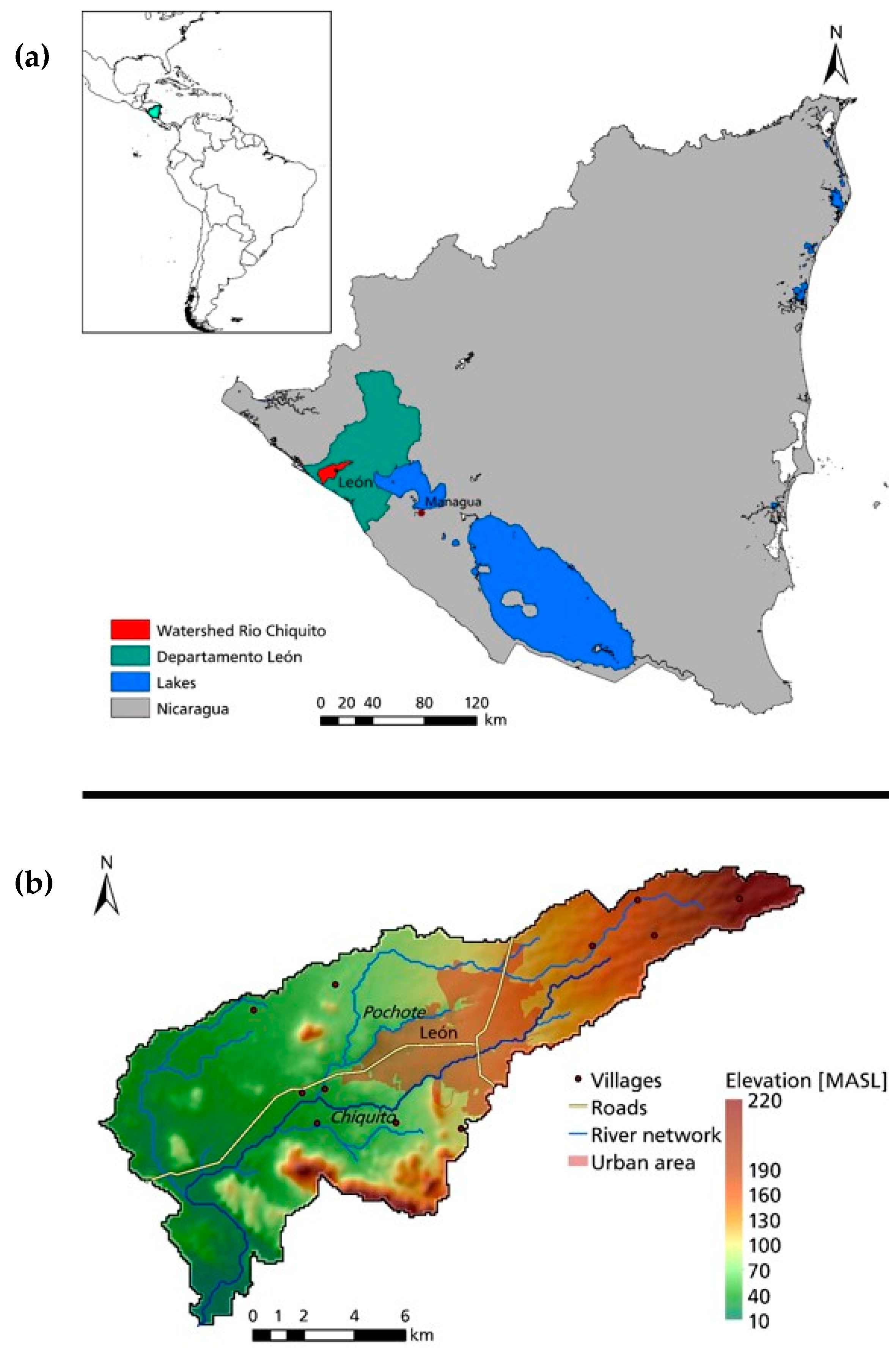
The Chiquito watershed is situated in the Northwest of Nicaragua in the Department León (see Figure 1a). The river drains over a length of 30 km in East-West direction from the Nicaraguan volcanic chain to the Pacific Ocean. Its source area is located about 2 km Northeast from the city of León, the capital of the equally named municipality. The total area of the watershed is 180.64 km2. The watershed is relatively flat, only in the north-eastern part the elevation increases up to 220 m a.s.l. (see Figure 1b). The Chiquito River traverses the city of León, where the majority of the population of the department lives. An important tributary to the Chiquito River, the Pochote River, originates at the northern city boundary of León and flows into the Chiquito River shortly after leaving the city. Out of town, the watershed is of rural character with a high use of agriculture. The watershed is located in the municipality León with a total population density of 2.33 inhabitants per hectare. Since 80 percent of the population lives in the city León, the urban density is 73.41 inhabitants per hectare, whereas the rural population density is 0.48 inhabitants per hectare [16].
The per capita annual water consumption of Nicaragua averages 252 m3. Thereby, households have a per capita consumption of 37 m3 per year, industry 6 m3 per year and agriculture consumes 209 m3 per capita and year [17]. The study area has a tropical savanna climate with a pronounced dry season from November to April and a rainy season from May to October, having an average monthly precipitation from 300 to 500 mm. The average temperature varies from 27 to 29° Celsius with the lowest values from December to February [16].
The watershed is characterized by agricultural use, whereby mainly a mosaic of cropland and vegetation dominates, being grassland, shrubland or forest, interrupted by herbaceous vegetation or forest. In the southwestern part, before the Chiquito River discharges into the Pacific Ocean, the river merges with a mangrove forest, known as the Natural Reserve Juan Venado Island, of high ecological value and importance for the tourism sector of Nicaragua [18]. The north-eastern area of the watershed contains an evergreen forest.
To analyse the watershed’s hydrological ecosystem services, the actual situation of the watershed is investigated. Especially, the main threats in the department León are degradation (loss of soil fertility) and erosion of soil. According to Galo Romero [19], the widespread agriculture and livestock farming cause soil degradation. In the course of this degradation, dust storms arise, which pose a health risk for the population. Therefore, research is focusing on alternative land management practices to maintain soils. Amongst others, these practices can be agroforestry or silvopasture combining forestry with pasture for livestock [19]. Water scarcity as well as floods are further risks. Although Nicaragua has large freshwater resources, water scarcity frequently becomes a problem. For instance, in the western part of Nicaragua, the population was threatened with water scarcity in 2015. Due to high temperatures caused by the phenomena of El Niño, water resources decreased strongly. The water scarcity is mainly related to global climate change resulting in reduced precipitation but also to the degradation of soils due to inappropriate agricultural use [20,21]. On the other hand, the department León is also vulnerable to floods, especially in the rainy season [22].
For model application, publically available and widely applied data was used that had been retrieved from the internet. Table 1 gives an overview of the required input data for all three models, its source and spatial resolution. Partly, the models require the same basic input data, which have to be pre-processed distinctly and saved in different formats.
The digital elevation model (DEM) used was retrieved from USGS HydroSHEDS and is a void-filled raster, whose no-data voids were filled using interpolation algorithms [23]. Before applying the DEM in the models, it was edited using the ESRI software ArcGIS. As can be seen from Table 1, the input raster files had originally different spatial resolutions. To receive homogenous modelling results, the input raster files are resampled to the DEM’s resolution. Therefore, all raster files have a pixel size of 90 m × 90 m.
The GlobCover map contains an error in the land use of the watershed. The city León, situated at the bank of the Chiquito River, is located in the land use raster west of its actual position. However, as other dominant landmarks (e.g., land-sea transitions, mountainous areas, mangroves) are situated geographically correct, the false location of the city of León is identified as a single georeferencing error that can be corrected. The position of León is corrected and the land use and land cover adapted by means of Google Earth. Moreover, the GlobCover map does not contain roads as land use. Sealed, major roads in the watershed are added to the raster dataset. The input data of the study area used for the SWAT model is shown in Table A1, the input data for the InVEST and RIOS models are shown in Table A2.
2.2. Software Used to Model Hydrological Ecosystem Services
Three different models are applied to the study area in Nicaragua, two special ecosystem service models and one traditional hydrological model. The widely used hydrological model, the Soil and Water Assessment Tool (SWAT) [29,30], was originally developed to predict the impacts of land management practices on water, sediment and agricultural chemical yields. However, several of the model outputs can be used to estimate and quantify the benefits of Hydrological Ecosystem Services. The models Integrated Valuation of Ecosystem Services and Tradeoffs (InVEST) [31,32] and the Resource Investment Optimization System (RIOS) [33] are developed especially for the modelling of ES by the Natural Capital Project (NatCap). In the following, the three models are briefly described and their specific characteristics highlighted.
The traditional hydrological model Soil and Water Assessment Tool—SWAT was developed by the USDA—Agricultural Research Service and the Texas A & M AgriLife Research [29,30]. For the present study, ArcSWAT version 2012.10.18 is used as a plugin for ESRI ArcGIS to set up the model and for the preparation of model input data. SWAT is a physically based, semi-distributed, continuous time model to simulate the impacts of land management practices on water, agricultural and chemical yields in large complex watersheds with varying soils, land cover and management conditions over long periods. The main components of SWAT are hydrology, weather, soil temperature and properties, plant growth, nutrients, pesticides, bacteria and pathogens as well as land management practices [34,35]. SWAT models the different physical processes in a watershed using various biophysical input data, such as weather, soil and land use information. To simulate the physical processes, SWAT divides the watershed into sub watersheds, which are further subdivided into hydrological response units (HRUs). These HRUs are lumped areas with homogenous land use, management conditions and soil characteristics [34,35]. The simulation of SWAT is divided into the land and water or routing phase of the hydrological cycle. Whereas the land phase controls the amount of water, sediment, nutrient and pesticide reaching the main channel in each sub watershed, the water or routing phase directs the movement of the water, sediment, etc. through the channel network of the watershed to the outlet [35]. The simulation of the land phase of the hydrological cycle is based on the water balance equation. Several of the SWAT model outputs can be used to estimate and quantify HES, such as water yield, sedimentation or water quality [36]. The translation of SWAT model outputs into HES requires post-processing, which is described in the following methodology section. SWAT has mostly been applied to evaluate provisioning and regulating services [6,7], such as freshwater production, water purification and sediment regulation. Specifically, SWAT can be used to determine a watershed’s capacity to provide HES. The main limitation of the SWAT model in HES modelling is that socio-economic data cannot be included and provision and benefits of HES cannot be linked. Therefore, a combination with a socio-economic analysis to compare the modelled service capacity with the societal demand and supply is reasonable [6].
The ecosystem service model Resource Investment Optimization System—RIOS [33] is an open-source, stand-alone software tool developed by NatCap. For this study, the RIOS version 1.1.16 is used. The RIOS model aims at the determination of locations for management activities to protect, maintain or restore ES, especially HES, in order to generate the greatest benefits for both people and nature focusing on low costs. RIOS is based on a conceptual approach operating independently of scale or location and, therefore, it can be used at continental, country, or regional scale. The tool works on annual or longer-term timescales and focuses on land management-based transitions. It uses widely available data on land use and management, climate, soil, topography and service demands. RIOS consists of two modules, which are, firstly, the Investment Portfolio Adviser and secondly, the Portfolio Translator. The Investment Portfolio Adviser determines a most efficient and effective set of investments in management activities with a specific budget, demonstrating where and in what activities investments are appropriate, which is the so-called Investment Portfolio. For this, the Investment Portfolio Adviser uses biophysical and social data, budget information and implementation costs for different activities. The first step in generating an Investment Portfolio is the definition of objectives the user wants to achieve. RIOS allows the user to select single or multiple objectives with or without weighting. The objectives provided by RIOS are erosion control for drinking water quality or reservoir maintenance, nutrient retention, flood mitigation, groundwater recharge enhancement, dry season base flow and biodiversity. For the achievement of these objectives, changes in the land management of the watershed may be required. Initial transitions in the vegetation or in land management practices can be caused by different activities. These transitions influence directly or indirectly hydrological processes and biodiversity. The transitions included in RIOS are: keep native vegetation, revegetation (assisted or unassisted), agricultural vegetation management, ditching, fertilizer and pasture management. Whereas these transitions are defined in the software, the selection of activities is determined by the user. This means that RIOS does not assist in the selection of activities but identifies where the selected activities obtain the greatest returns towards the user’s objectives [33].
Then, RIOS uses a ranking model to determine the areas, where investments have the highest return on investment. The approach is based on the condition that a limited set of biophysical and ecological factors determine the effectiveness of each transition in achieving each selected objective. Furthermore, a subset of landscape factors is defined having an impact on the effectiveness of activities and reflecting the landscape conditions and finally affecting each objective. The model approach assumes that the conditions of the surrounding landscape mainly determine the impacts of the transitions. Thereof, RIOS determines ranking scores for each user-defined spatial unit, the so-called pixel, derived from cell sizes of the input grid raster. Four components, being the conditions of the pixel itself and the conditions of the surrounding area are the determining factors for these scores [33].
The Portfolio Translator creates three major scenarios displayed as land cover maps based on the Investment Portfolio. The first scenario (baseline) contains the current land cover. The second scenario (transitioned) demonstrates new land cover combinations and protected areas caused by the implemented activities. The third scenario includes implemented activities but formerly protected areas are degraded demonstrating their benefits, when they are protected [33].
The ecosystem service model Integrated Valuation of Ecosystem Services and Tradeoffs—InVEST [32,37] is a set of different models to quantify and map ES. It is, as well as RIOS, an open-source, stand-alone software developed by NatCap. InVEST aims at the assessment of land cover changes on different ES in large watersheds comparing alternative land use scenarios. It aims to inform decision makers in natural resource management and to point out the impacts of changes in ecosystems to the benefits of people. The general approach of InVEST is based on production functions to quantify the impact of changes in the functions and structures of an ecosystem on the flows and outputs of ES. These functions are simplifications of common hydrological relationships [36]. InVEST calculates the results annually, based on land use information. The inputs are spatially explicit georeferenced rasterfiles or shapefiles and tables containing coefficients for each land cover type. The model calculates on a pixel basis, breaking up the watershed into pixels pursuant to the spatial resolution of the input data. These pixel results are aggregated to sub watershed results in further modelling steps. Since the spatial resolution is flexible, InVEST is capable to model at local, regional or global scale [36,38]. To visualize the outputs of intermediate modelling steps, final service levels and economic estimates, a mapping software or geographic information system (GIS) is necessary [38]. The set of InVEST models can be used to quantify and map terrestrial, freshwater and marine ecosystems. They can be categorized into three groups, which are supporting services, final services and tools to facilitate ES analyses [32]. Further information on the available set of InVEST models can be extracted from Sharp et al. [32] and Stanford University et al. [38]. For the presented study, two models of InVEST are selected: the Water Yield Model and the Sediment Delivery Ratio (SDR) Model.
The Water Yield Model estimates the annual average quantity of water provided by a watershed. This can be used, for instance, to evaluate potential hydropower production in a watershed. The results of the model illustrate which areas have the highest contribution to water yield and, thus, to hydropower production. Therefore, the Water Yield Model can assess different land use scenarios and their impacts on water yield. The model calculates the relative contribution of each land parcel to the annual average hydropower production, instead of directly modelling the effects of land use changes on hydropower [32,38]. This calculation, based on a gridded map, is divided into three steps. Firstly, the amount of water flowing off each pixel, which is the amount of precipitation less evapotranspiration, is calculated. Surface, lateral and base flow are not considered differentially. The pixel runoff is then summed up and averaged to sub watershed level. This is because the theory of the Water Yield Model is developed at sub watershed to watershed scale. Therefore, the results are only reliably interpretable on sub watershed to watershed scale. In the second step, the amount of surface water which is used for hydropower production is determined by subtracting water, consumed for other purposes, by the water scarcity model. The results of this step may be used to assess the possible water supply of the sub watershed and to determine whether water is scarce. Thirdly, the energy produced by the water reaching the reservoir and the energy’s value may be estimated. In general, the Water Yield Model is based on a simplification of the water cycle mainly including precipitation, transpiration and evaporation [32].
The input data required for the Water Yield Model consists of different raster datasets with values for each cell, shapefiles containing watershed and sub watershed polygons and tables in CSV-format. The tables contain biophysical coefficients for each land use class, a demand table comprising consumptive water use of each land use class and hydropower stations containing specific information. The output is divided into intermediate results per pixel and final outputs at sub watershed level. The final outputs are in shapefile format containing a table with the calculated values per sub watershed, such as the volume of water yield, the total water consumption and the total realized water supply volume for each sub watershed. If the hydropower valuation model is used, the table contains additionally the amount of energy produced and the economic value of the landscape per sub watershed to provide water for hydropower production over a specified time [32].
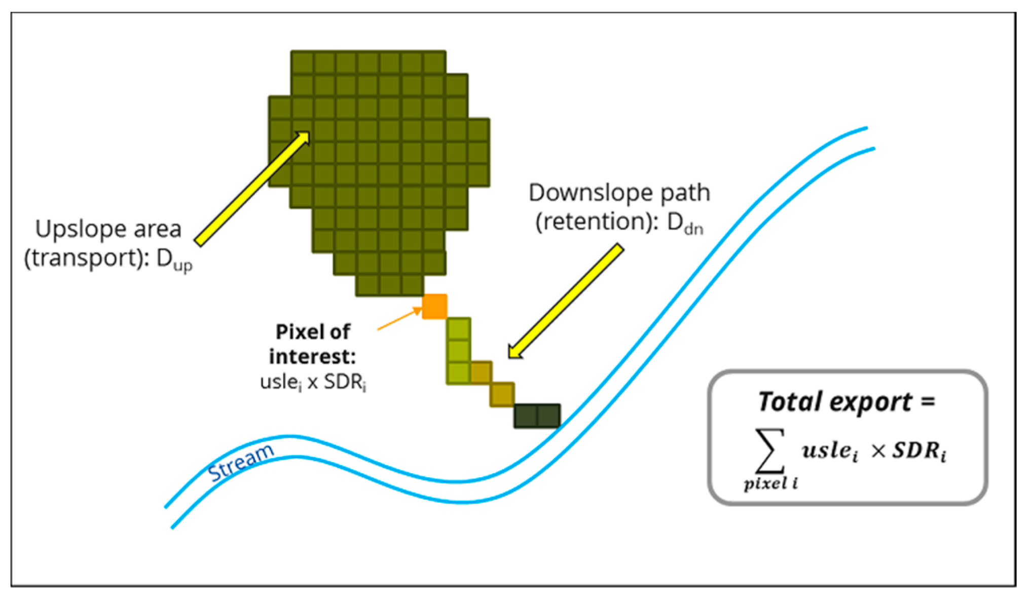
The Sediment Delivery Ratio Model (SDR Model) estimates the overland sediment generation and its delivery to the stream. The results of the model illustrate the ES of sediment retention in a watershed, which is significant for water quality and reservoir management. Changes in land use or alterations in land management practices can influence sediment export in a watershed. The SDR Model focuses on overland erosion processes. The biophysical model is spatially explicit and adopts the spatial resolution of the input DEM raster. Firstly, the model calculates the annual loss of each pixel with the Revised Universal Soil Loss Equation (RUSLE; [39]). The model determines the sediment delivery ratio (SDR) in two steps basing on a function of upslope area and downslope flow path, which is illustrated in Figure 2. In the first step, a connectivity index is calculated, from which, in a second step, the sediment delivery ratio is derived for each pixel. With the sediment delivery ratio and the amount of annual soil loss calculated with the RUSLE equation, the sediment load is determined. The SDR Model requires, such as the water yield model, different biophysical input datasets in georeferenced raster, shapefile and table format.
The required raster datasets are a DEM, the rainfall erosivity index, the soil erodibility and the land use and land cover. Optionally, a drainage layer can be used to include artificial connectivity to a stream, such as urban areas or roads. The outputs of the SDR Model are divided into intermediate and final results. The intermediate results are raster sets containing results per pixel, which should not be used for an evaluative interpretation because the model assumptions are based on processes at sub watershed level and results per watershed or sub watershed in a shapefile. This shapefile contains the total amount of sediment exported to the stream, the total amount of potential soil loss and the sediment retention in tons per watershed. The outputs of the SDR model, being the annual sediment load delivered to the stream and the amount of sediment eroded in the watershed and kept by vegetation and topography, can be used to evaluate the ES of sediment retention. For a quantitative valuation, the model computes the sediment retention as the difference to a hypothetical watershed of bare soil. Moreover, an index of sediment retention is calculated, identifying areas that contribute more to retention with reference to bare soil. This index can be used for a qualitative assessment. See Sharp et al. [32] for a detailed description of the SDR Model.
2.3. Methodology-Application of the Models, Data Pre- and Post-Processing
The three models are compared theoretically and practically (in application to a case study) in the following to evaluate their suitability for decision-making. The theoretical comparison is based on different qualitative and quantitative criteria to highlight the differences or similarities between the models. These criteria are the model type, the original model purpose and the general model concept as well as the model approach reflecting the structure of the model. Furthermore, the underlying equations, the temporal and spatial resolution and the scale of the results are considered. Besides, it is examined, which ES are assessed and whether it is possible to include beneficiaries. Another point of the theoretical comparison considers the mapping and the displaying of multiple ES. Moreover, the model limitations and the required input data are compared. The theoretical comparison is complemented with the practical application of the three models for a study area in Nicaragua. Then, the results of the practical application are compared concerning different criteria. This comparison focuses on the application and the results of the models as well as on the model application effort. The qualitative and quantitative criteria of the practical comparison are the application objective, which can be achieved with the model, the types of results, the kind of visualization, how and whether beneficiaries are included and areas of provision and use of ES can be distinguished. Another criterion is the possibility to combine the models with each other. Since uncertainty is an important point in modelling, this issue is also considered in the comparison to show to what extent and how the models deal with this issue. Moreover, the effort to apply the three models to the study area is compared. The evaluation criteria here are data requirement and necessary pre-processing, data availability, training effort to apply the model and the presence of instructions or user manuals. Finally, the time required to apply the three models is compared.
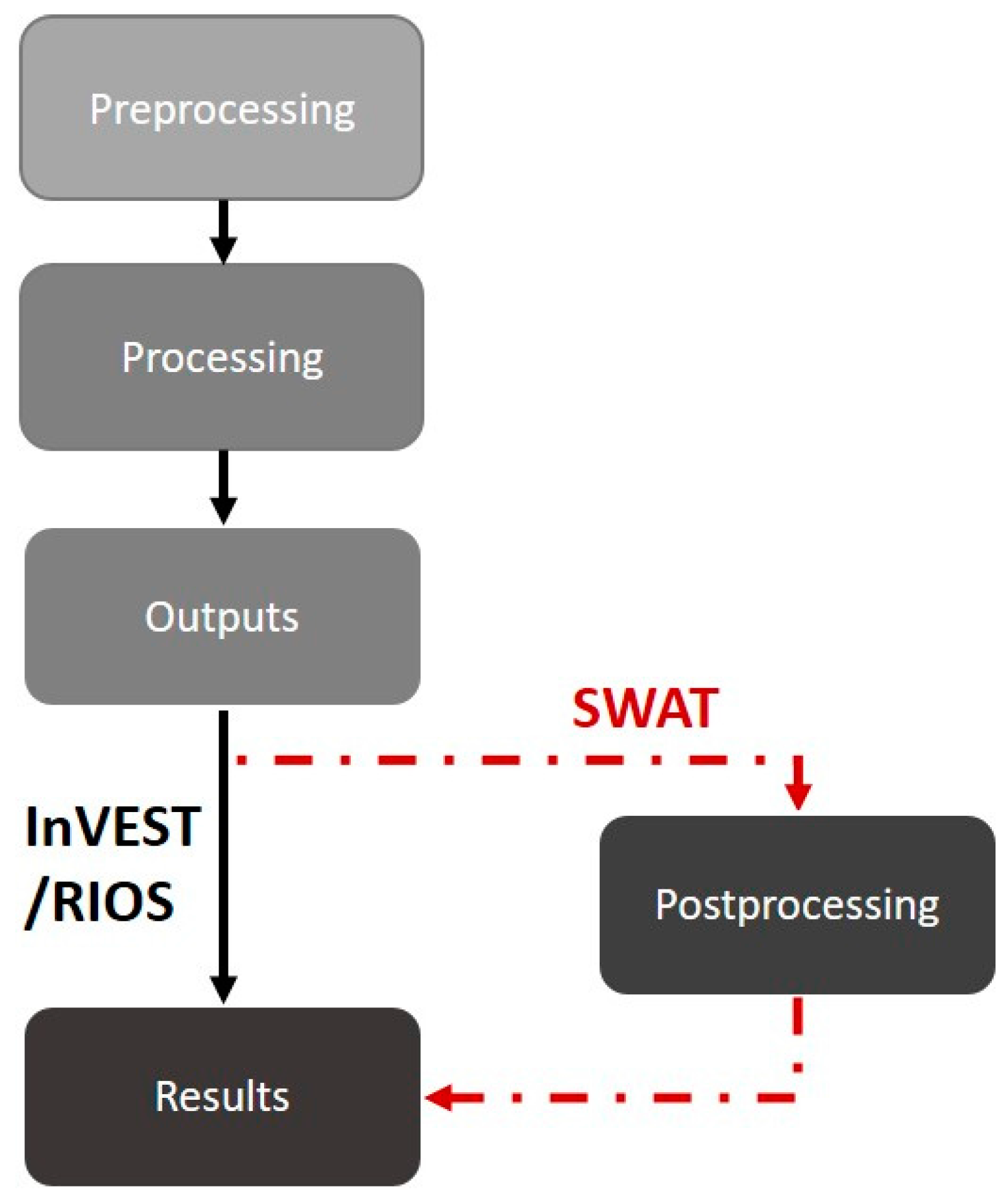
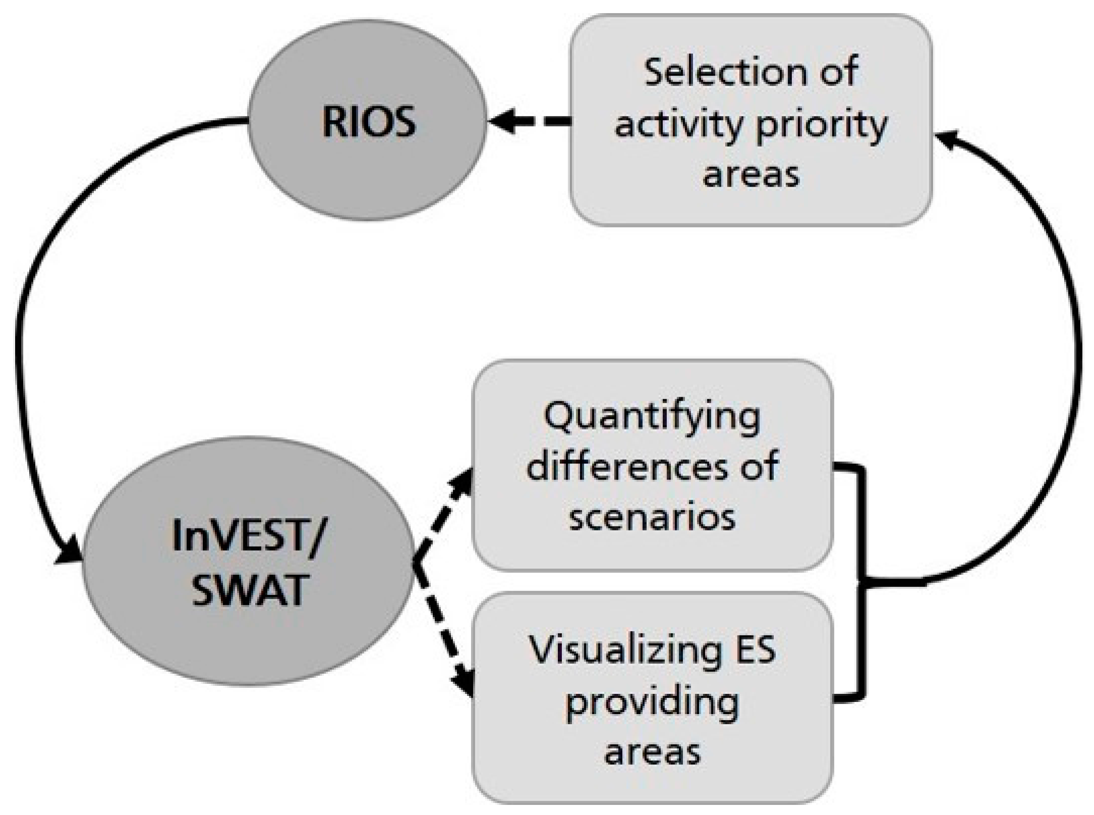
In addition to the theoretical comparison and their underlying structures, the models are applied to a study area in Nicaragua. Since the three compared models vary in their theoretical concepts and structures as well as in their application, different approaches are necessary for the practical comparison. As can be seen from Figure 3, the general approach for the models InVEST and RIOS is the same. The output of InVEST is in shapefile format and can be displayed by means of a GIS representing the capacity, demand and supply of a specific ES. RIOS generates an Investment Portfolio, containing raster files and tables with the results. These are the locations for activities to restore or protect the selected ES, the budget spent and alternative land use scenarios, amongst other information. The results can be visualized with a GIS. Therefore, InVEST and RIOS require no post-processing of their outputs. In contrast, the application of SWAT requires post-processing to translate the model outputs in ES, since the original purpose of SWAT is predicting the impacts of land management practices on water, sediment and agricultural chemical yield in large watersheds. The visualization of the results requires for all three models the use of a GIS.
Several of the SWAT model outputs can be used to estimate and quantify the capacity of ES. For the study area in Nicaragua, the HES of water flow regulation and sediment retention are analysed with the three models. Therefore, appropriate indicators from the SWAT model output have to be selected. These variables can be used to indicate HES either in combination or alone. There are different approaches to translate SWAT outputs into HES. The approach for the study area in Nicaragua follows Schmalz et al. [7]. Table 2 shows the variables selected to represent the ES of water flow regulation and sediment retention. As can be seen from Table 2, the water flow regulation is composed by variables reflecting the water cycle, which are the surface and lateral flow, the soil water content and the groundwater contribution indicating the quantity of water retention and the retention capacity of the surface and underlying soils. To represent the HES of sediment retention, the sediment yield transported to the main channel is selected. It can be used to indicate areas with little sediment export and, thus, a high sediment retention. For the mapping of ES, the hydrological response unit is suitable due to the finer spatial resolution compared to the sub watershed, which enables a more detailed display of the results.
The output of each variable is averaged over the last five years of the simulation period, which is from 2008 to 2013, to compensate annual variabilities. The outputs of each variable are assigned to a ranking scale from one (very low potential to provide ES) to five (very high potential) to make different HES comparable, proposed by Burkhard et al. [41]. Each variable is subdivided into value ranges assigned to the ranking scale, using the statistical data mean, maximum and minimum to create class breaks. To receive the potential of water flow regulation, all ranking values of all variables are averaged. The result is a ranking value for each HRU reflecting its capacity to provide water flow regulation. Since the sediment retention is determined with one SWAT output variable, it is not necessary to average the ranking values. The ranking values are visualized on HRU basis using a GIS.
3. Results
The theoretical comparison focuses on the theoretical model fundamentals and consists of the comparison points described in the methodology section. The following section focuses on the results of the practical application to the study area in Nicaragua.
As described in the methodology section, different variables of the SWAT output are selected and post-processed to display HES. Figure 4 shows the results generated with SWAT, demonstrating the capacity of the watershed to provide the HES of sediment retention and water flow regulation. These functions are only HES, when people are present who potentially could benefit from them. Since it is not possible to integrate social data in the SWAT model, a visual comparison is performed, illustrated in Figure 4 (right side). Therefore, the capacity maps are compared with the beneficiaries’ rasters created for the RIOS model. Since 80 percent of the population in the watershed lives in the city of León, this area is strongly weighted. Therefore, a second raster is created containing only the rural population. For the visual comparison of the SWAT results, a raster is created containing the population per HRU. As can be seen from Figure 4a, large areas of the watershed provide a very high capacity to retain sediment. However, sediment retention especially takes place in the northern part of the watershed with a low number of beneficiaries. In the eastern part of the watershed, an area with high retention and a medium number of beneficiaries is located. This is also a benefiting area (see beneficiaries rural) of water flow regulation (Figure 4b) with a medium to high capacity. Furthermore, the people in the east of León (see beneficiaries all) benefit from a high water flow regulation. In contrast, areas with a very high water flow regulation located in the south-west of León, have a low to medium number of beneficiaries (see beneficiaries rural).
Since RIOS consists of two modules, the Investment Portfolio Adviser and the Portfolio Translator, there are two different outputs. RIOS determines areas for the implementation of activities to restore or maintain different ES or objectives. For the study area in Nicaragua, the objectives erosion control for drinking water quality, flood mitigation and dry season base flow are selected. RIOS determines areas, where activities to achieve these objectives are best situated, with regard to the benefits of people, nature and costs. Therefore, one result of RIOS is a budget report showing the costs and the converted area for each activity. Because there are two different raster images representing all and rural beneficiaries, two simulations of RIOS are run. Since the results are very similar, only the results for all beneficiaries are presented here. Figure 5 shows the implemented activities. Mainly, grass strips, protection and in some areas, agroforestry is implemented. Grass strips are only allowed on areas with a slope smaller than twelve percent. Therefore, in the steeper areas agroforestry is prioritized. Protection is focused in two areas with native vegetation, which are tropical evergreen forest in the NE and swamp forest in the SW of the watershed. Reforestation is implemented at shrub areas. Riparian management is mainly chosen for the western part of the watershed in downstream areas.
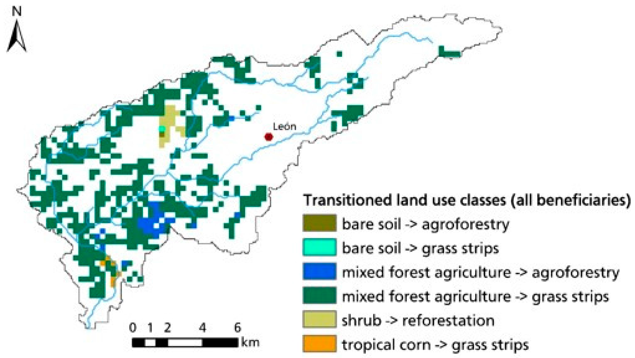
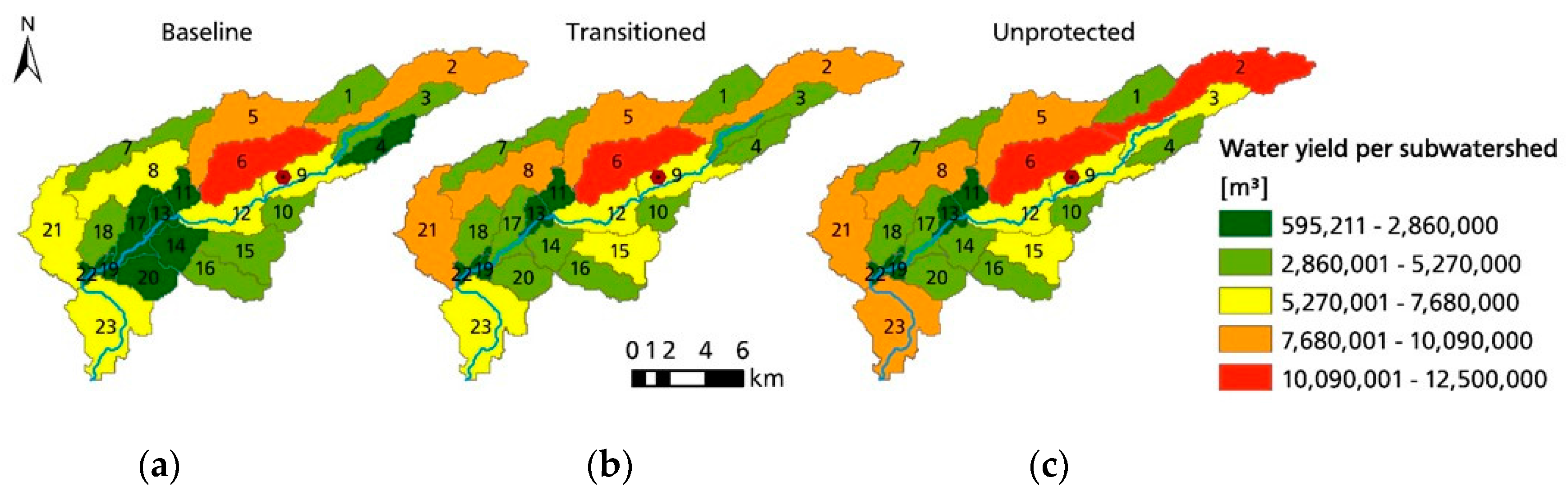
The second output of RIOS, generated by the Portfolio Translator, contains three land cover scenarios. These are the baseline scenario with the starting land cover, the transitioned scenario showing the transitions in land cover caused by the activities and an unprotected scenario indicating which changes in land cover are expectable, when protected land use classes are degraded. Figure 6 visualizes the land use classes, which are changed by the implemented activities.
The impacts of the implemented activities by RIOS on the HES can be evaluated with other models, for example with the InVEST Water Yield Model using the generated land use scenarios as inputs. This is shown in Figure 7, which contains the results of InVEST for the three land use scenarios generated by RIOS. As can be seen from Figure 7, the implemented activities have an impact on the water yield of the sub watersheds. The sub watersheds 4, 8, 14, 15, 17, 18, 20 and 21 of the transitioned scenario have a greater water yield than the baseline scenario. Considering the objective of base flow enhancement and drinking water supply, this is beneficial. In contrast, an increase in water yield may also be adverse considering flood mitigation. Thus, in order to interpret the modelling results in this context, a finer temporal solution of input and output data is required that provides information on how water yield is seasonally distributed. With the current version of InVEST, this is not possible.
The third scenario includes the transitioned areas but formerly protected areas are degraded. This degradation influences the water yield of the sub watersheds located in these areas. These are the sub watersheds 2, 3 and 23 having an increase in water yield due to their reduced water retention capacity. However, the results are annually and do not reflect seasonal variability, for example due to rainy and dry seasons.
Furthermore, the InVEST Water Yield Model is run with the original input data, additionally using a water demand table to analyse water scarcity. Figure 8 shows the results of this run, illustrating the available water yield per sub watershed, the water consumption per sub watershed and the water supply per sub watershed which is the available water yield minus the water consumption. According to Figure 8, the sub watersheds with the highest provided water yield are 6, 2, 5 and 8. The water consumption is highest in the urban area of León (sub watersheds 6, 9, 10 and 12). However, a comparison of the maximum values of water demand and the values of water yield shows that the maximum of water demand (1,851,418 m3 per sub watershed) lies in the lowest interval of the water supply. Therefore, it can be assumed that the water yield exceeds the demand, as visualized in the image at the bottom of Figure 8. A relevant decrease in the water amount can only be determined in the sub watersheds 4 and 12. However, it should be taken into account that the results are annual averages, again not representing seasonal variability. SWAT has the potential to provide information of seasonal variability (and even on daily time steps) of model results but for the comparison of model applicability presented here, this has not been considered.
Furthermore, the InVEST Sediment Delivery Ratio model or SDR model is applied for the study area in Nicaragua. The SDR model estimates sediment export and retention for each sub watershed, as illustrated in Figure 9. The sediment export in tons per sub watershed (left side of Figure 9) is highest in the sub watersheds 8, 16, 20 and high in the numbers 6, 14, 15, 21 and 23, what is similar to the result of SWAT (see Figure 4). The sediment retention (right side of Figure 9), expressed in tons per sub watershed, is estimated in reference to a degraded watershed with bare soil. The value of sediment retention is based upon the difference between sediment export from the bare soil watershed and the input scenario. This may be the reason, why sediment retention is highest in the sub watersheds 16 and 14, 15, 20 and 23, although these are the sub watersheds with the highest sediment export to the stream. Due to the calculation of sediment retention in reference to a bare soil watershed, these sub watersheds are considered as retention areas, because the soil loss by the current land use is far less than the soil loss of a bare soil watershed.
As can be seen from the results, the three models can be used to achieve different objectives. SWAT allows analysing the capacity of HES in detail. In contrast, InVEST gives a quick overview of different ES. RIOS can be used to determine activity areas for the protection and restoration, especially, for HES.
4. Discussion
The comparison of the three models shows that differences between their methodological approaches and results exist. The differences of the models, their results and the specific application effort, in reference to the practical application are summarized in Table 3 and discussed in the following.
Due to the different input data and model concepts, a direct comparison of the model results is difficult. A direct comparison to verify the results is only recommendable, when the same input data set for all models is used. However, the comparison of the sediment export of the InVEST SDR Model and the sediment retention capacity calculated by SWAT shows that SWAT and InVEST deliver similar results for the southern and western parts of the watershed. These differences in results may be due to the different time of acquisition of the input data. Nevertheless, both results can be used to determine areas with a high sediment retention or sediment export potential. In contrast to SWAT, the InVEST SDR model additionally simulates a sediment retention scenario. These scenarios can be used, in comparison with the modelled sediment export, to determine areas of priority that should be protected or to improve the land use conditions relating to sediment retention.
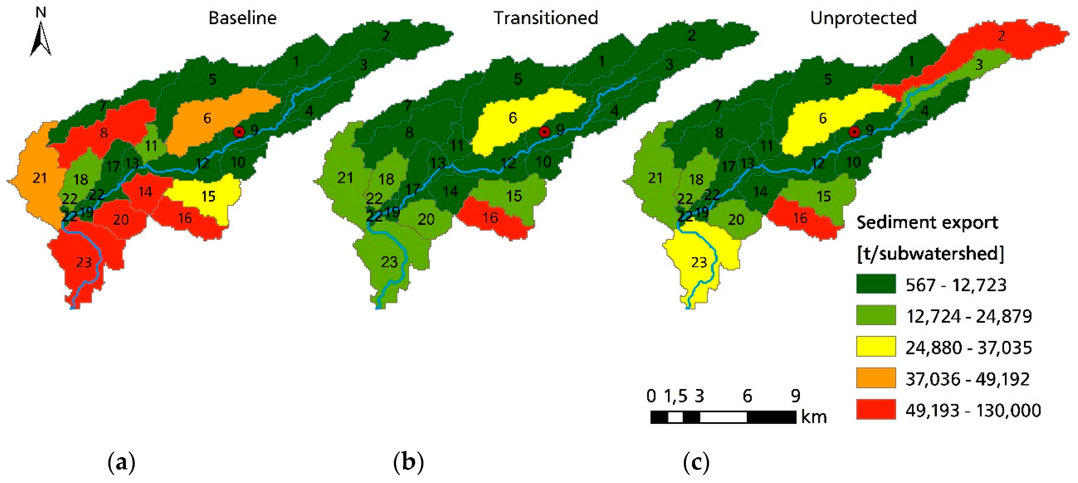
The southern part of the watershed (sub watersheds 23, 20, 14, 15, 16) has, according to the results of InVEST and SWAT a high sediment export or a low capacity of sediment retention but the current conditions provide a higher retention capacity than a degraded, bare soil would do. Therefore, it can be assumed that a transition in land use, for example to agroforestry, would lead to a better sediment retention capacity in this area. In this part of the watershed, agroforestry and grass strips are suggested by the RIOS model to improve sediment and water flow retention (see Figure 5). The results of RIOS (suggested land use transitions) are then evaluated by the InVEST SDR model. As can be seen from Figure 10, the activities of agroforestry and grass strips improve the sediment retention in the southern part of the watershed. Hence, InVEST and SWAT give consistent predictions for the capacity of sediment retention and the activities implemented by RIOS potentially improve sediment retention.
For decision support, the InVEST SDR model can be especially useful to give a relatively quick overview of the current sediment retention capacity and areas with potential for improvement in service provision. By means of this, activities for RIOS can be developed. These activities for land use transitions or protection can then be implemented in priority areas suggested by RIOS. Subsequently, the effects of the implemented activities can be evaluated with InVEST to quantify potential changes in ecosystem services. In the case of sediment retention, the implemented activities improve sediment retention capacity. Thus, the results of InVEST and RIOS could be used to determine ecosystem service supply areas for Payments for Hydrological Ecosystem Services (PHES). However, for the implementation of PHES a finer resolution of the results than the sub watershed level is necessary. This can be achieved using the SWAT model to assess different land use scenarios with implemented activities and their impacts on sediment loadings, because SWAT produces results at the level of hydrological response units that are of finer resolution than the sub watershed level.
The results for water yield of InVEST and the capacity of water flow regulation of SWAT differ. Firstly, because the results are calculated with different conceptual approaches. Whereas the water flow regulation calculated by SWAT is based on variables of soil water content, surface and lateral flow as well as groundwater contribution, the water yield of InVEST is merely calculated as precipitation less evapotranspiration, thus a simplified water balance. Furthermore, different input data, due to availability, is used for the simulation. Therefore, a direct comparison of the results is not recommendable. Thus, a comparison of Figure 4 and Figure 8 illustrates the differences in model results. However, sub watersheds 5, 6 and 8 show—in both outputs—similar results, a low to medium capacity of water flow regulation and corresponding a high water yield.
SWAT is not able to include socio-economic data or beneficiaries of ecosystem services, whereas InVEST calculates both water yield and water supply, which allows conclusions on water scarcity. Thus, SWAT only allows conclusions on the watershed’s capacity to provide water flow regulation. Merely a visual comparison with the locations of beneficiaries can be performed. For decision-making, the results of InVEST provide a good overview of the water provision in the watershed. The evaluation of the RIOS results with InVEST reveals that the implemented activities partially lead to an increase in water yield (see Figure 8). This may be due to the selection of the objective base flow enhancement. However, the same activities lead to a reduction of sediment export. This would normally suggest that surface flow and thus water yield are reduced. Therefore, the implemented activities should be verified for reliable results.
In summary, the results of SWAT and InVEST for water flow regulation and water yield should be used for different questions. InVEST can be used for an overview of water yield and water supply. SWAT can be used if different scenarios reflecting the heterogeneity of land use patterns should be evaluated (see Figure 11). This is useful when farmers, settlements and their agricultural land use in service provision areas should be identified to implement PHES.
While SWAT and InVEST are based on similar conceptual approaches to model hydrological processes, RIOS follows a different approach, determining scores for particular activities using biophysical input data. However, the SWAT model is more complex and thus it models hydrological processes in more physically-based detail. This requires a large number of input data in comparison to the other models. Since the RIOS model is based on a ranking approach combining biophysical and social input data, it does not model underlying hydrological processes and HES. It uses input data to determine activity preference areas for HES.
The application effort for the SWAT model is particularly higher. This is due to the high time requirement for the pre-processing of input data, the training effort to apply the model and the necessary post-processing to quantify and visualize HES. Since different variables of the SWAT output are selected as indicators of a specific HES, the variables are transformed to a ranking scale (five classes), reflecting relative service capacity. The chosen class limits have a strong influence on the result. The display of spatial variabilities can be affected by the chosen class limits. Other approaches to model HES with SWAT modify and complement the model. This requires specific knowledge and thus, complicates the application for decision makers. The InVEST and RIOS models are more user-friendly due to their fewer input data requirements and the lower training effort to apply them.
The main difficulty in all model’s application is data availability. Especially, for the SWAT model, the required data is not widely (publicly and free of charge) available. The reason for this is on the one hand, the complexity of the model requiring a large number of different variables, on the other hand, the location of the study area in Nicaragua. The data situation in developing countries is mostly poorer than in industrialized countries. The data situation is particularly high in the United States, especially for the SWAT model, which is developed and commonly applied there. Furthermore, available data is often not readily usable in the models and needs pre-processing. Additionally, open-source data, which is globally available, has a coarse resolution. This is particularly adverse for the modelling on a regional or local scale (<100 km2), because land use and land cover data are displayed in a coarse resolution, not reflecting the heterogeneity of land use patterns appropriately. Recommendations for local land use improvements remains therefore challenging. Since InVEST and RIOS are developed for decision makers and with focus on an application in developing countries, they use more commonly available data. However, the application of the RIOS model needs a table, containing user-specified activities, to cause the desired transitions. Hence, previous knowledge of the watershed or the target area is required to determine appropriate activities. It is advantageous, thus, to know, which problems or HES occur in the area to define activities and specify the land use classes suitable for the respective activity. For this, local knowledge or the application of a model, which maps HES, is helpful.
Considering these points, recommendations for the application of the models can be derived. The SWAT model, a traditional hydrological model, is generally suitable to quantify and map the capacity of HES. Since it is not able to include data regarding potential beneficiaries of HES and its focus on hydrological processes, post-processing for the display of HES is required. This complicates its immediate application for decision makers. However, a main advantage of the model is that it is based on widely accepted and applied hydrological process knowledge and thus, simulates these processes more detailed and, at least partly, physically-based. The model complexity and the large amount of required input data are detrimental to the application in decision-making processes. Therefore, SWAT is recommended for a detailed analysis of specific HES, if sufficient data, time and hydrological expertise are available.
In contrast to SWAT, RIOS and InVEST can be applied in situations with a limited availability of data and time. Since the approach of InVEST is simpler than the concept of SWAT, it can be used to give a quick overview of different HES. Furthermore, it allows partially an economic evaluation and is capable to model service demand and supply. The disadvantage of InVEST is that the results, up to now, are only reliable on sub watershed basis, not reflecting finer spatial patterns. Besides, it calculates on an annual basis, thus seasonal variability is not considered. This is a clear disadvantage when ES also follow a seasonal variability.
The RIOS model is especially useful to locate activity preference areas for the maintenance and restoration of multiple HES. The medium data and time requirement facilitates its application for decision makers. A difficulty is the determination of appropriate activities and their implementation on different land use classes. Furthermore, the impacts of the implemented activities cannot be evaluated with the RIOS model itself. Therefore, it may be useful to combine RIOS with other models, for example with InVEST or SWAT. It is also possible to use SWAT to show the impacts of different land use scenarios provided by RIOS. The results of InVEST and SWAT can help to define the activities and choose the objectives in RIOS. Figure 11 illustrates a possible combination of the models. RIOS can be used with InVEST or SWAT in an iterative process, for example, to determine activity preference areas for a water fund and to evaluate the scenarios of alternative land use and management scenarios. For this, InVEST is especially suitable because it requires almost the same input data as RIOS. Moreover, the outputs of RIOS can serve as direct input for InVEST. Furthermore, the results of InVEST or SWAT can assist in the selection of activities in RIOS. Therefore, a combination of the models may help decision makers to get a good overview of the HES provided in a watershed and where activities to restore or protect them can be implemented.
The InVEST and RIOS models represent already a good approach for the inclusion of beneficiaries. Other approaches, like the probabilistic ARIES model [42] simulate and visualize areas of service provision, benefits and flow paths between the use and source regions. However, ARIES can only apply biophysical relationships if sufficient data is available. Unless it relies on probabilistic relationships from data of other sites to link spatial input data and ES values.
5. Conclusions
The comparison of the underlying theory of the three models shows that the models differ in their methodological approaches, practical application efforts and consequently in their results. Due to this, it is recommendable to apply the models for different purposes and decision-making contexts. Since SWAT bases on widely accepted algorithms to model hydrological processes, it is suitable to evaluate different scenarios of land use on a fine spatial resolution and allows also a higher temporal resolution of outputs. This is recommendable when enough time, due to the high application effort, and input data are available. RIOS follows a ranking approach selecting areas to implement activities for improvement of ecosystem services, which is useful for the implementation of PHES. In contrast to SWAT, the InVEST model can be applied to model different ecosystem services directly. Basing on simplified hydrological process representation, InVEST can be used to quantify and map different ecosystem services relatively fast. Furthermore, InVEST or SWAT can be used to evaluate the results simulated with RIOS. Especially the combination of InVEST and RIOS is recommendable, since they require mainly the same input data.
In summary, provisioning and regulating HES can already be modelled in a useful way. However, the model application in decision-making processes remains challenging, mainly due to a high application effort. Since the quantification and mapping of HES represent a good opportunity for the protection of ES and the maintenance of natural resources for human well-being, future research in HES modelling should dedicate to the development of reliable, easy applicable tools, which base on hydrological process knowledge, incorporate the beneficiaries of services and require few and widely available input data. For future HES research, the data situation and availability should be improved. The implementation of monitoring programs could help to improve the data situation and to improve the knowledge on processes that influence water flow and quality, except of land use and land cover. Therefore, additional research ought to be dedicated to other influence factors on HES than land use and land cover.
Acknowledgments
We acknowledge support from the German Research Foundation and the Open Access Publishing Fund of Technische Universität Darmstadt. Further we want to express our gratitude to three anonymous reviewers for their valuable comments on the manuscript.
Author Contributions
All authors contributed equally.
Conflicts of Interest
The authors declare no conflict of interest.
Appendix A

Table A1.
SWAT soil input variables.
| Variable | Definition | Obtained from or Calculated by |
|---|---|---|
| HYDGRP | Soil hydrological group (A, B, C, D), based on infiltration characteristics | Determination suggested by Arnold et al. [40] but required data not available; therefore simplified determination proposed by Environment and Natural Resources Trust Fund (n.d.) using soil texture provided by HWSD |
| SOL_ZMX | Maximum rooting depth of the soil profile (mm) | Reference soil depth (REF_DEPTH from HWSD, 1000 mm), because no other data available |
| SOL_Z1,2 | Depth from soil surface to bottom of layer (mm) | Topsoil (300 mm) and subsoil depth (700 mm) of HWSD |
| SOL_BD1,2 | Moist bulk density (Mg/m3 or g/cm3) | Reference bulk density from HWSD calculated with equation from Saxton and Rawls [43] (T/S_REF_BULK_DENSITY) |
| SOL_AWC1,2 | Available water capacity of the soil layer (mm H2O/mm soil) | Calculated by SPAW—Soil Water Characteristics [44] |
| SOL_K1,2 | Saturated hydraulic conductivity (mm/h) | Calculated by SPAW—Soil Water Characteristics [44] |
| SOL_CBN1,2 | Organic carbon content (% soil weight) | T_OC and S_OC from HWSD |
| SOL_CLAY1,2 | Clay content (% soil weight) | T_CLAY and S_CLAY from HWSD |
| SOL_SILT1,2 | Silt content (% soil weight) | T_SILT and S_SILT from HWSD |
| SOL_SAND1,2 | Sand content (% soil weight) | T_SAND and S_SAND from HWSD |
| SOL_ROCK1,2 | Rock fragment content (% total weight) | T_GRAVEL and S_GRAVEL from HWSD |
| SOL_ALB1 | Moist soil albedo | Calculated by the equation from Post et al. (2000): with data from [45] |
| USLE_K1 | USLE equation soil erodibility K factor | Calculated with the equations of Williams [46] given in [40] using the sand, silt, clay and organic carbon content |
Table A2.
RIOS and InVEST input raster data.
| Data | Definition | Obtained from or Calculated by |
|---|---|---|
| Average annual rainfall | Mean annual rainfall depth in mm for each cell | WorldClim (Bioclimatic variables for tile 23), annual average from 1960–1990 [27] |
| Rainfall depth or precipitation of wettest month | Rainfall depth influences the amount of runoff of each cell. If the rainfall depth is not available, the mean precipitation of the wettest month can be used (mm) [33] | WorldClim (Bioclimatic variables for tile 23), annual average from 1960–1990 [27] |
| Mean annual actual evapotranspiration (AET) | Mean annual values for each cell in mm | CGIAR-CSI, annual average from 1950–2000 [28] |
| Reference evapotranspiration (only InVEST) | Average annual reference evapotranspiration—in mm—being the potential loss of water from soil evaporation and alfalfa/grass transpiration if sufficient water is available; the equations (Penman-Monteith, Hargreaves etc.) for potential evapotranspiration (PET) are suggested, therefore the PET raster of CGIAR-CSI can be used | CGIAR-CSI, annual average potential evapotranspiration from 1950–2000 [47] |
| Rainfall erosivity | Rainfall erosivity index R depending on the intensity and duration of rainfall in | Calculated using WorldClim data with an equation proposed by Mikhailova et al. [48] |
| Soil erodibility | Soil erodibility K measures the susceptibility of soil particles to erosion in [33] | Calculated using HWSD according to Sharp et al. [32] |
| Soil depth | Average soil depth for each cell in mm | Obtained from HWSD data |
| Soil texture (only RIOS) | Index value for each cell representing the soil texture class | Derived from HWSD |
| Plant available water fraction (only InVEST) | PAWC is the fraction of water stored in the profile and available for plants’ use [33] | Calculated with SWAT input variable SOL_AWC (from SPAW) by adding up the SOL_AWC values across horizons |
| Location and number of beneficiaries (only RIOS) | Location and number of beneficiaries depend on the chosen objective; different raster files for different objectives: erosion control: population density (rural and all beneficiaries); base flow and flood mitigation: population downstream (rural and all) | Calculated with population density [16] |
References
- Crutzen, P.J. Geology of mankind. Nature 2002, 415, 23. [Google Scholar] [CrossRef] [PubMed]
- Millennium Ecosystem Assessment. Ecosystems and Human Well-Being: Synthesis; Island Press: Washington, DC, USA, 2005. [Google Scholar]
- Hack, J. Application of payments for hydrological ecosystem services to solve problems of fit and interplay in integrated water resources management. Water Int. 2015, 40, 929–948. [Google Scholar] [CrossRef]
- Brauman, K.A.; Daily, G.C.; Duarte, T.K.K.; Mooney, H.A. The Nature and Value of Ecosystem Services: An Overview Highlighting Hydrologic Services. Annu. Rev. Environ. Resour. 2007, 32, 67–98. [Google Scholar] [CrossRef]
- Duku, C.; Rathjens, H.; Zwart, S.J.; Hein, L. Towards ecosystem accounting: A comprehensive approach to modelling multiple hydrological ecosystem services. Hydrol. Earth Syst. Sci. 2015, 19, 4377–4396. [Google Scholar] [CrossRef]
- Francesconi, W.; Srinivasan, R.; Pérez-Minana, E.; Willcock, S.P.; Quintero, M.; Pérez-Miñana, E.; Willcock, S.P.; Quintero, M. Using the Soil and Water Assessment Tool (SWAT) to model ecosystem services: A systematic review. J. Hydrol. 2016, 535, 625–636. [Google Scholar] [CrossRef]
- Schmalz, B.; Kruse, M.; Kiesel, J.; Müller, F.; Fohrer, N. Water-related ecosystem services in Western Siberian lowland basins - Analysing and mapping spatial and seasonal effects on regulating services based on ecohydrological modelling results. Ecol. Indic. 2016, 71, 55–65. [Google Scholar] [CrossRef]
- Swallow, B.M.; Sang, J.K.; Nyabenge, M.; Bundotich, D.K.; Duraiappah, A.K.; Yatich, T.B. Tradeoffs, synergies and traps among ecosystem services in the Lake Victoria basin of East Africa. Environ. Sci. Policy 2009, 12, 504–519. [Google Scholar] [CrossRef]
- Hamel, P.; Chaplin-Kramer, R.; Sim, S.; Mueller, C. A new approach to modeling the sediment retention service (InVEST 3.0): Case study of the Cape Fear catchment, North Carolina, USA. Sci. Total Environ. 2015, 524, 166–177. [Google Scholar] [CrossRef] [PubMed]
- Nelson, E.; Mendoza, G.; Regetz, J.; Polasky, S.; Tallis, H.; Cameron, R.; Chan, K.M.A.; Daily, G.C.; Goldstein, J.; Kareiva, P.M.; Lonsdorf, E.; et al. Modeling multiple ecosystem services, biodiversity conservation, commodity production, and tradeoffs at landscape scales. Front. Ecol. Environ. 2009, 7, 4–11. [Google Scholar] [CrossRef]
- Nourani, V.; Roughani, A.; Gebremichael, M. Topmodel capability for rainfall-runoff modeling of the Ammameh watershed at different time scales using different terrain algorithms. J. Urban Environ. Eng. 2011, 5, 1–14. [Google Scholar] [CrossRef]
- Terrado, M.; Acuña, V.; Ennaanay, D.; Tallis, H.; Sabater, S. Impact of climate extremes on hydrological ecosystem services in a heavily humanized Mediterranean basin. Ecol. Indic. 2014, 37, 199–209. [Google Scholar] [CrossRef]
- Bagstad, K.J.; Semmens, D.J.; Waage, S.; Winthrop, R. A comparative assessment of decision-support tools for ecosystem services quantification and valuation. Ecosyst. Serv. 2013, 5, 27–39. [Google Scholar] [CrossRef]
- Bagstad, K.J.; Semmens, D.J.; Winthrop, R. Comparing approaches to spatially explicit ecosystem service modeling: A case study from the San Pedro River, Arizona. Ecosyst. Serv. 2013, 5, 40–50. [Google Scholar] [CrossRef]
- Wheelock Díaz, S.B.; Jackman, M. Análisis Comperativo de Experiencias de Pago por Servicios Ambientals en Nicaragua, 28th ed.; Cuaderno de Investigación; Nitlapan-UCA: Managua, Nicaragua, 2007. [Google Scholar]
- Alcaldía Municipal de León Datos Generales del Municipio León. Available online: http://www.leonmunicipio.com/uploads/1/3/8/2/1382165/datos_generales_del_municipio_de_len.pdf (accessed on 9 November 2016).
- Food and Agriculture Organisation of the United Nations. Available online: http://www.fao.org/nr/water/aquastat/main/index.stm (accessed on 26 January 2018).
- Peralta, M. “Juan Venado”, Tesoro Ecológico. La Prensa. 2000. Available online: https://www.laprensa.com.ni/2000/08/08/departamentales/742574-juan-venado-tesoro-ecolgico (accessed on 26 January 2018).
- Galo Romero, H. Suelos Degradados y Salud en Peligro. 2015. Available online: https://www.elnuevodiario.com.ni/nacionales/358862-suelos-degradados-salud-peligro/ (accessed on 26 January 2018).
- El Espectador Hay Escasez de Agua en 30 de 153 Municipios de Nicaragua. 2015. Available online: https://www.elespectador.com/noticias/medio-ambiente/hay-escasez-de-agua-30-de-153-municipios-de-nicaragua-articulo-556584 (accessed on 26 January 2018).
- Silva, J.A. Sed en Nicaragua, el País en que el Agua es Parte de su Nombre|IPS Agencia de Noticias. 2015. Available online: http://www.ipsnoticias.net/2015/05/sed-en-nicaragua-el-pais-en-que-el-agua-es-parte-de-su-nombre/ (accessed on 26 January 2018).
- López Hernández, E. León Vulnerable ante Desastres. 2011. Available online: https://www.laprensa.com.ni/2010/01/25/departamentales/14160-leon-vulnerable-ante-desastres-naturales (accessed on 26 January 2018).
- Lehner, B.; Verdin, K.; Jarvis, A. HydroSHEDS. Technical Documentation: Version 1.0; USGS Earth Resources Observation and Science: Sioux Falls, SD, USA, 2006.
- European Space Agency (ESA). Université Catholique de Louvain GlobCover 2009 Project 2010. Available online: http://due.esrin.esa.int/page_globcover.php (accessed on 26 January 2018).
- Global Weather Data for SWAT: National Centers for Environmental Prediction (NCEP) Climate Forecast System Reanalysis (CFSR) Data. 2016. Available online: https://globalweather.tamu.edu/ (accessed on 26 January 2018).
- Nachtergaele, F.O.; van Velthuizen, H.; Verelst, L.; Batjes, N.H.; Dijkshoorn, J.A.; van Engelen, V.W.P.; Fischer, G.; Jones, A.; Montanarella, L.; Petri, M.; et al. Harmonized World Soil Database: Version 1.2; Food and Agriculture Organization of the United Nations: Rome, Italy, 2012. [Google Scholar]
- Hijmans, R.J.; Cameron, S.E.; Parra, J.L.; Jones, P.G.; Jarvis, A. Very high resolution interpolated climate surfaces for global land areas. Int. J. Climatol. 2005, 25, 1965–1978. [Google Scholar] [CrossRef]
- Trabucco, A.; Zomer, R.J. Global Soil Water Balance Geospatial Database 2010. Available online: http://www.cgiar-csi.org (accessed on 26 January 2018).
- Arnold, J.G.; Srinivasan, R.; Muttiah, R.S.; Williams, J.R. Large Area Hydrologic Modeling and Assessment PartI: Model Development. J. Am. Water Resour. Assoc. 1998, 34, 73–89. [Google Scholar] [CrossRef]
- Arnold, J.G.; Fohrer, N. SWAT2000: Current capabilities and research opportunities in applied watershed modelling. Hydrol. Process. 2005, 19, 563–572. [Google Scholar] [CrossRef]
- Goldman, R.L.; Tallis, H. A Critical Analysis of Ecosystem Services as a Tool in Conservation Projects the Possible Perils, the Promises, and the Partnerships. Ann. N. Y. Acad. Sci. 2009, 1162, 63–78. [Google Scholar] [CrossRef] [PubMed]
- Sharp, R.; Tallis, H.T.; Ricketts, T.; Guerry, A.D.; Wood, S.A.; Chaplin-Kramer, R.; Nelson, E.; Ennaanay, D.; Wolny, S.; Olwero, N. InVEST User Guide. 2016. Available online: http://data.naturalcapitalproject.org/nightly-build/invest-users-guide/html/ (accessed on 26 January 2018).
- Vogl, A.; Tallis, H.; Douglass, J.; Sharp, R.; Wolny, S.; Veiga, F.; Benitez, S.; León, J.; Game, E.; Petry, P.; et al. Resource Investment Optimization System (RIOS): Introduction & Theoretical Documentation. 2015. Available online: http://data.naturalcapitalproject.org/rios_releases/RIOSGuide_Combined_07May2015.pdf (accessed on 26 January 2018).
- Gassman, P.W.; Reyes, M.R.; Green, C.H.; Arnold, J.G. The Soil and Water Assessment Tool: Historical development, applications, and future research directions. Am. Soc. Agric. Biol. Eng. 2007, 50, 1211–1250. [Google Scholar] [CrossRef]
- Neitsch, S.L.; Arnold, J.G.; Kiniry, J.R.; Williams, J.R. Soil and Water Assessment Tool: Theoretical Documentation: Version 2009; Texas Water Resources Institute: Temple, TX, USA, 2009. [Google Scholar]
- Vigerstol, K.L.; Aukema, J.E. A comparison of tools for modeling freshwater ecosystem services. J. Environ. Manag. 2011, 92, 2403–2409. [Google Scholar] [CrossRef] [PubMed]
- Tallis, H.; Polasky, S. Mapping and Valuing Ecosystem Services as an Approach for Conservation and Natural-Resource Management. Ann. N. Y. Acad. Sci. 2009, 1162, 265–283. [Google Scholar] [CrossRef] [PubMed]
- Natural Capital Project. Available online: http://www.naturalcapitalproject.org/ (accessed on 14 September 2016).
- Renard, K.G.; Foster, G.R.; Weesies, G.A.; Porter, J.P. RUSLE: Revised universal soil loss equation. J. Soil Water Conserv. 1991, 46, 30–33. [Google Scholar]
- Arnold, J.G.; Moriasi, D.N.; Gassman, P.W.; Abbaspour, K.C.; White, M.J.; Srinivasan, R.; Santhi, C.; Harmel, R.D.; van Griensven, A.; van Liew, M.W.; et al. SWAT: Model uses, calibration, and validation. Trans. ASABE 2012, 55, 1491–1508. [Google Scholar] [CrossRef]
- Burkhard, B.; Kandziora, M.; Hou, Y.; Müller, F. Ecosystem Service Potentials, Flows and Demands-Concepts for Spatial Localisation, Indication and Quantification. Landsc. Online 2014, 32, 1–32. [Google Scholar] [CrossRef]
- Villa, F.; Bagstad, K.J.; Voigt, B.; Johnson, G.W.; Portela, R.; Honzák, M.; Batker, D. A Methodology for Adaptable and Robust Ecosystem Services Assessment. PLoS ONE 2014, 9, e91001. [Google Scholar] [CrossRef] [PubMed]
- Saxton, K.E.; Rawls, W.J. Soil Water Characteristic Estimates by Texture and Organic Matter for Hydrologic Solutions. Soil Sci. Soc. Am. J. 2006, 70, 1569. [Google Scholar] [CrossRef]
- Saxton, K.E.; Rawls, W.J. SPAW-Soil-Plant-Atmosphere-Water Field and Pond Hydrology: Soil Water Characteristics-Hydraulic Properties Calculator. 2009. Available online: https://hrsl.ba.ars.usda.gov/SPAW/Index.htm (accessed on 26 January 2018).
- Dijkshoorn, K.; Huting, J.; Tempel, P. Update of the 1:5 Million Soil and Terrain Database for Latin America and the Caribbean (SOTERLAC)—Version 2.0; ISRIC—World Soil Information: Wageningen, The Netherlands, 2005. [Google Scholar]
- Williams, J.R. The EPIC model. In Computer Models of Watershed Hydrology; Water Resources Publications: Baton Rouge, LA, USA, 1995; pp. 909–1000. [Google Scholar]
- Zomer, R.J.; Trabucco, A.; Bossio, D.A.; Verchot, L.V.; van Straaten, O.; Verchot, L.V. Climate change mitigation: A spatial analysis of global land suitability for clean development mechanism afforestation and reforestation. Agric. Ecosyst. Environ. 2008, 126, 67–80. [Google Scholar] [CrossRef]
- Mikhailova, E.A.; Bryant, R.B.; Schwager, S.J.; Smith, S.D. Predicting Rainfall Erosivity in Honduras. Soil Sci. Soc. Am. J. 1997, 61, 273. [Google Scholar] [CrossRef]
Figure 1.
Location of the study area (a) and topography of the Chiquito watershed (b).

Figure 2.
Sediment delivery ratio of InVEST [32].
Figure 2.
Sediment delivery ratio of InVEST [32].

Figure 3.
Application approaches for the three models.

Figure 4.
Modelling results of SWAT. On the left: Capacities to retain sediment (a) and to regulate water flow (b).
Figure 4.
Modelling results of SWAT. On the left: Capacities to retain sediment (a) and to regulate water flow (b).
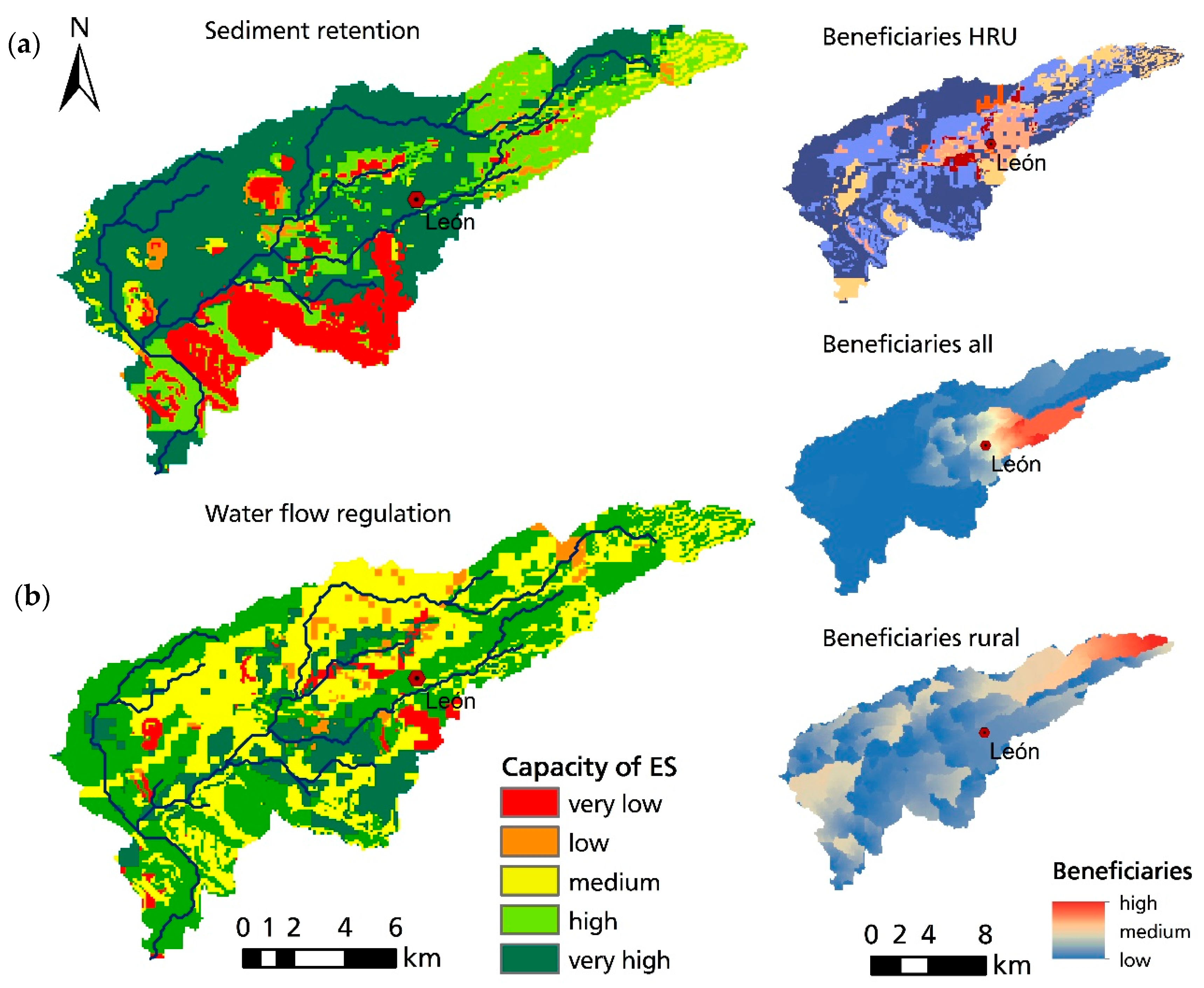
Figure 5.
Modelling results of the RIOS Investment Portfolio Adviser.
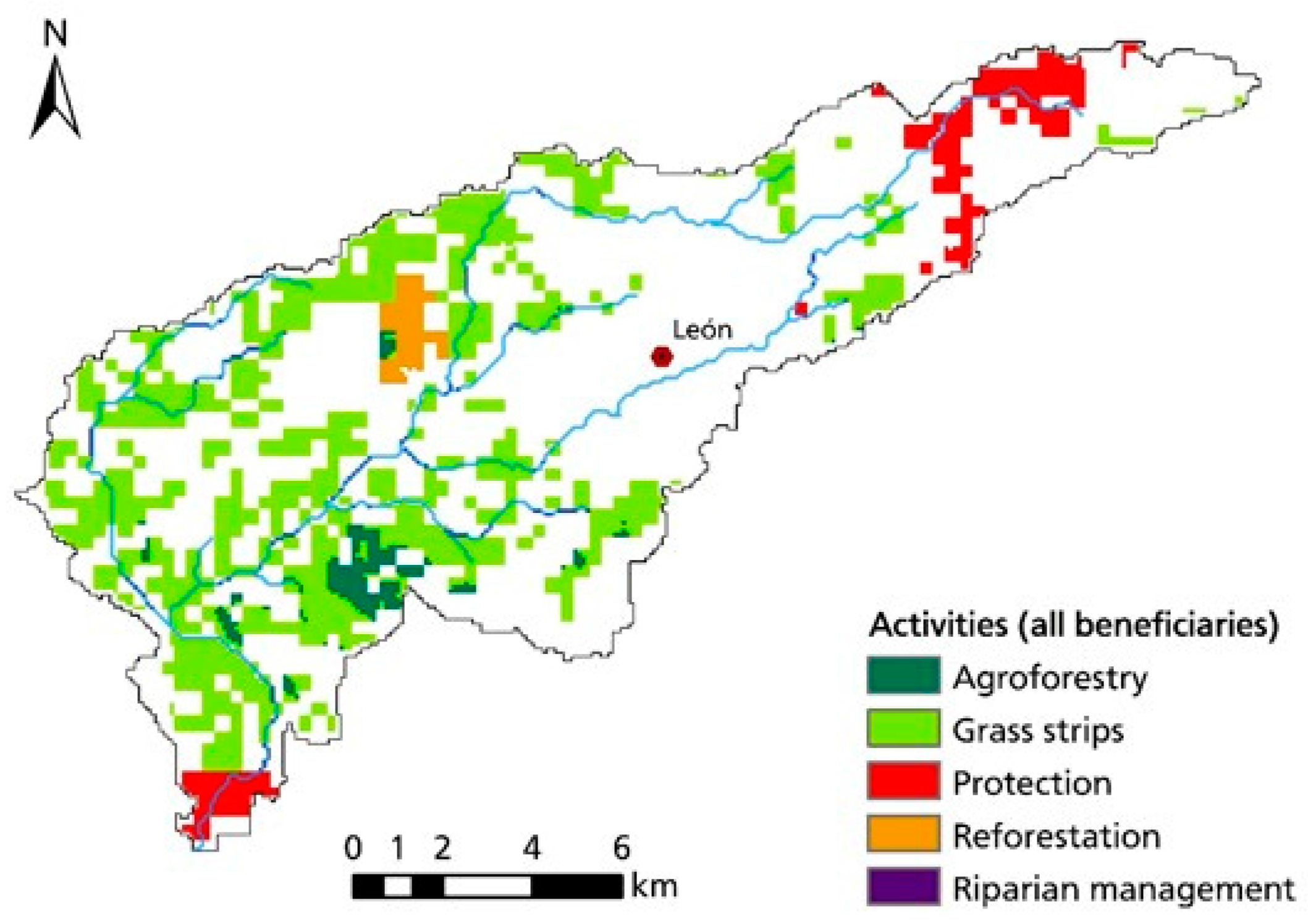
Figure 6.
Modelling result of the RIOS Portfolio Translator showing land use changes from base line scenario to (->) transitioned land use scenario (implemented land use change activities) on a pixel by pixel basis. Suggested areas for protection (pixels in red in Figure 5) remain with the land use of the base line scenario and do not appear in Figure 6.

Figure 7.
Modelling results of RIOS evaluated with the InVEST water yield model. (a): Baseline; (b): transitioned; (c): Unprotected.
Figure 7.
Modelling results of RIOS evaluated with the InVEST water yield model. (a): Baseline; (b): transitioned; (c): Unprotected.

Figure 8.
Output of the InVEST Water Yield Model. (a): Water yield per subwatershed; (b): Water consumption; (c): Water supply per subwatershed.
Figure 8.
Output of the InVEST Water Yield Model. (a): Water yield per subwatershed; (b): Water consumption; (c): Water supply per subwatershed.
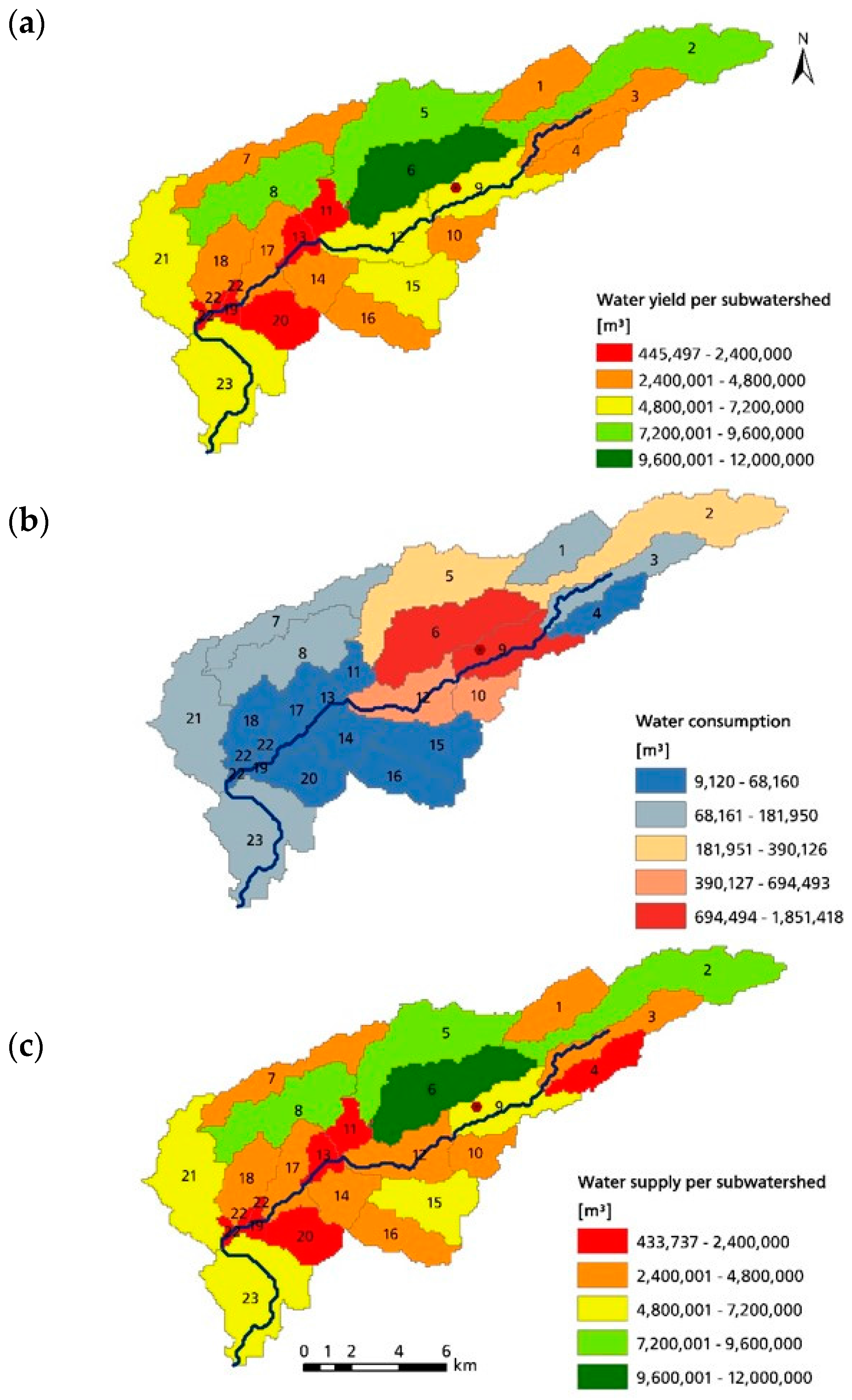
Figure 9.
Output of the InVEST SDR Model. (a): Sediment export; (b): Sediment retention.
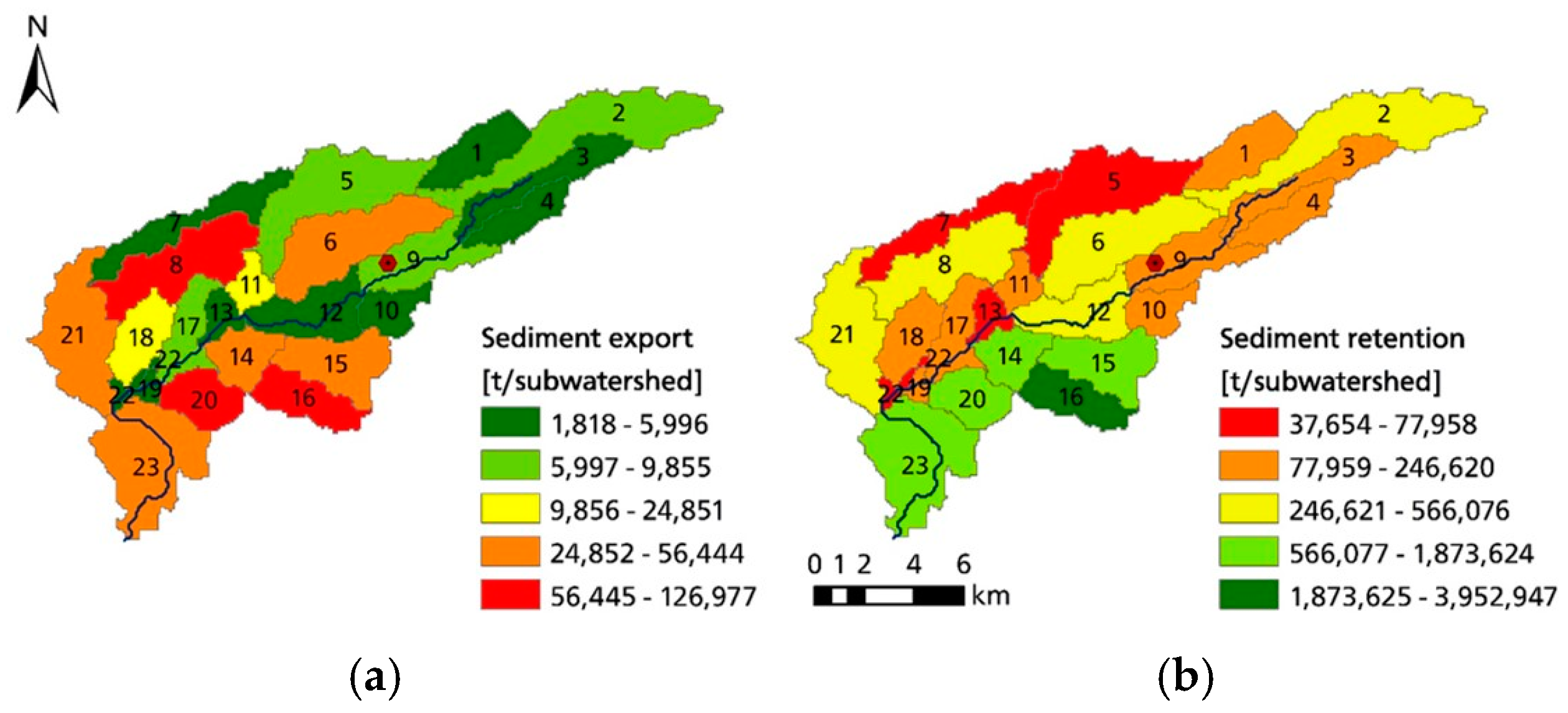
Figure 10.
Results of RIOS evaluated with the InVEST SDR model. (a): Baseline; (b): transitioned; (c): Unprotected.
Figure 10.
Results of RIOS evaluated with the InVEST SDR model. (a): Baseline; (b): transitioned; (c): Unprotected.

Figure 11.
Possible iterative combination of models.

Table 1.
Model input data specification.
| Data Type (Format) | Source | Resolution | Required for |
|---|---|---|---|
| Biophysical inputs | |||
| Digital elevation model (raster) | USGS HydroSHEDS [23] | 3 arc-seconds → approx. 90 m at equator | InVEST, RIOS, SWAT |
| Land use/land cover (raster) | GlobCover 2009 [24] | 300 m | InVEST, RIOS, SWAT |
| Weather data (gages) | Data from NCEP for 1979–2014 [25] | 2 weather stations | SWAT |
| Soil data (raster and database) | HWSD, [26] | 30 arc-seconds → approx. 1 km | InVEST, RIOS, SWAT |
| Average annual rainfall (raster) | WorldClim, annual average from 1960–1990 [27] | 30 arc-seconds → approx. 1 km | InVEST, RIOS |
| Mean annual actual evapotranspiration (raster) | CGIAR-CSI, annual average from 1950–2000 [28] | 30 arc-seconds → approx. 1 km | RIOS |
| Socio-economic input | |||
| Location & number of beneficiaries (raster) | Calculated with population density [16] | Municipality León | RIOS |
| Per capita water consumption (table) | FAO Aquastat data [17] | Annual average for Nicaragua | InVEST |
Table 2.
Variables to represent the selected HES [40].
Table 2.
Variables to represent the selected HES [40].
| Ecosystem Service Modelled | Variables of the HRU Output File | |
|---|---|---|
| Variable Name | Definition | |
| Water flow regulation | SW_END | Soil water content (mmH2O) at the end of the time period |
| SURQ_CNT | Surface contribution (mmH2O) to streamflow in the main channel during time step | |
| LATQ_GEN | Lateral flow generated in the HRU during time step (mmH2O) | |
| GW_Q | Groundwater contribution to streamflow (mmH2O), also called base flow | |
| Sediment retention | SYLD | Sediment yield transported into the main channel during time step (t/ha) |
Table 3.
Results of model comparison.
| Point of Comparison | SWAT | RIOS | InVEST |
|---|---|---|---|
| Model description | Hydrologic model with different output variables | Implementation of activities to maintain, protect or restore ES | Different models for final and supporting ES used: Water Yield and SDR Model |
| Inclusion of beneficiaries | Cannot be included directly Visual comparison possible | Beneficiaries-raster to weight activity areas | Water yield model uses water demand table |
| Uncertainty | Calibration and valuation possible but for study area no calibration | No option for calibration; comparison of input data with literature values | Calibration possible with sediment load or stream flow but for study area no calibration |
| Data requirements & pre-processing | High data requirement and pre-processing | Medium data requirement and high pre-processing | Medium data requirement and low pre-processing |
| Training effort | Training effort high | Training effort medium to high | Training effort medium |
| Time requirement | High | Medium | Low to medium |
© 2018 by the authors. Licensee MDPI, Basel, Switzerland. This article is an open access article distributed under the terms and conditions of the Creative Commons Attribution (CC BY) license (http://creativecommons.org/licenses/by/4.0/).
Share and Cite
MDPI and ACS Style
Lüke, A.; Hack, J. Comparing the Applicability of Commonly Used Hydrological Ecosystem Services Models for Integrated Decision-Support. Sustainability 2018, 10, 346. https://doi.org/10.3390/su10020346
AMA Style
Lüke A, Hack J. Comparing the Applicability of Commonly Used Hydrological Ecosystem Services Models for Integrated Decision-Support. Sustainability. 2018; 10(2):346. https://doi.org/10.3390/su10020346
Chicago/Turabian StyleLüke, Anna, and Jochen Hack. 2018. "Comparing the Applicability of Commonly Used Hydrological Ecosystem Services Models for Integrated Decision-Support" Sustainability 10, no. 2: 346. https://doi.org/10.3390/su10020346
Note that from the first issue of 2016, this journal uses article numbers instead of page numbers. See further details here.