Economic Decision-Making for Coal Power Flexibility Retrofitting and Compensation in China


1
School of Physics & Electronic-Electrical Engineering, Ningxia University, Yinchuan 750021, China
2
School of Economics and Management, North China Electric Power University, Beijing 102206, China
3
Beijing Key Laboratory of New Energy and Low-Carbon Development, North China Electric Power University, Changping, Beijing 102206, China
*
Authors to whom correspondence should be addressed.
Sustainability 2018, 10(2), 348; https://doi.org/10.3390/su10020348
Submission received: 2 November 2017
/
Revised: 26 January 2018
/
Accepted: 26 January 2018
/
Published: 29 January 2018
(This article belongs to the Section Energy Sustainability)
Abstract
:In China, in order to integrate more renewable energy into the power grid, coal power flexibility retrofitting is imperative. This paper elaborates a generic method for estimating the flexibility potential from the rapid ramp rate and peak shaving operation using nonlinear programming, and defines three flexibility elastic coefficients to quantify the retrofitted targets. The optimized range of the retrofitted targets determined by the flexibility elastic coefficients have a reference significance on coal power flexibility retrofitting. Then, in order to enable economic decisions for coal power flexibility retrofitting, we address a profit maximizing issue regarding optimization decisions for coal power flexibility retrofitting under an assumption of perfect competition, further analyzing the characteristic roots of marginal cost equal to marginal revenue. The rationality of current compensation standards for peak shaving in China can also be judged in the analysis. The case study results show that economic decision-making depends on the compensation standard and the peak shaving depth and time. At a certain peak shaving depth and time, with rational compensation standard power plants are willing to carry out coal power flexibility retrofitting. The current compensation standard in Northeast China is high enough to carry out coal power flexibility retrofitting. These research conclusions have theoretical significance for China’s peak shaving compensation standards formulation.
1. Introduction
China has faced at severe curtailment of renewable energy in recent years, but flexible power resources, such as gas generators and pumped storage power stations, are seriously short. The total installed capacity of these two kinds of flexible power was still lower than 6% by the end of 2016 [1]. In a short period of time, their installed capacity is difficult to achieve at a certain scale to bear flexible electricity requirements. In the face of severe renewable energy curtailments, due to the country’s resource endowment and the surplus of coal power installed capacity [2], to rely on coal power flexibility retrofitting as flexible resource is imperative.
Research on thermal power flexibility retrofitting mainly includes five aspects: the first is peak shaving depth retrofitting with straight condensing units, the second is ramp rate retrofitting with straight condensing units, the third is the rapid start–stop of thermal power units, the fourth is the thermoelectric decoupling of combined heat and power units (CHP), and the fifth is flexible boiler fuel retrofitting. However, this paper only studies the first two aspects. The entire retrofitting process and technical details are shown in Table 1.
A number of power system flexibility researchers have investigated how to define power system flexibility and flexibility metrics [3,4,5,6], how to evaluate it [7,8,9,10,11,12,13,14] and which resources can provide flexibility [15,16]. Basically, the flexibility resources focus on demand side resources [17,18,19], energy storage [20,21,22,23], advanced energy conversion technologies [24,25], and so on. Andresen (2012) et al. used a Fourier-like decomposition of residual load to estimate flexibility requirements [26]. Shu (2017) et al. focused on thermal unit transformation, power system interconnection and demand-side management to solve China’s renewable energy accommodation [27]. There is little research in the literature on power system flexibility provided by thermal power retrofitting, especially the retrofitted ramp rate and peak shaving depth.
Marginal revenue and marginal cost are elements of the classic theory of Western economics. They are also used in analyzing related issues in the power sector. Kuang (2008) et al. researched the compensation standard of interruptible load in China’s power market [28]. Jia (2007) et al. researched the contract effect on the stability of the power market with the help of characteristic roots [29]. Liu (2007) pointed out that in the power market, generation companies must participate in market competition according to the equation of marginal cost and marginal revenue [30]. There is no literature research on economic decision-making for coal power flexibility retrofitting with marginal cost and marginal revenue.
This paper elaborates a generic method based on residual load to estimate the flexibility potential provided by the retrofitted ramp rate and peak shaving depth, further addressing a profit maximizing issue regarding the optimization decision for flexibility retrofitting in coal power plants under an assumption of perfect competition and the rationality of current compensation standards with the help of characteristic roots. The paper is organized as follows: base on an IEEE (Institute of Electrical and Electronics Engineers) 10 unit and 39 node system, Section 2 reviews flexible operation in a power system, then Section 3 describes the flexibility potential model of ramp rate retrofitting, then calculates the upward flexibility potential; Section 4 describes the flexibility potential model of peak shaving depth retrofitting, then calculates the downward flexibility potential. In these two sections, three elastic coefficients are defined to quantitatively describe the optimized range of the retrofitted targets. The flexibility cost and revenue provided by peak shaving depth retrofitting are presented in Section 5, whereas the characteristic root analysis with the equation of marginal revenue and marginal cost is shown in this section. Finally, Section 6 summarizes the conclusions.
2. Flexible Operation in a Power System
Renewable energy is currently prioritized for integration, meaning that coal power plants must provide more flexible output to keep the available energy at the required level in the grid. Some coal power units are designed to ramp up and down rapidly in short periods of time to provide flexible electricity to fill the gaps in grid output caused by renewable energy’s intermittency, as shown in Figure 1. The dotted lines are residual load curves before being retrofitted, and the solid lines are residual load curves after being retrofitted. As a result of coal power retrofitting, coal power units can rapidly respond to renewable energy’s intermittency and promote renewable integration. Then the calculation models of a single unit’s flexibility potential are designed in the following two sections.
3. Flexibility Provided by Rapid Ramp Rate
3.1. Model for Flexibility Potential Provided by Rapid Ramp Rate Retrofitting
To provide reliable backup for renewable energy integration, coal power units respond more quickly to increasing and providing flexible electricity when renewable energy is insufficient. This is named upward flexibility. Some existing units do not have the ability of a rapid ramp for short periods of time, and they need to be retrofitted. The output curves before () and after () ramp rate retrofitting are shown in Figure 2. The shaded areas represent the flexible electricity Etu.
In Figure 2, represents the initial output power before the unit response to rapid ramp, as there are more electricity demand gaps in the grid caused by renewable energy intermittency, thermal power units begin to rapidly ramp up in a short period of time, which is response time . Due to the fact that the unit may not reach the rated output in the specified time , there are different models for different response times. respectively represent the upward ramp rate before and after being retrofitted, and respectively represent the time arriving at the rated output before and after retrofitting. From , time starts.
When , the upward flexible electricity is:
When , the upward flexible electricity is as follows.
When , the upward flexible electricity is:
Theoretically, it is possible for , but in practice considering the current technical level it is impossible. However, for the integrity of the model, we retain Equation (3).
3.2. Ramp Rate Retrofitting Scenario and Flexibility Potential
According to the Renewable Energy Outlook 2016 [31], the ramp rate for an inflexible unit is 0.6–4% per minute of rated power; and the ramp rate for a flexible unit is 4–11% per minute of rated power.
There is a parameter list for an IEEE 10 unit and 39 node system (Table 2).
Basically, it can be used to simulate an actual power system with other generation resources. The scale of a power system with ten units and other power generation units is appropriate, as it will not lead to a large amount of calculation and analysis. Their ramp rates in the list are all in the range of 0.6–4% per minute of rated power, so they are all inflexible units. Now they are all retrofitted in order to rapidly respond to supply flexible electricity.
From the original ramp rate in Table 2, the larger units have a higher percentage of ramp rates, except for the 350 MW unit. Since 2007, China has implemented the policy strategy of substituting large units for small units, because the larger units have high parameters, high efficiency and low emission. Thus, assuming that the larger the unit is, the higher the ramp rate is, after ramp rate retrofitting, the ramp rate of 350 MW unit is 4–8% per minute of rated power; that of the 600 MW unit (including three units of 608 MW, 640 MW and 660 MW) is 5–9%; that of the 700 MW unit (including two units of 750 MW,732 MW) is 6–10%; that of 930 MW unit is 7–11%; and that of the 1000 MW unit (including two units of 1145 MW and 1100 MW) is 8–12%. One retrofitted target value represents one scenario, in order to describe the range of clearly, we use as the retrofitted target in every scenario; all of the scenarios are set and shown in Table 3.
Due to flexible electricity always trading in 15 min, the flexible electricity is also calculated in 15 min for all scenarios. Now what are the maximum values of in 15 min for these ten units? Those are the maximum upward flexible electricity. The model is as follows:
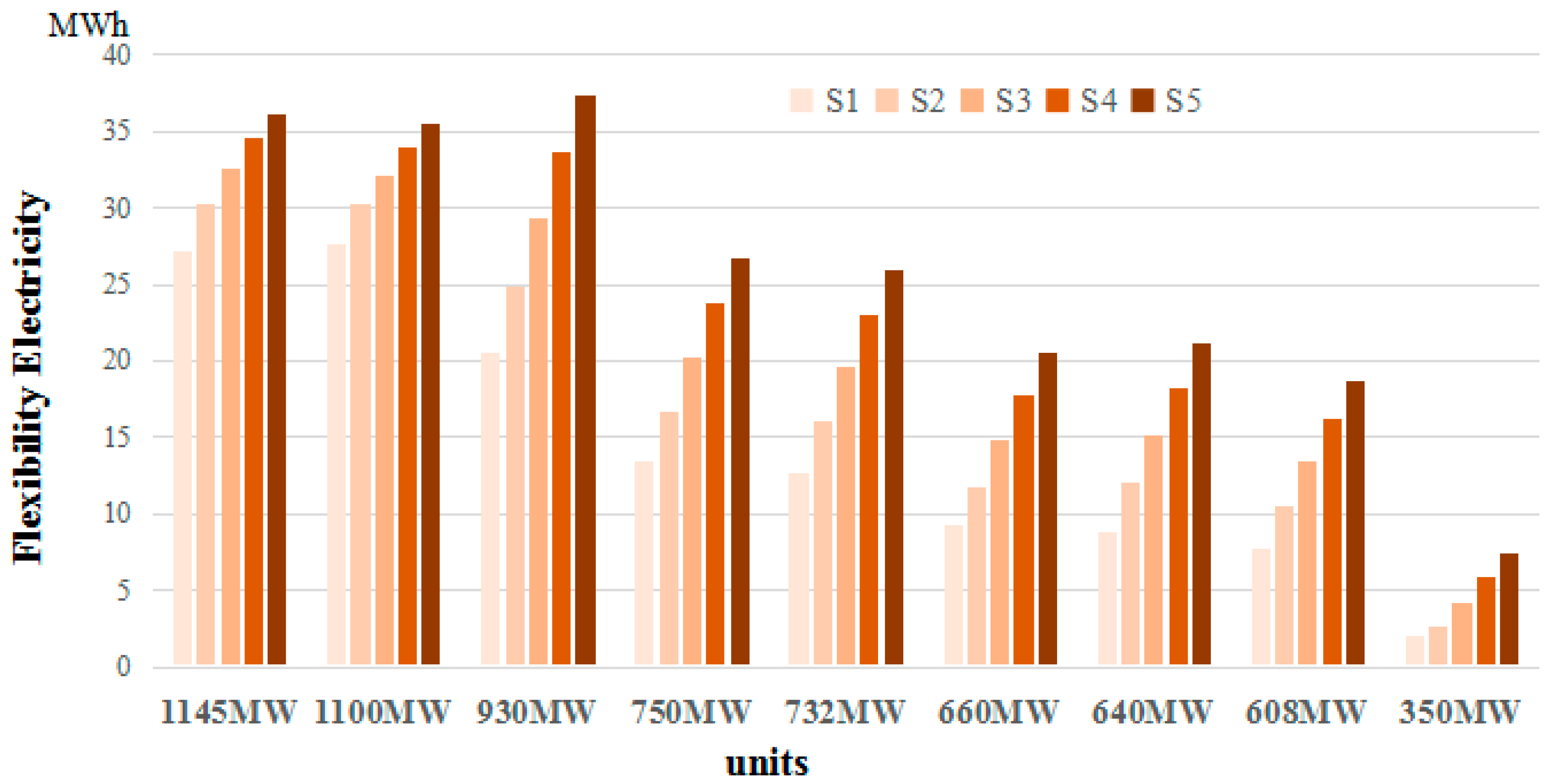
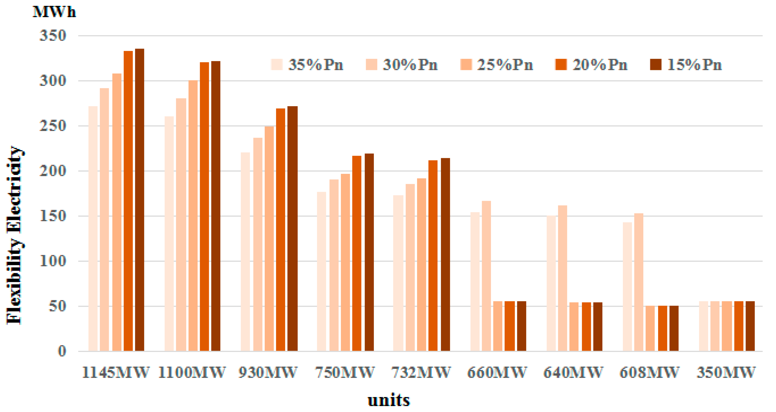
From Equations (1) and (2), the function is a nonlinear function. Therefore, calculating the maximum value of requires typical nonlinear programming. We have combined quantitative analysis and scenario analysis in this subsection. Take Equation (2) as an example, as equals 15 min and is a known quantity for every unit, then is a function of two variables with and . To calculate the maximum flexible electricity, is in a three-dimensional space. After we set scenarios according to different , in a certain scenario, equals , and will become a function of one variable , then to calculate the maximum flexible electricity of will be in the plane of and . The calculation in a plane is easier than in a three-dimensional space. is the quadratic function of , and this quadratic function curve opens down, so has only one maximum value in the range of . The quadratic function curve of opens up, so has only one minimum value in the range of . We can call one nonlinear programming function ‘fmincon’ of MATLAB and calculate all the maximum values with different scenarios. Thus, based on nonlinear programming, select as a choice variable, in the five scenarios the highest upward flexible electricity of each unit is shown in Figure 3. In order to make the highest upward flexible electricity look regular, we rank the upward flexibility electricity of five scenarios from a large scale unit to a small scale unit.
Only the 350 MW unit cannot reach the rated output in 15 min, the other units can achieve maximum output, therefore its flexibility potential is a bit lower. For other units, the greater the rated output, the greater the retrofitted ramp rate, and also the greater the flexible electricity.
In economics, elastic coefficients are often used to describe some dependent relationships of the growth amplitude of one variable to the increase of another variable in a certain period time. In order to quantitatively describe the change law of upward flexibility with the change of retrofitted ramp rate, the upward elastic coefficient eup of ramp rate retrofitting can be defined as:
where is the increased upward flexible electricity corresponding to two adjacent scenarios in 15 min, equals to the increased ramp rate of two adjacent retrofitted ramp rate targets, two adjacent scenarios are the scenario of S2 and S1, S3 and S2, and so on. equals to 15 min, and is the increased output power of two adjacent scenarios within 15 min. All the elastic coefficients are shown in Table 4.
Obviously the rule “the bigger the better” does not apply to the retrofitted ramp rate, but the greater the elasticity coefficient, the better the ramp rate, and the greater the increased upward flexible electricity. The optimized ramp rate should between the range that has the maximum upward flexibility elastic coefficient and the optimized range of the ramp rate can be a reference for the retrofitted ramp rate.
The optimized ramp rate for a 600 MW unit is 6–7% per minute, those for a 700 MW and 900 MW unit are 7–9% per minute, and the optimized ramp rate for 1000 MW unit is 8–9% of the rated output per minute.
4. Flexibility Provided by Peak Shaving Depth Retrofitting
4.1. Model for Flexibility Potential Provided by Peak Shaving Depth Retrofitting
To provide flexible electricity and ensure renewable energy curtailment less, when power load demand is low, coal power units response more quickly to ramp down and reduce the output power. It is named downward flexibility.
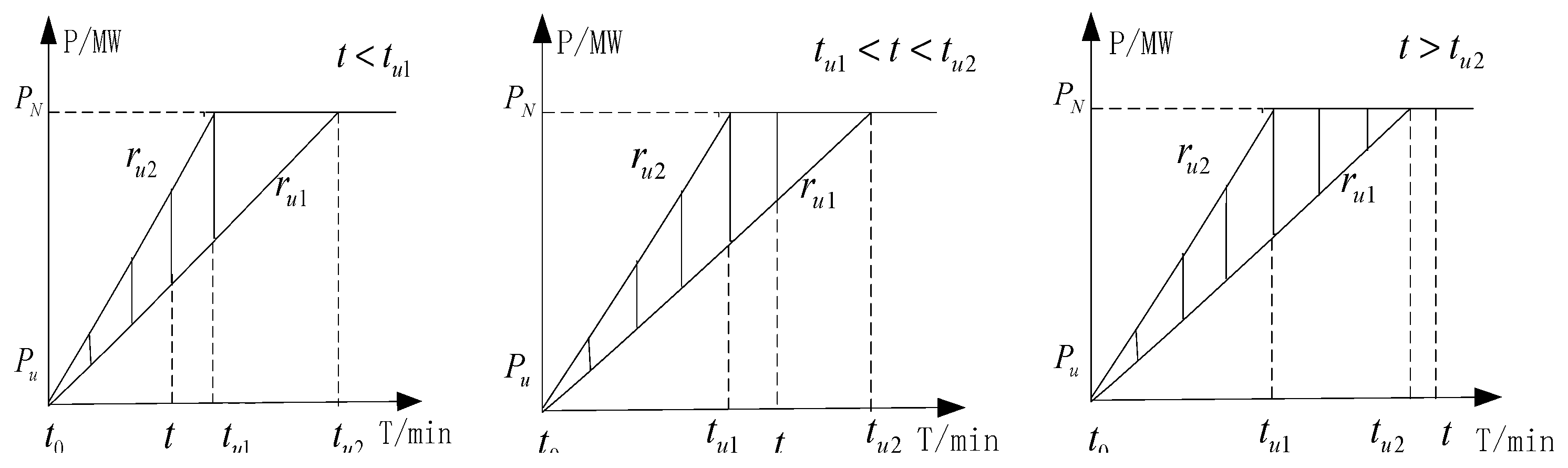
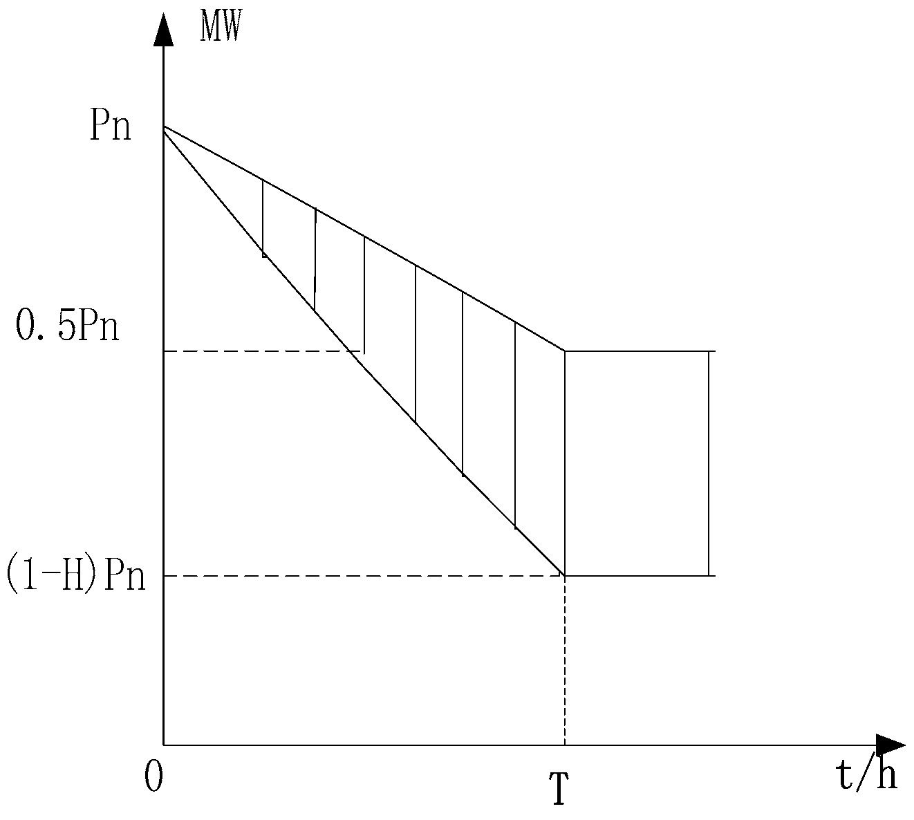
In general, a coal power unit is divided into two kinds of units, one is a straight condensing unit that is not used to being a heating unit, the other is an extraction condensing unit that is always used as a heating unit. At present, the peak shaving operation capability for a straight condensing unit in actual operation is generally about 50% of the rated capacity, this means that its output power in peak shaving operation is from the rated power to 50% of the rated power. For a typical extraction condensing unit in a heating period, it is only about 20% of rated capacity in China; this means that its output power in peak shaving operation is from the rated power to 80% of the rated power in order to ensure that enough heat can be supplied. Through coal power flexibility retrofitting, it is expected that the peak shaving depth of a straight condensing unit can be increased by 15–20% of the rated capacity, with its minimum technical output reaching 30–35% of the rated capacity, meaning that the peak shaving depth is 0.65–0.70. It is also expected that the depth of the extraction condensing unit can be increased by 20% of the rated capacity, with its minimum technical output reaching 40–50% of the rated capacity, meaning that the peak shaving depth is 0.50–0.60. The generation output curves before and after retrofitting are shown in Figure 4.
In the models, respectively represent the minimum technical output before and after depth retrofitting, represents the initial output power before response to the peak shaving operation, represent the running time to reach and , respectively. Time starts from . The shaded area is the downward flexible electricity .
When , the downward flexible electricity is:
When , the downward flexible electricity is:
When , the downward flexible electricity is:
In the models, if , all the model expressions also can be applied. Theoretically, it is possible for , but in practice considering the current technical level it is impossible. For the integrity of the model, we retain Equation (8).
4.2. Flexibility Potential for Peak Shaving Depth Retrofitting
In order to get the best flexibility potential in a short period of time, both the peak shaving depth and downward ramp rate need to be retrofitted. In the following two subsections, the flexibility potential for the peak shaving depth will be divided into two cases to analyze. One case is set as the unified downward ramp rates and five different depths. The other case is set as the same depth and four different downward ramp rates.
4.2.1. Unified Downward Ramp Rate and Five Different Depth
According to Danish technology experience, the retrofitted minimum output of a coal power unit is around 20% of the rated power. According to on-the-spot survey results in a coal power plant in China, the designed minimum output power is 20% of the rated output power for many new coal power units, in order to mine the maximum flexibility potential we assume that the minimum retrofitted depth in China is 15% of the rated power.
In this subsection, we set up five different retrofitted depths, shown in Table 5, where equals . The downward ramp rates are a unified set and are also shown as the third column in Table 5: the downward ramp rate of 300 MW unit is 4% of rated power per minute; that of 600 MW unit is 5% per minute; that of 700 MW unit is 6% per minute; that of 900 MW unit is 7% per minute; that of 1000 MW unit is 8%. All of the operation times td1 are also shown in Table 5.
Most of the running times are shorter than 15 min, only the running time identified with * is longer than 15 min; they will be fitted for different calculations of Equations (6) and (7). Then the maximum downward flexibility can be calculated with the following model:
Using the same analysis as for upward flexibility , all the downward flexibilities are calculated with as the choice variable and shown in Figure 5. According to Figure 5, the larger the rated output, the greater the flexible electricity.
With the increasing , the flexible electricity will decay quickly. For a 350 MW unit, due to being longer than 15 min, Equation (6) has nothing to do with the minimum output, so the potential flexibility is the same at all different depths. In order to quantitatively describe the change law of downward flexibility with the change of retrofitted depth, the peak shaving elasticity coefficient is defined as follows:
where is equal to the increased retrofitted minimum output power of two adjacent scenarios for every unit, is the increased flexible electricity of two adjacent scenarios within 15 min. All the elastic coefficients are shown in Table 6.
According to Table 6, the best retrofitted depth for these ten units is in the range of 20–25%Pn. Due to the increasing generation loss with peak shaving operation, the depth is not subject to the rule “the deeper the better”, but the greater the peak shaving elasticity coefficient, the better the corresponding depth. The range of the optimized depth can be a reference for the retrofitted depth.
4.2.2. Same Depth and Four Different Downward Ramp Rates
In this section, we set the retrofitted depth as 20% of the rated power and the downward ramp rate in four scenarios, as follows:
- for 300 MW unit; for 600 MW unit;
- for 700 MW unit; for 900 MW unit;
- for 900 MW unit.
This is like an upstairs, so we name it upward ladders and use another notion to represent it in order to describe the range of clearly. Four scenarios are shown in Table 7.
All of and the running time are shown in Table 8.
According to Table 8, is longer than 15 min only for the 300 MW and 600 MW units, for the other units it is less than 15 min, they are also fitted for different Equations, namely (6) and (7). The maximum downward flexibility can be calculated by the following model:
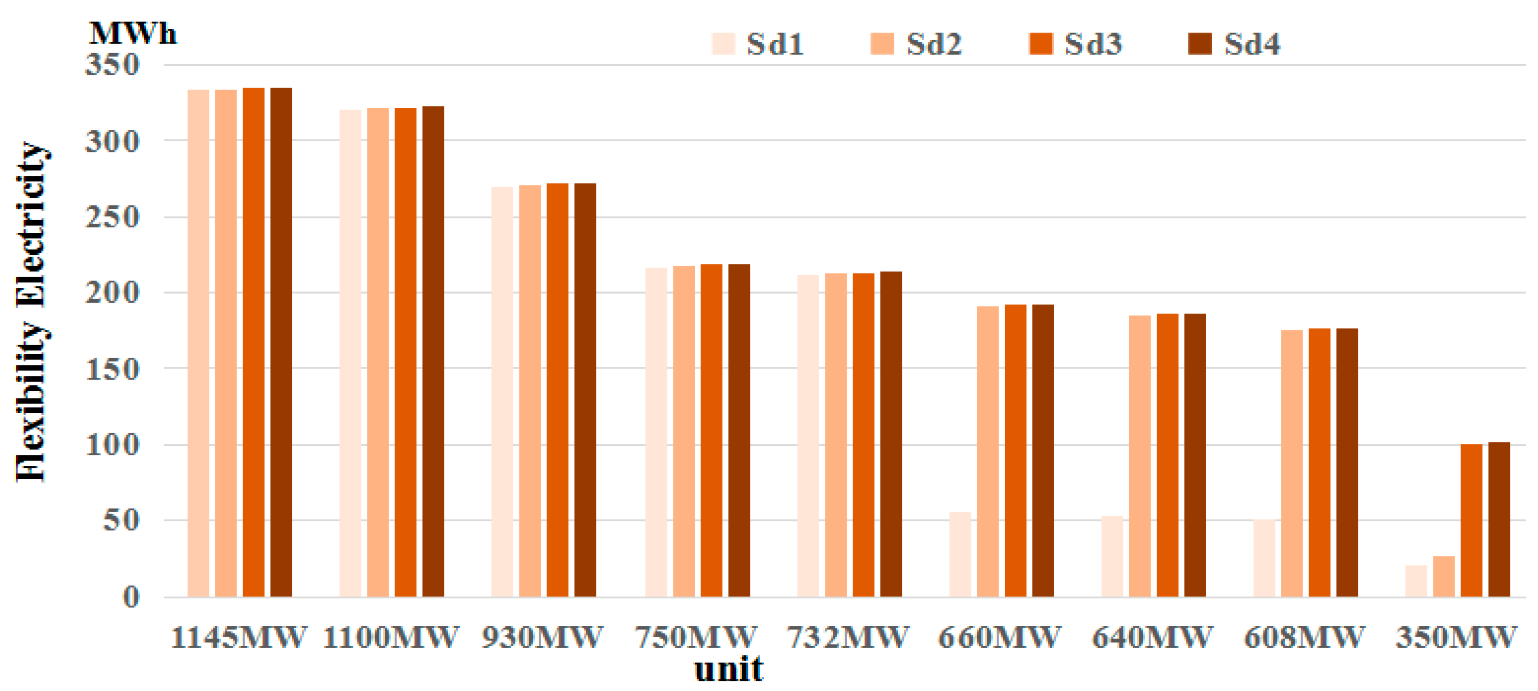
As for the analysis of upward flexibility , all the maximum flexible electricity values are calculated with as the choice variable and shown in Figure 6.
According to Figure 6, the greater the ramp rate, the greater the flexible electricity, but the growth rate of flexible electricity is far less than that of the corresponding ramp rate. In order to quantitatively describe the change law of downward flexibility with the change of the retrofitted downward ramp rate, the downward elastic coefficient is defined as:
where is the increased flexible electricity of two adjacent retrofitted within 15 min, equals the increased ramp rate of two adjacent , that is for every unit. All downward elastic coefficients are shown in Table 9. There are some occasional high values, and for one unit there is one occasional high value, it represents that with the same change of retrofitted , it is the range of retrofitted ramp rate with the highest flexible electricity. The range can be used as a reference value for the optimized downward ramp rate.
Obviously, the downward ramp rate is not subject to the rule “the sooner the better”, but the larger the downward elastic coefficient, the better the corresponding ramp rate.
5. Economic Decision-Making for Coal Power Flexibility Retrofitting
In this section, we address a profit maximizing issue regarding the optimization decision for coal power flexibility retrofitting under an assumption of perfect competition.
The flexibility retrofitting marginal cost of a generating enterprise refers to the increased flexibility costs in the total electricity caused by per unit of increased flexible electricity. The flexibility electricity marginal revenue refers to the total revenue increment brought by per unit deal of increased flexible electricity.
As the flexible electricity marginal revenue is greater than its marginal cost, power generation enterprises are profitable, and coal power flexibility retrofitting is feasible; once the marginal cost is greater than the marginal revenue, thermal power flexibility retrofitting is unfeasible. It can be used to judge whether or not the plant operators are willing to carry out coal power flexibility retrofitting, and can also be used to judge the rationality of current compensation standards in China.
The flexibility requirement has two aspects, an upward flexibility and a downward flexibility requirement. For upward flexibility, the greater the upward ramp rate, the sooner the power output is close to the rated output, and the greater the generation electricity. The ability to ramp up quickly may have extra value to the system beyond just the extra electricity generated. However, in this section we only research the flexible electricity marginal cost and marginal revenue provided by peak shaving depth retrofitting.
Flexible electricity () increases with increased depth, and is a function of peak shaving depth (); flexible electricity cost () is also a function of flexible electricity (), so the cost also can be expressed as a function of the depth. Therefore, the flexibility marginal cost (MC) can be expressed as:
Power enterprises reduce their power trading through downward load operation, therefore the flexible electricity revenue () is the compensation for peak shaving operation, it can be expressed as a function of flexible electricity (). By the same token, flexible electricity revenue is also a function of the depth (H), so flexibility marginal revenue (MR) can be expressed as:
5.1. Fixed Cost of Peak Shaving Depth Retrofitting
For the fixed cost of peak shaving depth retrofitting, detailed economic indicators need to be clarified gradually in the demonstration pilot project, now there are no official statistics. Thus, according to the prophase research results from National Energy Administration, the per unit of flexibility retrofitting cost is commonly between 50 yuan/kW and 200 yuan/kW [33]. Taking a 600 MW unit as an example, if the designed minimum output power is 50% of the rated power, we set the scenarios according to different depths with different costs. These are shown in Table 10.
From Table 10, the retrofitting cost per MW increases with the increase in depth, because each boiler has a designed lowest stable-combustion depth, if the designed depth is deeper than the running depth, the only retrofitting process is to ensure the normal working of the environmental protection equipment; if it is higher than the running depth, the retrofitting process will become complicated in order to ensure the stable combustion of the boiler and the normal working of the environmental protection equipment.
To estimate with the quadratic function, then the function between and is:
This is the total retrofitting cost. If the unit can serve years after retrofitted, and the rate of return on investment is , then the annual cost will be ; if the total time of annual peak shaving operation is , then the average fixed cost of one time peak shaving operation will be:
where is the capital recovery factor. Assuming that in the electrical power investment, equals 8%, and the service life of coal power units after being retrofitted is 15 years, then the capital recovery factor equals 0.1168. Then the average fixed cost of one time peak shaving operation will be:
5.2. Variable Cost-Generation Loss Cost from Peak Shaving Depth Retrofitting
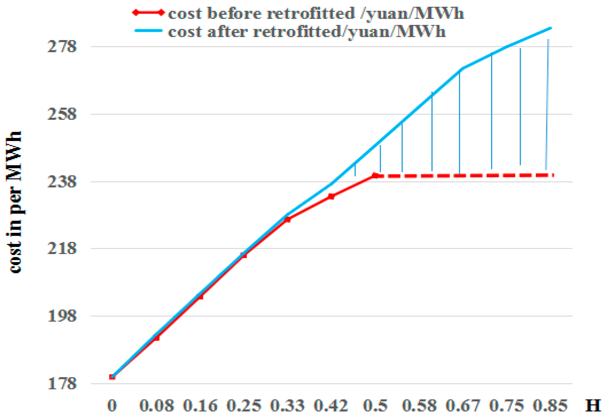
Peak shaving depth retrofitting inevitably leads to increasing generation losses. Also taking the 600 MW unit as an example, assuming that the generation heat rate with different active powers before retrofitting is shown in Table 11 (the depth is from 0 to 50%). The generation heat rate after retrofitting is set according to Germany’s experience [34] and shown in Table 11. Assuming that the price of standard coal (5500 kCal/kg) is 600 yuan/ton, the per unit generation cost is also shown in Table 11.
Before retrofitting, the function between per unit generation cost and the depth can be fitted using the least square method with Equation (18).
After retrofitting, the function between per unit generation cost and the depth can be fitted as follows:
The generation loss cost of per unit is shown in Figure 7 by a shaded area.
If flexible electricity is , the total generation loss cost is:
The total retrofitting cost for one time peak shaving operation should include both the fixed cost and the variable cost. Because the unit of is , the unit of is yuan. After unifying the units of the two kinds of cost, the unit of the total cost is 106 yuan.
Therefore, the total cost for one time peak shaving operation is:
5.3 Revenue from Peak Shaving Depth Operation
According to the Northeast Regional Electricity Market Operation Rules issued by the Northeast NEA [35], for units with a peak shaving operation, if the depth is higher than 40%, the subsidy for per megawatt hour electricity is 1000 yuan, and if the depth is lower than 40%, the subsidy is 400 yuan, then two scenarios for the compensation standard of per megawatt hour electricity, basic scenario () and policy scenario (), are shown in Table 12.
According to these two compensation scenarios, the functions between per unit flexible electricity revenue can be expressed as the piecewise function and , respectively. Both of these are always constant in every piecewise range of .
If the flexible electricity of the peak shaving operation is , the per unit flexible electricity revenue is , the flexibility revenue will be , that is, .
5.4. Flexible Electricity Marginal Cost and Marginal Revenue
We simplified the flexibility potential model of the peak shaving depth retrofitting in Figure 4, this is shown in Figure 8.
According to Figure 8, the total flexible electricity is as follows:
If a 600 MW unit operates downward from the rated power to (1-H) times of the rated power, the flexible electricity is , therefore , and the for these three scenarios is Equation (23).
where , because is equal to or in different scenarios, they are all constant in every piecewise range of , so all in two scenarios is always equal to zero.
The flexible electricity marginal cost for those two scenarios is found by Equation (24).
5.5. Analysis of Characteristic Roots in Two Scenarios
In economic terms, when , the producers can profit from this transaction and they are willing to continue production and transaction. In power economics, only when coal power plants can benefit from peak shaving operations are they willing to carry out coal power flexibility retrofitting. This means that only when the margin revenues from the peak shaving operation can cover the marginal cost of coal power flexibility retrofitting, are the operators are willing to carry out coal power flexibility retrofitting.
Due to the fact that electricity trading is always in 15 min, we set the response time T = 0.25 h, 0.50 h, 0.75 h, 1 h, where h equals to one hour, thus the inequality of is as follows:
As we know, it is difficult to predict the times of peak shaving operation , as it depends on the wind speed, the changes of power load and other factors in the power system. However, the maximum annual operation hours of coal power units is 5500 h, if the maximum equals 5500, then the minimum of will equal 0.0002; is far less than the minimum of and (the minimum of is 0.0004 in the range of ), in this case the inequality of is simplified as follows:
The characteristic roots of the inequality of can reflect the range in which the margin revenue can cover the margin cost with a certain . For coal power units, which can only run with the depth at which the margin revenue can cover the margin cost, the plant operators are willing to participate in peak shaving operation. The characteristic roots for different are always . This is related to the compensation standard and the times of peak shaving operation. If there are characteristic roots in the range of , then all of the ranges of and the total annual running hours in two scenarios are show in Table 13 and Table 14.
In the basic scenario, the maximum annual peak shaving running hours is 402, as the depth is 0.85; in the policy scenario, the maximum annual peak shaving running hours is 322, as the depth is 0.85.
In fact, in 2016, the most serious wind power curtailment was in four provinces [36]: Gansu, Xinjiang, Inner Mongolia, and Jilin, and the curtailment rate was 43%, 38%, 21% and 30%, respectively. Among them, the curtailed wind power and the total flexibility retrofitting capacity of coal power units in Jilin province [37] are show in Table 15, and we can roughly estimate the peak shaving running hours, also shown in Table 15.
From Table 15 we can see that if all of the curtailed wind power is integrated by the peak shaving operation of the total coal power flexibility retrofitting units from , then the total peak shaving running hours will be 2180 h when the depth is from 0.50 to 0.60, and the total peak shaving running hours will be 727 h when the depth is from 0.50 to 0.85. These are all bigger than the calculated running hours in Table 13 and Table 14. This means that in the north areas where the curtailed wind power needs to be integrated through coal power peak shaving operations, the actual times should be greater than or equal to the calculated in Table 13 and Table 14.
If we roughly set the total times of peak shaving operations as 100, 300 or 500, then the characteristic roots for in these two scenarios are shown in Table 16.
From Table 16 we can see that the characteristic roots have a relationship with the compensation standard and the times of peak shaving operation. There are three cases for the characteristic roots:
- (1)
- If there is a characteristic root in every piecewise range of , the peak shaving retrofitting decision will be ‘yes’. As the actual running depth is less than or equal to the calculated in every piecewise range of , the margin revenue can cover the margin cost, and the compensation standard is rational and the plant operators are willing to carry out coal power flexibility retrofitting.
- (2)
- If there are no roots in every piecewise range of and the calculated is bigger than every piecewise range of , then the peak shaving retrofitting decision will be ‘yes’ and the compensation standard will be high enough for the plant operators to carry out coal power flexibility retrofitting.
- (3)
- If there are no roots in every piecewise range of and the calculated is less than every piecewise range of , then the peak shaving retrofitting decision will be ‘no’ and the compensation standard will be too low to carry out coal power flexibility retrofitting.
In the basic scenario, we can conclude that:
- (1)
- When the times of peak shaving operation are equal to 100, this compensation standard is not enough for a depth deeper than 0.52.
- (2)
- When the times of peak shaving operation are equal to 300, this compensation is good enough for carrying out peak shaving operation.
In the policy scenario, we can conclude that the compensation standard is always good enough for carrying out peak shaving operation. Therefore, from the comparison of the policy scenario with the basic scenario, we suggest that the current compensation standard in China should be set as upward ladders like according to peak shaving depth, so it can make power generation enterprise profitable, and also save compensation costs. This can make the peak shaving compensation mechanism a long-term mechanism in order to promote renewable energy integration sustainably.
6. Conclusions
This paper elaborates a generic method based on residual load curves to estimate flexibility potential from the ramp rate and peak shaving depth retrofitting using nonlinear programming, and further develops flexibility elastic coefficients to determine the range of the retrofitted ramp rate and the peak shaving depth of different coal power units. Then, in order to make economic decisions for thermal power flexibility retrofitting, this paper further analyzes the characteristic roots of marginal costs equal to marginal revenue. The rationality of the current compensation standard for peak shaving in China was also judged in the analysis.
The case study results show that flexible electricity is determined by the retrofitted ramp rate, peak shaving depth, the rated output and the response time of the flexibility requirement. The retrofitted ramp rate and peak shaving depth should be determined by flexibility elastic coefficients. Economic decision-making is related to the times of peak shaving operations and the compensation standard, whilst the compensation standard has a relationship with the times and depths of the peak shaving operation. The lower the times and the deeper the depth, the higher the compensation should be. The current compensation standard in China is high enough to carry out coal power flexibility retrofitting. All the conclusions and their determinants are shown in Table 17.
In China, the severe renewable energy curtailment is mainly concentrated in three north areas, especially in the northeast and northwest. A peak shaving ancillary service market has been established in the northeast power grid, and has achieved remarkable effects in terms of promoting renewable energy integration. The compensation fees are commonly shared by thermal power plants, wind farms and nuclear power plants, where the power load rate is higher than the benchmark rate of peak shaving in the power grid. Once the compensation fees are deficient, it will have a negative effect on the enthusiasm of power generation enterprises who participate in a peak shaving ancillary service, further it will have a negative impact on operation of the ancillary services market, which will affect renewable energy integration. Thus we conclude that the compensation standard should be set rationally according to peak shaving depth. We also suggest that our government should make the peak shaving compensation mechanism a long-term mechanism in order to promote renewable energy integration sustainably.
Acknowledgments
The authors thank the anonymous reviewers for their helpful suggestions and comments that retrofitted this work. This paper was supported by: (1) National Natural Science Foundation of China under Grant No.71673085 and No. 61763040; (2) Major Innovation Projects for Building First-class Universities in China’s Western Region under Grant No. ZXZD2017006; (3) Fundamental Research Funds for the Central Universities under Grant No. 2018ZD14; (4) Research Starting Funds for Imported Talents of Ningxia University under Grant No. BQD2014014; (5) Natural Science Foundation of Ningxia University under Grant No. ZR1706. The responsibility for the contents lies with the authors.
Author Contributions
Chunning and Jiahai conceived this paper; Chunning analyzed the data and wrote the paper; Yuhong and Li contributed to revised the paper.
Conflicts of Interest
The authors declare no conflict of interest. The founding sponsors had no role in the design of the study; in the collection, analyses, or interpretation of data; in the writing of the manuscript, and in the decision to publish the results.
Abbreviation
| capital recovery factor | |
| total cost for one time of peak shaving | |
| total fixed cost for coal power peak shaving retrofitting | |
| annual fixed cost for coal power peak shaving retrofitting | |
| average fixed cost for one time of peak shaving | |
| variable cost for one time of peak shaving | |
| flexible electricity for one time peak shaving operation | |
| upward flexible electricity for rapid ramp up | |
| downward flexible electricity for peak shaving operation | |
| increased upward flexible electricity corresponding to two adjacent scenarios in 15 min | |
| increased downward flexible electricity for two adjacent retrofitted depth within 15 min | |
| increased downward flexible electricity for two adjacent retrofitted ramp rate within 15 min | |
| peak shaving elasticity coefficient | |
| downward elastic coefficient | |
| upward elastic coefficient | |
| per unit generation cost before retrofitted | |
| per unit generation cost after retrofitted | |
| peak shaving depth | |
| characteristic roots for | |
| MC | margin cost of peak shaving retrofitting |
| MR | margin revenue of peak shaving retrofitting |
| total times of annual peak shaving operation | |
| initial output power before the unit responses to rapid ramp | |
| rated output of coal power unit | |
| initial output power before response to peak shaving operation | |
| increased output power of two retrofitted ramp rate scenarios | |
| minimum technical output before depth retrofitted | |
| minimum technical output after depth retrofitted | |
| increased retrofitted minimum output power | |
| total revenue of one time of peak shaving | |
| upward ramp rate before retrofitted | |
| upward ramp rate after retrofitted | |
| increased downward ramp rate of two adjacent retrofitted ramp rate | |
| increased upward ramp rate of two adjacent retrofitted ramp rate | |
| downward ramp rate before retrofitted | |
| downward ramp rate after retrofitted | |
| compensation standard of per megawatt hour electricity in basic scenario | |
| compensation standard of per megawatt hour electricity in policy scenario | |
| running time of peak shaving operation | |
| response time of rapidly ramp up and down | |
| running time arriving at before retrofitted in upward ramp rate retrofitting | |
| running time arriving at after retrofitted in upward ramp rate retrofitting | |
| running time to reach in peak shaving retrofitting | |
| running time to reach in peak shaving retrofitting |
References
- CEC. National Power Industry Statistics Letters. 2016. Available online: http://www.cec.org.cn/guihuayutongji/tongjxinxi/niandushuju/2017-01-20/164007.html (accessed on 1 March 2017).
- NEA. Notice on Coal Power Planning and Construction of Risk Early Warning. 2017. Available online: http://zfxxgk.nea.gov.cn/auto84/201705/t20170510_2785.htm (accessed on 2 March 2017).
- Huber, M.; Dimkova, D.; Hamacher, T. Integration of wind and solar power in Europe: Assessment of flexibility requirements. Energy 2014, 69, 236–246. [Google Scholar] [CrossRef]
- Mangesius, H.; Hirche, S.; Huber, M.; Hamacher, T. A framework to quantify technical flexibility in power systems based on reliability certificates. In Proceedings of the Innovative Smart Grid Technologies Europe, Lyngby, Denmark, 6–9 October 2013; pp. 1–5. [Google Scholar] [CrossRef]
- Ma, J.; Silva, V.; Belhomme, R. Evaluating and Planning Flexibility in Sustainable Power Systems. IEEE Trans. Sustain. Energy 2013, 4, 200–209. [Google Scholar] [CrossRef]
- Lund, P.D.; Lindgren, J.; Mikkola, J. Review of energy system flexibility measures to enable high levels of variable renewable electricity. Renew. Sustain. Energy Rev. 2015, 45, 785–807. [Google Scholar] [CrossRef]
- Ulbig, A.; Andersson, G. On operational flexibility in power systems. In Proceedings of the IEEE Power and Energy Society General Meeting, San Diego, CA, USA, 22–26 July 2011; pp. 1–8. [Google Scholar] [CrossRef]
- Lannoye, E.; Flynn, D.; O’Malley, M. Power system flexibility assessment—State of the art. In Proceedings of the Power and Energy Society General Meeting, San Diego, CA, USA, 22–26 July 2012; pp. 1–6. [Google Scholar] [CrossRef]
- Lannoye, E.; Flynn, D.; O’Malley, M. Evaluation of Power System Flexibility. IEEE Trans. Power Syst. 2012, 27, 922–931. [Google Scholar] [CrossRef]
- Xiao, D.; Wang, C.; Zeng, P. A Survey on Power System Flexibility and Its Evaluations. Power Syst. Technol. 2014, 6, 1569–1576. (In Chinese) [Google Scholar]
- Capasso, A.; Falvo, M.C.; Lamedica, R.; Lauria, S.; Scalcino, S. A new methodology for power systems flexibility evaluation. In Proceedings of the 2005 IEEE Russia Power Tech, St. Petersburg, Russia, 27–30 July 2005; pp. 1–6. [Google Scholar] [CrossRef]
- Loisel, R. Power system flexibility with electricity storage technologies: A technical-economic assessment of a large-scale storage facility. Int. J. Electr. Power Energy Syst. 2012, 42, 542–552. [Google Scholar] [CrossRef]
- Li, H.; Lu, Z.; Qiao, Y. Assessment on Operational Flexibility of Power Grid With Grid-Connected Large-Scale Wind Farms. Power Syst. Technol. 2015, 6, 1672–1678. (In Chinese) [Google Scholar] [CrossRef]
- Xiao, D.; Wang, C.; Zeng, P. Power source flexibility evaluation considering renewable energy generation uncertainty. Electr. Power Autom. Equip. 2015, 7, 120–125. (In Chinese) [Google Scholar] [CrossRef]
- Mathiesen, B.V.; Lund, H. Comparative analyses of seven technologies to facilitate the integration of fluctuating renewable energy sources. IET Renew. Power Gener. 2009, 3, 190–204. [Google Scholar] [CrossRef]
- Klessmann, C. The evolution of flexibility mechanisms for achieving European renewable energy targets 2020-ex-ante evaluation of the principle mechanisms. Energy Policy 2009, 37, 4966–4979. [Google Scholar] [CrossRef]
- Yousefi, A.; Iu, H.C.; Fernando, T. An Approach for Wind Power Integration Using Demand Side Resources. IEEE Trans. Sustain. Energy 2013, 4, 917–924. [Google Scholar] [CrossRef]
- Rosso, A.; Ma, J.; Kirschen, D.S. Assessing the contribution of demand side management to power system flexibility. In Proceedings of the 2011 50th IEEE Conference on Decision and Control and European Control Conference, Orlando, FL, USA, 12–15 December 2011; pp. 4361–4365. [Google Scholar] [CrossRef]
- Dietrich, K.; Latorre, J.M.; Olmos, L. Demand Response in an Isolated System with High Wind Integration. IEEE Trans. Power Syst. 2012, 27, 20–29. [Google Scholar] [CrossRef]
- Heussen, K.; Koch, S.; Ulbig, A. Energy storage in power system operation: The power nodes modeling framework. In Proceedings of the Innovative Smart Grid Technologies Conference Europe, Gothenberg, Sweden, 11–13 October 2010; pp. 1–8. [Google Scholar] [CrossRef] [Green Version]
- Heussen, K.; Koch, S.; Ulbig, A. Unified System-Level Modeling of Intermittent Renewable Energy Sources and Energy Storage for Power System Operation. IEEE Syst. J. 2012, 6, 140–151. [Google Scholar] [CrossRef] [Green Version]
- Makarov, Y.V.; Du, P.; Kintner-Meyer, M.C.W. Sizing Energy Storage to Accommodate High Penetration of Variable Energy Resources. IEEE Trans. Sustain. Energy 2012, 3, 34–40. [Google Scholar] [CrossRef]
- Denholm, P.; Hand, M. Grid flexibility and storage required to achieve very high penetration of variable renewable electricity. Energy Policy 2011, 39, 1817–1830. [Google Scholar] [CrossRef]
- Sowa, T.; Krengel, S.; Koopmann, S. Multi-criteria Operation Strategies of Power-to-Heat-Systems in Virtual Power Plants with a High Penetration of Renewable Energies. Energy Proced. 2014, 46, 237–245. [Google Scholar] [CrossRef]
- Dallinger, D.; Gerda, S.; Wietschel, M. Integration of intermittent renewable power supply using grid-connected vehicles—A 2030 case study for California and Germany. Appl. Energy 2012, 104, 666–682. [Google Scholar] [CrossRef]
- Andresen, G.B.; Rasmussen, M.G.; Rodriguez, R.A. Fundamental Properties of and Transition to a Fully Renewable Pan-European Power System. EPJ Web Conf. 2012, 33, 04001. [Google Scholar] [CrossRef]
- Shu, Y.; Zhang, Z.; Guo, J. Study on Key Factors and Solution of Renewable Energy Accommodation. Proc. CSEE 2017, 37, 1–8. (In Chinese) [Google Scholar] [CrossRef]
- Kuang, X.; Wu, J. Interruptible Load Compensation Measures Research in Power Market. HuBei Electr. Power 2008, 32, 53–55. (In Chinese) [Google Scholar] [CrossRef]
- Jia, Y.; Yan, Z. Effect of Contracts on the Stability of Dynamic Power Market. Autom. Electr. Power Syst. 2007, 9, 16–20. (In Chinese) [Google Scholar] [CrossRef]
- Liu, Q. An Analysis of Bidding Strategies of Power Generation Company in the Electricity Market of South-East China; HoHai University: Nanjing, China, 2007; Available online: http://kns.cnki.net/KCMS/detail/detail.aspx?dbcode=CMFD&dbname=CMFD2007&filename=2007047365.nh&v=MjA5ODBGckNVUkxLZlp1Um9GeURnVmIvTlYxMjdHYk84R2RMS3FwRWJQSVI4ZVgxTHV4WVM3RGgxVDNxVHJXTTE= (accessed on 2 March 2017). (In Chinese)
- China National Renewable Energy Center. China’s Renewable Energy Outlook 2016. Available online: http://news.bjx.com.cn/html/20161209/795466.shtml (accessed on 2 March 2017).
- Yin, G.; Zhang, X.; Cao, D.; Liu, J. Determination of Optimal Spinning Reserve Capacity of Power System Considering Wind and Photovoltaic Power Affects. Power Syst. Technol. 2015, 39, 3497–3505. (In Chinese) [Google Scholar]
- Xinhua News. Thermal Power Flexibility Retrofitting Is Imperative. Available online: http://news.xinhuanet.com/energy/2016-07/13/c_129141480.htm (accessed on 2 March 2017).
- Zhan, H.; General Electric Company. Thermal Power Flexibility Retrofitting Markets and Technology Introduction. Available online: http://power.in-en.com/html/power-2265392-2.shtml (accessed on 3 March 2017).
- National Energy Administration of Northeast. Notice about Northeast Power Auxiliary Service Market Operation Rules (Try Out). Available online: https://sanwen8.cn/p/5bbEVmf.html (accessed on 4 March 2017).
- National Energy Administration. The Operation of the Integrated Wind Power in 2016. Available online: http://www.nea.gov.cn/2017-01/26/c_136014615.htm (accessed on 10 January 2018).
- Electrical Power Planning of the 13th Five-Year-Plan in Jilin Province. Available online: http://news.bjx.com.cn/html/20170817/844100.shtml (accessed on 10 January 2018).
Figure 1.
Flexible operation in a power system.
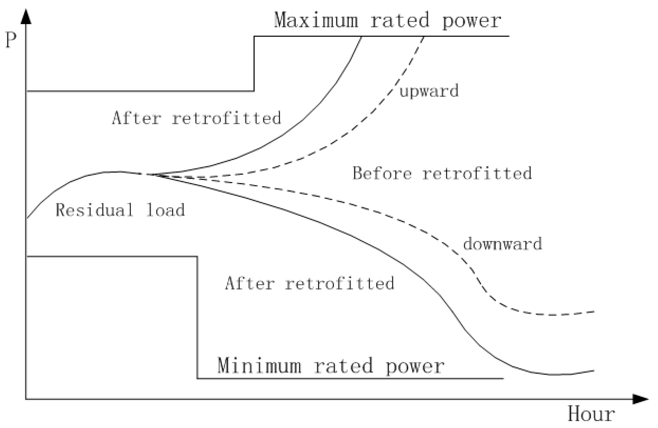
Figure 2.
Active power curves before and after ramp rate retrofitting.

Figure 3.
Highest flexible electricity in upward flexibility.

Figure 4.
Models for peak shaving depth retrofitting.
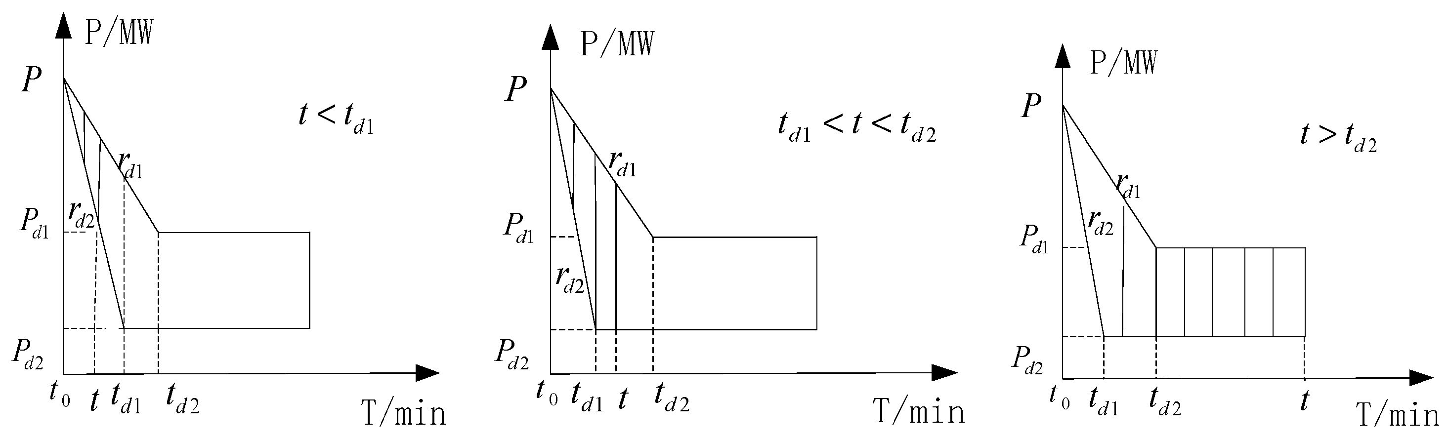
Figure 5.
Maximum flexibility with different depth and unified ramp rate.

Figure 6.
Maximum flexibility with the same depth and upward ladder ramp rate.

Figure 7.
Unit cost before and after retrofitting.

Figure 8.
Flexibility electricity from peak shaving depth retrofitting.


Table 1.
Five aspects of thermal power flexibility retrofitting.
| Retrofitted Target | Retrofitting Process | |
|---|---|---|
| 1 | The minimum output power can be reduced to 15–20% of the rated power. | Ensure: A. The stable combustion of the boiler B. The proper working of the environmental protection devices, such as desulfurizer. |
| 2 | The maximum ramp rate can be increased to 4–11% of the rated power. | Optimize the steam outlet valve of the steam turbine or raise the fuel calorific value of the boiler. |
| 3 | Different thermal state of units have different start–stop times. Gas power units: 0.1–1 h Coal power units: 2–7 h | Optimize dispatching management measures. Control the inlet temperature and speed of the boiler. Reduce the start–stop time of the boiler and the steam engine. |
| 4 | CHP units are firstly used for heating in the cold winter, and the by-product is electricity. Therefore the amount of electricity depends on heat amount. Make heat and electricity independent. | Add heat storage tanks for CHP units. When the power demand in the grid is low, the heat from the CHP units will be stored in heat storage tanks; and once power demand is high in the grid, the heat will be reused to generate electricity. |
| 5 | Replace fossil fuel combustion equipment with biomass fuels or peat. | Boiler reformation, improve the thermal efficiency and heat utilization rate of boilers. |
Note: this table was sorted by the authors.
Table 2.
Conventional generator parameter list [32].
Table 2.
Conventional generator parameter list [32].
| Node-Unit | |||
|---|---|---|---|
| 30-1 | 350 | 100 | 3 |
| 31-2 | 1145 | 600 | 7.4 |
| 32-3 | 750 | 250 | 4.2 |
| 33-4 | 732 | 250 | 4.2 |
| 34-5 | 608 | 250 | 3.5 |
| 35-6 | 750 | 250 | 4.2 |
| 36-7 | 660 | 250 | 3.5 |
| 37-8 | 640 | 250 | 3.3 |
| 38-9 | 930 | 250 | 5.3 |
| 39-10 | 1100 | 600 | 6 |
Table 3.
Ramp rate retrofitting scenarios (/).
| Node-unit | S1 | S2 | S3 | S4 | S5 |
|---|---|---|---|---|---|
| 30-1 | 4% | 5% | 6% | 7% | 8% |
| 14 | 17.5 | 21 | 24.5 | 28 | |
| 31-2 | 8% | 9% | 10% | 11% | 12% |
| 91.6 | 103.1 | 114.5 | 126 | 137.4 | |
| 32-3 | 6% | 7% | 8% | 9% | 10% |
| 45 | 52.5 | 60 | 67.5 | 70 | |
| 33-4 | 6% | 7% | 8% | 9% | 10% |
| 43.9 | 51.2 | 58.6 | 65.9 | 73.2 | |
| 34-5 | 5% | 6% | 7% | 8% | 9% |
| 30.4 | 36.5 | 42.6 | 48.6 | 54.7 | |
| 35-6 | 6% | 7% | 8% | 9% | 10% |
| 45.0 | 52.5 | 60.0 | 67.5 | 75.0 | |
| 36-7 | 5% | 6% | 7% | 8% | 9% |
| 33.0 | 39.6 | 46.2 | 52.8 | 59.4 | |
| 37-8 | 5% | 6% | 7% | 8% | 9% |
| 32.0 | 38.4 | 44.8 | 51.2 | 57.6 | |
| 38-9 | 7% | 8% | 9% | 10% | 11% |
| 65.1 | 74.4 | 83.7 | 93.0 | 102.3 | |
| 39-10 | 8% | 9% | 10% | 11% | 12% |
| 88 | 99 | 110 | 121 | 132 |
Table 4.
Upward flexibility elasticity coefficients of ramp rates.
| Unit | S2-S1 | S3-S2 | S4-S3 | S5-S4 | Optimized Range of Ramp Rate |
|---|---|---|---|---|---|
| 30-1 | 5.14 | 0.46 | 0.49 | 0.46 | 4–5% |
| 31-2 | 0.26 | 0.21 | 0.17 | 0.14 | 8–9% |
| 32-3 | 0.43 | 0.47 | 0.48 | 0.40 | 7–9% |
| 33-4 | 0.46 | 0.48 | 0.46 | 0.40 | 7–8% |
| 34-5 | 0.46 | 0.48 | 0.46 | 0.41 | 6–7% |
| 35-6 | 0.43 | 0.47 | 0.48 | 0.40 | 7–9% |
| 36-7 | 0.47 | 0.47 | 0.47 | 0.44 | 5–7% |
| 37-8 | 0.39 | 0.47 | 0.47 | 0.44 | 6–8% |
| 38-9 | 0.46 | 0.47 | 0.46 | 0.41 | 7–9% |
| 39-10 | 0.24 | 0.18 | 0.16 | 0.14 | 8–9% |
Table 5.
Operation parameters for peak shaving.
| Node-Unit | (Running Time for Reaching the Target Depth) | ||||||
|---|---|---|---|---|---|---|---|
| 30-1 | 3 | 18 * | 18 * | 19 * | 20 * | 20 * | |
| 31-2 | 7.4 | 8 | 9 | 9 | 10 | 11 | |
| 32-3 | 4.2 | 11 | 12 | 13 | 13 | 14 | |
| 33-4 | 4.2 | 11 | 12 | 13 | 13 | 14 | |
| 34-5 | 3.5 | 13 | 14 | 14 | 16 * | 17 * | |
| 35-6 | 4.2 | 11 | 12 | 13 | 13 | 14 | |
| 36-7 | 3.5 | 13 | 14 | 15 | 16 * | 21 * | |
| 37-8 | 3.3 | 13 | 14 | 15 | 16 * | 21 * | |
| 38-9 | 5.3 | 10 | 10 | 11 | 11 | 12 | |
| 39-10 | 6 | 8 | 9 | 9 | 10 | 11 | |
Note: All the starred values (*) represent that the unit cannot reach the retrofitted target within 15 min.
Table 6.
Peak shaving elasticity coefficient epeak.
| Node-Unit | A | B | C | D | Optimized Depth |
|---|---|---|---|---|---|
| 31-2 | 0.36 | 0.28 | 0.44 | 0.04 | C |
| 32-3 | 0.36 | 0.18 | 0.53 | 0.06 | C |
| 33-4 | 0.36 | 0.16 | 0.55 | 0.06 | C |
| 35-6 | 0.36 | 0.18 | 0.53 | 0.06 | C |
| 38-9 | 0.36 | 0.28 | 0.43 | 0.05 | C |
| 39-10 | 0.36 | 0.21 | 0.51 | 0.04 | C |
Notes: A represents the range of 20–25%Pn; B represents the range of 25–30%Pn; C represents the range of 20–25%Pn; D represents the range of 15–20%Pn.
Table 7.
Four scenarios for downward ramp rate set as upward ladders.
| Node-Unit | Sd1 | Sd2 | Sd3 | Sd4 |
|---|---|---|---|---|
| 30-1 | ||||
| 31-2 | ||||
| 32-3 | ||||
| 33-4 | ||||
| 34-5 | ||||
| 35-6 | ||||
| 36-7 | ||||
| 37-8 | ||||
| 38-9 | ||||
| 39-10 |
Table 8.
Downward ramp rate and running time .
| Unit | under Different Reaching the Target of | ||||
|---|---|---|---|---|---|
| Sd1 | Sd2 | Sd3 | Sd4 | ||
| 30-1 | 14.0 | 17.5 | 21.0 | 24.5 | |
| 20.0 * | 16.0* | 13.3 | 11.4 | ||
| 31-2 | 91.6 | 103.1 | 114.5 | 126.0 | |
| 10.0 | 8.9 | 8.0 | 7.3 | ||
| 32-3 | 45.0 | 52.5 | 60.0 | 67.5 | |
| 13.3 | 11.4 | 10.0 | 8.9 | ||
| 33-4 | 43.9 | 51.2 | 58.6 | 65.9 | |
| 13.3 | 11.4 | 10.0 | 8.9 | ||
| 34-5 | 30.4 | 36.5 | 42.6 | 48.6 | |
| 16.0 * | 13.3 | 11.4 | 10.0 | ||
| 35-6 | 45.0 | 52.5 | 60.0 | 67.5 | |
| 13.3 | 11.4 | 10.0 | 8.9 | ||
| 36-7 | 33.0 | 39.6 | 46.2 | 52.8 | |
| 16.0 * | 13.3 | 11.4 | 10.0 | ||
| 37-8 | 32.0 | 38.4 | 44.8 | 51.2 | |
| 16.0 * | 13.3 | 11.4 | 10.0 | ||
| 38-9 | 65.1 | 74.4 | 83.7 | 93.0 | |
| 11.4 | 10.0 | 8.9 | 8.0 | ||
| 39-10 | 88.0 | 99.0 | 110.0 | 121.0 | |
| 10.0 | 8.9 | 8.0 | 7.3 | ||
Note: All the starred values (*) represent that the unit cannot reach the retrofitted target within 15 min.
Table 9.
Elasticity coefficients and the best downward ramp rates.
| Node-Unit | Sd2-Sd1 | Sd3-Sd2 | Sd4-Sd3 | Optimized Downward Ramp Rate |
|---|---|---|---|---|
| 30-1 | 1.89 | 21.03 | 0.11 | 5–6% |
| 31-2 | 0.07 | 0.06 | 0.05 | 8–9% |
| 32-3 | 0.12 | 0.09 | 0.08 | 6–7% |
| 33-4 | 0.12 | 0.11 | 0.07 | 6–7% |
| 34-5 | 20.61 | 0.13 | 0.08 | 5–6% |
| 35-6 | 0.12 | 0.09 | 0.08 | 7–8% |
| 36-7 | 20.53 | 0.14 | 0.09 | 5–6% |
| 37-8 | 20.52 | 0.13 | 0.09 | 5–6% |
| 38-9 | 0.10 | 0.08 | 0.06 | 7–8% |
| 39-10 | 0.07 | 0.06 | 0.05 | 8–9% |
Table 10.
Peak shaving depth and retrofitting costs Cf(H).
| Depth () | 0.55 | 0.60 | 0.65 | 0.70 | 0.75 | 0.80 | 0.85 |
|---|---|---|---|---|---|---|---|
| Per Cost ( yuan/MW) | 50 | 75 | 100 | 125 | 150 | 175 | 200 |
| ( yuan) | 1.5 | 4.5 | 9.0 | 15.0 | 22.5 | 31.5 | 42.0 |
Note: Exchange rate is 1 $ = 6.88 RMB in 2017.
Table 11.
Peak shaving depth, heat rate and unit cost.
| Before Retrofitting | After Retrofitting | ||||||
|---|---|---|---|---|---|---|---|
| P/MW | Depth | kg/MWh | yuan/MWh | P/MW | Depth | kg/MWh | yuan/MWh |
| 600 | 0 | 299.6 | 179.8 | 600 | 0 | 299.6 | 179.8 |
| 550 | 0.08 | 319.7 | 191.4 | 550 | 0.08 | 320.7 | 192.4 |
| 500 | 0.16 | 339.4 | 203.6 | 500 | 0.16 | 340.8 | 204.5 |
| 450 | 0.25 | 359.8 | 215.9 | 450 | 0.25 | 360.9 | 216.5 |
| 400 | 0.33 | 377.6 | 226.6 | 400 | 0.33 | 380.0 | 228.0 |
| 350 | 0.42 | 389.0 | 233.4 | 350 | 0.42 | 395.1 | 237.1 |
| 300 | 0.50 | 399.3 | 239.6 | 300 | 0.50 | 414.2 | 248.5 |
| - | - | - | - | 250 | 0.58 | 433.3 | 260.0 |
| - | - | - | - | 200 | 0.67 | 452.4 | 271.4 |
| - | - | - | - | 150 | 0.75 | 463.0 | 277.8 |
| - | - | - | - | 90 | 0.85 | 472.4 | 283.4 |
Table 12.
Flexible electricity compensation scenarios (unit: yuan/MWh).
| Depth | 0–0.50 | 0.50–0.60 | 0.60–0.70 | 0.70–0.85 |
| 0 | 0.0004 | 0.0006 | 0.0008 | |
| Depth | 0–0.40 | 0.40–0.85 | ||
| 0.0004 | 0.001 | 0.001 | 0.001 |
Table 13.
for and the total annual running hours in the basic scenario.
| (0.50, 0.60] | (0.60, 0.70] | (0.70, 0.85] | |
| 0.0004 | 0.0006 | 0.0008 | |
| (55, 305] | (203, 355] | (277, 402] | |
| Total annual peak shaving running hours | |||
| (14, 76] | (51, 89] | (69, 101] | |
| (28, 152] | (102, 198] | (138, 201] | |
| (42, 228] | (153, 267] | (207, 303] | |
| (55, 305] | (203, 355] | (277, 402] | |
Table 14.
for and the total annual running hours in the policy scenario.
| (0.50, 0.60] | (0.60, 0.70] | (0.70, 0.85] | |
| 0.001 | |||
| (22, 322] | |||
| Total annual peak shaving running hours | |||
| T = 0.25 h | (4, 81] | ||
| T = 0.50 h | (8, 162] | ||
| T = 0.75 h | (12, 243] | ||
| T = 1.0 h | (22, 322] | ||
Table 15.
Peak shaving hours of Jilin Province.
| Items | Jilin Province | |
|---|---|---|
| Curtailed wind power (GWh) | 2900 | |
| Total coal power flexibility retrofitting capacity(GW) | 13.30 | |
| Peak shaving operation hours (h) | the depth from 0.50 to 0.60 | 2180 |
| the depth from 0.5 to 0.70 | 1090 | |
| the depth from 0.50 to 0.85 | 727 | |
Table 16.
Characteristic roots of two scenarios.
| (0.50, 0.60] | (0.60, 0.70] | (0.70, 0.85] | |||
| 0.0004 | 0.0006 | 0.0008 | |||
| 0.5182 | 0.5382 | 0.5582 | |||
| Decision and compensation standard | Yes, enough for | No, not enough | No, not enough | ||
| 0.5982 | 0.6582 | 0.7182 | |||
| Decision and compensation standard | Yes, enough for | Yes, enough for | Yes, enough for | ||
| 0.6782 | 0.7782 | 0.8782 | |||
| Decision and compensation standard | Yes, high | Yes, high | Yes, high | ||
| 0.001 | |||||
| , Decision and compensation standard | 0.5782, Yes, enough for | ||||
| 0.7782, Yes, enough for | |||||
| 0.9782, Yes, high compensation standard | |||||
Table 17.
All the conclusions and the determinants.
| Conclusions | Determinants | |
|---|---|---|
| 1 | Upward ramp rate | Upward elastic coefficient |
| Downward ramp rate | Downward elastic coefficient | |
| Peak shaving depth | Peak shaving elastic coefficient | |
| 2 | Economic decision-making | Depth, compensation standard, times |
| Compensation standard | Depth, times | |
© 2018 by the authors. Licensee MDPI, Basel, Switzerland. This article is an open access article distributed under the terms and conditions of the Creative Commons Attribution (CC BY) license (http://creativecommons.org/licenses/by/4.0/).
Share and Cite
MDPI and ACS Style
Na, C.; Yuan, J.; Zhu, Y.; Xue, L. Economic Decision-Making for Coal Power Flexibility Retrofitting and Compensation in China. Sustainability 2018, 10, 348. https://doi.org/10.3390/su10020348
AMA Style
Na C, Yuan J, Zhu Y, Xue L. Economic Decision-Making for Coal Power Flexibility Retrofitting and Compensation in China. Sustainability. 2018; 10(2):348. https://doi.org/10.3390/su10020348
Chicago/Turabian StyleNa, Chunning, Jiahai Yuan, Yuhong Zhu, and Li Xue. 2018. "Economic Decision-Making for Coal Power Flexibility Retrofitting and Compensation in China" Sustainability 10, no. 2: 348. https://doi.org/10.3390/su10020348
Note that from the first issue of 2016, this journal uses article numbers instead of page numbers. See further details here.