Supplier Selection Study under the Respective of Low-Carbon Supply Chain: A Hybrid Evaluation Model Based on FA-DEA-AHP

Abstract

With the development of global environment and social economy, it is an indispensable choice for enterprises to achieve sustainable growth through developing low-carbon economy and constructing low-carbon supply chain. Supplier is the source of chain, thus selecting excellent low-carbon supplier is the foundation of establishing efficient low-carbon supply chain. This paper presents a novel hybrid model for supplier selection integrated factor analysis (FA), data envelopment analysis (DEA), with analytic hierarchy process (AHP), namely FA-DEA-AHP. First, an evaluation index system is built, incorporating product level, qualification, cooperation ability, and environmental competitiveness. FA is utilized to extract common factors from the 18 pre-selected indicators. Then, DEA is applied to establish the pairwise comparison matrix and AHP is employed to rank these low-carbon suppliers comprehensively and calculate the validity of the decision-making units. Finally, an experiment study with seven cement suppliers in a large industrial enterprise is carried out in this paper. The results reveal that the proposed technique can not only select effective suppliers, but also realize a comprehensive ranking. This research has enriched the methodology of low-carbon supplier evaluation and selection, as well as owns theoretical value in exploring the coordinated development of low-carbon supply chain to some extent.

1. Introduction

In recent years, with the burgeoning development of economic society, increasing energy consumption and serious environmental pollution have ensued, in particular, the dramatic growth in carbon dioxide has led to global warming and the rise of sea level [1]. Governments are dedicated to “Low-Carbon Revolution and Circular Economy” around the world through promulgation of policy and encouragement to enterprises on taking both economic and environmental benefits into account [2,3]. Accordingly, enterprises, especially production-oriented ones, are bound to change their traditional operation modes to reduce carbon emissions as well as costs [4]. Centobelli et al. [5,6] conducts a structured review on the topic of energy efficiency, environmental sustainability, and taxonomy of green initiatives in the supply chain management context. Simultaneously, improvement of the public’s awareness on low-carbon environmental protection makes it remarkably intense for the demand of related products [7]. Thus, it is imperative for suppliers to fulfill the customer’s low-carbon requirements during the supply chain management.

A research implemented by TRUCOST shows only 19% greenhouse gases in the supply chain directly come from business operation, while the indirect sources contributes the other 81% [8], such as Tier One Suppliers, power suppliers, and other members. Indeed, the selection of suitable suppliers is an approach to react to carbon emission reduction from the fountainhead, which can lower both the environmental governance and risk commitment burden. Thus, increased attention has been paid to the choice of low-carbon suppliers in the scientific researches.

Throughout recent studies, supplier selection can be achieved by two steps: design an evaluation index system and propose an applicable model [9,10,11]. In the case of index system associated with supplier selection, the researches accomplished by Dickson and Weber have laid a momentous basis for the subsequent studies at home and abroad. Dickson [12] sorted out 23 indicators for supplier evaluation by a questionnaire and made a comparison on their importance, which pointed out that quality, delivery period, and historical performance were top three vital indexes. Weber et al. [13,14] summarized 23 evaluation principles via 74 literature for 33 years and proved price, delivery period, quality, equipment and capability, geographical location, and technique were of great significance by means of statistical analysis. Hereafter, green supplier evaluation and selection has started with the choice of environment as an important factor. Hanfield et al. [15] adopted Delphi method to extract ten most momentous factors of supplier evaluation in green procurement including environmental records released to the public, Tier Two supplier environmental assessment, hazardous waste disposal, toxic waste pollution management, ISO14000 certification, reverse logistics projects, environmentally friendly product packaging, utilization of ozone-depleting substances, and administration of hazardous gas emissions. A novel evaluation index, namely hazardous materials, was proposed by Hsu and Hu [16], which consists of green procurement, green material code and record, green design capability, harmful substance inventory and management, compliance as well as environmental administration system. When considering green image, product recycling, green design, green supply chain management, pollution control cost, and environmental performance, Yeh and Chuang [17] introduced multi-objective model to make a decision on green partner selection that focused on four goals, that is, cost, time, quality, and green assessment score. Carbon emission and carbon management involved in the study of green supplier option come into being along with the emergence of “Low-Carbon Revolution”. Hsu et al. [18] pointed out that carbon information management system and related training were conducive to competitive supplier selection. The index system put forward by Shaw et al. [19] incorporated cost, quality rejection rate, delayed delivery rate, greenhouse gas emission, and demand.

The research in supplier selection evaluation measures can be divided into two categories: One is qualitative analysis, such as intuitive judgement, negotiation, and bidding [20,21]. Though these methods are relatively simple and easy to implement, most of them as based on empirical or certain deterministic criteria attached to strong subjectivity. The other is quantitative approach that can be further classified into three parts. (1) Multi-attribute decision-making method, such as analytic hierarchy process (AHP), analytic network process, multi attribute utility theory, the technique for order preference by similarity to the ideal solution. Felix et al. [22] aimed at taking both quantitative and qualitative influential factors into account and developed fuzzy based AHP to choose global supplier in the current commercial scenario. Kang et al. [23] utilized IC packaging company selection in Taiwan as an experiment to make a selection among suppliers by fuzzy analytic network. In order to effectively deal with decision maker’s fuzzy goals in supplier option, a method integrated with multi attribute utility theory was presented in reference [24]. Sahin and Yigider [25] came up with an improved TOPSIS approach to handle complicated factors. (2) Programming method mainly encompassing linear programming, goal programming, and mixed integer programming. Nazari-Shirkouhi et al. [26] employed a multi-objective linear programming model to balance multi-price and multi-product in supplier evaluation. An approach for multi-choice and multi-segment goal programming and a mixed integer programming method were applied to cope with the supplier selection in reference [27] and [28], respectively. (3) Artificial intelligence, containing neural network, genetic algorithm, support vector machine (SVM), and so on. Kuo et al. [29] designed a neural network based model to analyze quantitative and qualitative indicators in supplier decision. An integrated genetic algorithm was adopted by Sadeghieh [30], while reference [31] combined SVM with hierarchical system of feature to address the problem of supplier selection.

In general, based on the aforementioned studies, it can be found that the issue of supplier selection has attracted wide attention for decades. The corresponding evaluation index system and models tend to be more and more scientific. Nevertheless, the development of information and low-carbon economy bring about changes in assessing suppliers, namely enterprise compatibility, deliver ability, environmental protection capability should be taken into consideration. Accordingly, the evaluation and selection technique should also be better adapted to the variety of index system so as to make the results more accurate and intuitive.

Therefore, a new index system is built in this paper that covers product quality, enterprise qualification, cooperation ability, and environmental competitiveness. Moreover, a hybrid model that integrates factor analysis (FA) and data envelopment analysis (DEA) with AHP is put forward to make a research on low-carbon supplier option. FA is exploited to reduce the dimension of pre-selected factors through extracting several comprehensive indicators to reflect the characteristics of original data [32]. In view of multi-input and multi-output elements, as well as non-linearity in low-carbon supplier selection, in coincidence with the multi-objective decision-making method DEA, the paper applied this technique to cope with the problem. However, it is noted that the consequences of DEA can merely be parted as effectiveness, weak effectiveness and ineffectiveness, which still can’t identify the best one. Thus, AHP is introduced to compensate the shortcomings by establishment of a hierarchical structure and quantization of the influence of each factor on the final results with weight. The rest of the paper is organized as follows: Section 2 builds the evaluation index system of low-carbon suppliers. Section 3 shows the framework of the proposed evaluation technique FA-DEA-AHP, while Section 4 illustrates the case study with seven low-carbon cement suppliers in a Chinese industrial enterprise. Section 5 makes a discussion on the results derived from the model. In the end, Section 6 concludes the paper.

2. The Construction of Low-Carbon Supplier Evaluation and Selection Index System

There is still not a unified standard for establishment of index system for supplier selection in terms of preceding studies in the Introduction. Moreover, different levels of cooperation between suppliers and enterprises and types of business provided by suppliers also lead to great difference in evaluation indicators.

The construction of supplier evaluation and selection index system in low-carbon supply chain aims at revealing the characteristics of supplier assessment under the fire-new environment and competition conditions. Based on previous studies at home and abroad [13,14,18,19], the evaluation index system of supplier selection proposed in this paper is built from four aspects: product level, qualification, cooperation ability, and environmental competitiveness, as shown in

Table 1. Evaluation index system of low-carbon supplier selection.

Evaluation Objective	Level Indicators	Secondary Indicators	Indicator Type
Evaluation index system of low-carbon supplier selection	Product level	Product qualification rate	quantitative
		Quality management system	qualitative
		Quality improvement plan	qualitative
		Relative price level	quantitative
	Qualification	The rate of return on total assets	quantitative
		Quick ratio	quantitative
		Profit growth rate	quantitative
		Per employee training time,	quantitative
		Equipment	qualitative
		Input rate of research funding	quantitative
	Cooperation ability	On-time delivery rate	quantitative
		Order completion rate,	quantitative
		Enterprise reputation	qualitative
		Information level	qualitative
		Strategic objective Compatibility	qualitative
	Environmental competitiveness	Carbon dioxide emission	quantitative
		“Three wastes” recycling rate	quantitative
		Environmental amelioration cost	quantitative

.

The definitions of the above indexes are given here so as to make them understood clearly.

(1).

Production qualification rate is equal to the percentage of qualified products in the total procurement within a period of time.

(2).

Quality management system is imperative for quality assurance. Total quality management (TQM) and ISO standard series are employed here to carry out this appraisal.

(3).

Quality improvement plan refers to assessment of supplier’s future quality administration, particularly the strategic partners.

(4).

Relative price level can be obtained through the comparison of supplier’s product price with that of the industry on the average.

(5).

The rate of return on total assets is equal to the whole amount of remuneration acquired by the enterprise divided by average total assets, which reflects the profitability of all the assets.

(6).

Quick ratio is equal to quick assets divided by current liabilities, which shows the ability of suppliers in immediate wealth realization and repayment of current liabilities.

(7).

Profit growth rate is equal to the difference of profits between the previous period and the current one divided by the profit in the prior period. This index represents supplier’s development ability in finance.

(8).

Per employee training time is necessary to enhance staffs’ energy saving and environmental protection awareness as well as master new technologies, besides the encouragement of policy-making and technological innovation and application. The index is equal to training days divided by the number of trained employees.

(9).

Equipment directly affects the formulation of product techniques and further has an effect on production capacity, which reflects whether advanced technology is adopted.

(10).

Input rate of research funding equals research funds divided by sales revenue over a period of time as a symbol of R&D capability.

(11).

On-time delivery rate examines suppliers’ delivery capacity, represented by the total number of delivery on time divided by whole times of delivery.

(12).

Order completion rate is expressed as completed orders divided by total ones, which reflects suppliers’ satisfaction to customers’ purchasing needs.

(13).

Enterprise reputation can be acquired through the credit rating given by banks and customers.

(14).

Information level stands for the ability of suppliers and enterprise to exchange and share information, as well as represents the technical basis of suppliers’ quick response to urgent orders.

(15).

Strategic objective compatibility reflects whether the supply chain is coordinated. This paper will particularly focuses on the low-carbon strategic target in supplier selection.

(16).

Carbon dioxide emission is calculated by the method of carbon emission factor, which indicates the amount of greenhouse gas emitting during production.

(17).

“Three-wastes” recycling rate refers to the recycling proportion of waste gas, waste water and waste residues generated during production and operation.

(18).

Environmental amelioration cost equals the expenses that the enterprise invests on environmental improvement and pollution control in a period of time.

3. Low-Carbon Supplier Selection Approach Based on FA-DEA-AHP

3.1. FA

FA refers to a species of statistical method that extracts information and simplifies data by dimension reduction. The main steps are shown as follows [32]:

(1) Test whether FA can be implemented on the variables. FA picks up common factors from a group of relevant variables. This technique will be invalid if variables are independent of each other or the overlap of information is small. Thus, it is imperative to carry out correlation analysis, mainly the Kaiser-Meyer-Olkin (KMO) test and Barylett test of sphericity.

(2) Identify common factors and determine the number by means of maximum likelihood estimate, least square method or principal component analysis (PCA), and so on. PCA, selected in this paper, is a technique that transforms normalized variables into irrelevant ones by coordinate alternation. Through calculating the eigenvalue ${\lambda }_i$ and corresponding standard orthogonal eigenvector $l_i$, the factor loading matrix $A$ can be derived from Equations (1) and (2).

$$a_{ij}=\sqrt{{\lambda }_i}{l}_{ij}$$

(1)

$$A=\left[\begin{array}{cccc}{a}_{11}& a_{12}& \cdots & a_{1m}\\ a_{21}& a_{22}& \cdots & a_{2m}\\ ⋮& ⋮& \ddots & ⋮\\ a_{p1}& a_{p2}& \cdots & a_{pm}\end{array}\right]=\left[\begin{array}{cccc}{l}_{11}\sqrt{{\lambda }_1}& l_{12}\sqrt{{\lambda }_2}& \cdots & l_{1m}\sqrt{{\lambda }_m}\\ l_{21}\sqrt{{\lambda }_1}& l_{22}\sqrt{{\lambda }_2}& \cdots & l_{2m}\sqrt{{\lambda }_m}\\ ⋮& ⋮& \ddots & ⋮\\ l_{p1}\sqrt{{\lambda }_1}& l_{p2}\sqrt{{\lambda }_2}& \cdots & l_{pm}\sqrt{{\lambda }_m}\end{array}\right]$$

(2)

Variance contribution rate, namely square sum of elements of the $j$-th column in matrix $A$, describes the total information extracted by common factors $F_j$. The higher the variance contribution rate is, the more significant the common factor is. Generally, in order to enhance the interpretability of the factors, loading matrix $A$ needs to be rotated so that elements in each row are divided into 0 and 1.

For the determination of the number of common factors, there ordinarily exists two approaches, choosing the factors of which eigenvalues are more than 1 or accumulative explained variation that accounts for the proportion of information in original indexes is over 0.85.

(3) Name the common factors. The nomenclature is customarily based on the rotated factor loading matrix. The common factor with large load illustrates the pre-selected variables have a strong correlation, thus it can be name after the mutual meaning of the bracketed variables.

(4) Calculate factor scores. The regression technique can be expressed as Equation (3).

$$F_j=b_{i0}+b_{j1}{x}_1+b_{j2}{x}_2+\cdots +b_{jp}{x}_p\left(j=1,2,\cdots ,m\right)$$

(3)

where $\left(b_{j1},b_{j2},\cdots ,b_{jp}\right)$ is the factor score vector, ${\left(x_1,x_2,\cdots ,x_p\right)}^T$ equals variable vector.

In this way, the samples can be distinctly compared according to the scores of common factors in all aspects.

3.2. DEA

DEA is an approach based on the concept of relative efficiency and employs convex analysis and linear programming as techniques. The main steps are explained as follows [33]:

Suppose that there are $n$ low-carbon suppliers, called $n$ decision making units (DMUs). Each DMU owns $m$ inputs and $p$ outputs expressed by different evaluation indicators.

The linear programming model of DEA can be mathematically presented as Equation (4).

$$\left(P\right)\{\begin{array}{l}\max V_p={\mu }^T{y}_0\\ \mathrm{s}.\mathrm{t}.{\omega }^T{x}_j-{\mu }^T{y}_j\ge 0,1\le j\le n\\ {\omega }^T{x}_0=1\\ \omega \ge 0,\mu \ge 0\end{array}$$

(4)

where $x_{ij}$ is input $i$ of DMU_j, $x_{ij}>0$, $y_{rj}$ is output $r$ of DMU_j, $y_{rj}\ge 0$; $v_i$ represents the weight assigned to input $i$, $v_i\ge 0$, $u_r$ equals the weight assigned to output $r$, $u_r\ge 0$; $v={\left(v_1,v_2,\cdots ,v_m\right)}^T$, $u={\left(u_1,u_2,\cdots ,u_p\right)}^T$, $t=1/v^T{x}_0$, $\omega =tv$, $\mu =tu$.

To make DEA more practical, non-Archimedean infinitesimal $\epsilon$ is introduced, as shown in Equation (5).

$$\left(P_{\epsilon }\right)\{\begin{array}{l}\max {\mu }^T{y}_0=V_{P_{\epsilon }}\\ \mathrm{s}.\mathrm{t}.{\omega }^T{x}_j-{\mu }^T{y}_j\ge 0,1\le j\le n\\ {\omega }^T{x}_0=1\\ {\omega }^T\ge \epsilon {\widehat{e}}^T,{\mu }^T\ge \epsilon e^T\end{array}$$

(5)

where ${\widehat{e}}^T$ and $e^T$ are the $m$ and $p$ dimension unit vectors, respectively.

The dual programming of $\left(P_{\epsilon }\right)$ is written as Equation (6):

$$\left(D_{\epsilon }\right)\{\begin{array}{l}\min \left[\theta -\epsilon \left({\widehat{e}}^T{s}^{-}+e^T{s}^{+}\right)\right]=V_{D_{\epsilon }}\\ \mathrm{s}.\mathrm{t}.{\displaystyle \sum _{j=1}^n{x}_j{\lambda }_j+s^{-}={\theta }_{x_0}}\\ {\displaystyle \sum _{j=1}^n{y}_j{\lambda }_j-s^{+}=y_0}\\ {\lambda }_j\ge 0,1\le j\le n,s^{-}\ge 0,s^{+}\ge 0\end{array}$$

(6)

where $s^{-}={\left(s_1^{-},s_2^{-},\cdots ,s_m^{-}\right)}^T$ and $s^{+}={\left(s_1^{+},s_2^{+},\cdots ,s_m^{+}\right)}^T$ are slack variables.

3.3. AHP

AHP is a decision-making method combining qualitative and quantitative analysis based on the multiple hierarchy structure incorporating objectives, criteria, and projects. The priorities of elements in every hierarchy can be obtained as follows [34]:

(1) Establish the pairwise comparison matrix. Suppose there are $n$ elements, $b_{ij}$ stands for the relative importance of element $i$ in contrast with element $j$.

$$B={\left(b_{ij}\right)}_{n\times n}=\left[\begin{array}{cccc}{b}_{11}& b_{12}& \cdots & b_{1n}\\ b_{12}& b_{22}& \cdots & b_{2n}\\ ⋮& ⋮& \ddots & ⋮\\ b_{n1}& b_{n2}& \cdots & b_{nn}\end{array}\right]$$

(7)

where $B$ is the pairwise comparison matrix and $b_{ij}=1/b_{ji}$.

(2) Derive the priorities. Calculate the largest eigenvalue ${\lambda }_{\max }$ and the corresponding eigenvector $W$ of matrix $B$, that is, $BW={\lambda }_{\max }W$ and $\left(w_1,w_2,\cdots ,w_n\right)$ equals the importance ranking of the elements.

(3) Test the consistency of the judgements. If the judgement is completely consistent, ${\lambda }_{\max }=n$, otherwise ${\lambda }_{\max }>n$. Thus, ${\lambda }_{\max }-n$ can be used as a measure of the deviation from the coherence.

$$CI=\frac{{\lambda }_{\max }-n}{n-1}$$

(8)

$$CR=CI/RI$$

(9)

where $CI$ and $RI$ are the consistency indicator and random index, respectively. $CR$ refers to the random consistency ratio. The comparison matrix is coincident if $CR\le 0.01$, otherwise the comparison matrix needs to be modified until the test is satisfied. The values of $RI$ obtained from random 500 samples are listed in

Table 2. The values of $RI$ obtained from random 500 samples.

n	3	4	5	6	7	8	9	10
RI	0.52	0.89	1.12	1.26	1.36	1.41	1.46	1.49

[34].

3.4. Low-Carbon Supplier Selection on the Basis of FA-DEA-AHP

FA-DEA-AHP proposed in this paper can be constructed according to the following steps:

(1) Division of input and output indicators. According to the index system recorded in Table 1, the indexes can be decomposed into two parts: input indexes required to be consumed and output indexes attached to effects in management, as shown in

Table 3. Inputs and Outputs in low-carbon supplier selection.

Inputs	quality management system, quality improvement plan, relative price level, per employee training time, equipment, environmental amelioration cost, input rate of research funding
Outputs	product qualification rate, the rate of return on total assets, quick ratio, profit growth rate, on-time delivery rate, order completion rate, enterprise reputation, information level, strategic objective compatibility, carbon dioxide emission, “three wastes” recycling rate

.

(2) Refinement and simplification of the pre-selected indexes by FA.

(3) Establishment of comparison matrixes by DEA. Randomly choose two low-carbon suppliers $M$ as well as $N$, then calculate the relative efficiency values ${\theta }_{MN}$ and ${\theta }_{NM}$ according to Equation (6).

$$\{\begin{array}{l}\min \left[{\theta }_{MN}-\epsilon \left({\widehat{e}}^T{s}^{-}+e^T{s}^{+}\right)\right]=V_{D_{\epsilon }}\\ \mathrm{s}.\mathrm{t}.{\displaystyle \sum _{j=1}^n{x}_j{\lambda }_j+s^{-}={\theta }_{MN}}\\ {\displaystyle \sum _{j=1}^n{y}_j{\lambda }_j-s^{+}=y_M}\\ {\lambda }_j\ge 0,1\le j\le n,s^{-}\ge 0,s^{+}\ge 0\end{array}$$

(10)

$$\{\begin{array}{l}\min \left[{\theta }_{NM}-\epsilon \left({\widehat{e}}^T{s}^{-}+e^T{s}^{+}\right)\right]=V_{D_{\epsilon }}\\ \mathrm{s}.\mathrm{t}.{\displaystyle \sum _{j=1}^n{x}_j{\lambda }_j+s^{-}={\theta }_{NM}}\\ {\displaystyle \sum _{j=1}^n{y}_j{\lambda }_j-s^{+}=y_N}\\ {\lambda }_j\ge 0,1\le j\le n,s^{-}\ge 0,s^{+}\ge 0\end{array}$$

(11)

The relative efficiency of low-carbon suppliers $M$ and $N$, namely $b_{MN}$ or $b_{NM}$ can be derived from Equations (12) and (13).

$$b_{MN}={\theta }_{MN}/{\theta }_{NM}$$

(12)

$$b_{NM}={\theta }_{NM}/{\theta }_{MN}=1/b_{NM}$$

(13)

$b_{MN}<1$ means supplier $M$ is superior to supplier $N$; $b_{MN}=1$ represents supplier $M$ is equivalent to supplier $N$; $b_{MN}>1$ indicates supplier $M$ is inferior to supplier $N$. Thus, the comparison matrix can be achieved on the foundation of Equation (7).

(4) Sequence and selection of low-carbon suppliers using AHP. The validity of DEA for each supplier can also be judged.

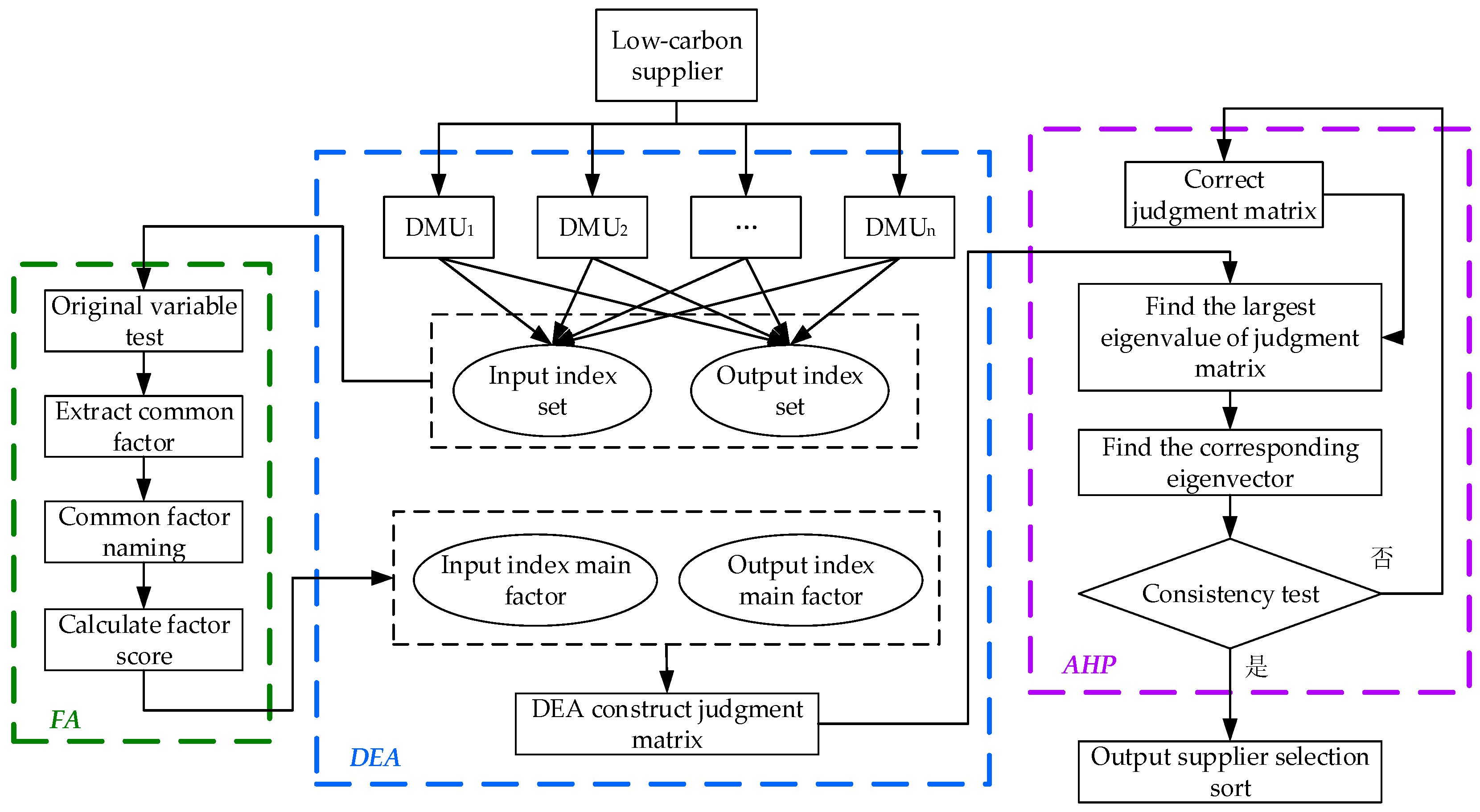
Low-carbon supplier selection technique incorporating FA, DEA, and AHP is built, as illustrated in Figure 1.

4. Case Study

A large steel enterprise in China, integrating mining, smelting, processing, and building construction as a whole, is chosen as an example in this paper. This company positively responds to low-carbon policy, but pays no special attention to the choice of low-carbon supplier. In order to demonstrate the efficiency of the proposed model, seven available cement suppliers are selected as samples. Through the historical information of the suppliers, the qualitative indicators are scored by relevant leaders (the criteria are shown in the Appendix A).

FA is firstly exploited to extract common factors from the seven inputs and eleven outputs listed in Table 1. The results of KMO and Bartlett’s sphericity test can be attained from the following

Table 4. Kaiser-Meyer-Olkin (KMO) test and Bartlett’s sphericity test results of various factors.

KMO test		0.814
Bartlett’s sphericity test	Chi-square test	154.627
	Degree of freedom	36
	Significance indicator	0.000

. The statistic value of KMO is generally between 0 and 1, the closer to 1 KMO is, the more appropriate for FA the variable is. The value of KMO in Table 4 equals 0.814, which proves that FA can be applied. Additionally, the significant probability of Bartlett’s sphericity test is 0.000, denying the correlation matrix is a unit one.

The common factors whose eigenvalues are over 1 are obtained by PCA in accordance with Equations (1) and (2). As we can see, the accumulative contribution rate of the four extracted common factors for outputs in

Table 5. The total explained variance of output indicators.

Composition	Initial Eigenvalue			The Sum of the Extracted Loads Squared			Rotational Sum of Squares
	Total	Variance Contribution Rate/%	Cumulative Variance Contribution Rate/%	Total	Variance Contribution Rate/%	Cumulative Variance Contribution Rate/%	Total	Variance Contribution Rate/%	Cumulative Variance Contribution Rate/%
1	4.787	45.420	45.420	4.787	45.420	45.420	3.767	35.385	35.385
2	2.414	21.926	67.346	2.414	21.926	67.346	2.275	23.627	59.012
3	1.878	19.070	86.416	1.878	19.070	86.416	2.267	20.364	79.376
4	0.831	8.633	95.049	0.831	8.633	95.049	1.607	15.673	95.049
5	0.427	3.961	99.010
6	0.110	0.990	100.000
7	2.506 × 10−16	2.269 × 10−15	100.000
8	5.056 × 10−16	1.768 × 10−15	100.000
9	−6.057 × 10−16	−5.406 × 10−16	100.000
10	−1.660 × 10−16	−1.509 × 10−15	100.000
11	−3.054 × 10−16	−2.675 × 10−15	100.000

can be 96.965%, which indicates a large majority of information in original variables is summarized.

Table 6. Factor loading matrix of output indicators.

Composition	1	2	3	4
Information level	0.942	0.164	−0.256	−0.160
Strategic objective compatibility	0.865	0.179	−0.301	−0.029
enterprise reputation	0.835	0.239	−0.390	0.054
“Three wastes” recycling rate	−0.043	0.683	0.368	0.358
carbon dioxide emission	0.032	0.858	−0.336	−0.270
The rate of return on total assets	−0.298	0.259	0.898	0.413
Quick ratio	0.283	−0.478	0.750	−0.441
Profit growth rate	0.409	−0.278	0.850	−0.172
On-time delivery rate	0.234	0.442	−0.168	0.774
Order completion rate	0.067	0.319	−0.427	0.894
Product qualification rate	0.214	−0.356	0.419	0.712

and

Table 7. Rotated factor loading matrix.

Composition	1	2	3	4
Information level	0.959	0.013	−0.003	0.002
Strategic objective compatibility	0.913	0.006	−0.243	−0.150
enterprise reputation	0.885	0.017	−0.295	0.058
“Three wastes” recycling rate	−0.062	0.721	−0.401	0.229
carbon dioxide emission	0.023	0.932	−0.235	−0.149
The rate of return on total assets	0.300	0.278	0.839	0.137
Quick ratio	−0.458	−0.122	0.733	−0.279
Profit growth rate	0.201	0.164	0.967	−0.007
On−time delivery rate	0.313	0.199	−0.077	0.793
Order completion rate	−0.275	0.242	0.123	0.906
Product qualification rate	0.246	−0.493	0.391	0.676

presents the factor loading matrix and the deformation rotated by Varimax, respectively.

As can be seen in Table 7, the first common factor has high load on information level (0.959), strategic objective compatibility (0.913), and enterprise reputation (0.885), nominated as credit cooperation factor. Similarly, the second factor is defined as low-carbon environmental factor, with high load on carbon dioxide emission (0.932) and “three wastes” recycling rate (0.721). The third common factor owing high load on the rate of return on total assets (0.939), quick ratio (0.733), and profit growth rate (0.967), as well as the fourth common factor with high load on product qualification rate (0.793), on-time delivery rate (0.906), and order completion rate (0.676) are respectively designated as economic level factor and supply capacity factor.

Table 8. Factor scores of output indicators.

Supplier	Credit Cooperation Factor	Low-Carbon Environmental Factor	Economic Level Factor	Supply Capacity Factor
1	−0.92493	−1.37460	−0.92339	−1.10503
2	1.13748	−0.90202	−0.82769	1.21883
3	1.31824	0.50494	0.25635	−1.40839
4	−0.05264	0.28902	1.03412	−0.38808
5	0.01768	1.45621	−1.12308	0.46748
6	−0.01851	−0.59661	1.46775	0.83478
7	−1.48441	0.61398	0.12503	0.37132

shows common factor scores derived from Equation (3).

Since there exists negative numbers in the original data, normalization is imperative as shown in

Table 9. Normalized factor scores of output indexes.

Supplier	Credit Cooperation Factor	Low-Carbon Environmental Factor	Economic Level Factor	Supply Capacity Factor
1	0.28	0.10	0.17	0.20
2	0.94	0.25	0.20	1.00
3	1.00	0.70	0.58	0.10
4	0.56	0.63	0.85	0.45
5	0.58	1.00	0.10	0.74
6	0.57	0.35	1.00	0.87
7	0.10	0.73	0.53	0.71

.

Analogously, FA is implemented on input indicators and two common factors are obtained for original seven input indexes whose accumulative contribution rate reaches 86.34%. There, into the quality management system, quality improvement plan, and relative price level present a high load on the first common factor, named as product level factor, while per employee training time, equipment, input rate of research funding, and environmental amelioration cost have a high load on the second common factor designated as business security factor. The final score of input indexes are listed in

Table 10. Normalized factor scores of output indexes.

Supplier	Product Level Factor	Business Security Factor
1	1.00	0.24
2	0.56	0.10
3	0.10	0.18
4	0.24	0.58
5	0.95	0.53
6	0.55	0.75
7	0.74	1.00

.

According to the DEA model, seven suppliers can be regarded as seven DMUs. Each factor has two input indicators and four output indicators for each DMU, as shown in

Table 11. Low carbon supplier input and output data.

DMU	DMU1	DMU2	DMU3	DMU4	DMU5	DMU6	DMU7
x1	1.00	0.56	0.10	0.24	0.95	0.55	0.74
x2	0.24	0.10	0.18	0.58	0.53	0.75	1.00
y1	0.28	0.94	1.00	0.56	0.58	0.57	0.10
y2	0.10	0.25	0.70	0.63	1.00	0.35	0.73
y3	0.17	0.20	0.58	0.85	0.10	1.00	0.53
y4	0.20	1.00	0.10	0.45	0.74	0.87	0.71

.

Calculate the pairwise relative efficiency of DMUs. Here, DMU₁ and DMU₂ are taken as an example, according to Equations (10) and (11).

$$\{\begin{array}{l}\min \left[\theta -\epsilon \left(s_1^{-}+s_2^{-}+s_1^{+}+s_2^{+}+s_3^{+}+s_4^{+}\right)\right]\\ 1.00{\lambda }_1+0.56{\lambda }_2+s_1^{-}=1.00\theta \\ 0.24{\lambda }_1+0.10{\lambda }_2+s_1^{-}=0.24\theta \\ 0.28{\lambda }_1+0.94{\lambda }_2-s_1^{+}=0.28\\ 0.10{\lambda }_1+0.25{\lambda }_2-s_2^{+}=0.10\\ 0.17{\lambda }_1+0.20{\lambda }_2-s_3^{+}=0.17\\ 0.20{\lambda }_1+1.00{\lambda }_2-s_4^{+}=0.20\end{array}$$

$${\theta }_{12}=0.3587$$

$$\{\begin{array}{l}\min \left[\theta -\epsilon \left(s_1^{-}+s_2^{-}+s_1^{+}+s_2^{+}+s_3^{+}+s_4^{+}\right)\right]\\ 1.00{\lambda }_1+0.56{\lambda }_2+s_1^{-}=0.56\theta \\ 0.24{\lambda }_1+0.10{\lambda }_2+s_1^{-}=0.10\theta \\ 0.28{\lambda }_1+0.94{\lambda }_2-s_1^{+}=0.94\\ 0.10{\lambda }_1+0.25{\lambda }_2-s_2^{+}=0.25\\ 0.17{\lambda }_1+0.20{\lambda }_2-s_3^{+}=0.20\\ 0.20{\lambda }_1+1.00{\lambda }_2-s_4^{+}=1.00\end{array}$$

$${\theta }_{21}=0.9111$$

where ${\theta }_{12}$ and ${\theta }_{21}$ are relative efficiency belonging to DMU₁ and DMU₂.

The relative efficiency of DMU₁ and DMU₂ can be acquired based on Equations (12) and (13), that is, $a_{12}=0.3937$, $a_{21}=1/a_{12}=2.5400$.

The comparison matrix of AHP is expressed as follows:

$$B=\left[\begin{array}{ccccccc}1& 0.3937& 0.3689& 0.5329& 0.8415& 0.4535& 0.8728\\ 2.5400& 1& 1.0009& 1.1126& 1.3463& 1.0815& 1.5783\\ 2.7108& 0.9991& 1& 1.1255& 1.3110& 1.0951& 1.6072\\ 1.8764& 0.8988& 0.8885& 1& 1.0951& 0.9991& 1.2297\\ 1.1884& 0.7428& 0.7628& 0.9132& 1& 0.8240& 1.2148\\ 2.2052& 0.9246& 0.9132& 1.0009& 1.2136& 1& 1.2588\\ 1.1457& 0.6336& 0.6222& 0.8132& 0.8232& 0.7944& 1\end{array}\right]$$

The maximum eigenvalue of the comparison matrix ${\lambda }_{\max }$ and its corresponding eigenvector $W$ are obtained.

$${\lambda }_{\max }=7.0346$$

$$W={\left[\begin{array}{ccccccc}0.0827& 0.1802& 0.1826& 0.1524& 0.1292& 0.1602& 0.1127\end{array}\right]}^T$$

The consistency test of the comparison matrix is executed as:

$$CI=\frac{7.0346-7}{7-1}=0.0058<0.01$$

$$RI=1.36$$

$$CR=CI/RI=0.0042<0.01$$

As we can see, the consistency test is passed.

Consequently, the result of AHP can be sorted in descending order as: DMU₃, DMU₂, DMU₆, DMU₄, DMU₅, DMU₇, DMU₁.

The validity of each DMU is further attained as illustrated in

Table 12. Validity evaluation results of each DMU.

DMU	${\mathit{\lambda }}_1^0$	${\mathit{\lambda }}_2^0$	${\mathit{\lambda }}_3^0$	${\mathit{\lambda }}_4^0$	${\mathit{\lambda }}_5^0$	${\mathit{\lambda }}_6^0$	${\mathit{\lambda }}_7^0$
1	0.0000	0.0000	0.0000	0.0000	0.0000	0.1769	0.2417
2	0.0000	0.2416	0.0000	0.0000	0.0000	0.0000	0.6000
3	0.0000	0.0000	0.0000	0.0000	0.0000	0.0000	1.0000
4	0.0000	0.3899	0.0000	0.0000	0.0000	0.0370	0.7580
5	0.0000	0.0000	0.0000	0.0000	0.0000	0.6183	1.2084
6	0.0000	0.0000	0.0000	0.8584	0.0000	0.4274	0.3789
7	0.0000	0.2638	0.0000	0.0000	0.0000	0.4041	0.7756

and

Table 13. Validity evaluation results of each DMU.

DMU	${\mathit{s}}_1^{0-}$	${\mathit{s}}_2^{0-}$	${\mathit{s}}_1^{0+}$	${\mathit{s}}_2^{0+}$	${\mathit{s}}_3^{0+}$	${\mathit{s}}_4^{0+}$	$\mathit{\theta }$	$\mathit{K}$
1	0.1459	0.0000	0.1135	0.1271	0.0000	0.0000	0.2351	1.8800
2	0.0000	0.0000	0.0000	2.1222	0.0726	0.7483	0.7193	1.1640
3	0.0000	0.0000	0.0000	0.0000	0.0000	0.0000	1.0000	1.0000
4	0.0000	0.0000	0.0382	0.4535	0.0000	0.0000	0.7262	1.6300
5	0.1454	0.0000	0.0000	1.2085	0.7000	0.0000	0.5148	3.5563
6	0.0000	0.0000	0.5823	0.6898	0.0000	0.0000	0.8073	2.0619
7	0.0000	0.0000	0.0000	1.2048	0.2691	0.0000	0.3735	3.2375

.

5. Discussion

In Table 12 and Table 13, it can be seen that the third low-carbon supplier ranks the first in AHP results, thus it is the optimal choice in supplier selection.

From the perspective of overall scale effectiveness and technical validity, DMU₃ = 1, s⁰⁻ = 0 and s⁰⁺ = 0, DMU₃ is effective, indicating that for the third supplier, the resources are fully utilized and input elements have reached the best combination, as well as the maximum output has been achieved. The relative efficiency values of other DMUs are less than 1, thus these DMUs are invalid. In terms of scale profits, the values of k of other six low-carbon suppliers are all more than 1, except the third supplier, namely returns to scale have descended. The results reveal that these low-carbon enterprises have not fully utilize resources and the output has not achieved the desired effect. Therefore, these suppliers should further strengthen management and make full use of resources so as to obtain more output and improve the decreasing trend of economic benefits.

It is noteworthy that there exit redundancies in slack variables, which doesn’t mean suppliers invest too much in product quality and business assurance. Whether the investment in product quality management, per employee training time or in environmental amelioration costs should be encouraged. The key to this problem is to make the investment really work, for example, it needs to be judged whether the expenses on equipment and environmental management are helpful for improvement of product quality and environment.

The part over 0 in slack variables of output responds to output deficit, mainly reflecting in low-carbon environmental factor. It can be seen that suppliers have not attached importance to environmental protection or received clear effects in the early stage of low-carbon economy.

In addition, in order to justify the effectiveness of the proposed model, the comparison model of factor analysis and analytic hierarchy process (FA-AHP) is introduced to solve the same problem of low carbon supplier selection. The operation steps of factor analysis and analytic hierarchy process are consistent with the proposed model. It is worth pointing out that the judgement matrix of FA-AHP is obtained through the enterprise relevant leaders scoring. The comparison results are shown in

Table 14. The comparison results between factor analysis (FA)-data envelopment analysis (DEA)-analytic hierarchy process (AHP) and FA-AHP.

Model	Selection Evaluation Results Sorted in Descending Order
FA-DEA-AHP	Supplier 3, Supplier 2, Supplier 6, Supplier 4, Supplier 5, Supplier 7, Supplier 1
FA-AHP	Supplier 6, Supplier 3, Supplier 2, Supplier 4, Supplier 5, Supplier 1, Supplier 7

.

As can be seen from Table 14, the selection evaluation results of these two models are slightly different. In the FA-AHP model, supplier 6 ranks first, which means that the enterprise should first select supplier 6 as its own low carbon supplier. The reason for the difference between this and the proposed model was that supplier 6 had been a raw material supplier to the enterprise and left a good impression on the leadership of the enterprise in terms of delivery efficiency and corporate reputation. Therefore, in the process of constructing judgment matrix, it is influenced by the strong subjectivity of AHP itself, and the supplier ranks relatively high. However, in addition to the good cooperation ability, the supplier 6 performs generally in terms of product level, enterprise qualification, environmental competitiveness and other aspects, inferior to supplier 3 and supplier 2. From this perspective, the FA-DEA-AHP mentioned in this paper can effectively remedy the defects of FA-AHP. In addition, if there are two suppliers with DMU = 1, the validity of DEA cannot be judged. Therefore, the proposed model FA-DEA-AHP can make further differentiation.

As mentioned in the Section 2, there is no unified standard for supplier selection and evaluation index system. To the suppliers of different product types, choose the evaluation index are influenced by the characteristics of the product type changes, especially the environmental competitiveness evaluation index, it needs to pay special attention to in the study of supplier selection problem in the future.

6. Conclusions

Environmental sustainability in supply chain depends on supplier selection of all the members. Excellent suppliers are important guarantee of enterprise profit and consumer satisfaction, thus the option of low-carbon supplier is a vital strategy for long-term development of enterprise. In light of this complex task, a novel model FA-DEA-AHP is put forward in this paper. First of all, an evaluation index system is constructed, incorporating product level, qualification, cooperation ability, and environmental competitiveness. FA is applied to effectively refine and synthesize the 18 pre-selected indicators. Then, this paper employs DEA to establish pairwise comparison matrix and adopts AHP to rank low-carbon suppliers comprehensively as well as calculate the validity of decision-making units. Finally, seven cement suppliers in a large industrial enterprise are taken as an example. The experiment results indicate that the integrated model can not only choose effective suppliers, but also realize the ranking, which is more reasonable and effective than FA-AHP. To sum up, the research methods on supplier evaluation and selection have been enriched and the theoretical value in exploring low-carbon coordinated development has been presented on the basis of this paper. Simultaneously, the research is of practical significance in selecting suppliers in green environment and constructing a competitive low-carbon supply chain. Nevertheless, according to the different product types of supplier, the evaluation index selection, especially the environmental competitiveness evaluation index, are influenced by the characteristics of the product, which needs to pay special attention to in the study of supplier selection problem in the future.

References

- IPCC. 2013: Climate Change 2013: The Physical Science Basis. Contribution of Working Group I to the Fifth Assessment Report of the Intergovernmental Panel on Climate Change; Cambridge University Press: Cambridge, UK, 2014. [Google Scholar]
- Yu, M. Using Fuzzy DEA for Green Suppliers Selection Considering Carbon Footprints. Sustainability 2017, 9, 495. [Google Scholar] [CrossRef]
- Masi, D.; Day, S.; Godsell, J. Supply Chain Configurations in the Circular Economy: A Systematic Literature Review. Sustainability 2017, 9, 1602. [Google Scholar] [CrossRef]
- Liu, J.; Wu, X.; Zeng, S.; Pan, T. Intuitionistic linguistic multiple attribute decision-making with induced aggregation operator and its application to low carbon supplier selection. Int. J. Environ. Res. Publ. Health 2017, 14, 1451. [Google Scholar] [CrossRef] [PubMed]
- Centobelli, P.; Cerchione, R.; Esposito, E. Environmental Sustainability and Energy-Efficient Supply Chain Management: A Review of Research Trends and Proposed Guidelines. Energies 2018, 11, 275. [Google Scholar] [CrossRef]
- Centobelli, P.; Cerchione, R.; Esposito, E. Developing the WH 2 framework for environmental sustainability in logistics service providers: A taxonomy of green initiatives. J. Clean. Prod. 2017, 165, 1063–1077. [Google Scholar] [CrossRef]
- Liu, W.; Bai, E.; Liu, L.; Wei, W. A Framework of Sustainable Service Supply Chain Management: A Literature Review and Research Agenda. Sustainability 2017, 9, 421. [Google Scholar] [CrossRef]
- TRUCOST. Carbon Emissions-Measuring the risks. Available online: https://www.qualitydigest.com/inside/twitter-ed/carbon-emissions-report-examines-corporate-risk-ghg-laws.html (accessed on 15 October 2017).
- Rao, C.; Xiao, X.; Xie, M.; Goh, M.; Zheng, J. Low carbon supplier selection under multi-source and multi-attribute procurement. J. Intell. Fuzzy Syst. 2017, 32, 4009–4022. [Google Scholar] [CrossRef]
- Pourhejazy, P.; Kwon, O. The New Generation of Operations Research Methods in Supply Chain Optimization: A Review. Sustainability 2016, 8, 1033. [Google Scholar] [CrossRef]
- Shashi, S.R.; Shabani, A. Value-Adding Practices in Food Supply Chain: Evidence from Indian Food Industry. Agribusiness 2017, 33, 116–130. [Google Scholar] [CrossRef]
- Dickson, G.W. An analysis of vendor selection systems and decisions. J. Purch. 1966, 2, 5–17. [Google Scholar] [CrossRef]
- Weber, C.A.; Current, J.R.; Benton, W.C. Vendor selection criteria and methods. Eur. J. Oper. Res. 1991, 50, 2–18. [Google Scholar] [CrossRef]
- Weber, C.A.; Current, J.R. A multi objective approach to vendor selection. Eur. J. Oper. Res. 1993, 2, 173–184. [Google Scholar] [CrossRef]
- Handfield, R.; Walton, S.V.; Sroufe, R.; Melnyk, S.A. Applying environmental criteria to supplier assessment: A study in the application of the Analytical Hierarchy Process. Eur. J. Oper. Res. 2002, 141, 70–87. [Google Scholar] [CrossRef]
- Hsu, C.W.; Hu, A.H. Applying hazadous substance management to supplier selection using analytic network process. J. Clean. Prod. 2009, 17, 255–264. [Google Scholar] [CrossRef]
- Yeh, W.C.; Chuang, M.C. Using multi objective genetic algorithm for partner selection in green supply chain problems. Expert. Syst. Appl. 2011, 38, 4244–4253. [Google Scholar] [CrossRef]
- Hsu, C.W.; Kuo, T.C.; Chen, S.H.; Hu, A.H. Using DEMATEL to develop a carbon management model of supplier selection in green supply chain management. J. Clean. Prod. 2013, 56, 164–172. [Google Scholar] [CrossRef]
- Shaw, K.; Shankar, R.; Yadav, S.S.; Thakur, L.S. Supplier selection using fuzzy AHP and fuzzy multi-objective linear programming for developing low carbon supply chain. Expert. Syst. Appl. 2012, 39, 8182–8192. [Google Scholar] [CrossRef]
- Boer, L.D.; Labro, E.; Morlacchi, P. A review of methods supporting supplier selection. Eur. J. Purch. Supply Manag. 2001, 7, 75–89. [Google Scholar] [CrossRef]
- Chai, J.; Liu, J.N.K.; Ngai, E.W.T. Application of decision-making techniques in supplier selection: A systematic review of literature. Expert. Syst. Appl. 2013, 40, 3872–3885. [Google Scholar] [CrossRef]
- Felix, T.S.C.; Kumar, N.; Tiwari, M.K.; Lau, H.C.W.; Choy, K.L. Global supplier selection: A fuzzy-AHP approach. Int. J. Prod. Res. 2008, 46, 3825–3857. [Google Scholar]
- Kang, H.Y.; Lee, A.H.I.; Yang, C.Y. A fuzzy ANP model for supplier selection as applied to IC packaging. J. Intell. Manuf. 2012, 23, 1477–1488. [Google Scholar] [CrossRef]
- Nadeem, A.H.; Xu, J.P.; Nazim, M.; Hashim, M.; Javed, M.H. An integrated group decision-making process for Supplier selection and order allocation using multi-attribute utility theory under fuzzy environment. Int. J. Sci. Basic Appl. Res. 2014, 14, 205–224. [Google Scholar]
- Sahin, R.; Yigider, M. A multi-criteria neutrosophic group decision making metod based TOPSIS for supplier selection. Comput. Sci. 2010, 197, 231–235. [Google Scholar]
- Nazari-Shirkouhi, S.; Shakouri, H.; Javadi, B.; Keramati, B. Supplier selection and order allocation problem using a two-phase fuzzy multi-objective linear programming. Appl. Math. Model. 2013, 37, 9308–9323. [Google Scholar] [CrossRef]
- Chang, C.T.; Chen, H.M.; Zhuang, Z.Y. Integrated multi-choice goal programming and multi-segment goal programming for supplier selection considering imperfect-quality and price-quantity discounts in a multiple sourcing environment. Int. J. Syst. Sci. 2014, 45, 1101–1111. [Google Scholar] [CrossRef]
- Hu, H.; Xiong, H.; You, Y.; Yan, W. A mixed integer programming model for supplier selection and order allocation problem with fuzzy multiobjective. Sci. Program. 2016. [Google Scholar] [CrossRef]
- Kuo, R.J.; Hong, S.Y.; Huang, Y.C. Integration of particle swarm optimization-based fuzzy neural network and artificial neural network for supplier selection. Appl. Math. Model. 2010, 34, 3976–3990. [Google Scholar] [CrossRef]
- Sadeghieh, A.; Dehghanbaghi, M.; Dabbaghi, A.; Barak, S. A genetic algorithm based grey goal programming (G3) approach for parts supplier evaluation and selection. Int. J. Prod. Res. 2012, 50, 4612–4630. [Google Scholar] [CrossRef]
- Guo, X.; Yuan, Z.; Tian, B. Supplier selection based on hierarchical potential support vector machine. Expert. Syst. Appl. 2009, 36, 6978–6985. [Google Scholar] [CrossRef]
- Akaike, H. Factor analysis and AIC. Psychometrika 1987, 52, 317–332. [Google Scholar] [CrossRef]
- Charnes, A.; Cooper, W.W.; Rhodes, E. Measuring the efficiency of decision making units. Eur. J. Oper. Res. 1978, 2, 429–444. [Google Scholar] [CrossRef]
- Saaty, T.L. How to make a decision: The analytic hierarchy process. Eur. J. Oper. Res. 1994, 48, 9–26. [Google Scholar] [CrossRef]
Figure 1.
The framework of low-carbon supplier selection.