A Bi-Objective Green Closed Loop Supply Chain Design Problem with Uncertain Demand


1
School of Economics and Management, Tongji University, Shanghai 200092, China
2
College of Economics and Management, Nanjing Agricultural University, Nanjing 210095, China
3
Laboratoire Génie Industriel, Centrale Supélec, Uniersité Paris-Saclay, Grande Voie des Vignes, 92290 Châtenay-Malabry, France
4
Glorious Sun School of Business and Management, Donghua University, Shanghai 200051, China
*
Author to whom correspondence should be addressed.
Sustainability 2018, 10(4), 967; https://doi.org/10.3390/su10040967
Submission received: 7 March 2018
/
Revised: 19 March 2018
/
Accepted: 21 March 2018
/
Published: 26 March 2018
Abstract
:With the development of e-commerce, competition among enterprises is becoming fiercer. Furthermore, environmental problems can no longer be ignored. To address these challenges, we devise a green closed loop supply chain (GCLSC) with uncertain demand. In the problem, two conflict objectives and recycling the used products are considered. To solve this problem, a mathematical model is formulated with the chance constraint, and the -constraint method is adapted to obtain the true Pareto front for small sized problems. For larger sized problems, the non-dominated sorting genetic algorithm (NSGA-II) and the multi-objective simulated annealing method (MOSA) are developed. Numerous computational experiments can help manufacturers make better production and sales plans to keep competitive advantage and protect the environment.
1. Introduction
The development of e-commerce has markedly improved the circulation of commodities, and consumers have more choices in their preference. Moreover, competition in the commodity market is becoming fiercer. How to keep competitive has been a core problem for all enterprises. Many companies will be gradually eliminated if they cannot effectively improve customer satisfaction (the quality of products, logistics speed, etc.) and cut their cost (production cost, operation cost, etc.). To address these challenges, many studies about the design of the supply chain were discussed over several decades.
The problem of the supply chain is crucial for modern business management. Strictly speaking, the supply chain is not a chain of businesses with one-to-one, business-to-business relationships, but a network of multiple businesses and relationships [1]. Customer satisfaction is important for the supply chain. For example, due to the fast logistics, many people prefer purchasing books on Amazon. Such an advanced logistics service level has brought plenty of advantages to Amazon, including more page views, higher customer satisfaction, which keep Amazon competitive with their counterparts. However, environmental issues have been exposed to the public (e.g., electronic waste, white pollution) with society’s development in recent years. Governments around the world promulgated relevant laws and policies one after another. Some legislations have forced producers to take care of their end of life (EOL) products [2]. As many people know, supply chain activities are the main sources of greenhouse gas emissions [3]. The actual solutions urge companies to integrate used products’ recovery activities into their regular supply chain. A few enterprises like Jingdong (a famous on-line shopping platform in China) have begun to recycle the used products for reproducing or reducing the waste to respond to the sustainable development strategy. Corresponding to this phenomenon in real life, some research works about green closed loop supply chain (GCLSC) have been conducted to address the challenges deriving from the environment and customers.
The closed-loop supply chain (CLSC) is the basis of the GCLSC network design. CLSC has gained considerable attention recently. According to the definition [4], CLSC includes forward logistics and reverse logistics. Many manufacturing organizations have recognized the importance of reverse logistics.
Based on these realities and the sustainable development strategy, a GCLSC is designed in this paper considering the uncertain demand and the total cost in the whole supply chain. The contributions of this paper may include the following.
- To tackle the uncertainty in the demand, this paper propose a bi-objective model with the chance constraint.
- The model in this study considers customer satisfaction including the speed of logistics, the quality of products and recycling used products.
- An exact -constraint method is adapted to obtain the exact Pareto front for small-scale problems after approximation.
- An approximation method is introduced to handle the chance constraint.
- A multi-objective simulated annealing method (MOSA) and non-dominated sorting genetic algorithm (NSGA-II) are proposed for medium- and large-scale problems.
The remainder of this paper is arranged as follows. In Section 2, we review the related literature. In Section 3, we describe the problem, and in Section 4, we formulate a bi-objective mathematical model. Then, a case study solved with three methods is presented in Section 5. In Section 6, we make the performance measurement. Conclusions are presented in Section 7.
2. Literature Review
This section is going to reconsider the literature that has concentrated on the supply chain, CLSC and GCLSC in the last decade.
2.1. The Literature of Supply Chain
Zhang [5] studied a nonlinear complementarity formulation of the supply chain network equilibrium problem. This is a uncertain demand problem, and there are multiple manufacturers who produced a homogeneous product and retailers facing random demands from customers. A smoothing Newton method that exploits the network structure was proposed, and convergence results were presented. Some numerical examples were provided, and the algorithm was applicable.
Cardona et al. [6] addressed a problem of a two-echelon production distribution network with multiple manufacturing plants, customers and a set of candidate distribution centers. The study extended the existing literature by incorporating the uncertain demand and transportation mode allocation decisions, as well as providing a network design within a two-level supply network setting. A two-stage integer programming was proposed considering uncertain demand with two objectives, where the inherent risk is modeled by scenarios. The choice of locations was decided firstly, and the amount of production was ensured in the second stage. The method, which combined the -constraint and the L-shape, was used to solve this problem.
Pereira et al. [7] investigated an integration of line balancing problem within the tactical decision of the supply chain. An alternative formulation of the joint supply chain network design was proposed. Then, the problem was decomposed into a sequence of a simple assembly line balancing problem and a mixed integer linear programming model, which was easier to solve than the previously available non-linear mixed integer formulation. The results showed that the new method was able to solve previously-studied models within a fraction of the reported running times. The paper analyzed the influence of the influence of the cost structure, the demand and the structure of the assembly process on the supply chain network.
Eskandarpour et al. [8] proposed a large neighborhood search heuristic to solve a problem of a multi-product supply chain network consisting of four layers: suppliers, production plants, distribution centers and customers. A mathematical model was proposed considering the capacities of facilities and different transportation modes with the objective of minimizing the cost. This paper is the first to use the large neighborhood search heuristic to solve the supply chain problem.
Habibi et al. [9] explored the problem of collection-disassembly in the reverse supply chain based on the situation of more and more pollution. Two optimization models with or without coordination were developed, minimizing the total cost. The experimental study showed that joint optimization of collection and disassembly with coordination between them improved the global performance of the reverse supply chain including lower total cost corresponding to the component demand satisfaction.
Supply chain optimization is a growing area due to the development of society. There are plenty of papers on supply chains.
2.2. Related Research on the Closed-Loop Supply Chain
Kannan et al. [10] addressed a CLSC problem including two companies. A forward logistics multi-echelon distribution inventory model was integrated with the reverse logistics multi-echelon distribution inventory model to minimize the total cost. The problem was proposed based on two manufacturers. Genetic algorithm and particle swarm optimization were proposed to solve this problem. The proposed model was validated by two actual examples, and both examples were located in the southern part of India. The results revealed that GA can get the optimum results. However, in this paper, the demand was deterministic.
Turki et al. [11] investigated a problem with the optimization of a manufacturing-remanufacturing transport warehousing CLSC, which was composed of two machines for manufacturing and remanufacturing, manufacturing stock, purchasing warehouse, transport vehicle and recovery inventory. The proposed system took into account the return of used products from the market. The paper proposed a discrete flow model, minimizing the total cost. An optimization program, based on a genetic algorithm, was developed to find the decision variables. The paper showed how the optimal values of decision variables depend on different model indicators, such as transportation time and unit remanufacturing cost.
Eleonora et al. [12] investigated the issue of minimizing the environmental burden of a CLSC, consisting of a pallet provider, a manufacturer and several retailers. A simulation model was developed with multi-objective optimization including some relevant environmental key performance indicators and economic metrics. Results showed that the asset-retrieving operations contribute to the environmental impact of the system to the greatest extent. The analysis was grounded on a real CLSC, and the results provided practical indications to logistics and supply chain managers.
Zhao et al. [13] redesigned the supply chain of agricultural products in southwest China under the Belt. A system dynamics simulation was conducted by using carbon emissions per product as an indicator to obtain the optimal scenario for managerial practice and design an incentive mechanism to drive supply chain operations. A case study was provided to demonstrate the application of the system dynamics. However, the paper ignored the marginal cost of such reduction and other marketing measures while focusing on the effects of incentive policies on the supply chain.
Huynh et al. [14] developed a mathematical framework to draw up an inventory replenishment and capacity-planning problem for a CLSC with random returns. The objective was to minimize the cost. The paper examined the impact of random loss of product in the supply chain system.
There are increasing studies on CLSC along with the increasingly prominent environmental problems. The GCLSC is gradually becoming concerned and studied.
2.3. The Studies on the Green Closed-Loop Supply Chain
Zohal et al. [15] addressed the problem of how a multi-objective logistics model in the gold industry can be created and solved through an efficient meta-heuristic algorithm. The developed model included four echelons in the forward direction and three stages in the reverse. First, an integer linear programming model was developed to minimize costs and emissions. Then, in order to solve the model, an algorithm based on ant-colony optimization was developed.
Soleimani et al. [16] addressed a design problem of GCLSC including suppliers, manufacturers, distribution centers, customers, warehouse centers, return centers and recycling centers. Three objectives were total profit optimization and reduction of lost working days due to occupational accidents and maximizing responsiveness to customer demand, respectively. In order to solve the model, genetic algorithm has been used, and multiple scenarios with different aspects have been studied.
Liu et al. [17] addressed a problem of green supply chain management (GSCM). This study proposed closed-loop orientation (CLO) as the appropriate strategic orientation to implement GSCM practices successfully and developed a valid measurement of CLO. The structural equation modeling method was used to examine the relationships among CLO, GSCM practice and environmental and economic performance. The results showed that both CLO and GSCM have positive effects on the environmental performance and economic performance.
Recently, green CLSC has become a revenue opportunity for manufacturers instead of a cost-minimization approach [4]. Green CLSC has become a goal of many industries, which can create a cleaner environment and give them competitive advantages. However, related literature works that focus on GCLSC are very few. Additionally, in the above-mentioned studies, we can find literature works that consider one or two similar constraints in common with this paper, but a study with similar considerations to this paper has not been found. In this paper, we consider a GCLSC problem with uncertain demand. We use some certain approximation to approximate the chance constraint and propose two heuristics to solve it.
3. Problem Statement
According to the actual situations in famous e-commerce platforms in China, we divide the forward logistics into four layers, i.e., manufacturers, first-class warehouses, second-class warehouses and customers.
Most traditional supply chains are decentralized and nearly have no cooperation between manufacturer and retailer. With the market becoming more and more complex, cooperation is essential for every company in the free market. Hence, a centralized supply chain has gradually been adopted by many companies, such as Mengniu Dairy (a famous dairy company in China), which has formed a large dairy industry chain including milk source construction, research and development, production and sales. With such a supply chain, Mengniu can integrate resources, improve the product quality effectively and set a better corporate image. If the manufacturer and retailer cooperate with each other, they can get more profits. Additionally, the retailer decides the retail price based on production cost, operation cost and other costs instead of the wholesale price [4]. Concerning the profit distribution, we assume that there is a revenue sharing contract between manufacturers and retailers.
Collecting a certain number of used products is an important part of GCLSC, and we can get two facts from the paper [18]. Firstly, the amount of recycled products is related to the recycling price. Secondly, it is economic to use traditional distribution centers as collection centers. Second-class warehouses will recycle the used products mostly through the on-line channel.
Based on the classification of return-objects proposed by Fleischmann et al. [19] and the main recovery options categorized by Thierry et al. [20], four kinds of basic reverse logistics networks can be identified [21]: the directly reusable network (DRN), the remanufacturing network (RMN), the repair service network (RSN) and the recycling network (RN). In this article, we focus on the recycling network (RN).
In our studied problem, customer satisfaction includes logistics speed, the quality of products and the number of recycled used products. We mainly consider the defect coefficient of raw material, which has an impact on the quality [22]. As for logistics, residence time in facilities and transportation time between facilities should be considered. Different transportation modes, such as road, rail, inland navigation or air transport, mean different transportation times. Although aircraft is fast, it is also expensive. Moreover, the residence time is also related to the operation system of facilities. For example, the application of an intelligent system can markedly reduce processing time.
As described in the preceding paragraph, the reverse logistics order is from the customer to the second-class warehouses and then to the second-class warehouses and finally to the factory or others. In this reverse logistics, second-class warehouses play a role in recycling, classifying, inspecting (money can be given to customers after inspecting the used products such as computers) and transporting. First-class warehouses take the responsibilities of centralizing, disposing and transporting. However, in order to simplify the problem, we only consider the amount of used products recycled. As for the whole supply chain, our objectives are minimizing the cost of the whole supply chain and maximizing the satisfaction of customers. The cost includes production cost, operation cost, transportation cost and construction cost. The second objective includes shipping time, products quality and recovery quantity. The GCLSC designed in this article is as shown in Figure 1.
Some assumptions for this problem are made as follows.
- Our study mainly focuses on the choice of warehouses. Therefore, we assume that manufacturer and customer locations are fixed and known.
- The potential locations of all entities in the network are identified, and the numbers of facilities that can be opened are limited.
- We do not consider the transshipment of goods between the same echelon. We assume that there are only flows between two different echelons. For example, the production cannot be transported from one first-class warehouse to another first-class house, but can be transported from a first-class warehouse to a second-class warehouse.
- In order to simplify the model, the price of recycled products is consistent regardless of quality.
4. Mathematical Formulation
In this section, a model with the chance constraint is formulated for a generalized problem.
4.1. Notation
Indices:
- i:
- index of manufacturer;
- j:
- index of first-class warehouse;
- k:
- index of second-class warehouse;
- l:
- index of customer demand point;
- r:
- index of raw material;
- o:
- index of operation;
- q:
- index of transportation method;
Sets:
- I:
- set of manufacturers;
- J:
- set of first-class warehouses;
- K:
- set of second-class warehouses;
- L:
- set of customer demand points;
- R:
- set of raw materials;
- O:
- set of operations;
- Q:
- set of transportation methods;
Problem parameters:
- :
- the products’ maximum quantity of customer demand point l;
- :
- the products’ mean quantity of customer demand point l;
- :
- the maximum probability the second-class warehouses fail to meet customer demand l
- :
- the defect coefficient of raw material r to product quality of manufacturer i;
- u:
- the upper bound of recycling price;
- v:
- the lower bound of recycling price;
- :
- the unit transportation cost when recycling;
- :
- the operation cost of manufacturer i using operation system o, non-negative;
- :
- the operation cost of first-class warehouse j using operation system o, non-negative;
- :
- the operation cost of second-class warehouse k using operation system o, non negative;
- :
- the unit transportation cost from manufacturer i to first-class warehouse j by vehicle q, non-negative;
- :
- the unit transportation cost from first-class warehouse j to second-class warehouse k by vehicle q, non-negative;
- :
- the unit transportation cost from second-class warehouse k to customer demand point l by vehicle q, non-negative;
- :
- the production of manufacturer i cost using raw material r, non-negative;
- :
- the stay time of products with the manufacturer i under the operation cost , non-negative;
- :
- the stay time of products in the first-class warehouse j under the operation cost , non-negative;
- :
- the stay time of products in the second-class warehouse k under the operation cost , non-negative;
- :
- the transportation time from manufacturer i to first-class warehouse j under the transportation cost , non-negative;
- :
- the transportation time from first-class warehouse j to second-class warehouse k under the transportation cost , non-negative;
- :
- the transportation time from second-class warehouse k to customer demand point l under the transportation cost , non-negative;
- :
- the recycling price;
- b:
- parameter denoting the incentive sensitivity of return amounts;
- :
- parameter between zero and one, depending on the proportion of products that are possible to recycle;
- :
- parameter denoting the coefficient of the amounts of recycling products, which changes with the recycling price;
- :
- a scaling parameter to adjust the dimension of time;
- :
- a scaling parameter to adjust the dimension of product quality;
- :
- a scaling parameter to adjust the dimension of the amounts of recycling products;
- a:
- positive integer, denoting the minimal traffic volume;
- s:
- positive integer, denoting the minimal production of manufacturer i;
- f:
- positive integer;
- c:
- positive number, and ;
- h:
- positive integer, and ;
- M:
- a sufficiently large positive number;
Decision variables:
- :
- the production yield of manufacturer i using raw material r;
- :
- the amounts of products shipped from manufacturer i to first-class warehouse j using transportation vehicle q;
- :
- the amounts of products shipped from first-class warehouse j to second-class warehouse k using transportation vehicle q;
- :
- the amounts of products shipped from second-class warehouse k to customer demand point l using transportation vehicle q;
- :
- binary variable; equals one if constructing first-class warehouse j, zero otherwise;
- :
- binary variable; equals one if constructing second-class warehouse k, zero otherwise;
- :
- binary variable; equals one if manufacturer i uses operation system o, zero otherwise;
- :
- binary variable; equals one if first-class warehouse j uses operation system o, zero otherwise;
- :
- binary variable; equals one if second-class warehouse k uses operation system o, zero otherwise;
- :
- binary variable; equals one if using transportation vehicle q between manufacturer i and first-class warehouse j, zero otherwise;
- :
- binary variable; equals one if using transportation vehicle q between first-class warehouse j and second-class warehouse k, zero otherwise;
- :
- binary variable; equals one if using transportation vehicle q between second-class warehouse k and customer demand point l, zero otherwise;
- :
- binary variable; equals one if manufacturer i uses raw material r to produce products, zero otherwise;
- :
- binary variable; equals one if recycling used products with price m, zero otherwise;
4.2. Problem Model
Equation (1) is the first objective, i.e., minimizing the total costs.
Equation (2) states the transportation cost between facilities. The first three parts are the transportation costs from manufacturers to first-class warehouses, from first-class warehouses to second-class warehouses and from second-class warehouses to customer points, respectively. The fourth part is the transportation cost of recycling used productions.
Equation (3) states the production cost of productions.
The four parts of Equation (4) are the operation cost of manufacturers, first-class warehouse and second-warehouse, respectively.
Equation (5) states the recycling cost.
Equation (6) is the second objective of this paper, i.e., maximizing the customers’ satisfaction including shipping time, production quality and the amount of recycling productions.
Equation (7) states the total transportation time from manufacturers to customer points.
where is to make the value of OBJ6an order of magnitude with the value of OBJ5. According to , which denotes the the defect coefficient of raw material r for product quality [22], we can assume that denotes the quality. The bigger the , the better the quality.
where is to make the value of OBJ7 an order of magnitude with the value of OBJ5. According to the existing paper [18], the coefficient of recycling products is , where b is the incentive sensitivity of return amounts and is the recycling price. However, in this paper, in order to linearize the model, we divide the region of price, which is between v and u, into n parts, if , = and .
The constraint (10) ensures the number of products, which are shipped from manufacture i to first-class warehouse j, equal to zero if first-class warehouse j is not constructed.
The constraints (11)–(13) ensure the number of products, which are shipped from first-class warehouse j to second-class warehouse k, equal to zero if first-class warehouse j or second-class warehouse k is not constructed.
The constraint (14) ensures the number of products, which are shipped from second-class warehouse k to customer demand point l, equal to zero if second-class warehouse k is not constructed.
The constraints (15) and (16) limit the minimum amount of traffic between manufacturers and first-class warehouses, in other words, the number of transshipment productions are no less than a.
The constraints (17) and (18) limit the minimum amount of traffic between first-class warehouses and second-class warehouses.
The constraints (19) and (20) limit the minimum amount of traffic, which is a, between second-class warehouses and customer points.
The constraints (21)–(26) ensure the flow is balanced.
The constraint (27) ensures that, with a probability of at least , the amounts of products shipped from second-class warehouses to customer demand point l are sufficient to meet the demand of customer l.
The constraint (28) states the price limitation.
The constraints (29) and (30) ensure the production cost r and the deficient coefficient equal zero if raw material r is not used.
The constraints (31)–(33) state one facility can only choose one operation systems.
The constraints (34)–(39) ensure only one vehicle can be chosen between facilities.
The constraint (40) guarantees only one raw material can be chosen when producing.
The constraint (41) states only one price can be chosen when recycling.
According to the existing research [23], we use the constraint (42) to approximate the constraint (27). is some real number, and the value of can be found by Equations (43) and (44); where is a random variable to model deviations from the mean demand of demand point l, and is a positive number. In addition, it is assumed that there exists some positive real number such that with probability one.
The constraint (45) gives the range of variables.
5. Solution Approach
In this section, we introduce three methods to solve the linear model after approximation. The first method is the -constraint method, which is suitable for small-scale problems. The other two methods are heuristics including NSGA-II and MOSA suited for larger scale problems.
5.1. -Constraint Method
From the above description, we can know that the two objectives are conflicting: one objective increases, while the other objective decreases. Therefore, there cannot exist a single optimum that simultaneously optimizes both objectives, but a set of Pareto optimal solutions. If a feasible solution is not dominated by any other feasible solution, it is called Pareto optimal or non-dominated, and its objective vector is called as a non-dominated point. All the non-dominated points make up the Pareto front, denoted by .
The -constraint method has been widely used to solve the multi-objective problem since its incipient practice [24]. The structure of the feasible solution cannot affect the usage of the -constraint method, whose basic idea is to focus on a single objective and restrict the remaining objectives. Therefore, we need to obtain the minimum and maximum of the objective that is taken into account as a constraint.
5.1.1. The -Constraint Method Framework
For a bi-objective optimization problem, the following concepts are needed when using the -constraint method [25].
Ideal point:
Let = with and , ;
Nadir point:
Let = with and , ;
Extreme point: = {} and = {} are two extreme points on the Pareto front.
In this paper, the two objectives are total cost and the combination of time, quality and the amounts of recycled used products. The total cost could be regarded as a constraint in the design of the method. The detailed exact -constraint method is shown as follows:
- Compute the ideal point = (,) and nadir point = (,).
- Set = {(,)} and = (△ = 2000 for this problem).
- While ≥, do:
- (a)
- solve the -constraint problem with as a constraint and the Obj2as the single objective function to optimality, and add the optimal solution value (,) to .
- (b)
- set = .
- Obtain the Pareto front by removing dominated points from , if existing.
5.1.2. An Example with the -Constraint Method
To illustrate the solution procedures of the problem by the -constraint method with CPLEX 12.6, we consider a small instance with , , , , respectively. In other words, there are two manufacturers, four first-class warehouses, six second-class warehouses and fourteen demand points. We assume that two types of raw materials, two types of operation systems and three types of transportation methods, which can be chosen by managers.
We obtain the ideal point = (84,995, −70,748) and nadir point = (175,177, −31,913). Considering the customers’ satisfactory minimization as the only objective and total cost, the iteration procedure is carried out from the extreme point (175,177, −70,748). Finally we obtain 29 non-dominated solutions, listed in Columns 2 and 4 of Table 1. The distances between each solution and its corresponding ideal value are presented in Columns 3 and 5. When the value of customers’ satisfaction increases progressively to approach the ideal value, the distance between the resulting cost and its ideal value grows consequently.
It is very time-consuming when using the -constraint method to solve this small-scale instance, not to mention the middle or large scales. For real-world practice, it is essential to solve the much larger scale problem. Hence, developing heuristic algorithms is extremely necessary.
5.2. Multi-Objective Simulated Annealing Method
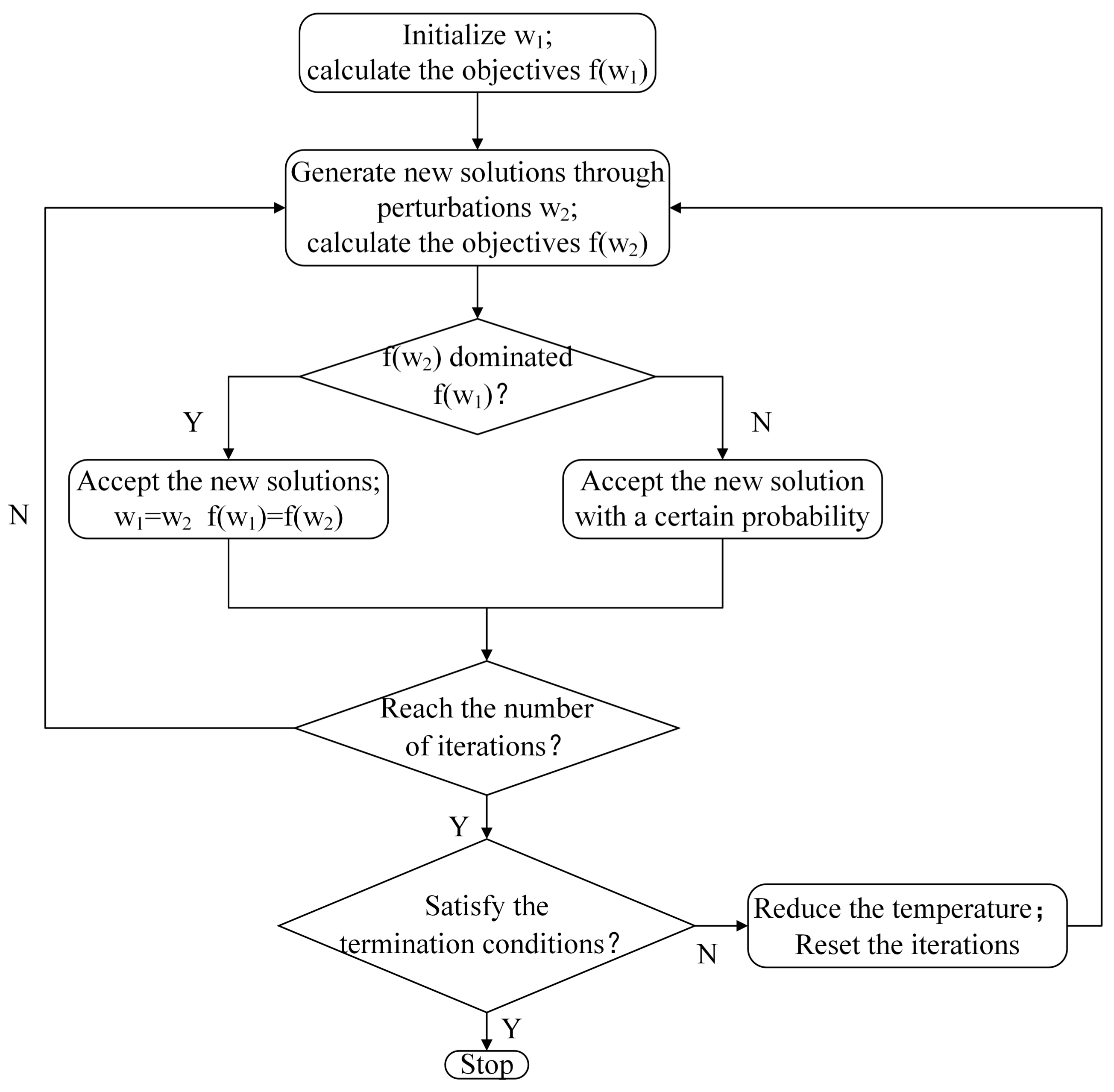
In order to address the complexity of problems, Kirkpatrick et al. [26] proposed simulate annealing (SA) first, which used the concept of the annealing process to seek for the optimal solution from the feasible domain. This algorithm iterates from a set of initial solutions with a high temperature, , and finishes with a final temperature, . The new solutions generated in each iteration are received with probability, , whose value is a function of the temperature. An annealing rate is used to determine the speed of annealing. The bigger value of means optimizing at a slower pace, which can approach the optimal solutions gradually.
Since there is more than one objective in this paper, a modified SA algorithm is developed to find appropriate Pareto solutions rather than getting one result used in a single objective environment. Based on the framework of Bandyopadhyay et al. [27], the multi-objective simulated annealing (MOSA) method is used to solve our problem. The procedure of MOSA is indicated in Figure 2.
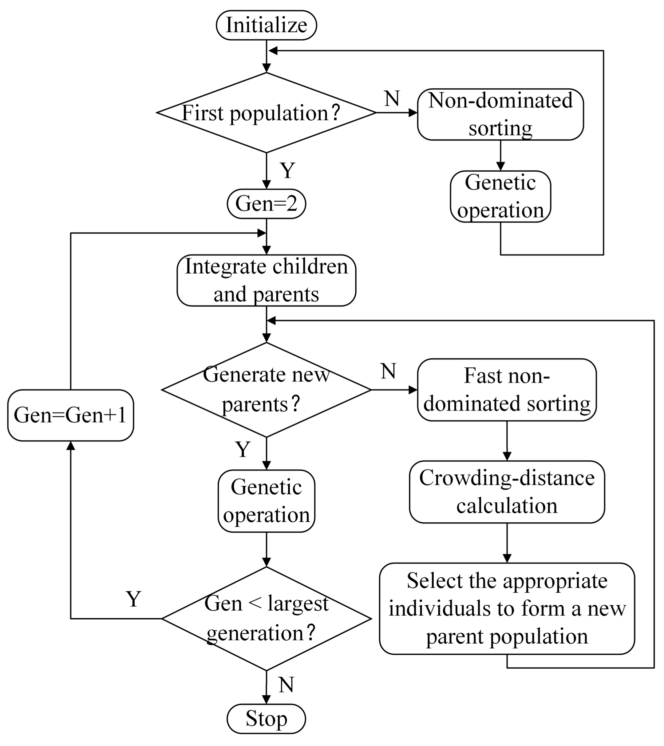
5.3. Non-Dominated Solution Genetic Algorithm
NSGA-II is an evolutionary algorithm, integrating a fast non-dominated sorting procedure and an elitist-preserving approach. The approach is widely used to solve the multi-objective problems effectively, and the procedure is shown as Figure 3. In this paper, the chromosome can be divided into three parts. The first part and second are binary variables, which denote the facilities and operation system (including transportation modes), respectively. The third part is the number of productions between facilities. The genetic operations are as follows.
- Genetic Operator 1:
- Randomly select two chromosomes;
- Exchange the facility locations of the two chromosomes;
- Change the second and third parts accordingly;
- Recalculate the objectives.
- Genetic Operator 2:
- Randomly select two chromosomes;
- Exchange the facility operation system of the two chromosomes;
- Change the first and third parts accordingly;
- Recalculate the objectives.
- Genetic Operator 3:
- Randomly select a chromosome;
- Change the number of transportation production;
- Change the first and second parts accordingly;
- Recalculating the objectives.
6. Performance Measurement
In this subsection, we first tune the parameter values in NSGA-II and MOSA. Then, we make a comparison between the two proposed algorithms using three indices, mainly in two aspects: the distance from the true Pareto front and the diversity of the solutions. All these algorithms are coded in MATLAB R2014b and are conducted on a PC with a 3.90-GHz Intel Core CPU processor and 4 GB RAM memory.
6.1. Introduction of Indicators
Three indicators are introduced in this section for algorithms’ performance measurement, which have been widely adopted in previous studies. The first one is distance from reference set indicator . It is used to measure the ‘distance’ between the approximate Pareto front and the true Pareto front [28]. A smaller means the approach performs better. For an approximate non-dominated solution set A and a reference solution set R, is calculated by the following expression:
where presents the distance between solutions x (in set A) and y (in set R),
where M is the number of objectives and are minimum and maximum values of the i-th objective in set R, respectively.
More precisely, the reference set R in the indicator expression refers to the true Pareto front. However, it is extremely difficult to obtain the true Pareto front, especially for large-scale instances. In this situation, R is formed by the total solutions obtained from the two heuristics.
The second one is the average e-dominance D. For two given non-dominated solution sets , it is used to get the dominance relations between them [29]. The indicator D is defined below.
where represents the relation that solution y dominates solution x. , where means that all the solutions in A are dominated by the solutions in B and means the opposite. Both and should be calculated for sets A and B, and A is judged better than B in the set coverage indicator when .
The third one is maximum spread indicator . This indicator illustrates the spread performance of the non-dominated solution set [30]. It is calculated by comparing with the reference set R mentioned in the first indicator, and set A is considered to cover a wider range of objective values when the indicator achieves a larger value.
6.2. Parameter Tuning
The performance of MOSA partly depends on the parameter set in the algorithm, including population size, the initial temperature, iteration generations and the coefficient of cooling. Since parameters of the proposed heuristics should be tuned under appropriate scale problem firstly, in our study, our tuning scale combination is , , , . We consider all four parameters mentioned above and carry out 36 parameter combinations with the following values: , , , .
The exact Pareto fronts of these instances can be obtained with the -constraint method. Parameter analysis using the exact Pareto front as the reference set is desirable and accurate. For each instance combination, ten independent runs are implemented considering the probability randomness of the obtained results. The mean value of the distance from reference set indicator is calculated for each parameter combination.
The results are listed in Table 2, and we select the parameter combination with the smallest value for the MOSA, marked in bold, which is ; where is indicated in the following experiments, i.e., the parameters of MOSA are set as .
The parameters, population size, the number of generations, the probability of cross and the probability of mutation have an influence on the performance of NSGA-II. In this paper, we take the four parameters mentioned above into account and consider the 36 combinations with the following values: , , , . Similar to MOSA, the reference set is the true front obtained by the method of -constraint, and we get the best parameter combination through calculating the mean value of indicator . The results are listed in Table 3. The smallest indicator is . The best parameter combination of NSGA-II is set as .
6.3. Comparison of the Proposed Algorithms
In the computational experiments, we generate 108 instances in total. Among 108 instances, there are 36 small-sized instances with the parameter combinations: , , , ; 36 middle-scale instances with the following values: , , , ; 36 large-sized instances with the following parameters: , , , . Both NSGA-II and MOSA are applied to all 108 instance combinations. Each example is calculated ten times independently with ten random parameters’ combinations. For all the instances, the average results of ten independent runs are recorded, and we apply the three indicators to measure the performance of the algorithms. In addition, the average running time of each algorithm in every instance test is also recorded as an indicator, to evaluate the computational efficiency.
For instance combination, it is rather difficult or time-consuming to get the true front, so that we apply the solutions generated by the two heuristics to the reference set. The results of three indicators of three scales are listed in Table 4, Table 5 and Table 6, respectively.
From the previous description, the smaller the value of first indicator is, the better the algorithm is, and it is opposite for the remaining two indicators. For the small-scale problem shown in Table 4, NSGA-II and MOSA’s average values of the first indicator are , , which means NSGA-II is about 37.79% better than MOSA considering the indicator . Similarly, the mean values of NSGA-II and MOSA are and for the average e-dominance indicator. The values and are of the third indicator of the two algorithms. Additionally, the NSGA-II performs better, by about 64.61% and 3.89% for the second and third indicators. After taking the average value, we can find that NSGA-II is 35.43% better than MOSA considering the quality of solutions. As for the running times of the two algorithms, the mean times are 112.45 seconds and 137.62 seconds, respectively. The results reflect that NSGA-II is more efficient, about 18.29% faster than MOSA.
Concerning the middle-sized problem, the results of three indicators are listed in Table 5. As for the distance from the reference set indicator, the values of the two heuristics are 0.0143 and 0.0330; hence, NSGA-II performs better, by about 56.67%, than MOSA. We can find that the values of NSGA-II are smaller for the first index comparing every instance. While we use the average e-dominance indicator to evaluate the performance, the value of every MOSA instance is smaller, which means MOSA performs worse, and the means are 0.7399 and 0.1687 for NSGA-II and MOSA, respectively. NSGA-II is about 77.20% better overall for second indicator. While considering the third indicator, we can find there are only five instances, , , , , , whose value of MOSA is bigger. However, on average, 1.3501 and 1.2534 for NSGA-II and MOSA state that NSGA-II performs better about 7.16%. It is easy to get the mean value, 47.01%, which illustrates that NSGA-II is about 47.01% better than MOSA from the perspective of solutions. The average running time of 36 instances is 198.24 seconds for NSGA-II and is 370.88 seconds for MOSA. NSGA-II is about 46.55% faster than MOSA.
Likewise, the large-scale instance experiment has similar conclusions shown in Table 6. For the first and second indicators, MOSA is worse than NSGA-II for every instance. The mean values of the distance from the reference set indicator are 0.0160 and 0.0377 for the two algorithms, which state that the NSGA-II is about 57.56% better than MOSA. For the average e-dominance indicator, the average values are 0.7427 and 0.1714, respectively, which illustrates that MOSA is worse than NSGA-II by about 76.92%. Concerning the third indicator, we can find that there are only three instances, , , , whose value of MOSA is bigger. It is obvious that the NSGA-II is better for the mean values, which are 1.3365 and 1.2601 for NSGA-II and MOSA. When considering the quality of solutions, NSGA-II is on average46.73% better than MOSA for the three indicators. From the perspective of running time, the two algorithms’ running times are 215.92 and 442.92, respectively, which illustrates that NSGA-II is faster by about 51.25% than MOSA.
Considering the above description synthetically, the mean values of three indicators are 0.0137, 0.7151, 1.3532 for NSGA-II and 0.0293, 0.5746, 1.2777 for MOSA. The average running times of the two algorithms are 175.54 and 317.14 seconds, respectively. Furthermore, NSGA-II is about 43.06% better than MOSA on average for 108 instances in terms of the quality of solution. From the perspective of running time, NSGA-II is about 38.70% faster than MOSA.
7. Conclusions
In this paper, we study the GCLSC problem. Similar to E-commerce service, the GCLSC is divided into four parts including manufacture, first-class warehouse, second-class warehouse and customer point. Furthermore, the locations and number of manufacturer and customer points are known, and several candidate locations of facilities are available. Recycling happens between customer points and second-class warehouses. A bi-objective model with the chance constraint was proposed considering uncertain demand in this paper. From the perspective of customers, they are very concerned about the quality of goods and the logistics speed, as well as the performance on environmental protection, so one objective is to maximize the satisfaction, which consists of the logistics speed, quality of goods and the amount of recycling products in this paper. Recycling more products means that the contribution of enterprises to environmental protection is more remarkable, which will also improve the satisfaction of the customer. The other conflict objective is to minimize the total cost.
To find a trade-off relation between these two objectives, we establish a bi-objective mathematical programming model joined with the chance constraint. An approximation method is used to handle the chance constraint. Additionally, an exact -constraint method is introduced to obtain exact Pareto fronts for small-scale instances. Two heuristic algorithms, NSGA-II and MOSA, are proposed to solve the GCLSC problem efficiently, especially for middle- and large-scale instances. Computational experiments are conducted, and the results illustrate the efficiency of the algorithms. Additionally, we can conclude that NSGA-II performs better than MOSA in this problem. Our research solves the problem of GCLSC under certain demand and provides guidance for manufacturers.
Future research directions, as well as research limitations of this paper may cover the following aspects: (i) inventory constraint; inventory plays an important role when making the production plan; the mathematical model can be extended to be closer to the actual situation; (ii) it is also interesting to consider a decentralized supply chain, then it should be a two-stage decision problem where suppliers and retailers only consider their own costs and profits. In this way, the problem becomes a two-stage stochastic programming problem, and we can use a sample approximation approach to solve it.
Acknowledgments
This work was supported by the National Natural Science Foundation of China (NSFC) under Grants 71531011, 71428002, 71771048 and 71571134. Supported by the Fundamental Research Funds for the Central Universities.
Author Contributions
Ming Liu and Zhanguo Zhu conceived of and designed the experiments. Rongfan Liu performed the experiments. Rongfan Liu and Xiaoyi Man analyzed the data. Chengbin Chu contributed analysis tools. Rongfan Liu wrote the paper.
Conflicts of Interest
The authors declare no conflicts of interest.
References
- Lambert, D.M.; Cooper, M.C. Issues in supply chain management. Ind. Mark. Manag. 2000, 29, 65–83. [Google Scholar] [CrossRef]
- Govindan, K.; Soleimani, H.; Kannan, D. Reverse logistics and closed-loop supply chain: A comprehensive review to explore the future. Eur. J. Oper. Res. 2015, 240, 603–626. [Google Scholar] [CrossRef] [Green Version]
- Elbounjimi, M. Green closed-loop supply chain network design a literature review. Int. J. Oper. Logist. Manag. 2014, 3, 275–286. [Google Scholar]
- Wei, J.; Govindan, K.; Li, Y. Pricing and collecting decisions in a closed-loop supply chain with symmetric and asymmetric information. Comput. Oper. Res. 2015, 54, 257–265. [Google Scholar] [CrossRef]
- Zhang, L. A nonlinear complementarity model for supply chain network equilibrium. J. Ind. Manag. Optim. 2007, 3, 727–737. [Google Scholar] [CrossRef]
- Cardona-Valdés, Y.; Álvarez, A.; Ozdemir, D. A bi-objective supply chain design problem with uncertainty. Transp. Res. Part C 2011, 19, 821–832. [Google Scholar] [CrossRef]
- Pereira, J.; Vilá, M. A new model for supply chain network design with integrated assembly line balancing decisions. Int. J. Prod. Res. 2015, 54, 1–17. [Google Scholar] [CrossRef] [Green Version]
- Eskandarpour, M.; Dejax, P.; Péton, O. A large neighborhood search heuristic for supply chain network design. Comput. Oper. Res. 2017, 80, 23–37. [Google Scholar] [CrossRef]
- Habibi, M.K.K.; Battaia, O.; Cung, V.D. Collection-disassembly problem in reverse supply chain. Int. J. Prod. Econ. 2017, 183, 334–344. [Google Scholar] [CrossRef]
- Kannan, G.; Noorul, A.; Devika, M. Analysis of closed loop supply chain using genetic algorithm and particle swarm optimization. Int. J. Prod. Res. 2009, 47, 1175–1200. [Google Scholar] [CrossRef]
- Turki, S.; Didukh, S.; Sauvey, C.; Rezg, N. Optimization and analysis of a manufacturing remanufacturing transport warehousing system within a closed-loop supply chain. Sustainability 2017, 9, 561. [Google Scholar] [CrossRef]
- Bottani, E.; Casella, G. Minimization of the environmental emissions of closed-loop supply chains: A case study of returnable transport assets management. Sustainability 2018, 10, 329. [Google Scholar] [CrossRef]
- Zhao, R.; Liu, Y.; Zhang, Z.; Guo, S.; Tseng, M.; Wu, K. Enhancing Eco-Efficiency of Agro-Products’ Closed-Loop Supply Chain under the Belt and Road Initiatives: A System Dynamics Approach. Sustainability 2018, 10, 668. [Google Scholar] [CrossRef]
- Huynh, C.H.; So, K.C.; Gurnani, H. Managing a closed-loop supply system with random returns and a cyclic delivery schedule. Eur. J. Oper. Res. 2016, 255, 787–796. [Google Scholar] [CrossRef]
- Zohal, M.; Soleimani, H. Developing an ant colony approach for green closed-loop supply chain network design: A case study in gold industry. J. Clean. Prod. 2016, 133, 314–337. [Google Scholar] [CrossRef]
- Soleimani, H.; Govindan, K.; Saghafi, H.; Jafari, H. Fuzzy multi-objective sustainable and green closed-loop supply chain network design. Comput. Ind. Eng. 2017, 109, 191–203. [Google Scholar] [CrossRef]
- Liu, S.; Chang, Y. Manufacturers’ closed-loop orientation for green supply chain management. Sustainability 2017, 9, 222. [Google Scholar] [CrossRef]
- Kaya, O.; Urek, B. A mixed integer nonlinear programming model and heuristic solutions for location, inventory and pricing decisions in a closed loop supply chain. Comput. Oper. Res. 2016, 65, 93–103. [Google Scholar] [CrossRef]
- Fleischmann, M.; Bloemhof-Ruwaard, J.M.; Dekker, R. Quantitative models for reverse logistics: A review. Eur. J. Oper. Res. 1997, 103, 1–17. [Google Scholar] [CrossRef] [Green Version]
- Thierry, M.; Salomon, M.; Van Nunen, J. Strategie issues in product recovery management. Calif. Manag. Rev. 1995, 37, 114–135. [Google Scholar] [CrossRef]
- Lu, Z.; Bostel, N. A facility location model for logistics systems including reverse flows: The case of remanufacturing activities. Comput. Oper. Res. 2007, 34, 299–323. [Google Scholar] [CrossRef]
- Franca, R.B.; Jones, E.C.; Richards, C.N. Multi-objective stochastic supply chain modeling to evaluate tradeoffs between profit and quality. Int. J. Prod. Econ. 2010, 127, 292–299. [Google Scholar] [CrossRef]
- Ng, M.W. Distribution-free vessel deployment for liner shipping. Eur. J. Oper. Res. 2014, 238, 858–862. [Google Scholar] [CrossRef]
- Hillermeier, C. Nonlinear multiobjective optimization. J. Oper. Res. Soc. 1999, 51, 246–256. [Google Scholar]
- Liu, M.; Yang, D.; Su, Q.; Xu, L. Bi-objective approaches for home healthcare medical team planning and scheduling problem. Computat. Appl. Math. 2018, 1–32. [Google Scholar] [CrossRef]
- Kirkpatrick, S.; Gelatt, J.; Vecchi, M.P. Optimization by simulated annealing. Read. Comput. Vis. 1987, 220, 606–615. [Google Scholar]
- Bandyopadhyay, S.; Saha, S.; Maulik, U.; Deb, K. A simulated annealing-based multiobjective optimization algorithm: Amosa. IEEE Trans. Evolut. Comput. 2008, 12, 269–283. [Google Scholar] [CrossRef]
- Coello, C.A.C.; Cortés, N.C. Solving multiobjective optimization problems using an artificial immune system. Genet. Progr. Evolvable Mach. 2005, 6, 163–190. [Google Scholar] [CrossRef]
- Zitzler, E.; Thiele, L.; Laumanns, M.; Fonseca, C.M.; Fonseca, V.G.D. Performance assessment of multiobjective optimizers: An analysis and review. IEEE Trans. Evolut. Comput. 2003, 7, 117–132. [Google Scholar] [CrossRef]
- Zitzler, E.; Deb, K.; Thiele, L. Comparison of multiobjective evolutionary algorithms: Empirical results. Evolut. Comput. 2000, 8, 173–195. [Google Scholar] [CrossRef] [PubMed]
Figure 1.
A green closed loop supply chain considering recycling.
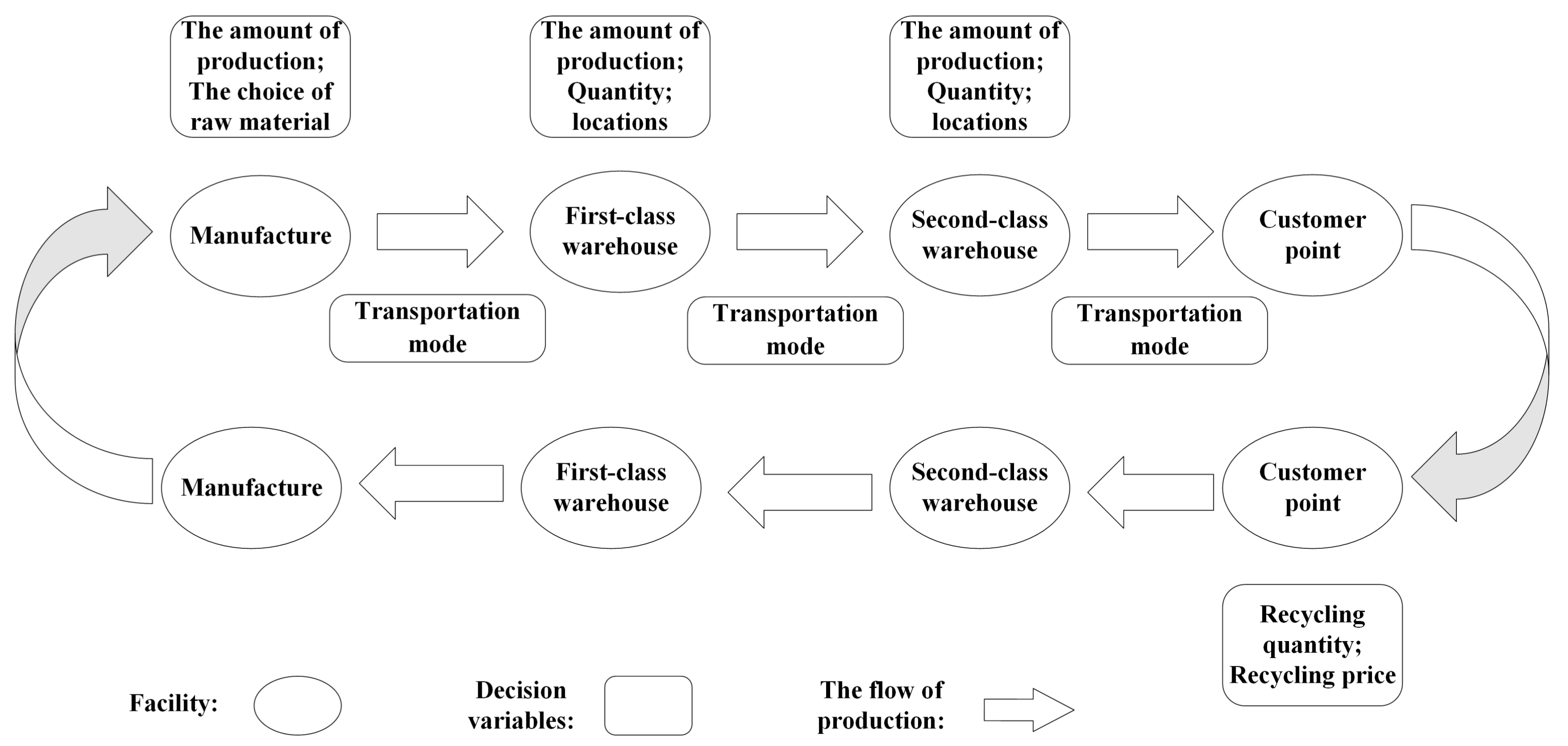
Figure 2.
The procedure of multi-objective simulated annealing (MOSA).

Figure 3.
The procedure of non-dominated sorting genetic algorithm (NSGA-II).


Table 1.
Summary of the dominant solutions.
| Solution ID | Objective 1 | Objective 2 | ||
|---|---|---|---|---|
| Cost | Satisfaction | |||
| (1) min Obj.2 | 84,995 | 0.00% | 31,913 | −54.89% |
| (2) Obj.1 ≤ 87177 | 85,292 | 0.35% | 48,263 | −31.78% |
| (3) Obj.1 ≤ 89177 | 87,292 | 2.70% | 54,593 | −22.83% |
| (4) Obj.1 ≤ 91177 | 89,394 | 5.18% | 56,103 | −20.70% |
| (5) Obj.1 ≤ 93177 | 91,394 | 7.53% | 57,621 | −18.55% |
| (6) Obj.1 ≤ 95177 | 93,393 | 9.88% | 58,951 | −16.67% |
| (7) Obj.1 ≤ 97177 | 95,394 | 12.23% | 60,111 | −15.04% |
| (8) Obj.1 ≤ 99177 | 97,395 | 14.59% | 61,386 | −13.23% |
| (9) Obj.1 ≤ 101177 | 99,395 | 16.94% | 62,521 | −11.63% |
| (10) Obj.1 ≤ 103177 | 101,395 | 19.30% | 63,578 | −10.13% |
| (11) Obj.1 ≤ 105177 | 103,395 | 21.65% | 64,358 | −9.03% |
| (12) Obj.1 ≤ 107177 | 105,395 | 24.00% | 64,928 | −8.23% |
| (13) Obj.1 ≤ 109177 | 107,395 | 26.35% | 65,738 | −7.08% |
| (14) Obj.1 ≤ 111177 | 109,412 | 28.73% | 66,368 | −6.19% |
| (15) Obj.1 ≤ 113177 | 111,412 | 31.08% | 66,848 | −5.51% |
| (16) Obj.1 ≤ 115177 | 113,411 | 33.43% | 67,328 | −4.83% |
| (17) Obj.1 ≤ 117177 | 115,412 | 35.79% | 67,808 | −4.16% |
| (18) Obj.1 ≤ 119177 | 117,412 | 38.14% | 68,258 | −3.52% |
| (19) Obj.1 ≤121177 | 119,412 | 40.49% | 68,678 | −2.93% |
| (20) Obj.1 ≤ 123177 | 121,451 | 42.89% | 69,068 | −2.37% |
| (21) Obj.1 ≤ 125177 | 123,452 | 45.25% | 69,398 | −1.91% |
| (22) Obj.1 ≤ 127177 | 125,453 | 47.60% | 69,728 | −1.44% |
| (23) Obj.1 ≤ 129177 | 127,547 | 50.06% | 70,058 | −0.98% |
| (24) Obj.1 ≤ 143177 | 141,617 | 66.62% | 70,268 | −0.68% |
| (25) Obj.1 ≤ 147177 | 145,638 | 71.35% | 70,328 | −0.59% |
| (26) Obj.1 ≤ 157177 | 156,399 | 84.01% | 70,478 | −0.38% |
| (27) Obj.1 ≤ 161177 | 160,408 | 88.73% | 70,538 | −0.30% |
| (28) Obj.1 ≤ 171177 | 171,157 | 101.37% | 70,688 | −0.08% |
| Ideal | 84,995 | 0.00% | 70,748 | 0.00% |
| Nadir | 175,177 | 106.10% | 31,913 | −54.89% |
Table 2.
Computational results for parameter tuning of MOSA.
| {200, 200, 20, 0.94} | 0.2382 | {250, 200, 20, 0.94} | 0.2308 |
| {200, 200, 20, 0.96} | 0.2184 | {250, 200, 20, 0.96} | 0.2390 |
| {200, 200, 20, 0.97} | 0.2175 | {250, 200, 20, 0.97} | 0.2243 |
| {200, 200, 25, 0.94} | 0.2473 | {250, 200, 25, 0.94} | 0.2535 |
| {200, 200, 25, 0.96} | 0.2243 | {250, 200, 25, 0.96} | 0.2236 |
| {200, 200, 25, 0.97} | 0.2343 | {250, 200, 25, 0.97} | 0.2210 |
| {200, 200, 30, 0.94} | 0.2594 | {250, 200, 30, 0.94} | 0.2359 |
| {200, 200, 30, 0.96} | 0.2251 | {250, 200, 30, 0.96} | 0.2300 |
| {200, 200, 30, 0.97} | 0.2149 | {250, 200, 30, 0.97} | 0.2103 |
| {200, 250, 20, 0.94} | 0.2183 | {250, 250, 20, 0.94} | 0.2467 |
| {200, 250, 20, 0.96} | 0.2289 | {250, 250, 20, 0.96} | 0.2169 |
| {200, 250, 20, 0.97} | 0.2028 | {250, 250, 20, 0.97} | 0.1961 |
| {200, 250, 25, 0.94} | 0.2433 | {250, 250, 25, 0.94} | 0.2588 |
| {200, 250, 25, 0.96} | 0.2340 | {250, 250, 25, 0.96} | 0.2513 |
| {200, 250, 25, 0.97} | 0.2396 | {250, 250, 25, 0.97} | 0.2052 |
| {200, 250, 30, 0.94} | 0.2341 | {250, 250, 30, 0.94} | 0.2255 |
| {200, 250, 30, 0.96} | 0.2028 | {250, 250, 30, 0.96} | 0.2196 |
| {200, 250, 30, 0.97} | 0.2140 | {250, 250, 30, 0.97} | 0.2022 |
Table 3.
Computational results for parameter tuning of NSGA-II.
| {150, 100, 0.8, 0.2} | 0.2335 | {200, 100, 0.8, 0.2} | 0.2159 |
| {150, 100, 0.8, 0.5} | 0.2220 | {200, 100, 0.8, 0.5} | 0.1939 |
| {150, 100, 0.8, 0.8} | 0.2060 | {200, 100, 0.8, 0.8} | 0.2076 |
| {150, 100, 0.5, 0.2} | 0.2228 | {200, 100, 0.5, 0.2} | 0.2286 |
| {150, 100, 0.5, 0.5} | 0.2318 | {200, 100, 0.5, 0.5} | 0.2030 |
| {150, 100, 0.5, 0.8} | 0.2047 | {200, 100, 0.5, 0.8} | 0.2148 |
| {150, 100, 0.2, 0.2} | 0.2682 | {200, 100, 0.2, 0.2} | 0.2277 |
| {150, 100, 0.2, 0.5} | 0.2398 | {200, 100, 0.2, 0.5} | 0.2471 |
| {150, 100, 0.2, 0.8} | 0.2550 | {200, 100, 0.2, 0.8} | 0.2288 |
| {150, 150, 0.8, 0.2} | 0.2161 | {200, 150, 0.8, 0.2} | 0.2035 |
| {150, 150, 0.8, 0.5} | 0.2027 | {200, 150, 0.8, 0.5} | 0.1896 |
| {150, 150, 0.8, 0.8} | 0.2078 | {200, 150, 0.8, 0.8} | 0.2086 |
| {150, 150, 0.5, 0.2} | 0.2227 | {200, 150, 0.5, 0.2} | 0.2066 |
| {150, 150, 0.5, 0.5} | 0.2027 | {200, 150, 0.5, 0.5} | 0.2011 |
| {150, 150, 0.5, 0.8} | 0.2141 | {200, 150, 0.5, 0.8} | 0.2099 |
| {150, 150, 0.2, 0.2} | 0.2291 | {200, 150, 0.2, 0.2} | 0.2346 |
| {150, 150, 0.2, 0.5} | 0.2374 | {200, 150, 0.2, 0.5} | 0.2362 |
| {150, 150, 0.2, 0.8} | 0.2384 | {200, 150, 0.2, 0.8} | 0.2359 |
Table 4.
Computational results for 36 small-scale instance combinations.
| Instance | NSGA-II (Referred to as A) | MOSA (Referred to as B) | ||||||
|---|---|---|---|---|---|---|---|---|
| C (AR) | MS | Time | C (BR) | MS | Time | |||
| {1, 3, 5, 12} | 0.0100 | 0.5226 | 1.3780 | 101.35 | 0.0122 | 0.3516 | 1.3382 | 72.18 |
| {1, 3, 5, 14} | 0.0098 | 0.7102 | 1.3916 | 105.45 | 0.0121 | 0.1864 | 1.2971 | 92.58 |
| {1, 3, 5, 16} | 0.0087 | 0.7758 | 1.4097 | 102.90 | 0.0120 | 0.1506 | 1.3378 | 161.64 |
| {1, 3, 6, 12} | 0.0095 | 0.6097 | 1.3816 | 107.83 | 0.0131 | 0.2388 | 1.3111 | 126.57 |
| {1, 3, 6, 14} | 0.0116 | 0.6521 | 1.4026 | 113.09 | 0.0149 | 0.2356 | 1.2812 | 125.13 |
| {1, 3, 6, 16} | 0.0077 | 0.6776 | 1.4003 | 108.02 | 0.0123 | 0.1969 | 1.2890 | 178.31 |
| {1, 3, 7, 12} | 0.0119 | 0.5649 | 1.3784 | 115.05 | 0.0146 | 0.3560 | 1.3562 | 88.83 |
| {1, 3, 7, 14} | 0.0074 | 0.5552 | 1.3763 | 121.84 | 0.0159 | 0.3320 | 1.3151 | 219.94 |
| {1, 3, 7, 16} | 0.0114 | 0.6031 | 1.3634 | 115.28 | 0.0120 | 0.3089 | 1.3592 | 205.14 |
| {1, 4, 5, 12} | 0.0061 | 0.3688 | 1.3985 | 104.74 | 0.0124 | 0.4832 | 1.3527 | 82.54 |
| {1, 4, 5, 14} | 0.0076 | 0.6874 | 1.3919 | 109.45 | 0.0118 | 0.2127 | 1.3039 | 105.54 |
| {1, 4, 5, 16} | 0.0113 | 0.5518 | 1.3738 | 103.75 | 0.0140 | 0.3601 | 1.3243 | 147.02 |
| {1, 4, 6, 12} | 0.0096 | 0.4977 | 1.3643 | 112.40 | 0.0130 | 0.2636 | 1.3638 | 75.85 |
| {1, 4, 6, 14} | 0.0081 | 0.5834 | 1.3940 | 117.15 | 0.0118 | 0.1564 | 1.3031 | 188.61 |
| {1, 4, 6, 16} | 0.0107 | 0.5454 | 1.3879 | 112.12 | 0.0140 | 0.3347 | 1.3327 | 194.39 |
| {1, 4, 7, 12} | 0.0122 | 0.7435 | 1.3474 | 120.78 | 0.0177 | 0.1640 | 1.2944 | 152.60 |
| {1, 4, 7, 14} | 0.0103 | 0.5582 | 1.3901 | 126.80 | 0.0129 | 0.2876 | 1.3510 | 182.62 |
| {1, 4, 7, 16} | 0.0122 | 0.7437 | 1.3684 | 121.01 | 0.0158 | 0.1206 | 1.3168 | 292.99 |
| {2, 3, 5, 12} | 0.0104 | 0.7024 | 1.3780 | 103.64 | 0.0202 | 0.1916 | 1.3272 | 57.68 |
| {2, 3, 5, 14} | 0.0093 | 0.7931 | 1.3718 | 103.94 | 0.0182 | 0.1313 | 1.3063 | 79.99 |
| {2, 3, 5, 16} | 0.0095 | 0.7972 | 1.3728 | 103.51 | 0.0183 | 0.2283 | 1.3173 | 131.24 |
| {2, 3, 6, 12} | 0.0104 | 0.7547 | 1.3912 | 106.48 | 0.0204 | 0.1547 | 1.2772 | 95.36 |
| {2, 3, 6, 14} | 0.0099 | 0.5850 | 1.3312 | 112.28 | 0.0192 | 0.3182 | 1.3198 | 73.52 |
| {2, 3, 6, 16} | 0.0089 | 0.6870 | 1.3809 | 112.62 | 0.0184 | 0.2066 | 1.3359 | 109.62 |
| {2, 3, 7, 12} | 0.0167 | 0.8011 | 1.3563 | 114.90 | 0.0235 | 0.1620 | 1.3316 | 105.89 |
| {2, 3, 7, 14} | 0.0119 | 0.5546 | 1.3791 | 117.38 | 0.0232 | 0.2494 | 1.3151 | 178.35 |
| {2, 3, 7, 16} | 0.0104 | 0.7362 | 1.3674 | 119.16 | 0.0172 | 0.1670 | 1.3453 | 185.41 |
| {2, 4, 5, 12} | 0.0135 | 0.5919 | 1.3251 | 104.55 | 0.0233 | 0.3522 | 1.3210 | 83.03 |
| {2, 4, 5, 14} | 0.0119 | 0.6937 | 1.3522 | 107.57 | 0.0217 | 0.2098 | 1.2818 | 107.09 |
| {2, 4, 5, 16} | 0.0106 | 0.6750 | 1.3548 | 109.36 | 0.0221 | 0.2688 | 1.3081 | 73.63 |
| {2, 4, 6, 12} | 0.0117 | 0.7808 | 1.3515 | 111.51 | 0.0186 | 0.2068 | 1.3365 | 128.20 |
| {2, 4, 6, 14} | 0.0131 | 0.6378 | 1.3580 | 116.10 | 0.0202 | 0.2124 | 1.3300 | 156.43 |
| {2, 4, 6, 16} | 0.0148 | 0.8224 | 1.3638 | 117.14 | 0.0235 | 0.0895 | 1.2997 | 184.92 |
| {2, 4, 7, 12} | 0.0130 | 0.8044 | 1.3779 | 119.57 | 0.0255 | 0.1459 | 1.2758 | 141.30 |
| {2, 4, 7, 14} | 0.0116 | 0.6986 | 1.3314 | 124.44 | 0.0220 | 0.2338 | 1.3377 | 146.16 |
| {2, 4, 7, 16} | 0.0121 | 0.7887 | 1.3862 | 125.07 | 0.0229 | 0.1726 | 1.3130 | 223.88 |
| Average | 0.0107 | 0.6627 | 1.3730 | 112.45 | 0.0172 | 0.2345 | 1.3196 | 137.62 |
Table 5.
Computational results for 36 middle-scale instance combinations.
| Instance | NSGA-II (Referred to as A) | MOSA (Referred to as B) | ||||||
|---|---|---|---|---|---|---|---|---|
| C (AR) | MS | Time | C (BR) | MS | Time | |||
| {2, 5, 8, 18} | 0.0115 | 0.7638 | 1.3794 | 168.05 | 0.0332 | 0.1743 | 1.2044 | 166.79 |
| {2, 5, 8, 20} | 0.0135 | 0.6159 | 1.3462 | 162.56 | 0.0312 | 0.2883 | 1.2577 | 297.51 |
| {2, 5, 8, 22} | 0.0164 | 0.9437 | 1.3561 | 170.55 | 0.0264 | 0.0270 | 1.2994 | 336.88 |
| {2, 5, 9, 18} | 0.0111 | 0.4888 | 1.3810 | 167.92 | 0.0247 | 0.4312 | 1.2873 | 286.48 |
| {2, 5, 9, 20} | 0.0184 | 0.7109 | 1.3638 | 175.74 | 0.0254 | 0.2256 | 1.3096 | 297.37 |
| {2, 5, 9, 22} | 0.0112 | 0.7458 | 1.3456 | 184.84 | 0.0226 | 0.1199 | 1.2834 | 343.98 |
| {2, 5, 10, 18} | 0.0127 | 0.6460 | 1.3829 | 180.20 | 0.0238 | 0.3029 | 1.2502 | 479.56 |
| {2, 5, 10, 20} | 0.0149 | 0.6520 | 1.3141 | 188.44 | 0.0230 | 0.1896 | 1.3165 | 418.46 |
| {2, 5, 10, 22} | 0.0188 | 0.7224 | 1.3286 | 196.97 | 0.0278 | 0.1469 | 1.3177 | 503.24 |
| {2, 6, 8, 18} | 0.0173 | 0.8583 | 1.3028 | 161.83 | 0.0283 | 0.1150 | 1.3225 | 317.92 |
| {2, 6, 8, 20} | 0.0171 | 0.7302 | 1.3831 | 171.46 | 0.0382 | 0.2119 | 1.2709 | 429.53 |
| {2, 6, 8, 22} | 0.0148 | 0.4792 | 1.2774 | 177.64 | 0.0277 | 0.3553 | 1.2837 | 415.91 |
| {2, 6, 9, 18} | 0.0175 | 0.8452 | 1.3112 | 175.90 | 0.0275 | 0.0766 | 1.2536 | 392.62 |
| {2, 6, 9, 20} | 0.0147 | 0.7081 | 1.3529 | 183.90 | 0.0388 | 0.2099 | 1.2561 | 398.30 |
| {2, 6, 9, 22} | 0.0147 | 0.7445 | 1.3947 | 191.79 | 0.0252 | 0.0740 | 1.2567 | 476.39 |
| {2, 6, 10, 18} | 0.0105 | 0.7796 | 1.3936 | 190.11 | 0.0289 | 0.0654 | 1.2302 | 459.14 |
| {2, 6, 10, 20} | 0.0170 | 0.6724 | 1.3733 | 199.59 | 0.0326 | 0.2308 | 1.2338 | 517.90 |
| {2, 6, 10, 22} | 0.0217 | 0.9453 | 1.3682 | 228.69 | 0.0460 | 0.0453 | 1.2156 | 402.23 |
| {3, 5, 8, 18} | 0.0185 | 0.8342 | 1.3292 | 170.68 | 0.0374 | 0.1462 | 1.1944 | 234.35 |
| {3, 5, 8, 20} | 0.0154 | 0.7669 | 1.2929 | 180.07 | 0.0291 | 0.1356 | 1.3191 | 251.36 |
| {3, 5, 8, 22} | 0.0178 | 0.7820 | 1.3631 | 195.66 | 0.0404 | 0.1127 | 1.2365 | 351.81 |
| {3, 5, 9, 18} | 0.0119 | 0.8291 | 1.4044 | 193.84 | 0.0415 | 0.1375 | 1.1971 | 305.07 |
| {3, 5, 9, 20} | 0.0079 | 0.6072 | 1.4040 | 206.17 | 0.0234 | 0.2614 | 1.2466 | 462.42 |
| {3, 5, 9, 22} | 0.0131 | 0.6965 | 1.3766 | 217.64 | 0.0392 | 0.1750 | 1.1405 | 383.77 |
| {3, 5, 10, 18} | 0.0111 | 0.6226 | 1.3055 | 221.22 | 0.0375 | 0.3092 | 1.2879 | 309.20 |
| {3, 5, 10, 20} | 0.0093 | 0.6916 | 1.3861 | 225.92 | 0.0299 | 0.2059 | 1.2501 | 453.90 |
| {3, 5, 10, 22} | 0.0112 | 0.7246 | 1.3671 | 215.32 | 0.0284 | 0.1739 | 1.2863 | 466.66 |
| {3, 6, 8, 18} | 0.0185 | 0.8622 | 1.3412 | 497.96 | 0.0434 | 0.0309 | 1.2928 | 315.60 |
| {3, 6, 8, 20} | 0.0101 | 0.8339 | 1.3027 | 173.53 | 0.0304 | 0.1372 | 1.2529 | 309.32 |
| {3, 6, 8, 22} | 0.0135 | 0.8259 | 1.3898 | 180.01 | 0.0408 | 0.1159 | 1.1954 | 352.42 |
| {3, 6, 9, 18} | 0.0058 | 0.5509 | 1.3948 | 178.04 | 0.0269 | 0.1759 | 1.1632 | 393.94 |
| {3, 6, 9, 20} | 0.0102 | 0.6675 | 1.2766 | 182.85 | 0.0352 | 0.1705 | 1.2190 | 353.93 |
| {3, 6, 9, 22} | 0.0182 | 0.9771 | 1.3945 | 190.94 | 0.0479 | 0.0000 | 1.2074 | 414.19 |
| {3, 6, 10, 18} | 0.0175 | 0.8455 | 1.3340 | 193.24 | 0.0447 | 0.1178 | 1.2712 | 224.56 |
| {3, 6, 10, 20} | 0.0164 | 0.5859 | 1.3144 | 212.44 | 0.0410 | 0.3086 | 1.2279 | 401.46 |
| {3, 6, 10, 22} | 0.0143 | 0.8788 | 1.2704 | 225.04 | 0.0378 | 0.0698 | 1.2865 | 427.43 |
| Average | 0.0143 | 0.7399 | 1.3501 | 198.24 | 0.0330 | 0.1687 | 1.2534 | 370.88 |
Table 6.
Computational results for 36 large-scale instance combinations.
| Instance | NSGA-II (Referred to as A) | MOSA (Referred to as B) | ||||||
|---|---|---|---|---|---|---|---|---|
| C (AR) | MS | Time | C (BR) | MS | Time | |||
| {2, 5, 9, 24} | 0.0208 | 0.8480 | 1.3020 | 185.78 | 0.0353 | 0.1116 | 1.3027 | 291.55 |
| {2, 5, 9, 26} | 0.0159 | 0.7381 | 1.3560 | 193.37 | 0.0332 | 0.1353 | 1.2413 | 438.01 |
| {2, 5, 9, 28} | 0.0120 | 0.7386 | 1.3648 | 199.57 | 0.0289 | 0.1144 | 1.2652 | 503.86 |
| {2, 5, 10, 24} | 0.0125 | 0.5849 | 1.3274 | 198.00 | 0.0262 | 0.3069 | 1.2574 | 441.82 |
| {2, 5, 10, 26} | 0.0164 | 0.6745 | 1.3577 | 206.27 | 0.0286 | 0.2453 | 1.3129 | 491.11 |
| {2, 5, 10, 28} | 0.0152 | 0.5364 | 1.3613 | 224.37 | 0.0256 | 0.3591 | 1.2763 | 530.42 |
| {2, 5, 11, 24} | 0.0199 | 0.7814 | 1.3271 | 222.04 | 0.0246 | 0.1697 | 1.3011 | 540.14 |
| {2, 5, 11, 26} | 0.0267 | 0.8926 | 1.3170 | 233.84 | 0.0397 | 0.0781 | 1.2840 | 531.98 |
| {2, 5, 11, 28} | 0.0101 | 0.7059 | 1.3839 | 242.92 | 0.0265 | 0.2386 | 1.2957 | 640.47 |
| {2, 6, 9, 24} | 0.0158 | 0.7523 | 1.3826 | 194.49 | 0.0290 | 0.1382 | 1.2593 | 476.12 |
| {2, 6, 9, 26} | 0.0112 | 0.6075 | 1.3189 | 201.12 | 0.0246 | 0.2200 | 1.2975 | 463.04 |
| {2, 6, 9, 28} | 0.0162 | 0.8251 | 1.3521 | 209.27 | 0.0394 | 0.0692 | 1.1945 | 440.44 |
| {2, 6, 10, 24} | 0.0114 | 0.7019 | 1.3551 | 207.88 | 0.0278 | 0.1611 | 1.2404 | 591.58 |
| {2, 6, 10, 26} | 0.0134 | 0.6143 | 1.3423 | 216.56 | 0.0298 | 0.1410 | 1.2860 | 464.02 |
| {2, 6, 10, 28} | 0.0222 | 0.6362 | 1.3341 | 226.15 | 0.0320 | 0.1470 | 1.2786 | 744.03 |
| {2, 6, 11, 24} | 0.0156 | 0.7165 | 1.3543 | 223.49 | 0.0309 | 0.2354 | 1.2624 | 576.32 |
| {2, 6, 11, 26} | 0.0232 | 0.8749 | 1.3110 | 233.66 | 0.0449 | 0.0567 | 1.2649 | 603.27 |
| {2, 6, 11, 28} | 0.0205 | 0.5352 | 1.3151 | 245.32 | 0.0404 | 0.4110 | 1.2916 | 662.85 |
| {3, 5, 9, 24} | 0.0096 | 0.7493 | 1.3123 | 188.10 | 0.0292 | 0.1870 | 1.2786 | 361.94 |
| {3, 5, 9, 26} | 0.0123 | 0.8378 | 1.2840 | 206.80 | 0.0318 | 0.0767 | 1.3151 | 460.95 |
| {3, 5, 9, 28} | 0.0128 | 0.6184 | 1.3509 | 206.19 | 0.0313 | 0.2687 | 1.2126 | 510.66 |
| {3, 5, 10, 24} | 0.0174 | 0.6621 | 1.3612 | 201.38 | 0.0410 | 0.2218 | 1.2301 | 485.29 |
| {3, 5, 10, 26} | 0.0151 | 0.4228 | 1.2622 | 210.86 | 0.0323 | 0.4506 | 1.3129 | 526.35 |
| {3, 5, 10, 28} | 0.0099 | 0.8439 | 1.3591 | 220.27 | 0.0304 | 0.1188 | 1.2751 | 530.91 |
| {3, 5, 11, 24} | 0.0146 | 0.8410 | 1.3088 | 216.80 | 0.0469 | 0.1239 | 1.2809 | 539.27 |
| {3, 5, 11, 26} | 0.0147 | 0.6601 | 1.3197 | 228.60 | 0.0402 | 0.2437 | 1.3063 | 577.52 |
| {3, 5, 11, 28} | 0.0121 | 0.6361 | 1.3844 | 239.59 | 0.0324 | 0.2553 | 1.2630 | 598.84 |
| {3, 6, 9, 24} | 0.0146 | 0.8087 | 1.3377 | 195.46 | 0.0403 | 0.1666 | 1.2761 | 450.28 |
| {3, 6, 9, 26} | 0.0136 | 0.8042 | 1.3520 | 202.87 | 0.0402 | 0.0428 | 1.2094 | 509.48 |
| {3, 6, 9, 28} | 0.0158 | 0.8969 | 1.3518 | 211.26 | 0.0440 | 0.0419 | 1.2602 | 515.24 |
| {3, 6, 10, 24} | 0.0187 | 0.8761 | 1.3509 | 212.39 | 0.0604 | 0.0501 | 1.2194 | 76.46 |
| {3, 6, 10, 26} | 0.0175 | 0.8285 | 1.2685 | 220.61 | 0.0398 | 0.1734 | 1.2286 | 89.00 |
| {3, 6, 10, 28} | 0.0176 | 0.9089 | 1.3618 | 230.55 | 0.0673 | 0.0869 | 1.1285 | 49.08 |
| {3, 6, 11, 24} | 0.0246 | 0.9521 | 1.3407 | 227.82 | 0.0746 | 0.0258 | 1.1803 | 79.01 |
| {3, 6, 11, 26} | 0.0234 | 0.8519 | 1.3065 | 239.19 | 0.0599 | 0.0981 | 1.2557 | 67.59 |
| {3, 6, 11, 28} | 0.0129 | 0.7744 | 1.3402 | 250.23 | 0.0463 | 0.1992 | 1.2193 | 86.22 |
| Average | 0.0160 | 0.7427 | 1.3365 | 215.92 | 0.0377 | 0.1714 | 1.2601 | 442.92 |
© 2018 by the authors. Licensee MDPI, Basel, Switzerland. This article is an open access article distributed under the terms and conditions of the Creative Commons Attribution (CC BY) license (http://creativecommons.org/licenses/by/4.0/).
Share and Cite
MDPI and ACS Style
Liu, M.; Liu, R.; Zhu, Z.; Chu, C.; Man, X. A Bi-Objective Green Closed Loop Supply Chain Design Problem with Uncertain Demand. Sustainability 2018, 10, 967. https://doi.org/10.3390/su10040967
AMA Style
Liu M, Liu R, Zhu Z, Chu C, Man X. A Bi-Objective Green Closed Loop Supply Chain Design Problem with Uncertain Demand. Sustainability. 2018; 10(4):967. https://doi.org/10.3390/su10040967
Chicago/Turabian StyleLiu, Ming, Rongfan Liu, Zhanguo Zhu, Chengbin Chu, and Xiaoyi Man. 2018. "A Bi-Objective Green Closed Loop Supply Chain Design Problem with Uncertain Demand" Sustainability 10, no. 4: 967. https://doi.org/10.3390/su10040967
Note that from the first issue of 2016, this journal uses article numbers instead of page numbers. See further details here.