A Systematic Cycle Time Reduction Procedure for Enhancing the Competitiveness and Sustainability of a Semiconductor Manufacturer

Abstract

Cycle time reduction plays an important role in improving the competitiveness and sustainability of a semiconductor manufacturer. However, in the past, cycle time reduction was usually unplanned owing to the lack of a systematic and quantitative procedure. To tackle this problem, a systematic procedure was established in this study for planning cycle time reduction actions to enhance the competitiveness and sustainability of a semiconductor manufacturer. First, some controllable factors that are influential to the job cycle time are identified. Subsequently, the relationship between the controllable factors and the job cycle time is fitted with a back propagation network. Based on this relationship, actions to shorten the job cycle time can be planned. The feasibility and effectiveness of an action have to be assessed before it can be taken in practice. An example containing the real data of hundreds of jobs has been used to illustrate the applicability of the proposed methodology. In addition, the financial benefits of the cycle time reduction action were analyzed, which provided the evidence that the proposed methodology enabled the sustainable development of the semiconductor manufacturer, since capital adequacy is very important in the semiconductor manufacturing industry.

1. Introduction

The cycle time (flow time, or manufacturing lead time) of a job is the time required for the job to go through the factory. Shortening the job cycle time is very important for a factory, at least for the following reasons:

(1)

Each job represents an opportunity cost for the factory. A long cycle time means it is difficult to convert the opportunity cost into profits in the short term.

(2)

Long job cycle times result in the accumulation of work-in-progress (WIP), which makes the shop floor management a challenging task.

(3)

In a semiconductor manufacturing factory, the risk that a wafer is contaminated increases if the cycle time is long.

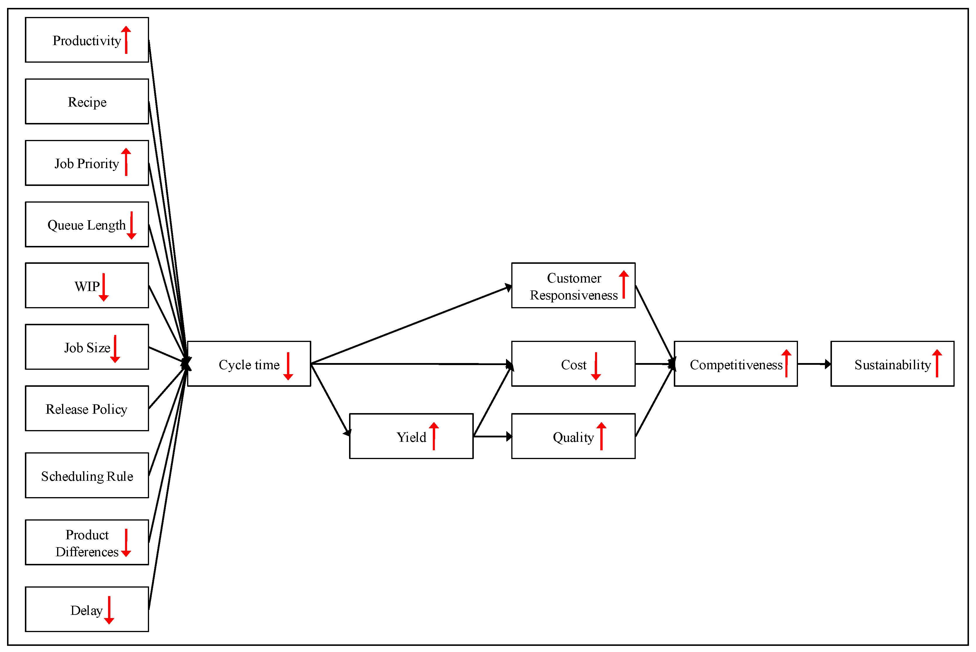
These issues are related with cycle time, cost, and yield (i.e., product quality). In fact, the three factors are not only the keys to the competitiveness of a semiconductor manufacturer [1,2,3], but also decisive factors for the sustainability of the semiconductor manufacturer. The conclusions of some relevant studies on the competitiveness and sustainability of a semiconductor manufacturer were summarized in Table 1. In the past, support from the government enabled the continued growth of semiconductor manufacturers in some regions, such as Taiwan and South Korea. After such support disappears, how to continue to maintain competitiveness and sustainability becomes a big problem. For example, not being able to push costs down further has forced many dynamic random access memory (DRAM) manufacturers to exit the market. The survived continue to reduce the job cycle time, so as to respond more quickly to changes in customer demand, and thus gain a competitive advantage [4]. A shorter job cycle time also means it is possible to commit an attractive due date to the customer. That helps to expand the market share and to ensure sustainability.

Table 1. Conclusions of some relevant studies on the competitiveness and sustainability of a semiconductor manufacturer.

Reference	Objective
Armstrong [5]	Four principles for competitive semiconductor manufacturing were proposed.
Jenkins et al. [6]	The importance of quality is stressed.Quality should be designed into products and processes.
Fulcher [7]	The accuracy of forecasting technology trends and emerging markets is important to the competitiveness of a semiconductor manufacturer.
Leachman [8]	Factors that influence competitive semiconductor manufacturing (CSM) were identified.
Peng and Chien [1]	Shortening cycle time, producing high-quality products, on-time delivery of orders, continual cost reductions, and improving efficiency were considered as the most direct and effective ways to create value for customers.
Walsh et al. [9]	The competitiveness and sustainability of a semiconductor manufacturer are closely related.
Liao and Hu [10]	Knowledge management is a decisive factor for a semiconductor manufacturer to develop and maintain its competitive advantage.
Chen [2]	Allocating more factory capacity to a product can change the yield learning process and enhance the competitiveness.
Chien and Zheng [11]	A semiconductor manufacturer has to constantly develop and employ the latest technology to maintain a competitive advantage.
Nakagawa et al. [12]	Distributors can create good cooperation and collaboration by mediates between semiconductor manufacturers and user companies.
Chen [3]	Cost competitiveness is a subjective concept that can be modeled with a fuzzy value.The long-term competitiveness can be assessed by observing the trend in the mid-term competitiveness.
Chen and Wang [13]	Productivity is crucial to the competitiveness of a semiconductor manufacturer.The long-term competitiveness is the key to the sustainability of a factory.

Table 1. Conclusions of some relevant studies on the competitiveness and sustainability of a semiconductor manufacturer.

Reference	Objective
Armstrong [5]	Four principles for competitive semiconductor manufacturing were proposed.
Jenkins et al. [6]	The importance of quality is stressed.Quality should be designed into products and processes.
Fulcher [7]	The accuracy of forecasting technology trends and emerging markets is important to the competitiveness of a semiconductor manufacturer.
Leachman [8]	Factors that influence competitive semiconductor manufacturing (CSM) were identified.
Peng and Chien [1]	Shortening cycle time, producing high-quality products, on-time delivery of orders, continual cost reductions, and improving efficiency were considered as the most direct and effective ways to create value for customers.
Walsh et al. [9]	The competitiveness and sustainability of a semiconductor manufacturer are closely related.
Liao and Hu [10]	Knowledge management is a decisive factor for a semiconductor manufacturer to develop and maintain its competitive advantage.
Chen [2]	Allocating more factory capacity to a product can change the yield learning process and enhance the competitiveness.
Chien and Zheng [11]	A semiconductor manufacturer has to constantly develop and employ the latest technology to maintain a competitive advantage.
Nakagawa et al. [12]	Distributors can create good cooperation and collaboration by mediates between semiconductor manufacturers and user companies.
Chen [3]	Cost competitiveness is a subjective concept that can be modeled with a fuzzy value.The long-term competitiveness can be assessed by observing the trend in the mid-term competitiveness.
Chen and Wang [13]	Productivity is crucial to the competitiveness of a semiconductor manufacturer.The long-term competitiveness is the key to the sustainability of a factory.

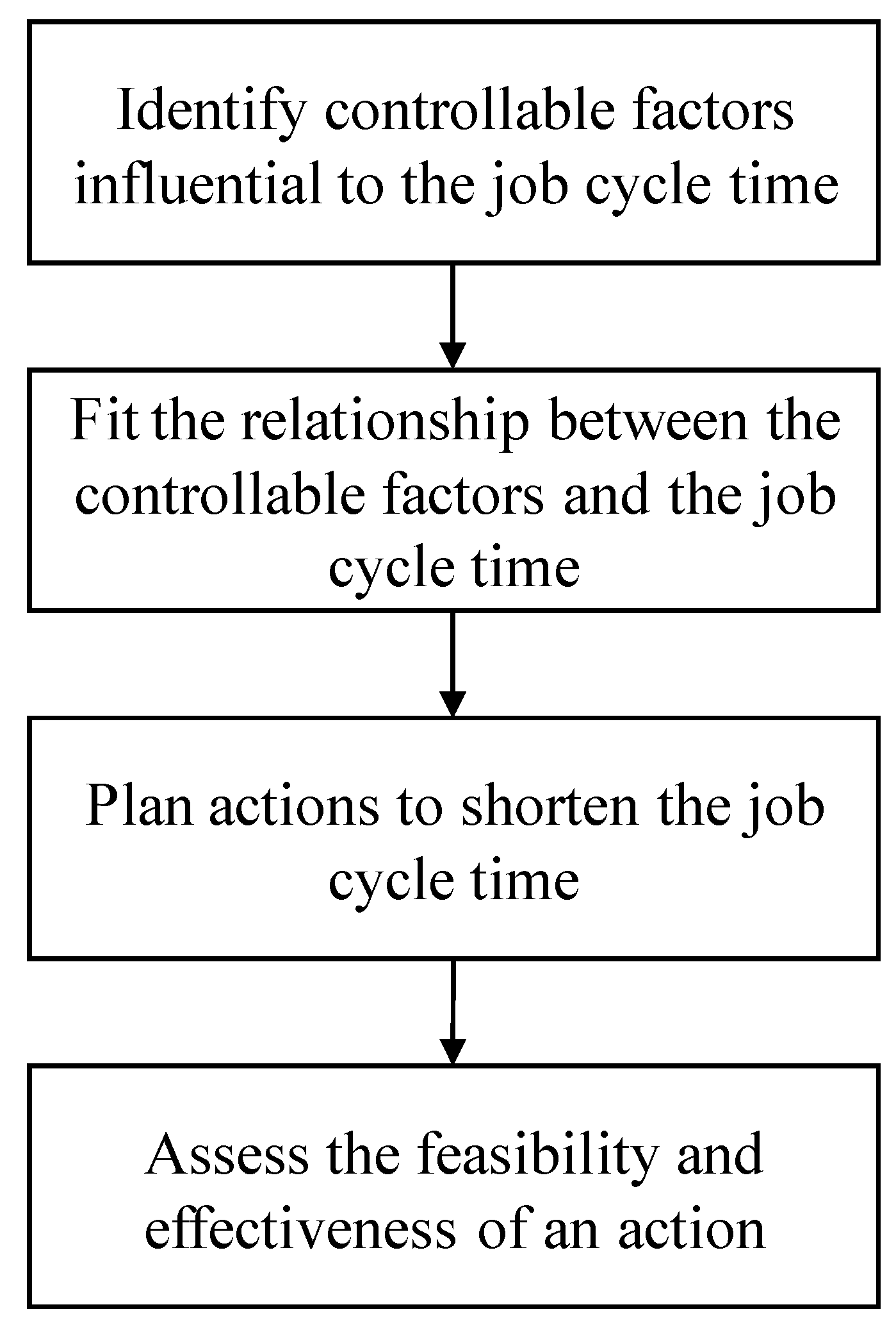
However, in the past, cycle time reduction was usually unplanned owing to the lack of a systematic and quantitative procedure. To tackle this problem, this study aims to establish a systematic procedure for planning cycle time reduction actions to enhance the competitiveness and sustainability of a semiconductor manufacturer (see Figure 1). To this end, a four-step procedure is followed:

(1)

Identify factors that are influential to the job cycle time and are controllable: The cycle time of a job is subject to capacity constraints, the factory congestion level, the quality of job scheduling, and many other factors [14]. However, these factors must be operable to be useful, and this step is to adjust such operable factors so that the job cycle time can be shortened.

(2)

Fit the relationship between the controllable factors and the job cycle time: The existing methods for fitting the relationship between the controllable factors and the job cycle time can be divided into several categories: probability-based statistical methods, case-based reasoning (CBR), artificial neural networks (ANNs), simulation, and hybrid approaches. A recent literature review on these methods can be seen in Chen and Wang [15]. In this study, an ANN is used. A number of studies have shown that linear methods are incapable of estimating the job cycle time [4]. Nonlinear method, such as ANNs, are more appropriate to estimate the job cycle time.

(3)

Plan actions to shorten the job cycle time: We can take actions to change the attributes and processing order of a job, or the size of the storage area to adjust the values of the controllable factors, which shortens the job cycle time according to the mechanism fitted in (2). In addition, adopting a more effective scheduling rule has also been shown to shorten the cycle time [16]; however, it requires extensive and time-consuming evaluation, usually after a series of simulation experiments.

(4)

Assess the feasibility and effectiveness of an action: We can compare the new values of the controllable factors to those that have been used in the past to assess the feasibility and effectiveness of an action. To this end, two indexes, based on the mean absolute percentagedeviation (MAPD) between the target values and the historical/original values, have been proposed.

The remainder of this paper is organized as follows. Section 2 is divided into four parts; each of them details a step of the proposed methodology. To illustrate the applicability of the proposed methodology, a real case from a semiconductor manufacturing factory is used. Based on the application results, the advantages and/or disadvantages of the proposed methodology are discussed. Based on them, some points are concluded. At last, some directions for future exploration are also given in the last section.

Figure 1. The motive for the proposed methodology.

Figure 1. The motive for the proposed methodology.

2. Methodology

The proposed methodology includes the following steps, as illustrated in Figure 2.

Figure 2. The procedure of the proposed methodology.

Figure 2. The procedure of the proposed methodology.

2.1. Identify Controllable Factors Influential to the Job Cycle Time

The first step of model building often consists of selecting a parsimonious set of independent variables from a pool of candidate independent variables. There are a number of factors that are influential to the job cycle time. These factors can be divided into the following categories [14,17]:

(1)

WIP in the factory: As the monthly capacity of a semiconductor manufacturing factory is normally fixed, the WIP in the factory is usually determined by the release plan. However, after receiving an order, a foundry has to release the corresponding jobs into the factory as soon as possible. For this reason, the release plan and WIP are not under the control of a foundry.

(2)

The workload of a factory, which can be measured in terms of the utilization of the bottleneck machines in the factory.

(3)

The queue lengths before machines, especially bottleneck machines, which is one of the main factors leading to a long cycle time. The queue length before a machine depends on the good, or bad, of the scheduling performance, and can be controlled by adjusting the buffer size before the machine.

(4)

Job attributes: The size, priority, and total processing time of a job directly affects the job’s cycle time. In addition, the number of re-entrances to machines is proportional to the number of times that a job is queued, and therefore is also a decisive factor to the job’s cycle time.

(5)

Lateness information: The lateness of some recently completed jobs is information of great reference value for estimating the job cycle time.

(6)

Worker productivity, which usually follows a learning process. Despite the short-term productivity can be enhanced through incentives or rewards, the long-term trend is very difficult to change. A detailed discussion on this can be seen in Chen and Wang [13].

To select from these candidate independent variables, stepwise and backward elimination are two common statistical techniques in regression analysis. However, Li [18] has shown that backward elimination is slightly better than stepwise elimination. For this reason, backward elimination is applied in this study to filter out the decisive factors to estimate the job cycle time:

(1)

Start with all candidate variables.

(2)

Test the deletion of each variable to optimize a fitness indicator, e.g., F-test, t-test, adjusted R², Akaike information criterion, Bayesian information criterion, Mallows’s C_p, and false discovery rate.

(3)

Delete the variable that can improve the fitness most.

(4)

Repeat this process until no further improvement can be achieved.

2.2. Fit the Relationship between the Controllable Variables and the Job Cycle Time

In a wafer fabrication factory, the relationship between the controllable factors and the job cycle time is undoubtedly nonlinear [4]. BPN is a well-known tool for fitting nonlinear relationships, so is a very good choice to fit the relationship.

In the proposed methodology, a BPN is established to fit the relationship between the controllable variables and the job cycle time. The configuration of the BPN is as follows (see Figure 3):

(1)

Network inputs: Inputs to the BPN are the values of the K controllable factors, indicated with x_jk , k = 1–K. However, the values of these attributes have to be normalized to be within 0.1–0.9 to facilitate the following computation [19].

(2)

Hidden layers: Only a single hidden layer is used. The number of nodes in the hidden layer is 2K.

(3)

Activation/transformation function: For the input layer, the linear activation function keeping the inputted value is used.

f(x_jk) = x_jk

(1)

(4)

while for the other layers, the hyperbolic tangent sigmoid function is used, and the output ranges from 0 to 1:

(2)

(5)

Network output (o_j): the estimated cycle time of job j.

(6)

Training method: There are several methods for training a BPN, such as the gradient descent algorithm, the conjugate gradient algorithm, the Levenberg-Marquardt algorithm, and others. The gradient descent algorithm is slow, while the Levenberg-Marquardt algorithm may over-fit for the testing data [20]. In this study, the gradient descent algorithm is applied.

(7)

Learning rate (η): 0.1.

(8)

Number of epochs: 15000.

(9)

Convergence criteria: The BPN training stops if mean squared error (MSE) falls below 10⁻⁵ or 15000 epochs have been run:

(3)

where a_j is the cycle time of job j. N() is the normalization function.

Figure 3. The architecture of the BPN.

Figure 3. The architecture of the BPN.

Inputs to the BPN are directly passed to the inputs nodes. After being weighted, they are passed to each hidden-layer node, summed, compared with the threshold on the node, and transformed. Finally, the output from the hidden-layer node is generated as

(4)

(5)

(6)

where h_l is the output from hidden-layer node l; is the threshold on this node; is the weight of the connection between input node k and hidden-layer node l. h_l is passed to the output node in the same way, and finally the network output, i.e., the cycle time estimate of job j, is generated as

(7)

where

(8)

(9)

where is the threshold on the output node; is the weight of the connection between hidden-layer node l and the output node.

After comparing the network output with the actual cycle time, the estimation error can be derived. The gradient descent algorithm passes the estimation error backward to adjust the thresholds and connection weights in an iterative manner:

(10)

(11)

(12)

(13)

(14)

(15)

where , , , and indicate the adjustments that should be made to the corresponding parameters. η is the learning rate.

2.3. Plan Actions to Shorten the Job Cycle Time

There are many references to provide evidence that various actions can be taken to shorten the job cycle time. Ng et al. [21] identified factors in the purchasing and transportation processes that influence a firm’s ability to reduce the cycle time. Browning [22] discussed some of the challenges that impede efforts to reduce the job cycle time, including inefficient distribution of personnel and resources, unstable product requirements, the existence of long and various activity pipelines, lack of activity coordination, highly interdependent or coupled activities, and overly ambitious initial schedules. Seth and Gupta [23] proved that value stream mapping (VSM) is effective in identifying and eliminating wastes in a factory with similar or identical product routings, which also helps to shorten the job cycle time. Better scheduling rules have been shown to reduce the job cycle time in simulation experiments [16,24]; however, a long period of evaluation and system adjustments needs to be gone through before the new scheduling rule to be fully online. Nazzal et al. [25] tried to quantify the economic impact of reducing the job cycle time. First, the bottleneck machines in a semiconductor manufacturing factory that have a significant impact on the job cycle time were identified. Then, the production capacities of the bottleneck machines were increased. However, capacity expansion is a time-consuming task, and requires the cooperation of equipment suppliers.

In short, the following actions may reduce the job cycle time, and are relatively easy to take:

(1)

Lower the WIP level in the factory: The most effective way to lower the WIP level in a factory is through capacity expansion; however, that is not easy except for a new factory. Another solution is to slow down the pace at which new jobs are released into the factory. However, that is difficult sometimes, especially in a foundry. An alternative is to accelerate the progresses of jobs that are almost done.

(2)

Shorten the queue lengths, especially before bottleneck machines: The performance of a manufacturing system is usually determined by bottleneck machines. For this reason, bottleneck machines are usually the targets of improvement. However, bottlenecks may shift, and therefore should be detected continuously. The queue lengths before bottleneck machines can be shortened by controlling the outputs from the upstream machines. However, a semiconductor manufacturing factory is a reentrant production system, in which downstream machines may become upstream machines, and vice versa. In addition, narrowing the buffer space can achieve a similar effect. Scheduling using some fluctuation smoothing rules was also shown to be helpful for this purpose [26].

(3)

Control the delay of jobs: A delayed job means it spent more time than expected in the semiconductor manufacturing factory. Within this extra time, the job continues to compete for the capacities, and to join the queues before machines, thus lengthening the cycle times of the other jobs. For this reason, controlling the delay of jobs is a critical task. To this end, one approach is to accelerate the progresses of jobs that are almost late. In addition, the job size is inversely proportional to the required setups, and is also influential to the cycle time and delay [27]. Therefore, changing the job size may help to control the delay [28,29,30]

The corresponding actions in these categories were summarized in Table 2.

However, Browning [22] warned that many seemingly feasible cycle time reduction solutions have adverse side effects. Therefore, any cycle time reduction action must pass the feasibility assessment, as described in the next section.

Table 2. Some possible actions for reducing the job cycle time.

Category	Possible Actions
Lower the WIP level in the factory	Capacity expansion
	Slow down the pace of releasing new jobs
	Lower the factory utilization
	Accelerate jobs that are almost done
Shorten the queue lengths, especially before bottleneck machines	Narrow the buffer size
	Control the outputs from the upstream machines
	Schedule using fluctuation smoothing rules
Control the delay of jobs	Accelerate jobs that are almost late
	Reduce the job size

Table 2. Some possible actions for reducing the job cycle time.

Category	Possible Actions
Lower the WIP level in the factory	Capacity expansion
	Slow down the pace of releasing new jobs
	Lower the factory utilization
	Accelerate jobs that are almost done
Shorten the queue lengths, especially before bottleneck machines	Narrow the buffer size
	Control the outputs from the upstream machines
	Schedule using fluctuation smoothing rules
Control the delay of jobs	Accelerate jobs that are almost late
	Reduce the job size

2.4. Assess the Feasibility and Effectiveness of An Action

A cycle time reduction action is feasible if

(1)

The target values of the controllable variables have been used in the past, or at least are close to those used in the past. To guarantee this, the mean absolute percentage deviation (MAPD) between the target values and the historical values has to be less than a threshold θ₁:

(16)

(2)

Setting the controllable variables to the target values can indeed reduce the job cycle time, according to the BPN estimate.

(3)

The realizability of the cycle time reduction action has been approved by the relevant production control engineer.

In addition, a feasible cycle time reduction action is effective if it minimizes the MAPD between the target values and the original values of the controllable variables:

(17)

3. Illustrative Examples

To illustrate the application of the proposed methodology, the data of 120 jobs from a semiconductor manufacturing factory have been collected, including the attributes and cycle time of each job, the factory conditions when each job was released into the factory, and delay-related information (see Table 3). Except the cycle time, which is the dependent variable, all the other variables were filtered to remove uncontrollable ones.

Table 3. The collected variables.

Category	Variables
Job Attributes	Job size
	Cycle time
	Number of steps
	Number of reentraces
	Total processing time
	Due date
Factory Conditions	Factory WIP when a job is released
	Factory utilization of the day before a job is released
	Queue length before bottleneck machines when a job is released
	Queue length on the processing route of a job when the job is released
Delay-related Information	Delay
	Waiting time

Table 3. The collected variables.

Category	Variables
Job Attributes	Job size
	Cycle time
	Number of steps
	Number of reentraces
	Total processing time
	Due date
Factory Conditions	Factory WIP when a job is released
	Factory utilization of the day before a job is released
	Queue length before bottleneck machines when a job is released
	Queue length on the processing route of a job when the job is released
Delay-related Information	Delay
	Waiting time

After backward elimination of regression analysis, six controllable variables that were the most influential for the job cycle time were determined as: x_j1–the job size, x_j2–factory WIP, x_j3–the queue length before the bottleneck, x_j4–the queue length on the route, x_j5–the average waiting time, and x_j6–factory utilization, as shown in Table 4. The fitted regression equation is a_j = −373 + 5.273x_j1 + 1.834x_j2 + 1.220x_j3 – 1.853x_j4 +0.080x_j5 + 286x_j6. R² = 0.73 and adjusted R² = 0.72. The analysis of variance (ANOVA) results are shown in Table 5.

Table 4. The six controllable variables.

j	xj1 (pieces)	xj2 (jobs)	xj3 (jobs)	xj4 (jobs)	xj5 (hrs)	xj6	aj (hrs)
1	24	1223	158	807	99	0.842	953
2	23	1225	164	665	142	0.948	1248
3	25	1232	154	718	373	0.884	1299
4	23	1282	165	813	148	0.929	976
5	22	1352	182	760	389	0.931	1189
116	23	1322	154	664	82	0.930	1561
117	22	1292	156	805	209	0.803	1241
118	23	1173	157	791	111	0.801	859
119	24	1270	175	688	38	0.909	1148
120	22	1319	159	777	326	0.888	1285

Table 4. The six controllable variables.

j	xj1 (pieces)	xj2 (jobs)	xj3 (jobs)	xj4 (jobs)	xj5 (hrs)	xj6	aj (hrs)
1	24	1223	158	807	99	0.842	953
2	23	1225	164	665	142	0.948	1248
3	25	1232	154	718	373	0.884	1299
4	23	1282	165	813	148	0.929	976
5	22	1352	182	760	389	0.931	1189
116	23	1322	154	664	82	0.930	1561
117	22	1292	156	805	209	0.803	1241
118	23	1173	157	791	111	0.801	859
119	24	1270	175	688	38	0.909	1148
120	22	1319	159	777	326	0.888	1285

Table 5. ANOVA results.

	Degree of freedom	SS	MS	F	significance
Regression	6	3,687,846	614,641	52.14	2.58×10−30
Residuals	113	1,332,180	11,789
Sum	119	5,020,027

Table 5. ANOVA results.

	Degree of freedom	SS	MS	F	significance
Regression	6	3,687,846	614,641	52.14	2.58×10−30
Residuals	113	1,332,180	11,789
Sum	119	5,020,027

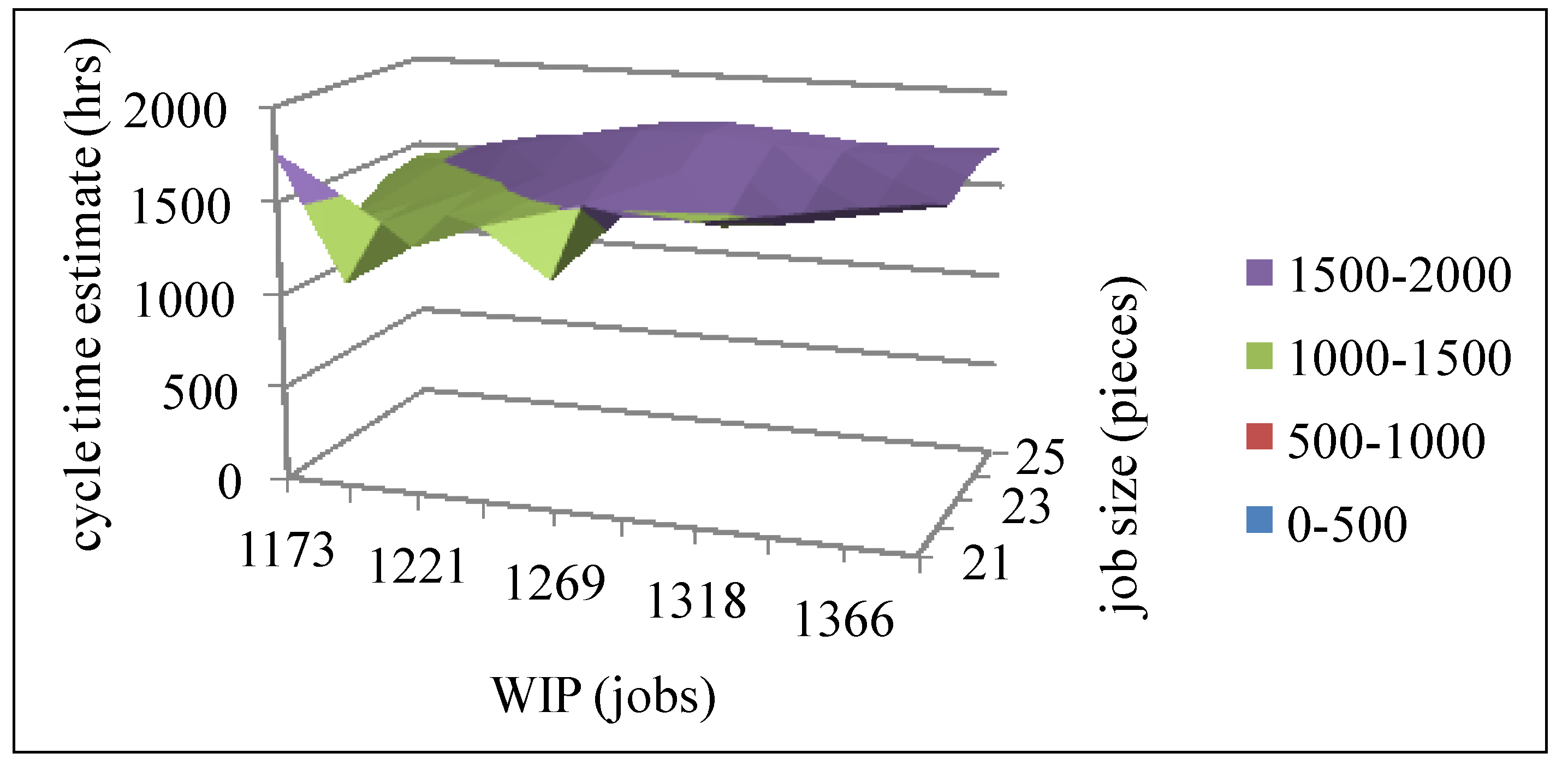
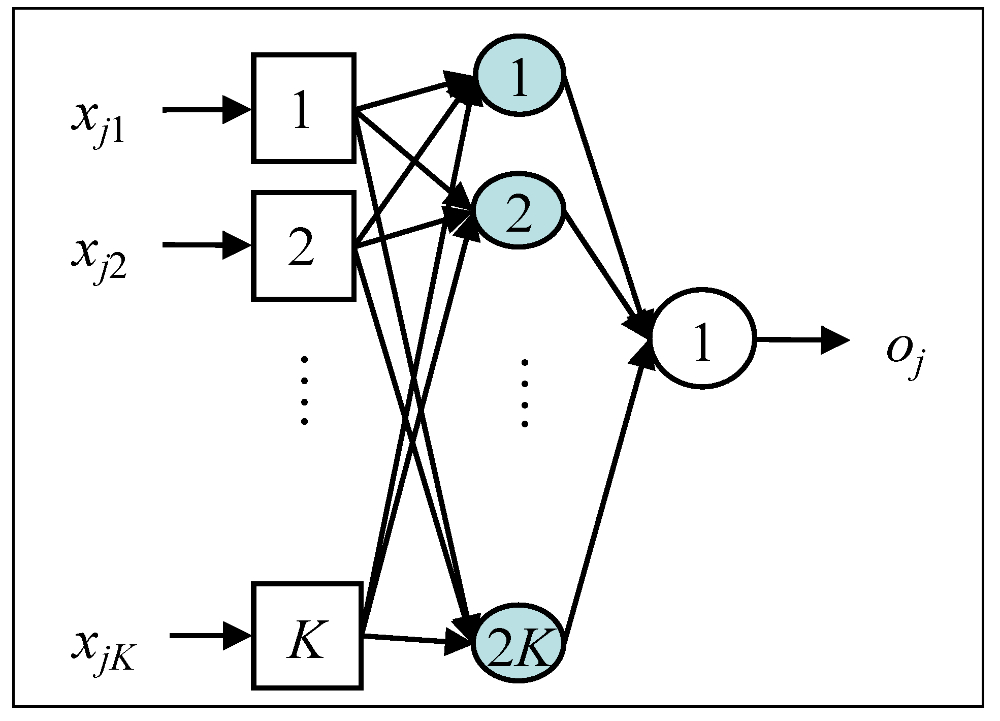
Subsequently, the values of the six controllable variables were normalized to 0.1–0.9 (see Table 6). Then, a BPN was established to fit the relationship between the job cycle time and the six controllable variables. The BPN has a single hidden layer with 12 nodes, and was trained with 3/4 of the collected data using the gradient descent algorithm. The remaining 1/4 were reserved for evaluating the performance of the BPN. BPN training stopped if the MSE was less than 10⁻⁵ or 15000 epochs have been run. To visualize the relationship, it was projected down to the three-dimensional space, as shown in Figure 4

Table 6. The normalized values of the six controllable variables.

j	xj1	xj2	xj3	xj4	xj5	xj6	aj
1	0.700	0.284	0.200	0.811	0.202	0.337	0.186
2	0.500	0.292	0.350	0.237	0.283	0.738	0.432
3	0.900	0.318	0.100	0.452	0.717	0.495	0.475
4	0.500	0.502	0.375	0.835	0.294	0.667	0.205
5	0.300	0.760	0.800	0.621	0.748	0.674	0.383
116	0.500	0.649	0.100	0.233	0.170	0.670	0.693
117	0.300	0.539	0.150	0.803	0.409	0.190	0.426
118	0.500	0.100	0.175	0.746	0.224	0.181	0.108
119	0.700	0.458	0.625	0.330	0.087	0.592	0.348
120	0.300	0.638	0.225	0.690	0.629	0.513	0.463

Table 6. The normalized values of the six controllable variables.

j	xj1	xj2	xj3	xj4	xj5	xj6	aj
1	0.700	0.284	0.200	0.811	0.202	0.337	0.186
2	0.500	0.292	0.350	0.237	0.283	0.738	0.432
3	0.900	0.318	0.100	0.452	0.717	0.495	0.475
4	0.500	0.502	0.375	0.835	0.294	0.667	0.205
5	0.300	0.760	0.800	0.621	0.748	0.674	0.383
116	0.500	0.649	0.100	0.233	0.170	0.670	0.693
117	0.300	0.539	0.150	0.803	0.409	0.190	0.426
118	0.500	0.100	0.175	0.746	0.224	0.181	0.108
119	0.700	0.458	0.625	0.330	0.087	0.592	0.348
120	0.300	0.638	0.225	0.690	0.629	0.513	0.463

Figure 4. The relationship projected down to the three-dimensional space.

Figure 4. The relationship projected down to the three-dimensional space.

Finally, the BPN can be used to estimate the cycle time with any setting of the six controllable variables.

3.1. Example 1

If the job size = 25 pieces, factory WIP = 1246 jobs, the queue length before the bottleneck = 170 jobs, the queue length on the route = 726 jobs, the average waiting time = 243 h, and factory utilization = 89%, then the estimated cycle time is 1665 h.

In addition, we can assess the effectiveness of a cycle time reduction action.

3.2. Example 2

In the previous example, if factory WIP, the queue length before the bottleneck, and the queue length on the route can all be reduced by 5%, i.e.,

• factory WIP = 1183 jobs;
• the queue length before the bottleneck = 161 jobs;
• the queue length on the route = 690 jobs;
• then the estimated cycle time can be shortened from 1665 hours to 1586 hours, with a reduction of 4.75%.
• Further, it is also possible to develop an action to achieve the cycle time improvement target.

3.3. Example 3

In the previous example, if the cycle time is to be improved by 7%, by lowering the WIP level in the factory, then the factory WIP should be reduced from 1246 jobs to 1208 jobs, which is equal to a percentage of 3.1%.

There are a number of possible actions that may achieve the cycle time reduction target. For example, in the previous example, five such actions are listed in Table 7. However, not all of them are feasible, or even effective. To assess the feasibility of each action, the mean absolute percentage deviation between the target values and the historical values, MAPD_h, has to be less than a threshold θ₁ that was set to 4%. The assessment results were summarized in Table 8. Among the five actions, only three of them were feasible. Subsequently, the most effective cycle time reduction action is the feasible one that minimizes the mean absolute percentage deviation between the target values and the original values of the controllable variables, i.e., MAPD_o. The results are shown in Table 9. Obviously, the most effective action is action #2 in this example. Subsequently, the conclusion was handed over to a production control engineer to be confirmed. The confirmation results were shown in Table 10. The expert believed that the proposed action was basically feasible.

The financial benefits of the cycle time reduction action can be described by the following analysis. The factory releases about 30,000 pieces of wafers per month. The unit cost of each finished wafer is about $17000. Therefore, the opportunity cost of a wafer in progress can be approximated as 17000/2 = 8500 dollars per day, assuming it is half-finished. A reduction of 7% in the cycle time is about five days. In total, the annual savings of the opportunity costs by the cycle time reduction action is about 8500 × 30,000 × 12 × 5 = 15.3 billion dollars. As capital adequacy is very important for a semiconductor manufacturer, we believe such benefits can improve the sustainable development of the semiconductor manufacturer.

Table 7. Five possible actions to achieve a cycle time reduction of 7%.

Action #	Content	Estimated Cycle time Reduction
1	Reduce factory WIP by 3.1%	7%
2	Reduce the job size by 8%	7%
	Reduce factory WIP by 1%
	Reduce the queue length before the bottleneck by 3%
	Reduce the queue length on the route by 3%
	Reduce the average waiting time by 3%
3	Reduce the job size by 4%	7%
	Reduce the queue length before the bottleneck by 8%
	Reduce the average waiting time by 31%
	Reduce factory utilization by 8%
4	Reduce the job size by 4%%	7%
	Reduce factory WIP by 4%
	Reduce the queue length before the bottleneck by 4%
	Reduce the queue length on the route by 9%,
	Reduce the average waiting time by 59%
	Reduce factory utilization by 3%
5	Reduce the job size by 8%	7%
	Increase factory WIP by 2%
	Reduce the queue length before the bottleneck by 4%
	Reduce the queue length on the route by 6%
	Reduce the average waiting time by 14%
	Reduce factory utilization by 1%

Table 7. Five possible actions to achieve a cycle time reduction of 7%.

Action #	Content	Estimated Cycle time Reduction
1	Reduce factory WIP by 3.1%	7%
2	Reduce the job size by 8%	7%
	Reduce factory WIP by 1%
	Reduce the queue length before the bottleneck by 3%
	Reduce the queue length on the route by 3%
	Reduce the average waiting time by 3%
3	Reduce the job size by 4%	7%
	Reduce the queue length before the bottleneck by 8%
	Reduce the average waiting time by 31%
	Reduce factory utilization by 8%
4	Reduce the job size by 4%%	7%
	Reduce factory WIP by 4%
	Reduce the queue length before the bottleneck by 4%
	Reduce the queue length on the route by 9%,
	Reduce the average waiting time by 59%
	Reduce factory utilization by 3%
5	Reduce the job size by 8%	7%
	Increase factory WIP by 2%
	Reduce the queue length before the bottleneck by 4%
	Reduce the queue length on the route by 6%
	Reduce the average waiting time by 14%
	Reduce factory utilization by 1%

Table 8. The feasibility assessment results.

Action #	MAPDh	Feasibility
1	4.2%	Infeasible
2	2.5%	Feasible
3	3.7%	Feasible
4	4.1%	Infeasible
5	2.7%	Feasible

Table 8. The feasibility assessment results.

Action #	MAPDh	Feasibility
1	4.2%	Infeasible
2	2.5%	Feasible
3	3.7%	Feasible
4	4.1%	Infeasible
5	2.7%	Feasible

Table 9. The effectiveness evaluation results.

Action #	MAPDo	Effectiveness
2	3.1%	Most effective
3	8.6%	-
5	5.8%	-

Table 9. The effectiveness evaluation results.

Action #	MAPDo	Effectiveness
2	3.1%	Most effective
3	8.6%	-
5	5.8%	-

Table 10. The confirmation results.

Action	Confirmation Result
Reduce the queue length before the bottleneck by 3%	It can be taken, but will it lead to a reduction in the factory monthly output?
Reduce the queue length on the route by 3%	It can be taken by controlling the inputs to the route.
Reduce the average waiting time by 3%	It is a good direction, but unsure how to take.

Table 10. The confirmation results.

Action	Confirmation Result
Reduce the queue length before the bottleneck by 3%	It can be taken, but will it lead to a reduction in the factory monthly output?
Reduce the queue length on the route by 3%	It can be taken by controlling the inputs to the route.
Reduce the average waiting time by 3%	It is a good direction, but unsure how to take.

4. Conclusions and Future Research Directions

Enhancing the competitiveness and sustainability has been pursued by every semiconductor manufacturer. A key to this is the production cycle time. Shortening the production cycle time improves the responsiveness to customer demands, and leads to significant profits from yield improvement and cost reduction. However, in the past, cycle time reduction is usually unplanned owing to the lack of a systematic and quantitative procedure. To tackle this problem, a systematic procedure was established in this study for planning cycle time reduction actions to enhance the competitiveness and sustainability of a semiconductor manufacturer. First, some controllable factors that are influential to the job cycle time are identified. Subsequently, the relationship between the controllable factors and the job cycle time is fitted with a BPN. Based on this relationship, actions to shorten the job cycle time can be planned. The feasibility and effectiveness of an action have to be assessed before it is taken in the practice.

An example containing the real data of hundreds of jobs has been used to illustrate the applicability of the proposed methodology. The results showed that the proposed methodology is indeed an easy-to-use and efficient procedure. It guided the planning of cycle time reduction step by step, and was also able to list a number of possible solutions to choose from. That provides much flexibility in practice. Further, from the financial analysis, the value of the cycle time reduction action to the sustainable development of the semiconductor manufacturer is even more obvious, since semiconductor manufacturing is a burning-money industry. However, any conclusion from the proposed procedure has to be confirmed by the production control engineer.