Sources of China’s Economic Growth: An Empirical Analysis Based on the BML Index with Green Growth Accounting

Abstract

This study develops a biennial Malmquist–Luenberger productivity index that is used to measure the sources of economic growth by utilizing data envelopment analysis and the directional distance function. Taking restrictions on resources and the environment into account based on the green growth accounting framework; we split economic growth into seven components: technical efficiency change, technological change, labor effect, capital effect, energy effect, output structure effect and environmental regulation effect. Further, we apply the Silverman test and Li-Fan-Ullah nonparametric test in combination with kernel distribution to test for the counterfactual contributions at the provincial level in China from 1998 to 2012. The empirical results show that: (1) technological progress and TFP make positive contributions to economic growth in China, while technical efficiency drags it down; (2) the effect of output structure and CO₂ emissions with environmental regulation restrain economic growth in some provinces; and (3) overall, physical capital accumulation is the most important driving force for economic take-off, irrespective of whether the government adopts environmental regulations.

1. Introduction

Over the past 30 years, economic growth in China has attracted worldwide attention since the country embarked on reform and opened up. However, China has paid a heavy price in terms of resources and the environment for its significant economic growth. After the Asian economic crisis in 1997, some scholars even began to question whether China’s overheating economic growth is sustainable. Krugman [1] argued that Asia, including China, succeeded because of its investment in resources instead of a promotion of efficiency. During the period of the “11th five-year plan”, China’s resource productivity was at $320–$350 per tonnes with the rapid growth of direct material input, and the output efficiency of its resources was below those of developed countries. Its CO₂ emissions were generated by primary energy doubled from 3.47 to 7.18 billion tonnes from 2000 to 2009, making China a major contributor of CO₂ emissions in the world. By the end of 2006, however, China had made some substantial progress in pollution reduction. The economic benefits arising from the implementation of its cleaner production program amounted to 4.4 billion CNY, and the direct economic benefits generated by energy saving amounted to 5.5 billion CNY. However, the costs of environmental pollution abatement are still increasing along with economic development. In 2011, the country’s environmental pollution control investment was 602.62 billion CNY, accounting for 1.27% of GDP. Consequently, the high intensity of resource consumption and environmental pollution shows that Chinese economic growth is still mainly based on the extensive growth feature of high input, high consumption, high emission and growth without development, and is not driven by the green growth approach of improving TFP.

Suffering from the dual challenge of economic growth and resource and environmental constraints, China must implement strict or appropriate environmental regulation, energy savings initiatives and other mechanisms to reduce the negative impact on its environment without reducing the rate of economic growth. Further, China urgently needs to transform the pattern of economic growth so as to realize a win-win solution for environmental protection and economic growth. To this end, it is necessary to understand what the sources of the country’s economic growth are. However, the traditional accounting of sources of economic growth does not consider the factors of energy and the environment. In addition, this accounting method may lead to a misleading result.

Thus, the main purpose of this study is to discover China’s sources of economic growth with the constraints of resources and the environment. The study uses the frontier technology boundary analysis and output-oriented directional distance function (DDF) to propose a decomposition of the sources of economic growth within the green growth accounting framework (GGAF), and then to measure the sources of China’s economic growth between 1998 and 2012 based on the new biennial Malmquist–Luenberger productivity index.

The rest of this paper is organized as follows. The next section features a brief review of the relevant literature pertaining to the sources of economic growth. The theoretical methods, which contain the biennial Malmquist–Luenberger productivity index and the GGAF, are introduced in Section 3. Section 4 discusses the data and empirical results. In Section 5 describes the above tests that were conducted to further analyze the distribution dynamics of economic growth from 1998 to 2012. Finally, Section 6 presents the conclusions and policy implications derived from the study.

2. Literature Review

Economic growth is an important foundation for the economic and social development of a country or region. Thus, its sources, internal mechanisms, and implementation have become core issues that economists continue to explore. Much of the existing literature has described and analyzed the sources of China’s economic growth. Some researchers [2,3,4] showed that China’s economic growth mainly comes from factor accumulation, especially capital. Chow [5] first discovered that capital accumulation played a major role in explaining China’s growth from 1952 to 1980 with the absence of technical progress. Kim and Lau [6] applied the aggregate meta-production function framework and found that growth mostly resulted from the growth of tangible inputs, that is, capital and labor, and not technical progress or TFP. Other researchers later found that TFP was the primary driving force behind China’s growth [7,8,9,10]. Borensztein and Ostry [11] believed China’s technological progress was slow even though TFP made a remarkable contribution in the post-reform period. Hu and Khan [12] further found that the sharp and sustained increase in TFP accounted for the unprecedented economic growth observed during the reform period while capital accumulation played an important role in China’s economic growth from 1952 to 1994. Chow and Li [13] found that productivity growth accounted for almost 32% of growth, while capital accounted for 54% and labor 13%. However, Ding and Knight [14] concluded that structural change and productive efficiency, benefiting from the improved resource allocation, technology and competition, helped to explain the remarkably high growth rate.

An assessment of the above literature indicates that previous studies have two shortcomings. On one hand, most studies used the parametric method, but this method’s accounting accuracy in terms of economic growth has been questioned [15,16] because it needs to set the production function and the error term. On the other hand, the studies focused on traditional factors, but not on energy consumption and CO₂ emissions with environmental regulation. Energy and the environment are endogenous variables and double rigid constraints on economic growth. The dual reversed transmission mechanism of the influence of energy conservation and environmental regulation on economic growth, can promote energy productivity and the transformation of the pattern of economic development. Energy consumption is a forceful driver for the growth of GDP [17,18,19,20]. Koop [21] noted that input changes of CO₂ emissions are a negligible factor in explaining growth. Chang [22] concluded that GDP growth is indissociable from increases in both energy consumption and CO₂ emissions. Wang et al. [23] found that reducing CO₂ emissions may handicap China’s economic growth to some degree. Kareem et al. [24] found a causal relationship between CO₂ emissions and economic growth with the causality running from CO₂ emissions to economic growth. However, most of the researchers investigated the existence and direction of Granger causality between economic growth, energy, and CO₂ emissions, rather than growth accounting incorporating energy and environmental regulation.

If the composition of output and the methods of production are immutable, then the environment would be inextricably linked to the scale of global economic activity [25]. CO₂ emissions, a measure of environmental regulation variables, can be chosen as an input [26,27] or an output by using the DDF with the nonparametric method such as data envelopment analysis (DEA) [28,29,30,31]. This nonparametric method does not set the form of production functions and especially can be used for growth accounting with multiple inputs and outputs. Therefore, to contribute to the existing literature, this study first expands the biennial Malmquist productivity index proposed by Pastor et al. [32] and constructs a biennial Malmquist–Luenberger productivity index with the biennial environmental DEA technology, which can avoid infeasibilities and measures technological progress and regress. Second, this study adds energy and environmental factors into the decomposition and proposes a GGAF emphasizing energy saving and environmental protection. The change in economic growth can be decomposed into seven components: technical efficiency change, technological change, and the effects of labor, capital, energy, output structure, and CO₂ emissions with environmental regulation. Finally, this study utilizes the Silverman test to test for multimodality and the nonparametric Li-Fan-Ullah test to analyze the distribution dynamics of economic growth between actual and counterfactual distributions.

3. Method

3.1. Environmental Production Technology

In order to take resources and the environment into account, we decompose change in economic growth by using the environmental production technology that produces desirable outputs jointly with undesirable outputs. For each time period t = 1,2,...,T, the environmental production technology is described by the output set S(t) that can be jointly produced from the input vector (L, K, E) as follows:

(1)

where the variables L,K,E Є R₊ denote an input vector for labor, capital and energy, respectively; Y Є R₊ denotes the desirable or good output of gross regional product (GRP); and C Є R₊ represents undesirable or bad output of CO₂ emissions.

The output set S(t) is assumed to satisfy the standard properties of a technology, that is, S(t) is compact for each input and is a closed set; and inputs and the desirable output are strong or freely disposable. In order to formulate S(t) as an environmental technology, we need to impose two additional environmental axioms: the null-jointness or by-product axiom; and the weak disposability of joint outputs axiom. The first axiom indicates that if firms do not produce a good output, then it is not possible to produce bad output. The second axiom indicates that if all inputs (L, K, E) can produce outputs (Y, C), then it is feasible to reduce these outputs proportionally by θ where (Y’, C’) = (θY, θC) and 0 ≤ θ ≤ 1. This axiom reveals that it is costly to dispose of an undesirable output with the environmental regulated technology. In other words, we can construct the output set that satisfies the above properties and axioms as

(2)

where i = 1, 2, ..., I denotes observations of inputs and outputs; z_i is the weight assigned to each observation when constructing the production possibilities frontier; and z_i > 0 means that the production technology exhibits constant returns-to-scale (CRS). In addition, the output set at the time period t + 1 can be similarly defined as S(t + 1).

Based on the technologies at time periods t and t + 1, Pastor et al. [32] introduced a new technology called the biennial technology. The biennial technology can be defined as the convex hull of the period t and t + 1 technologies. Taking the undesirable output into account, we can obtain the biennial environmental technology, which can be denoted as

S(B) = conv{S(t), S(t + 1)}

(3)

3.2. Biennial Malmquist–Luenberger Index

The traditional production function does not reflect the effect of changes in desirable and undesirable outputs in the production process. In accordance with the shortage function [33], Chambers et al. [34] constructed the DDF, which measures the distance to the observation from the production boundary. The output-oriented DDF, which is an alternative representation of the above technology, measures the distance from an observation to the production frontier. The directional output distance function provides a good method for modeling economic and environmental performances. This function at time period t with the biennial technology is defined as

(4)

where g = (g_y, − g_c) is a direction vector, and measures the maximum proportional expansion of both desirable and undesirable outputs (Y^t, C^t), given the input vector (L^t, K^t, E^t) and the biennial technology in the direction g. Following [32], we introduce a TFP index called the biennial Malmquist–Luenberger index (hereafter, BML index). Taking the biennial production technology as a reference, the BML index between period t and t + 1 is given by

(5)

Equation (5) shows that the BML index is decomposed into two components: technical efficiency change, or EFF and technological change, or TC. The first component, EFF, which indicates a catching-up effect, measures the change in the distance towards the best practice frontier from time period t to t + 1. The second component, TC, which measures technological progress or regress, captures the degree to which the production function shifts from period t to t + 1 by taking the biennial technology as a reference. Because the biennial technology is defined as the convex hull of the period t and t + 1 technologies, we do not need to take the arithmetic mean or geometric mean when defining the BML index.

3.3. Green Growth Accounting Framework

The traditional economic growth accounting method only accounts for and analyses the traditional production factors (such as labor and capital). In contrast, the modern economic growth accounting method not only considers the effect of traditional factors, but also focuses on energy and environmental factors that can affect economic growth. Under the restrictions of resource and environment, combined with the DDF and the BML index, we measure the sources of economic growth by utilizing the GGAF method.

Using biennial CRS technology, we can decompose the change in economic growth between time periods t and t + 1 as per the following equation: where Y^t, Y^t+1 represent the actual desirable output at times t and t + 1 respectively; the functions F^t (L^t, K^t, E^t, Y^t, C^t, g) and F^t+1 (L^t+1, K^t+1, E^t+1, Y^t+1, C^t+1, g) represent the maximum potential desirable output at times t and t +1 given input, desirable output and technology, respectively; and similarly, the functions F^B (L^t, K^t, E^t, Y^t, C^t, g) and F^B (L^t+1, K^t+1, E^t+1, Y^t+1, C^t+1, g) represent the maximum potential desirable output given the biennial technology at times t and t + 1, respectively.

(6)

(7)

Equation (6) shows that economic growth change can be decomposed into three components: maximum potential economic growth change (PEGCH), which is measured by using the biennial technology as a reference; technical efficiency change (EFF); and technological change (TC). The first term, PEGCH, measures the maximum potential economic growth change depending on the changes in L, K, E, Y and C along the current period’s production frontier. When we assume that the reference technology exhibits CRS, it follows that we can further separate PEGCH into five components by isolating the effects of changes in L, K, E, Y and C between the two time periods with the biennial technology.

Combining Equations (6) and (7), the complete seven-factor decomposition of economic growth with the GGAF method can be obtained by:

Y^t+1/Y^t = EFF × TC × LE × KE × EE × CAE × OSE = TFP × IME × OME

(8)

The decomposition result from Equation (8) suggests that economic growth with environment regulation is affected by these seven factors. The last five components, measure the effects on economic growth of changes in labor (LE), capital (KE), energy (EE), CO₂ emissions (CAE) and output structure (OSE) with environmental regulation, respectively. The product of LE, KE and EE is the change in the input mix effect (IME). Similarly, the product of the last two effects is the change in the output mix effect (OME).

It is noted that the decomposition of change in economic growth in Equation (8) considers the restrictions of energy and environment. Traditional economic growth accounting does not take energy and the environment into account; its inputs only include labor and capital stock, and its output is GRP, not CO₂ emissions. Because one output, GRP, is considered, the effect of the change in output structure is equal to 1 and we can ignore it in the decomposition. Thus, according to the above-mentioned accounting idea, the decomposition of economic growth in the traditional model without environment regulation is given by:

Y^t+1/Y^t = EFF × TC × LE × KE = TFP × IME

(9)

According to the application of a DEA-type linear programming approach, we can use this method to calculate the value of the seven components and then solve the following LP problem:

(10)

4. Data and Empirical Results

4.1. Data

This study considers 30 provinces in China as research subjects. Data for 15 years between 1998 and 2012 are collected for the empirical analysis. The variables include the inputs (labor, capital stock and energy consumption), and outputs (GRP and CO₂ emissions) in each region. As we aim to study the effects of resources and the environment on economic growth, especially the effect of CO₂ emissions on economic growth, we select energy consumption as one of inputs and CO₂ emissions as one of outputs [35,36]. CO₂, an environmental factor, is an undesirable by-product accompanied by the production. In addition, CO₂ is mainly due to the use of energy (especially fossil energy), so we should take energy into account.

The data on labor input and GRP are obtained directly from the China Statistical Yearbook [37]. Labor input is measured by the number of employees. Data for total energy consumption are collected from the China Energy Statistical Yearbook [38]. Energy consumption consists of coal, washing coal, coke, oven gas, oil, gasoline, diesel, fuel, kerosene, liquefied petroleum, natural gas, refinery gas and others. The physical quantity of all energy is converted to a standard amount. There are no official data available for the capital stock of Chinese provinces. Following the perpetual inventory method, the capital stock for each province in year t is calculated as [39]:

(11)

where K₁₉₀₀ is the initial value of the capital stock in 1900, I is the real value of gross fixed capital formation, and δ is the depreciation rate. To estimate the capital stock, we need to determine the initial capital stock and depreciation rate. We assume that the initial capital stock in 1900 is 0. This assumption is based on the fact that the capital stock from 1900 to 1952 was completely depreciated. Using investment data from 1952 to 2012 obtained in all provinces, we perform regressions between the logarithmic of the existing investment data and time series data. In addition, then we simulate the 1900 to 1951 sequence investment data for all provinces. Following a recent study by [40], we adopt different depreciation rates for each province.

The actual provincial CO₂ emissions cannot be obtained directly from the official data. CO₂ emissions mainly result from fossil energy consumption. The publication Guidelines for National Greenhouse Gas Inventories [41] provides a reference formula to estimate CO₂ emissions. Following this method, we can use provincial-level energy consumption to forecast CO₂ emissions in each province. The forecasting equation is given by:

(12)

where j represents the type of energy; E represents a variety of energy consumption; and NCV, CEF and COF represent the average low calorific values of energy, carbon emission coefficients and the carbon oxidation factor, respectively.

Table 1 shows the summary statistics of all variables. All nominal variables are deflated to real variables by using a price index for the year 2000. The mean value of desirable output GRP is 6620.05 (100 million CNY), whereas the undesirable output of CO₂ is 23,104.14 (10000 tonnes). In addition, those of labor, capital stock and energy consumption are 2304.33 (10000 persons), 18,642.29 (100 million CNY), 8797.01 (10000 tonnes), respectively. From these values, we can know that China is a big country in terms of energy consumption and CO₂ emissions. Clearly, the high growth in China shows obvious features of high investment, high energy consumption and high emissions. Therefore, the study of China’s economic growth can no longer ignore the source of energy and environmental elements.

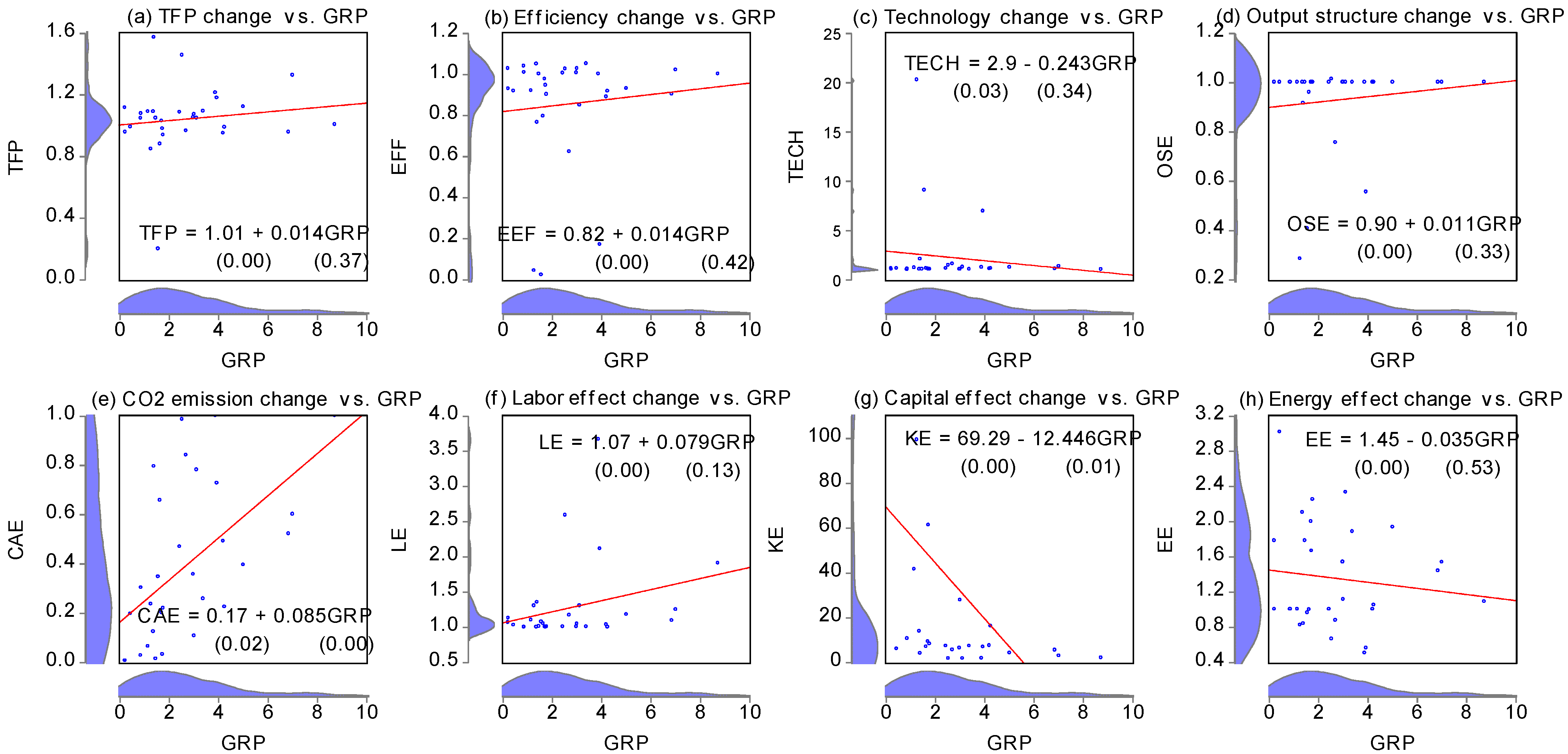
4.2. Empirical Results

According to our GGAF method, we can estimate economic growth and its sources at the provincial level. Table 2 shows each of the components of the decomposition of economic growth from 1998 to 2012 [42]. The first row of Columns 2 to 9 for each province reports the contributions to changes in economic growth from the effects of the changes in TFP, technical efficiency, technology, labor and capital stock without environment regulation. The second row for each province with environment regulation shows the contributions to changes in economic growth from the effects of changes in output structure, CO₂ emissions, and energy consumption, including five other components.

Table 1. Summary statistics of input and output variables, 1998–2012.

Variables	Mean	S.D.	Max	Min
Gross regional product (100 million CNY)	6,620.05	6,671.37	42,860.33	223.88
Carbon dioxide emissions (10000 tonnes)	23,104.14	18,408.14	106,667.02	892.85
Labor (10000 persons)	2,304.33	1,525.40	6,288.00	230.40
Capital stock (100 million CNY)	18,642.29	17,905.59	110,064.98	953.54
Energy consumption (10000 tonnes)	8,797.01	6,970.46	40,630.76	384.48

Table 1. Summary statistics of input and output variables, 1998–2012.

Variables	Mean	S.D.	Max	Min
Gross regional product (100 million CNY)	6,620.05	6,671.37	42,860.33	223.88
Carbon dioxide emissions (10000 tonnes)	23,104.14	18,408.14	106,667.02	892.85
Labor (10000 persons)	2,304.33	1,525.40	6,288.00	230.40
Capital stock (100 million CNY)	18,642.29	17,905.59	110,064.98	953.54
Energy consumption (10000 tonnes)	8,797.01	6,970.46	40,630.76	384.48

Table 2. Decomposition indexes of Economic growth between 1998 and 2012.

Provinces	TFP	EFF	TC	OSE	CAE	LE	KE	EE
Beijing	1.004	0.983	1.022			1.018	1.087
	1.031	1.002	1.029	1.002	0.998	1.079	1.037	0.964
Tianjin	1.034	1.014	1.019			1.015	1.090
	1.044	0.991	1.053	0.994	0.978	1.037	1.106	0.983
Hebei	0.982	0.986	0.995			1.005	1.126
	0.997	0.991	1.006	1.000	0.939	1.005	1.180	1.000
Shanxi	0.972	0.977	0.995			1.004	1.143
	0.891	0.760	1.172	0.938	0.916	1.007	1.452	0.997
Inner Mongolia	0.995	0.990	1.004			1.006	1.155
	0.979	0.751	1.303	0.899	0.879	1.022	1.485	0.986
Liaoning	1.029	0.997	1.032			1.009	1.076
	1.006	0.864	1.164	0.953	0.975	1.059	1.177	0.959
Jilin	0.988	0.986	1.002			1.005	1.130
	0.993	0.983	1.010	0.997	0.951	1.005	1.186	1.000
Heilongjiang	1.007	1.011	0.996			1.005	1.094
	0.978	0.939	1.042	0.976	0.980	1.018	1.175	0.990
Shanghai	1.018	1.000	1.018			1.032	1.056
	1.014	1.000	1.014	0.999	1.001	1.110	1.041	0.947
Jiangsu	1.036	1.005	1.031			1.008	1.076
	1.023	1.000	1.022	1.000	0.961	1.016	1.089	1.034
Zhejiang	1.023	0.993	1.030			1.014	1.076
	1.010	0.994	1.016	1.000	0.921	1.012	1.130	1.049
Anhui	0.980	1.000	0.980			1.000	1.139
	1.006	0.999	1.007	1.000	0.938	1.000	1.182	1.000
Fujian	1.013	0.997	1.016			1.012	1.091
	1.005	0.987	1.018	1.000	0.975	1.020	1.049	1.067
Jiangxi	0.969	0.989	0.980			1.000	1.152
	1.005	0.999	1.006	1.000	0.871	1.000	1.210	1.054
Shandong	0.999	0.995	1.004			1.005	1.119
	0.999	0.993	1.007	1.000	0.953	1.006	1.142	1.026
Henan	0.959	0.974	0.984			1	1.164
	1.004	0.996	1.007	1.000	0.865	1.000	1.287	0.998
Hubei	0.980	0.996	0.984			1.004	1.135
	1.006	1.001	1.005	1.000	0.833	1.004	1.316	1.008
Hunan	0.973	0.993	0.980			1.000	1.145
	1.006	1.000	1.006	1.000	0.910	1.000	1.175	1.036
Guangdong	1.001	1.000	1.001			1.018	1.099
	1.000	1.000	1.000	1.000	1.000	1.053	1.060	1.003
Guangxi	0.946	0.965	0.981			0.999	1.181
	0.993	0.988	1.005	1.000	0.865	1.000	1.214	1.071
Hainan	1.032	1.003	1.029			1.015	1.059
	0.997	0.989	1.008	1.000	0.858	1.002	1.182	1.095
Chongqing	0.974	0.994	0.980			1.000	1.154
	1.009	1.004	1.005	1.000	0.837	1.000	1.254	1.061
Sichuan	0.981	1.001	0.980			1.000	1.141
	1.010	1.005	1.005	1.000	0.893	1.000	1.180	1.051
Guizhou	0.981	1.002	0.980			1.000	1.133
	1.004	1.002	1.002	1.000	0.743	1.000	1.490	1.000
Yunnan	0.971	0.991	0.980			1.000	1.137
	1.000	0.995	1.004	1.000	0.741	1.000	1.433	1.040
Shaanxi	1.004	1.008	0.996			1.002	1.119
	1.003	0.998	1.005	1.000	0.704	1.002	1.527	1.042
Gansu	0.974	0.994	0.980			1.000	1.140
	1.006	1.000	1.006	1.000	0.896	1.000	1.231	1.000
Qinghai	1.029	1.000	1.030			1.010	1.075
	1.008	0.998	1.009	1.000	0.649	1.006	1.618	1.051
Ningxia	1.018	0.995	1.023			1.010	1.085
	0.996	0.993	1.003	1.000	0.651	1.010	1.704	1.000
Xinjiang	1.020	0.992	1.028			1.011	1.069
	1.004	0.991	1.014	1.000	0.801	1.011	1.355	1.000
Weighted Mean	0.996	0.994	1.002			1.007	1.115
	1.001	0.974	1.032	0.992	0.883	1.016	1.256	1.017

Table 2. Decomposition indexes of Economic growth between 1998 and 2012.

Provinces	TFP	EFF	TC	OSE	CAE	LE	KE	EE
Beijing	1.004	0.983	1.022			1.018	1.087
	1.031	1.002	1.029	1.002	0.998	1.079	1.037	0.964
Tianjin	1.034	1.014	1.019			1.015	1.090
	1.044	0.991	1.053	0.994	0.978	1.037	1.106	0.983
Hebei	0.982	0.986	0.995			1.005	1.126
	0.997	0.991	1.006	1.000	0.939	1.005	1.180	1.000
Shanxi	0.972	0.977	0.995			1.004	1.143
	0.891	0.760	1.172	0.938	0.916	1.007	1.452	0.997
Inner Mongolia	0.995	0.990	1.004			1.006	1.155
	0.979	0.751	1.303	0.899	0.879	1.022	1.485	0.986
Liaoning	1.029	0.997	1.032			1.009	1.076
	1.006	0.864	1.164	0.953	0.975	1.059	1.177	0.959
Jilin	0.988	0.986	1.002			1.005	1.130
	0.993	0.983	1.010	0.997	0.951	1.005	1.186	1.000
Heilongjiang	1.007	1.011	0.996			1.005	1.094
	0.978	0.939	1.042	0.976	0.980	1.018	1.175	0.990
Shanghai	1.018	1.000	1.018			1.032	1.056
	1.014	1.000	1.014	0.999	1.001	1.110	1.041	0.947
Jiangsu	1.036	1.005	1.031			1.008	1.076
	1.023	1.000	1.022	1.000	0.961	1.016	1.089	1.034
Zhejiang	1.023	0.993	1.030			1.014	1.076
	1.010	0.994	1.016	1.000	0.921	1.012	1.130	1.049
Anhui	0.980	1.000	0.980			1.000	1.139
	1.006	0.999	1.007	1.000	0.938	1.000	1.182	1.000
Fujian	1.013	0.997	1.016			1.012	1.091
	1.005	0.987	1.018	1.000	0.975	1.020	1.049	1.067
Jiangxi	0.969	0.989	0.980			1.000	1.152
	1.005	0.999	1.006	1.000	0.871	1.000	1.210	1.054
Shandong	0.999	0.995	1.004			1.005	1.119
	0.999	0.993	1.007	1.000	0.953	1.006	1.142	1.026
Henan	0.959	0.974	0.984			1	1.164
	1.004	0.996	1.007	1.000	0.865	1.000	1.287	0.998
Hubei	0.980	0.996	0.984			1.004	1.135
	1.006	1.001	1.005	1.000	0.833	1.004	1.316	1.008
Hunan	0.973	0.993	0.980			1.000	1.145
	1.006	1.000	1.006	1.000	0.910	1.000	1.175	1.036
Guangdong	1.001	1.000	1.001			1.018	1.099
	1.000	1.000	1.000	1.000	1.000	1.053	1.060	1.003
Guangxi	0.946	0.965	0.981			0.999	1.181
	0.993	0.988	1.005	1.000	0.865	1.000	1.214	1.071
Hainan	1.032	1.003	1.029			1.015	1.059
	0.997	0.989	1.008	1.000	0.858	1.002	1.182	1.095
Chongqing	0.974	0.994	0.980			1.000	1.154
	1.009	1.004	1.005	1.000	0.837	1.000	1.254	1.061
Sichuan	0.981	1.001	0.980			1.000	1.141
	1.010	1.005	1.005	1.000	0.893	1.000	1.180	1.051
Guizhou	0.981	1.002	0.980			1.000	1.133
	1.004	1.002	1.002	1.000	0.743	1.000	1.490	1.000
Yunnan	0.971	0.991	0.980			1.000	1.137
	1.000	0.995	1.004	1.000	0.741	1.000	1.433	1.040
Shaanxi	1.004	1.008	0.996			1.002	1.119
	1.003	0.998	1.005	1.000	0.704	1.002	1.527	1.042
Gansu	0.974	0.994	0.980			1.000	1.140
	1.006	1.000	1.006	1.000	0.896	1.000	1.231	1.000
Qinghai	1.029	1.000	1.030			1.010	1.075
	1.008	0.998	1.009	1.000	0.649	1.006	1.618	1.051
Ningxia	1.018	0.995	1.023			1.010	1.085
	0.996	0.993	1.003	1.000	0.651	1.010	1.704	1.000
Xinjiang	1.020	0.992	1.028			1.011	1.069
	1.004	0.991	1.014	1.000	0.801	1.011	1.355	1.000
Weighted Mean	0.996	0.994	1.002			1.007	1.115
	1.001	0.974	1.032	0.992	0.883	1.016	1.256	1.017

If the government does not implement green policies, such as environmental controls, firms would not need to pay for pollution emissions from their production process and thus would have little incentive to innovate and improve clean production technologies. Evidently, the differences in the means of changes in TFP, technical efficiency and technology are not substantially altered by environmental regulation. The effects of technical efficiency change on economic growth are less than 1 on average, implying a negative contribution of technical efficiency to economic growth. The biggest efficiency improvements taking measures of environmental governance appear in developed regions, such as Beijing, Chongqing, Guangdong and Jiangsu, as well as in backward areas, such as Guizhou and Sichuan. The mean score of technological change increases from 1.002 to 1.032 with the incorporation of environmental regulation. This indicates that environmental regulation is conducive to regional enterprises adopting new technologies and promotes technological progress. Among them, the provinces demonstrating rapid technological progress are Beijing, Tianjin, Fujian, Inner Mongolia, Liaoning, and Shanxi. We specifically need to point out that some provinces, including Beijing, Inner Mongolia, Liaoning, Shanxi, and Tianjin, emerge with technological progress greater than 1, considering energy and environmental factors. With environmental regulation, TFP did not appear to deteriorate in the case of the deterioration of technical efficiency. The great improvement in TFP (from 0.996 to 1.001 on average) is driven primarily by the rapid increase in technological progress. The TFP indices are generally higher in developed regions such as Beijing, Guangdong, Jiangsu, Shanghai, Tianjin, Liaoning, Heilongjiang and Zhejiang. This study demonstrates that technological progress and TFP make positive contributions to economic growth in China, while technical efficiency drags it down.

As shown in Columns 5 to 6 in Table 2, the accounting results of the changes in output structure and CO₂ emissions are less than 1 on average, considering environmental regulation. These results indicate that the exacerbation of output structure and CO₂ emissions effects have an adverse impact on economic growth and inhibit the growth of GRP in the long run. The output structure effect in most provinces is not less than 1 and promotes economic growth. Compared with Beijing, Chongqing, Gansu and other provinces, Tianjin, Heilongjiang, Inner Mongolia, Liaoning and Shanxi exhibit the smallest output structure effects, which are 0.994, 0.976, 0.899, 0.953 and 0.938, respectively. In terms of the CO₂ emissions effect, 28 provinces have scores far smaller than 1, while rich regions such as Shanghai and Guangdong exhibit values equal to one. In fact, if there is no cycle of production technology and other advanced conditions, the more CO₂ emissions, the more inputs such as raw materials are needed in the production process, which causes enterprises to produce less desirable outputs. Thus, the regulation of CO₂ emissions could restrain GDP growth to some extent.

The last three columns of Table 2 report the effects of the input mix. As is shown, the accumulation of physical capital plays a decisive role in economic growth. The effect of physical capital rose to 1.256 with environmental regulation from 1.115 without environmental regulation. LE exhibited no significant change. It is interesting to note that the KE of 26 provinces greatly improved after the consideration of environmental regulation, while that of Beijing, Fujian, Guangdong and Shanghai declined, albeit their LE greatly improved. With regard to the energy effect, EE on average made some contribution to economic growth. Over the 15-year period, the energy effect had a greater impact on economic growth in Jiangsu, Shandong, Hainan, Chongqing, Fujian, Guangxi, Hunan, Qinghai, Sichuan and Zhejiang. EE was equal to 1 in Anhui, Jilin, Gansu, Guizhou, Hebei, Ningxia and Xinjiang, but EE exerted a negative influence on economic growth in eight provinces, including Beijing, Heilongjiang, and Shanghai.

To demonstrate the relationship between the contributing factors and the initial level of GRP, Figure 1 plots the decomposition indexes against GRP in 1998, along with GLS regression lines [43,44,45]. Figure 1a shows that TFP change was positively correlated to GRP in 1998. Figure 1b shows a similar relationship between technical efficiency change and GRP. Both regression slope coefficients were statistically insignificant, demonstrating that neither TFP change nor technical efficiency change contributed significantly to economic convergence at the provincial level in China from 1998 to 2010. The statistically significant negative slope coefficient in Figure 1c suggests that the effect of technological change significantly contributed to convergence in economic growth. The positive sign of the statistically insignificant slope coefficients in Figure 1d–f indicate that the effects of changes in output structure, CO₂ emissions and labor did not significantly contribute to convergence, even though the contribution of CO₂ emissions had a wide dispersion. Figure 1g shows that the regression coefficient for change in physical capital accumulation was negative and statistically significant, indicating that the change contributed to convergence. Finally, as shown in Figure 1h, even if the contribution of the energy effect showed a wide dispersion and its coefficient was negative, the coefficient was statistically insignificant, suggesting that the energy effect also contributed little to convergence.

Figure 1. Decomposition components plotted against GRP in 1998.

Figure 1. Decomposition components plotted against GRP in 1998.

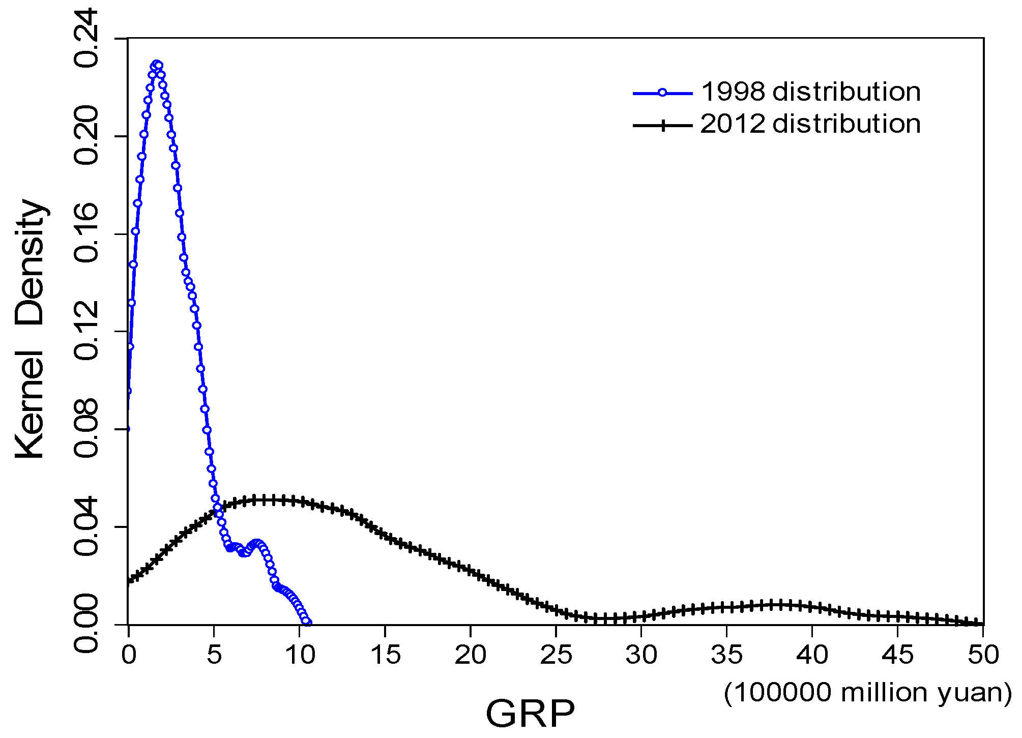
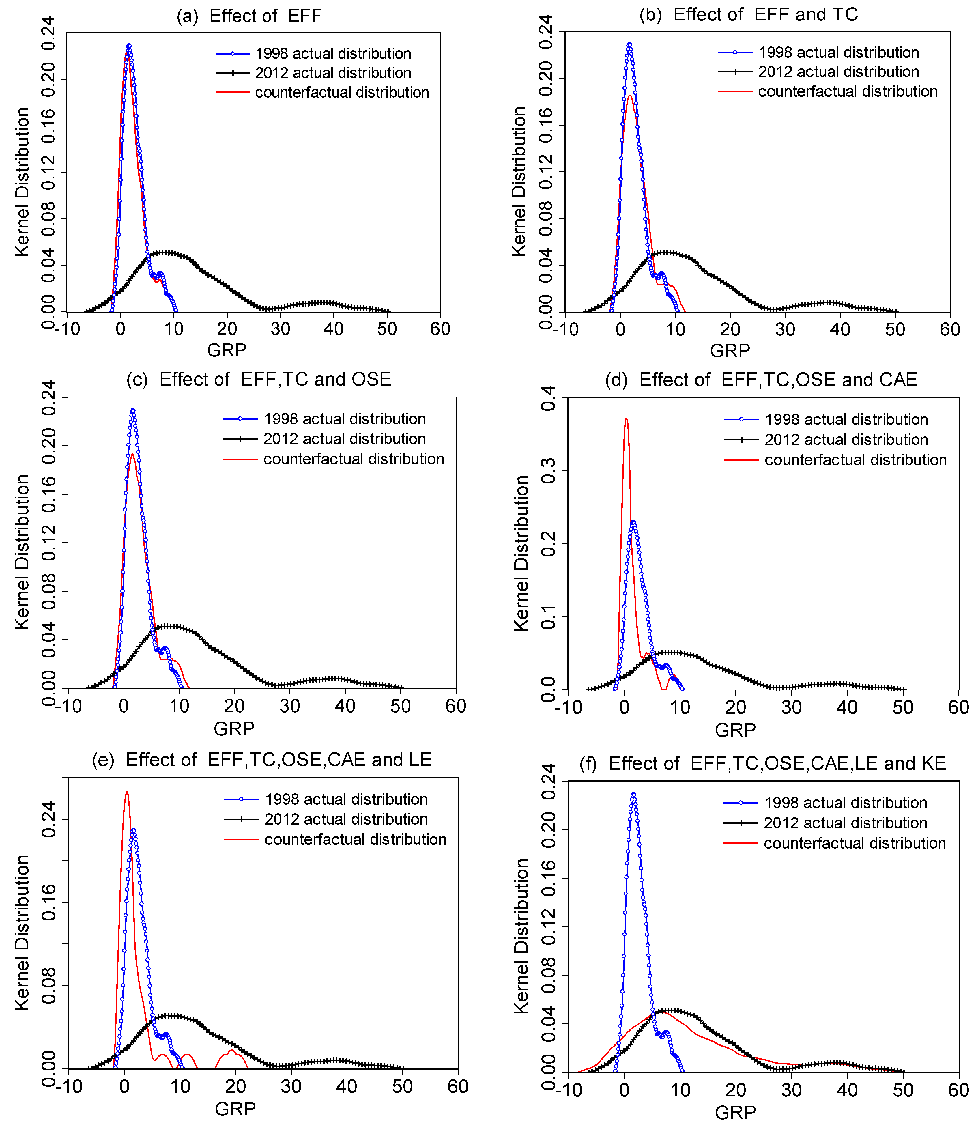
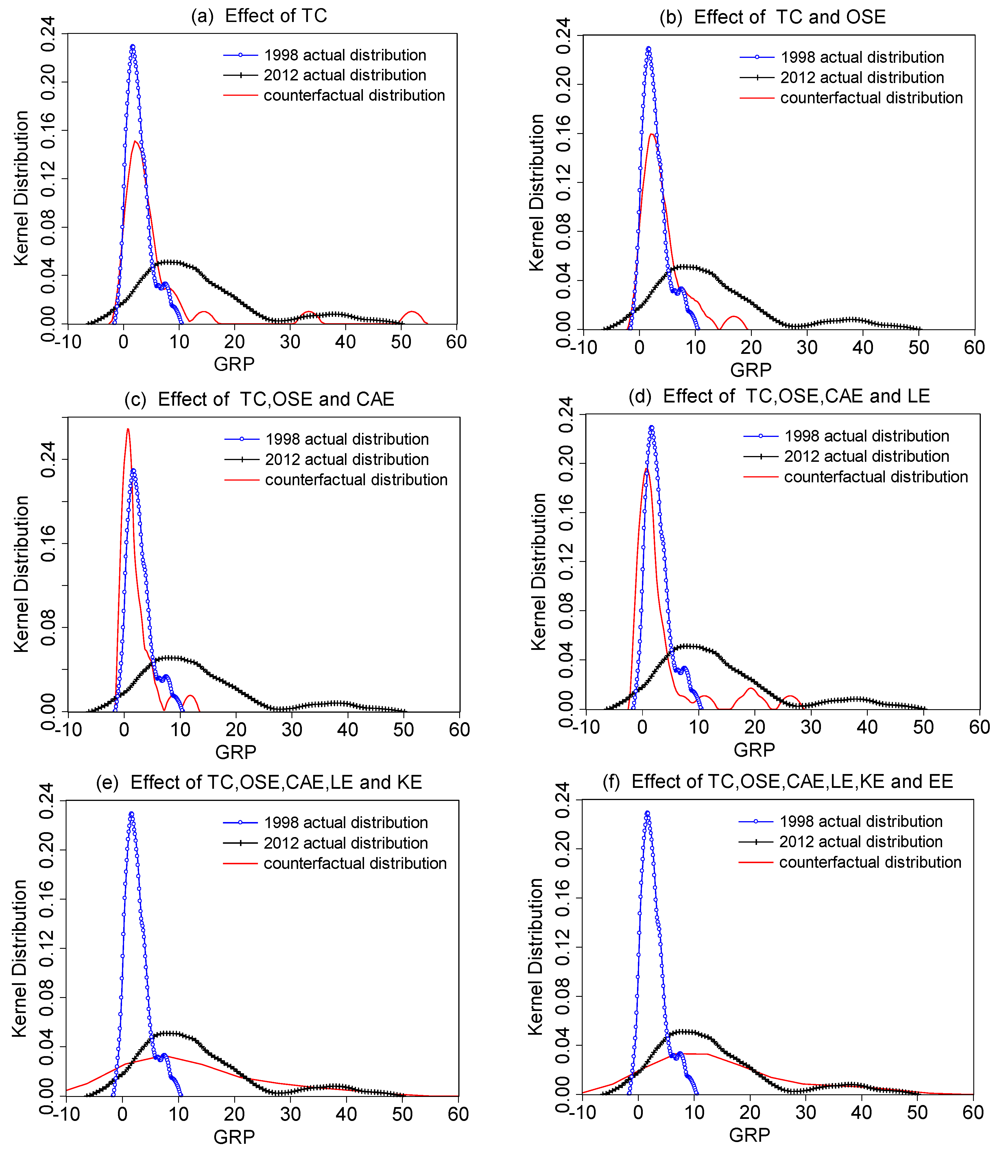
5. Analysis of Distributions Dynamics of Economic Growth

Although we now understand the relationship between the contributing factors and the initial level of GRP, we should further analyze the distribution dynamics of economic growth from 1998 to 2012. Figure 2 describes the plots of the distributions of GRP across 30 provinces in 1998 and 2012. It is easy to determine that the distribution of GRP in 1998 is unimodal, but after 15 years, this distribution appears to bimodal with a higher mean in 2012.

Figure 2. Actual distributions of GRP in 1998 and 2012.

Figure 2. Actual distributions of GRP in 1998 and 2012.

Silverman [46] proposed a method (called the Silverman test) to test for the transformation theoretically [47,48]. With the application of this test for the multimodality of the actual distributions in 1998 and 2012, Table 3 reports the statistical significance levels for the tests of the null hypothesis that the kernel density has at most j modes against the alternative that it has more than j modes. As shown in Table 3, the p-value in the 1998 distribution is 0.262 with the null hypothesis that the kernel density has one mode, indicating that the 1998 distribution has a single mode. For the 2012 distribution, the null hypothesis that it has one mode is rejected (the p-value is 0.043) while the null hypothesis that it has two modes cannot be rejected (the p-value is 0.523). This shows that the 2012 distribution is indeed bimodal. Thus, it is true that the distributions of economic growth moved from being unimodal to bimodal over the 15-year period.

Table 3. Silverman test for multimodality of the actual distributions.

Distributions	p-values
	H0: One Mode H1: More than One Mode	H0: Two Modes H1: More than Two Modes
Y98	0.262 (H0 not reject)	0.323 (H0 not reject)
Y12	0.043 (H0 reject)	0.523 (H0 not reject)

Note: Y⁹⁸, Y¹² denote GRP across provinces in 1998 and 2012, respectively.

Table 3. Silverman test for multimodality of the actual distributions.

Distributions	p-values
	H0: One Mode H1: More than One Mode	H0: Two Modes H1: More than Two Modes
Y98	0.262 (H0 not reject)	0.323 (H0 not reject)
Y12	0.043 (H0 reject)	0.523 (H0 not reject)

Note: Y⁹⁸, Y¹² denote GRP across provinces in 1998 and 2012, respectively.

To further enhance this result of multimodality and understand the degree to which each of the seven components of the decomposition of economic growth change affect the distribution of economic growth from 1998 to 2012, we extend the analysis of the distribution dynamics by using the actual and counterfactual method with a nonparametric test, as developed by [49] and [50]. The method tests for the statistical significance of the differences between actual and counterfactual distributions that are two unknown distributions. Wang [51] also employed this test to study economics. The method indirectly tests for the statistical significance between the relative counterfactual distributions of the seven components of the decomposition of economic growth and the actual 2012 distribution. If we set the two unknown distributions as f and g, then the null hypothesis of this test is H₀: f(x) = g(x) for all x, and the alternative is H₁: f(x) ≠ g(x) for some x. The decomposition of economic growth change with environment regulation in Equation (8) can be re-expressed as:

Y¹² = (EFF × TC × LE × KE × EE × CAE × OSE) × Y⁹⁸

(13)

Therefore, GRP across the provinces in 2012 can be constructed by successively multiplying GRP in 1998 by each of the seven components. According to this idea, we can segregate the effect on the counterfactual distribution dynamics of economic growth by the sequential introduction of each of these components. If we consider only the impact of change in technical efficiency, the counterfactual GRP distribution of the variable in 2012 can be given by

(14)

If we multiply by the effect on technological change once more on the right side of Equation (14), the counterfactual GRP distribution of the variable in 2012 can be given by

(15)

Analogously, we can obtain the remaining counterfactual GRP distributions of the variables generated by sequential introduction of components of the decomposition. Ultimately, these results test for the counterfactual distributions and the actual 2012 distribution as shown in Appendix Table A1.

As Appendix Table A1 shows, the first t-test statistic value is 3.0925, which rejects the null hypothesis at the 1% significance level. This test result is consistent with Figure 2 and the result of the Silverman test in Table 3, suggesting that the counterfactual distribution is significantly different to the actual 1998 distribution. The next seven tests demonstrate the null hypothesis of identity of the counterfactual distributions by the sequential introduction of the seven contributing components of change in economic growth and the actual 2012 distribution. At the 1% significance level, Test 7 with physical capital accumulation alone easily accepts the null hypothesis and the other tests reject the null hypothesis that the counterfactual distributions are not identical to the actual 2012 distribution. These seven results indicate that physical capital accumulation is the key force for transforming the economic growth distribution and this factor alone made a big contribution to the shift to bimodality from 1998 to 2012. The other six factors played a minor role in explaining the comprehensive change in the distribution between 1998 and 2012. Tests 9 to 127 compare the actual distribution in 2012 with the counterfactual distribution with effects from the given two, three, four, five and six of the seven components.

The above analysis on economic growth distribution dynamics uses a formal test for the statistical significance of the differences between the counterfactual distributions and the actual distribution in 2012. Simultaneously, these results can be reinforced and illustrated by using figures of kernel distribution as shown in Figure 3 to Figure 4. Figure 3a, which is only combined with the effect of technical efficiency change, shows that the counterfactual distribution seems to be identical to the actual 1998 distribution, not the actual 2012 distribution. This indicates that technical efficiency made a small contribution to the promotion of convergence of the distribution. Even though the counterfactual distribution includes the effects from the changes in technology, output structure, CO₂ emissions and labor successively in Figure 3b–e, these results would not change dramatically. Until it takes physical capital accumulation into account, there is almost no significant difference between the counterfactual and the 2012 distributions (see Figure 3f). The results in Figure 3a–f are consistent with Test 2, 9, 30, 65, 100 and 121 in Appendix Table A1.

Figure 4a compares the actual 1988 and 2012 distributions with the counterfactual 2012 distribution, combined only with technological change. It shows that the kurtosis of the counterfactual 2012 distribution reduces, but is still different to the actual 2012 distribution. When combined with output structure change in Figure 4b, the shape of these distributions does not change much. These results indicate that both the effect of technological change and the joint effect of technological change and output structure change played a minor role in economic growth over the 1998 to 2012 period. Considering the additional effect from the changes in CO₂ emissions and labor in Figure 4c,d, the counterfactual distribution moves much closer to the actual 1998 distribution. When physical capital accumulation is added to the counterfactual distribution in Figure 4e, its mode shifts to the left and it moves much closer to the actual 2012 distribution. This demonstrates that physical capital accumulation is the core contributor to change in economic growth. Figure 4f describes the counterfactual distribution with the joint effect of six components including the change in energy consumption. It illustrates that the counterfactual distribution moves further toward the actual 2012 distribution, though its shape changes only slightly and its tail extends. In addition, the six panels of Figure 4 can be reinforced by the nonparametric test corresponding to Tests 3, 15, 45, 85, 115 and 127 in Appendix Table A1.

Figure 3. Counterfactual and actual distributions of economic growth with the effect of technical efficiency change (EFF).

Figure 3. Counterfactual and actual distributions of economic growth with the effect of technical efficiency change (EFF).

According to the analysis, we can successively introduce the changes in output structure, CO₂ emissions, labor, physical capital accumulation and energy consumption in combination with each other. However, regardless of whether the combinations include two, three, four, five or six components of the decomposition, the shape of the counterfactual distribution does not change significantly. Only when physical capital accumulation is added to these combinations does the counterfactual distribution increasingly exhibit a bimodal shape and appear identical to the actual 2012 distribution. In summary, along with the process of economic growth, physical capital accumulation plays the most important role in changing the distribution from unimodal to bimodal during the period of 1998–2012.

Figure 4. Counterfactual and actual distributions of economic growth with the effect of TC.

Figure 4. Counterfactual and actual distributions of economic growth with the effect of TC.

6. Conclusions

In this paper, we introduce a new biennial Malmquist–Luenberger productivity index by using the biennial environmental DEA technology and directional distance function. Based on the proposed BML index in consideration of resources and the environment, this article employs the green growth accounting framework to decompose economic growth change into seven components at the Chinese provincial level during the period from 1998 to 2012. These decompositions can measure the impact of the changes in technical efficiency, technology, output structure, CO₂ emissions, labor, physical capital accumulation and energy consumption on economic growth.

The results demonstrate that TFP promotes rapid economic growth, mainly because technology has made great progress, and even compensates for the negative effect brought about by the deterioration of efficiency, and technological progress contributes to convergence. However, the improvement of output structure is not apparent. The effect of CO₂ emissions with the emergence of a serious deterioration discouraged economic growth in some provinces between 1998 and 2012. Labor and energy are important sources of economic growth and their increase stimulates rapid economic growth. The energy effect contributed little to convergence. Undoubtedly, a high physical capital accumulation is the most important driving force for economic take-off, irrespective of whether the government implements environmental regulation or not, and it also makes a big contribution to convergence. In other words, economic growth is still mainly dependent on factor inputs, but not efficiency or TFP in China.

After that, we apply the Silverman test to confirm that the economic distribution changes from unimodal in 1998 to bimodal with a higher mean in 2012. In addition, the nonparametric test, in combination with some figures of kernel distribution, is performed to clarify the effect of each component of the decomposition on economic growth and makes the results more robust. Therefore, based on our research findings, the Chinese government needs to recognize that the high growth in factor inputs will not only result in a waste of resources, but also in environmental pollution. In order to achieve resource-saving, environmentally-friendly and sustainable macroeconomic growth, China should increase public investment in education and technology, accelerate industrial upgrading and then enhance the rate of technological progress and TFP. Only in this way can Chinese economic growth transform from an extensive program of increasing factor inputs to one with a green growth pattern driven by TFP.

The method of the green growth accounting framework can decompose economic growth change into seven components, and estimate the degree to which each of the seven components of the decomposition of economic growth change affect the distribution of economic growth from 1998 to 2012. However, there is sampling variability and thus statistical uncertainty about these estimates [30]. Parteka and Wolszczak-Derlacz [52] followed a bootstrap procedure to obtain bias-corrected estimates of Malmquist indices and their components and their confidence intervals [53]. Therefore, we can further adopt consistent bootstrap estimation procedures to obtain bias-corrected estimates of these indices and their confidence intervals, which test the significance of these indices’ effects on economic growth.

References and Notes

1. Krugman, P. The myth of Asia’s miracle. Foreign Aff. 1994, 73, 62–78. [Google Scholar]
2. Han, G.F.; Kalirajan, K.; Singh, N. Productivity and economic growth in East Asia: Innovation, efficiency and accumulation. Jpn. World Econ. 2002, 14, 401–424. [Google Scholar]
3. Wang, Y.; Yao, Y.D. Sources of China’s economic growth 1952–1999: Incorporating human capital accumulation. China Econ. Rev. 2003, 14, 32–52. [Google Scholar]
4. Zhao, C.W.; Du, J. Capital formation and economic growth in western China. Chin. Econ. 2009, 42, 7–26. [Google Scholar] [CrossRef]
5. Chow, G.C. Capital formation and economic growth in China. Q. J. Econ. 1993, 108, 809–842. [Google Scholar] [CrossRef]
6. Kim, J.I.; Lau, L.J. The sources of economic growth of the East Asian newly industrialized countries. J. Jpn. Int. Econ. 1994, 8, 235–271. [Google Scholar] [CrossRef]
7. Young, A. Gold into base metals: Productivity growth in the People’s Republic of China during the reform period. J. Polit. Econ. 2003, 111, 1220–1261. [Google Scholar] [CrossRef]
8. Arayama, Y.; Miyoshi, K. Regional diversity and sources of economic growth in China. World Econ. 2004, 27, 1583–1607. [Google Scholar] [CrossRef]
9. Islam, N.; Dai, E.; Sakamoto, H. Role of TFP in China’s growth. Asian Econ. J. 2006, 20, 127–159. [Google Scholar]
10. Jefferson, G.H.; Hu, A.G.Z.; Su, J. The sources and sustainability of China’s economic growth. Brook. Pap. Econ. Act. 2006, 2, 1–47. [Google Scholar] [CrossRef]
11. Borensztein, E.; Ostry, D.J. Accounting for China’s growth performance. Am. Econ. Rev. 1996, 86, 224–228. [Google Scholar]
12. Hu, Z.F.; Khan, M.S. Why is China growing so fast? Staff. Pap. Int. Monet. Fund 1997, 44, 103–131. [Google Scholar] [CrossRef]
13. Chow, G.C.; Li, K.W. China’s economic growth: 1952–2010. Econ. Dev. Cult. Chang. 2002, 51, 247–256. [Google Scholar] [CrossRef]
14. Ding, S.; Knight, J. Why has China grown so fast? The role of structural change. Available online: http://www.economics.ox.ac.uk/materials/working_papers/paper415.pdf (access on 1 September 2014).
15. Nadiri, M.I.; PruchaI, R. Dynamic Factor Demand Models and Productivity Analysis. In New Developments in Productivity Analysis; Hulten, C.R., Dean, E.R., Harper, M., Eds.; University of Chicago Press: Chicago, IL, USA, 2001. [Google Scholar]
16. Gong, B.; Sickles, R. Finite sample evidence on the performance of stochastic frontiers and data envelopment analysis using panel data. J. Econ. 1992, 51, 259–284. [Google Scholar]
17. Shiu, A.; Lam, P.L. Electricity consumption and economic growth in China. Energy Policy 2004, 32, 47–54. [Google Scholar] [CrossRef]
18. Zhou, G.; Chau, K.W. Short and long-run effects between oil consumption and economic growth in China. Energy Policy 2006, 34, 3644–3655. [Google Scholar] [CrossRef]
19. Yuan, J.H.; Kang, J.G.; Zhao, C.H.; Hu, Z.G. Energy consumption and economic growth: Evidence from China at both aggregated and disaggregated levels. Energy Econ. 2008, 30, 3077–3094. [Google Scholar] [CrossRef]
20. Yalta, A.T.; Cakar, H. Energy consumption and economic growth in China: A reconciliation. Energy Policy 2012, 41, 666–675. [Google Scholar] [CrossRef]
21. Koop, G. Carbon dioxide emissions and economic growth: A structural approach. J. Appl. Stat. 1998, 25, 489–515. [Google Scholar] [CrossRef]
22. Chang, C.C. A multivariate causality test of carbon dioxide emissions, energy consumption and economic growth in China. Appl. Energy 2010, 87, 3533–3537. [Google Scholar] [CrossRef]
23. Wang, S.S.; Zhou, D.Q.; Zhou, P.; Wang, Q.W. CO2 emissions, energy consumption and economic growth in China: A panel data analysis. Energy Policy 2011, 39, 4870–4875. [Google Scholar] [CrossRef]
24. Kareem, S.D.; Kari, F.; Alam, G.M.; Adewale, A.; Oke, O.K. Energy consumption, pollutant emissions and economic growth: China experience. Int. J. Appl. Econ. Financ. 2012, 6, 136–147. [Google Scholar] [CrossRef]
25. Grossman, G.M.; Krueger, A.B. Economic growth and the environment. Q. J. Econ. 1995, 110, 353–377. [Google Scholar] [CrossRef]
26. Hailu, A.; Veeman, T.S. Environmentally sensitive productivity analysis of the Canadian pulp and paper industry, 1959–1994: An input distance function approach. J. Environ. Econ. Manag. 2000, 40, 251–274. [Google Scholar] [CrossRef]
27. Coelli, T.; Lauwers, L.G.; Huylenbroeck, V. Formulation of Technical, Economic and Environmental Efficiency Measures that are Consistent with the Materials Balance Condition; CEPA Working Paper Series, No WP062005. The University of Queensland: Brisbane, Australia, 2005. Available online: http://www.uq.edu.au/economics/cepa/docs/WP/WP062005.pdf (access on 1 September 2014).
28. Chung, Y.H.; Färe, R.; Grosskopf, S. Productivity and undesirable outputs: A directional distance function approach. J. Environ. Manag. 1997, 51, 229–240. [Google Scholar] [CrossRef]
29. Fare, R.; Grosskopf, S.; Margaritis, D. APEC and the Asian economic crisis: Early signals from productivity trends. Asian Econ. J. 2001, 15, 325–342. [Google Scholar] [CrossRef]
30. Jeon, B.M.; Sickles, R.C. The role of environmental factors in growth accounting. J. Appl. Econ. 2004, 19, 567–591. [Google Scholar] [CrossRef]
31. Kumar, S. Environmentally sensitive productivity growth: A global analysis using Malmquist–Luenberger index. Ecol. Econ. 2006, 56, 280–293. [Google Scholar] [CrossRef]
32. Pastor, J.T.; Asmild, M.; Lovell, C.A. The biennial Malmquist productivity change index. Soc. Econ. Plan. Sci. 2011, 45, 10–15. [Google Scholar] [CrossRef]
33. Luenberger, D.G. New optimality principles for economic efficiency and equilibrium. J. Optim. Theory Appl. 1992, 75, 221–264. [Google Scholar] [CrossRef]
34. Chambers, R.G.; Chung, Y.; Färe, R. Benefit and distance functions. J. Econ. Theory 1996, 70, 407–419. [Google Scholar] [CrossRef]
35. Wei, C.; Ni, J.; Du, L. Regional allocation of carbon dioxide abatement in China. China Econ. Rev. 2012, 23, 552–565. [Google Scholar] [CrossRef]
36. Choi, Y.; Zhang, N.; Zhou, P. Efficiency and abatement costs of energy-related CO2 emissions in China: A Slacks-based Efficiency Measure. Appl. Energy 2012, 98, 198–208. [Google Scholar] [CrossRef]
37. National Bureau of Statistics. China Statistical Yearbook; China Statistical Press: Beijing, China, 2011. [Google Scholar]
38. Department of Industry and Transport Statistics; National Bureau of Statistics (NBS); Energy Bureau; National Development and Reform Commission (NDRC) (Eds.) China Energy Statistical Yearbook; China Statistical Press: Beijing, China, 2011. (in Chinese)
39. Wu, Y. Openness, productivity and growth in the APEC economies. Empir. Econ. 2004, 29, 593–604. [Google Scholar] [CrossRef]
40. Wu, Y. China’s contribution to productivity growth: New estimates. China Econ. Q. 2008, 3, 827–842. [Google Scholar]
41. Eggleston, H.S.; Buendia, L.; Miwa, K.; Ngara, T.; Tanabe, K. IPCC Guidelines for National Greenhouse Gas Inventories in 2006; IGES: Kanagawa, Japan, 2006. [Google Scholar]
42. These values are on weighted mean by GRP proportion of each province mean between 1998 and 2012.
43. Kumar, S.; Russell, R.R. Technological change, technological catch-up, and capital deepening: Relative contributions to growth and convergence. Am. Econ. Rev. 2002, 92, 527–548. [Google Scholar] [CrossRef]
44. Henderson, J.D.; Russell, R.R. Human capital and convergence: A production-frontier approach. Int. Econ. Rev. 2005, 46, 1167–1205. [Google Scholar] [CrossRef]
45. Kumar and Russell and Henderson and Russell use the same regression to describe labor productivity and its components growth rates. We also employ generalized least squares because the error term is likely to be heteroskedastic. These results are consistent with White test of OLS.
46. Silverman, B.W. Using kernel density estimates to investigate multimodality. J. R. Stat. Soc. 1981, 43, 97–99. [Google Scholar]
47. Bianchi, M. Testing for convergence: Evidence from non-Parametric multimodality tests. J. Appl. Econ. 1997, 12, 393–409. [Google Scholar] [CrossRef]
48. The proposed test was first applied to an OECD economic research by Bianchi, M.
49. Li, Q. Nonparametric testing of closeness between two unknown distribution functions. Econ. Rev. 1996, 15, 261–274. [Google Scholar] [CrossRef]
50. Fan, Y.; Ullah, A. On goodness-of-fit tests for weekly dependent processes using kernel method. J. Nonparametric Stat. 1999, 11, 337–360. [Google Scholar] [CrossRef]
51. Wang, C.H. Sources of energy productivity growth and its distribution dynamics in China. Resour. Energy Econ. 2011, 33, 279–292. [Google Scholar] [CrossRef]
52. Parteka, A.; Wolszczak-Derlacz, J. Dynamics of productivity in higher education: Cross-european evidence based on bootstrapped Malmquist indices. J. Product. Anal. 2013, 40, 67–82. [Google Scholar] [CrossRef]
53. Simar, L.; Wilson, P. Estimating and bootstrapping Malmquist indices. Eur. J. Oper. Res. 1999, 115, 459–471. [Google Scholar] [CrossRef]