Spatio-Temporal Characteristics of Rural Economic Development in Eastern Coastal China

Abstract

Although the regional differences of rural economic development can be easily determined, a challenging problem for research studies regarding rural economic development has been the inter-relatedness between different areas, and this challenge has been noted remarkably little in research data to date. As an empirical investigation, this study analyzes the spatio-temporal characteristics of rural economic development from a period beginning in 1978 to the year 2012, in the eastern coastal region of China. In order to determine the special differentiation characteristics of rural economic development, three indexes, namely the Gini coefficient (G), Tsui–Wang index (TW) and Theil index (T), were employed. To explore the inter-relatedness among the different areas, we selected a spatial autocorrelation model. The results indicated that, to a large extent, rural economic development from 1978 to 2012 in the eastern coastal region of China was greatly influenced, and the per capita annual net income changed significantly, due to the process of rapid urbanization and industrialization. Generally speaking, the annual net income constantly increased, from 87.7 USD in 1978 to 1628.1 USD in 2012. However, the calculation results indicated that the per capita income gap in the same province decreased, while the gap between the provinces presented an aggregate trend. The regional polarization widened continuously. It was also found that the spatial positive autocorrelation for the regional economy was significant, with a waving and ascending trend, and the neighbor effect of regional economic growth was continuously strengthened. Qualitative analysis of the driving mechanism was applied, and it was determined that there are three primary factors affecting the development of the rural regions, namely resource endowments, economic location and policies.

1. Introduction

Rural economic development is arguably one of the most important themes in rural areas. There are four major elements of rural development, which are economic, social, cultural-human and environment [1,2]. In fact, the economic level of specific counties is also a factor for determining the degree of rural area development. For example, the economy is still considered the backbone of the rural regions. Furthermore, rural development plays a vital role in urban development, as well as regional economic growth [3]. Therefore, rural development has become a significant research area, which focuses on promoting thinking, practices and developing tools and ideas in this field, in order to foster the types of rural economic development opportunities that many countries are committed to expanding.

Insight into the driving factors behind the economic performance of rural regions is both of scientific interest and high political relevance [4,5]. Despite the existence of a well-established body of research data regarding differential economic performance, specific research into this issue in rural areas only truly began in the late 1980s and early 1990s [1]. The perception of rural development has undergone considerable changes in the past 30 years, and it has become a multi-dimensional issue [2]. Academicians have paid a great deal of attention to the importance of natural resources, environmental dimensions of rural development and economic dimensions [6,7,8,9,10]. Meanwhile, a growing number of studies have found that the economic development level in those rural areas, especially in districts close to cities with highly liberalized economies [11], is higher than that of remote rural areas.

Questions still remain regarding whether location has an effect on rural economic development and if the neighborhood effect exists in rural economic development. In actuality, studies regarding the effects of location on economic development, as well as the neighborhood effect in economic development have garnered extensive attention from research groups [12,13]. However, these research studies from the perspective of rural economic development remain scarce and require improvement.

Environmental quality and natural heritage vary geographically to an extent, as does the amount of rural economic development opportunities [7,14]. There is a close connection between income and the economic development and regional resources. In fact, the national income per capita has been used as the most popular factor for measuring development. It has been found that rural economic development can vary over time and by location [2]. In the same rural district, the economic development is constantly changing. It is uniformly found that different places are experiencing different phrases at the same time. It is thus easy to raise questions, such as what are the variances of the often-posed questions in the economic literature regarding the driving forces and why economic growth rates differ among countries or regions [4]. One often asked question is whether or not they connect with each other. Indeed, rural economic development explores many characteristics, such as dynamic variability, diversity, relativity, etc. However, despite the fact that rural research is very pluralistic, both in terms of its study themes and target areas [15], those characteristics and driving mechanisms have not yet received a great deal of attention in the current research.

With the aim of constructing an analytical model for rural economic development, the eastern coastal regions of China have been adopted as the case study areas. By way of selecting the assessment indices and models, the spatial and temporal disparities, along with the agglomeration characteristics in rural economic development were reviewed. Finally, based on these characteristics, the mechanisms driving rural economic development were investigated, such as the effects of regional location on regional rural economic development. The study results provide scientific references regarding the development of related policies for rural economic development.

2. Materials and Methodology

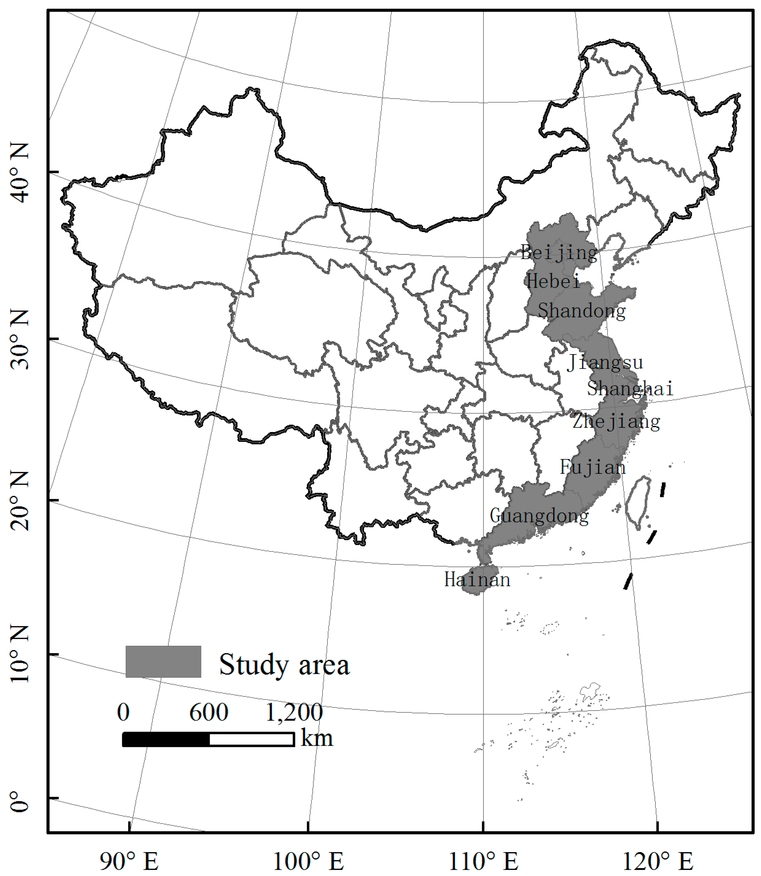
2.1. Study Area and Data

The current study area covered ten provinces and municipalities, which lie in the eastern coastal region of China. They are Hebei (HB), Beijing (BJ), Tianjin (TJ), Shandong (SD), Jiangsu (JS), Shanghai (SH), Zhejiang (ZJ), Fujian (FJ), Guangdong (GD) and Hainan (HN), located from the north to the south of the region (Figure 1). The area was chosen mainly due to its rural development, which can be considered as a small-scale example of China’s rural development [3].

Figure 1. Location of eastern coastal China.

Figure 1. Location of eastern coastal China.

This district, which is approximately 91.6 km² in area, is located at the forefront of economic reform and has become open to the outside world. During the past three decades, since the adoption of the economic reform and opening up policy in 1978, the industrialization and urbanization in coastal China has been accelerated. The economies of metropolitan areas, such as the “Beijing-Tianjin-Hebei”, “Yangtze River Delta” and “Pearl River Delta” areas, have grown vigorously, and the rapid urbanization and centralization of the population and industries have been the obvious characteristics of the urban-rural integrated development in this study region [16]. As a result, the rural area in this location has changed tremendously, and the obvious enhancement of the rural economic development level is a symbol of these changes. In 2012, the per capita income of the rural region amounted to 1628.1 USD, which was much higher than that of China as a whole (1256.6 USD) during the same period. When compared with 1978, it had increased 18 times. However, the unbalanced development resulted in differences in the regional physical conditions, as well as the socio-economic development levels, and these still exist today in the study area.

The socio-economic statistical data, from the period of 1978 to 2012 at a provincial level and a national level, were obtained from the China Statistical Yearbook, China Compendium of Statistics, Comprehensive Statistical Data and Materials on 50 Years of New China [17,18,19]. The data at the county level from 1990 to 2012 were derived from the China County Statistical Yearbook, as well as the China Rural Statistical Yearbook [20,21].

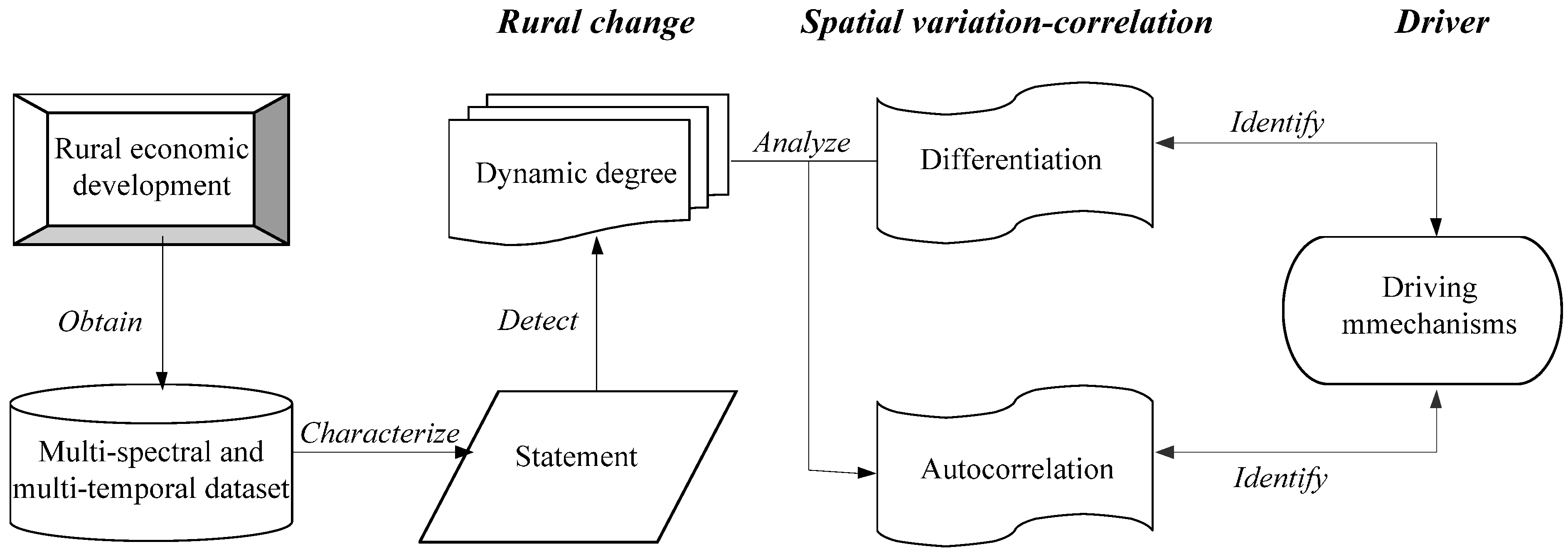
2.2. Analytical Framework

Devising the modeling framework, in practice, was based partly on the theoretical insights provided by previous research on rural economic performance and is remarkably similar to other approaches that have been used in subsequent studies [1]; notably, the Organization for Economic Co-operation and Development, OECD’s (2007) evaluation of economic differences amongst the regions of its member countries. However, the previous research mainly focused on a part of the statement (attitudes) of the rural development process, such as review differences in economic development in rural regions [4], food entrepreneurs [22], measurement of the determinants [1,23] and the factors [2] affecting rural development, and so on. Obviously, there is shortage of an analytical system to explain the characteristics of rural economic development, as shown in Figure 2.

Figure 2. The analytical framework for implementing rural development.

Figure 2. The analytical framework for implementing rural development.

2.3. Assessment Measures

Several measures have been chosen for the quantitative assessment of the dynamic degree and variation of rural economic development, including the Gini coefficient (G), Tsui–Wang index (TW) and Theil index (T). G, the most commonly-used measure of inequality, is more sensitive to assessing the differentiation of total income [24,25].

$$G=\frac{1}{2n^{2}u}{\displaystyle \sum _{j=1}^n{\displaystyle \sum _{i=1}^n\left|Y_j-Y_i\right|}}$$

(1)

where Y_i is each individual income in region i, similar to Y_j, n being the number of stylebooks, and u = mean income. The TW index, calculated based on Wolfson index, is used to depict a centralized character [26].

$$TW=\frac{\text{θ}}{N}{\displaystyle \sum _{i=1}^k{\pi }_i}{\left|\frac{y_i-m}{m}\right|}^r$$

(2)

where π_i is the number the population in region i and N is the total number of individuals. y_i is the GDP per capita in region i, and m is the middle GDP per capita of all regions. k is the number of provinces. θ and r are constants, and in this paper, θ = 1, r = 0.5. The TW scores are between 0 and 1. When TW is 1, the region is assumed to be completely polarized. In contrast, if TW is 0, the region is completely non-polarized.

The Theil inequality decomposition method is based on two Theil inequality indices, T and L [27,28]. Theil indices are additively decomposable and satisfy several desirable properties as a measure of regional income inequality, i.e., mean independence, population-size independence and the Pigou–Dalton principle of transfers [29,30].

$$T={\displaystyle \sum _i{\displaystyle \sum _j\left(\frac{Y_{ij}}{Y}\right)}}\log \left(\frac{Y_{ij}/Y}{N_{ij}/N}\right)$$

(3)

where Y_ij is the GDP of province j in region i, Y is the total GDP of the study area ($={\displaystyle \sum _i{\displaystyle \sum _j{Y}_{ij}}}$), N_ij is the population of province j in region i and N is the total population of all areas ($={\displaystyle \sum _i{\displaystyle \sum _j{N}_{ij}}}$).

If we define T_i as follows to measure between-province GDP inequality for region i,

$$T_i={\displaystyle \sum _j\left(\frac{Y_{ij}}{Y_i}\right)}\log \left(\frac{Y_{ij}/Y_i}{N_{ij}/N_i}\right)$$

(4)

then the Theil index T in Equation (4) can be decomposed into:

$$T={\displaystyle \sum _i\left(\frac{Y_i}{Y}\right)}{T}_i+{\displaystyle \sum _i\left(\frac{Y_i}{Y}\right)}\log \left(\frac{Y_i/Y}{N_i/N}\right)={\displaystyle \sum _i\left(\frac{Y_i}{Y}\right)}{T}_i+T_{BR}=T_{WR}+T_{BR}$$

(5)

where Y_i is the total GDP of region i ($={\displaystyle \sum _j{Y}_{ij}}$), N_i is the total population of region i ($={\displaystyle \sum _j{N}_{ij}}$) and $T_{BR}={\displaystyle \sum _i\left(\frac{Y_i}{Y}\right)}\log \left(\frac{Y_i/Y}{N_i/N}\right)$ measures GDP inequality between regions.

Equation (5) is the ordinary Theil inequality decomposition. T is the overall GDP inequality, and is also the sum of the within-region component (T_WR) and the between-region component (T_BR). The within-region component is a weighted average of the between-province GDP inequalities for each region (T_i).

2.4. Spatial Autocorrelation Model

The Moran index of spatial contiguity (Moran’s I) statistic, which is common in the analysis of spatial data [31,32], is the most venerable and widely-implemented tool for characterizing the spatial autocorrelation of areal units [33]. Moran’s I is generally defined as follows [34].

$$I=\frac{\left(1/S\right){\displaystyle \sum _i{\displaystyle \sum _{j}wij\left(ri-\overline{r}\right)\left(rj-\overline{r}\right)}}}{\left(1/N\right){\displaystyle \sum _i{\left(ri-\overline{r}\right)}^2}}$$

(6)

where r_i is the attribute value of region i and $\overline{r}$ is the mean value of the attributes of all regions. The factor w_ij is a weight that equals one if the distance of the variable r_i and r_j belongs to this interval and zero otherwise. S is the sum of weights for a given interval, and N is the total number of provinces. If I >0, under the given level of significance, it is a positive correlation, and the larger value indicates the greater relevance of the spatial distribution. If there is no spatial autocorrelation, the expected value of I is −1/(n − 1), which can be approximated by 0 if n is large.

Global Moran’s I can reveal spatial clusters of the regional economy and the neighbor effect of economic growth. According to LISA (Local Indicators of Spatial Association), patterns of local spatial cluster can be identified [35].

$$\begin{array}{l}Iit=\left(rit-ut\right){\displaystyle \sum _{j}Wij\left(rjt-ut\right)/S^2}\\ S^2={\displaystyle \sum _i{\left(rit-ut\right)}^2/n}\end{array}$$

(7)

where I_it is local Moran’s I statistics of the region i in year t, r_it is the attribute value of the region i in year t, u_t is the mean of all regional attribute values, n is the number of regions and S² is the sample variance. If I_it > 0, region i has a local positive correlation with other regions, and I_it < 0 shows negative correlation. A multiple-sequences Monte Carlo simulation test is used to test the significant level of LISA [35]. A small p-value (p < 0.05) indicates that the neighbor effect of region i is relatively high, while a large p-value (p > 0.95) indicates that it is relatively low [36].

3. Results

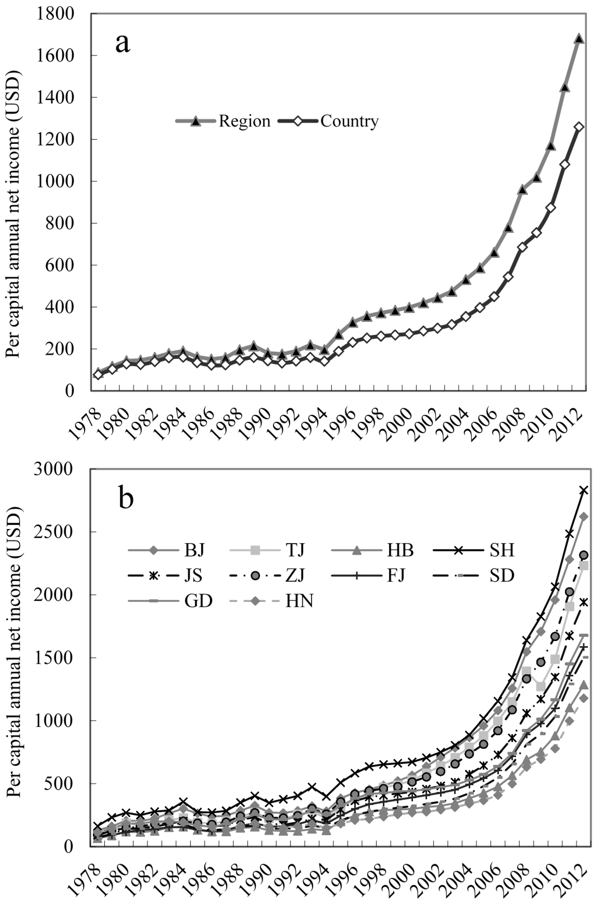
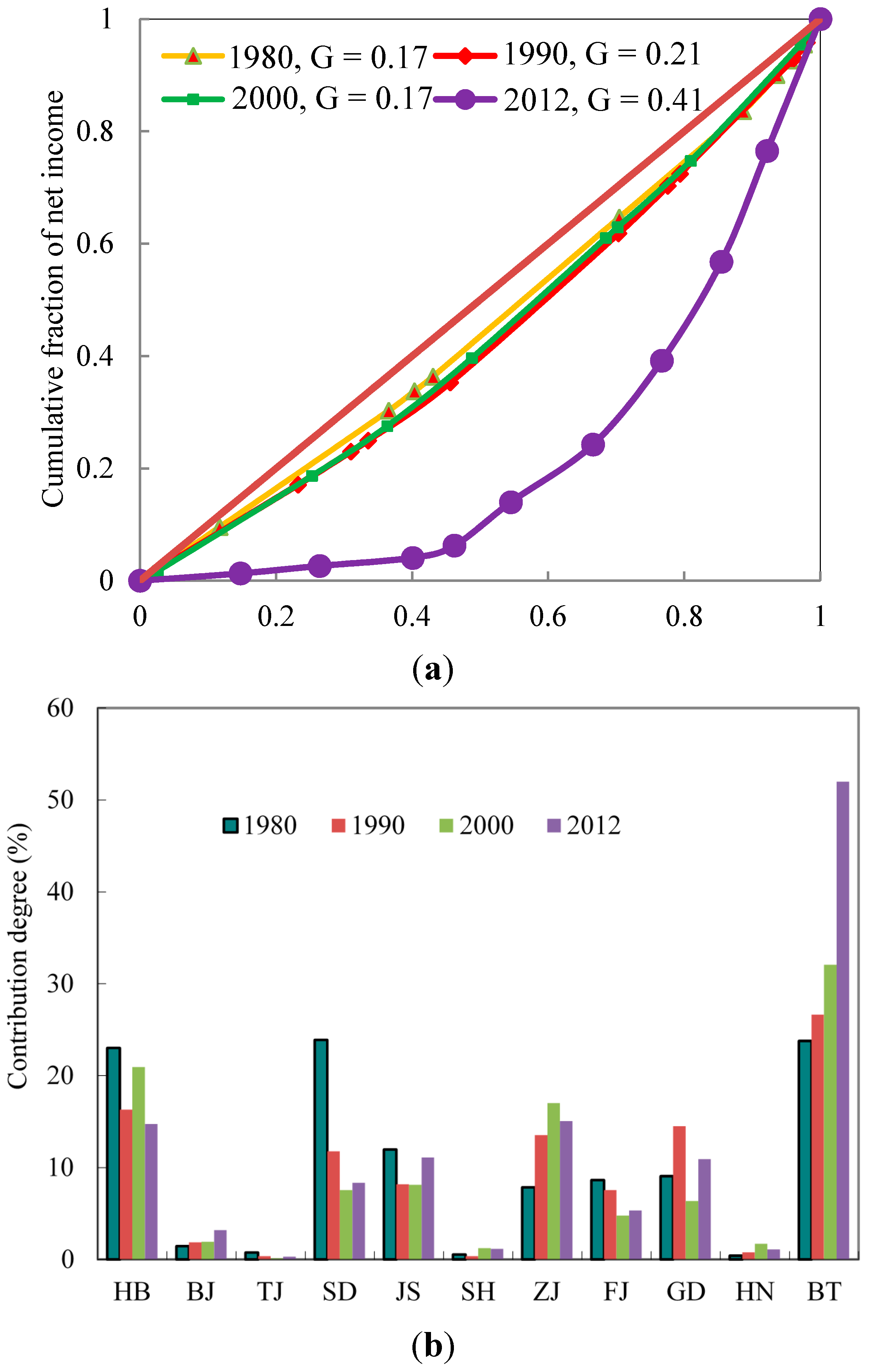
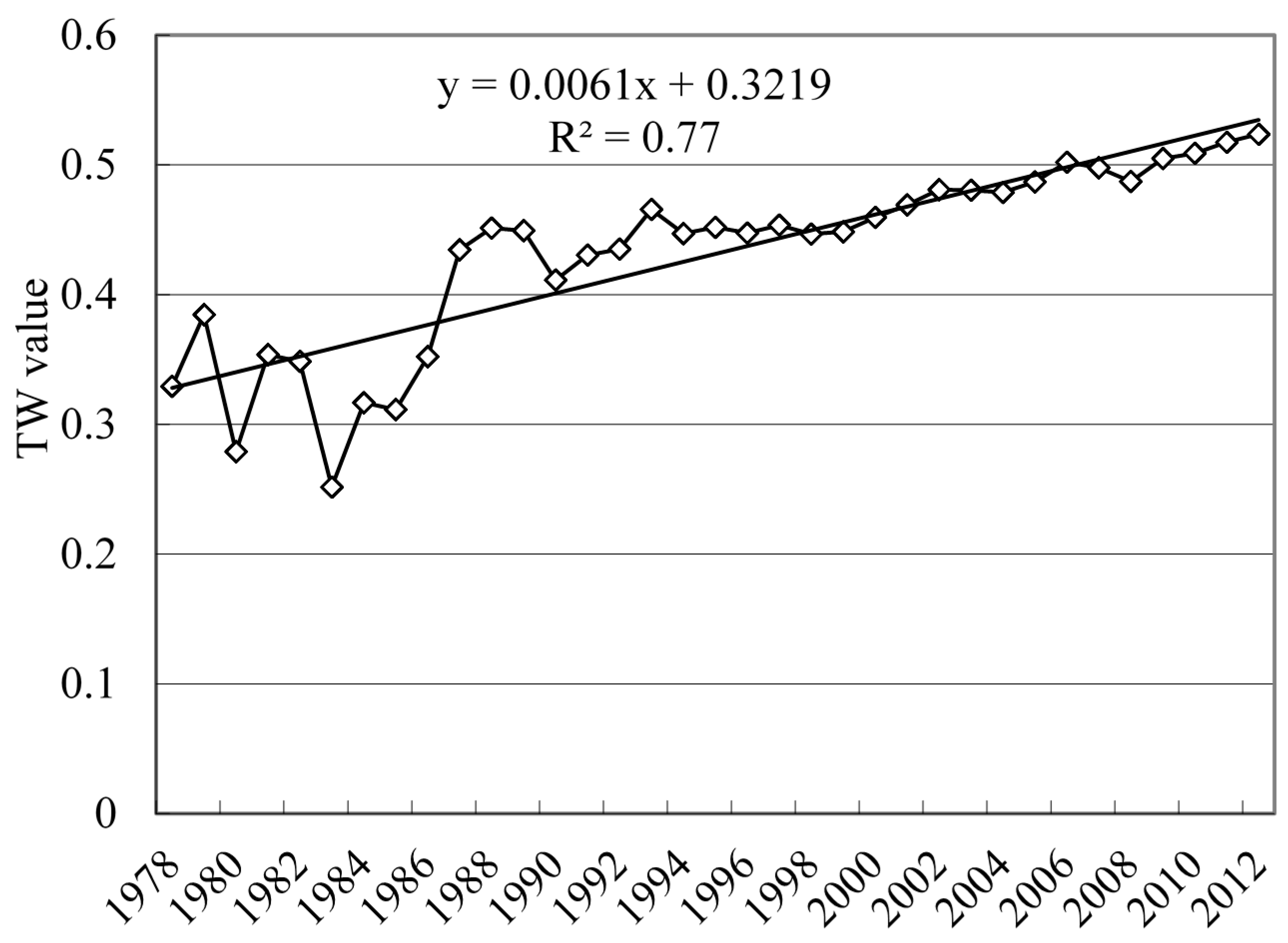
3.1. Dynamic Variation of Rural Development

The per capita annual net income was found to have changed significantly over the entire period, from 1978 to 2012 in the eastern coastal region of China, as shown in Figure 3. In accordance with the growth rate of net income, the entire process can be divided into three stages. The first period, which is from 1978 to 1996, as well as the third period of 2004 to 2012 are rapid growth step periods, in which the growth rate was more than 10%. The second stage, ranging from 1997 to 2003, is a slow growth period, as illustrated in Figure 3. During the focus period in this study, ranging from 1978 to 2012, the value of the income per capita increased 18 times, from 87.7 to 1628.1 USD. In view of the overall situation, the annual net income of the study regions was found to be higher than the national average level, and the gap is becoming progressively larger, as shown in Figure 3a.

On a provincial level, the trends of the per capita annual net income of rural households were very similar and almost synchronous. However, when grouping the phenomenon and differentiation, they were very distinct. It was apparent that Shanghai, Beijing, Tianjin and Zhejiang belonged to the first group, with the average value of more than 2200 USD in 2012. The next group included Jiangsu, Guangdong, Fujian and Shandong, and the third group contained the two provinces of Hebei and Hainan. Their per capita annual net income was below 1500 USD. The gap between the provinces changed slowly during the period ranging from 1978 to 1991. However, it has become larger since 1992, as shown in Figure 3b.

Figure 3. The contrast and evolution trends of annual net income in eastern coastal rural areas during the period of 1978 to 2012 (HB, Hebei; BJ, Beijing; TJ, Tianjin; SD, Shandong; JS, Jiangsu; SH, Shanghai; ZJ, Zhejiang; FJ, Fujian; GD, Guangdong; HN, Hainan; the meanings of the abbreviations in other parts of the manuscript are the same). (a) at the national and regional level; (b) at provincial level.

Figure 3. The contrast and evolution trends of annual net income in eastern coastal rural areas during the period of 1978 to 2012 (HB, Hebei; BJ, Beijing; TJ, Tianjin; SD, Shandong; JS, Jiangsu; SH, Shanghai; ZJ, Zhejiang; FJ, Fujian; GD, Guangdong; HN, Hainan; the meanings of the abbreviations in other parts of the manuscript are the same). (a) at the national and regional level; (b) at provincial level.

In accordance with the average rural economic development levels of 60%, 100% and 150%, the study region can be divided into four categories: areas with more than the average level of 150% belong to Type I (rural developed regions); areas between 100% and 150%, between 60% and 100%, and less than 60% are shared by Type II (rural medium to high developed regions); followed by Type III (rural moderately developed regions); and Type IV (rural underdeveloped regions); as shown in Figure 4.

Figure 4. The types of rural development levels in eastern coastal China.

Figure 4. The types of rural development levels in eastern coastal China.

Prior to 2000, the majority of China’s eastern coastal regions belonged to underdeveloped and moderately developed rural areas, which accounted for more than half of the total area. However, the areas of Type I and Type II were much less. Since 2000, China’s rural eastern coastal regions have achieved rapid economic development, and regional diversity rules have been increasingly displayed. During this period, an increasing number of areas moved into the Type I and Type II categories. This indicated that most of the rural regions entered a medium developed level. A number of county units were located in the more developed regions, and the developed regions showed obvious growth. By 2012, an integral pattern of regional rural development had been fundamentally formed.

The category Types I and II were mainly located at the junction of Beijing, Tianjin and Hebei, central and eastern Shandong, the Yangtze River Delta, south-central Guangdong and parts of Fujian Province. Due to rapid industrialization and urbanization in these areas, the highly developed business, tourism and other service industries played important roles in promoting the local rural development, both from the aspect of industry and employment.

The category Types III and IV were mainly located in northern Hebei Province, southern and western Shandong, northern Jiangsu, western Fujian, southwestern Guangdong and most parts of Hainan. These areas, which were mainly located in the remote and mountainous areas, with higher ecological service value, were the planting areas of primary agricultural products. Therefore, due to poor location situations, the rural economic development in these categories was very slow.

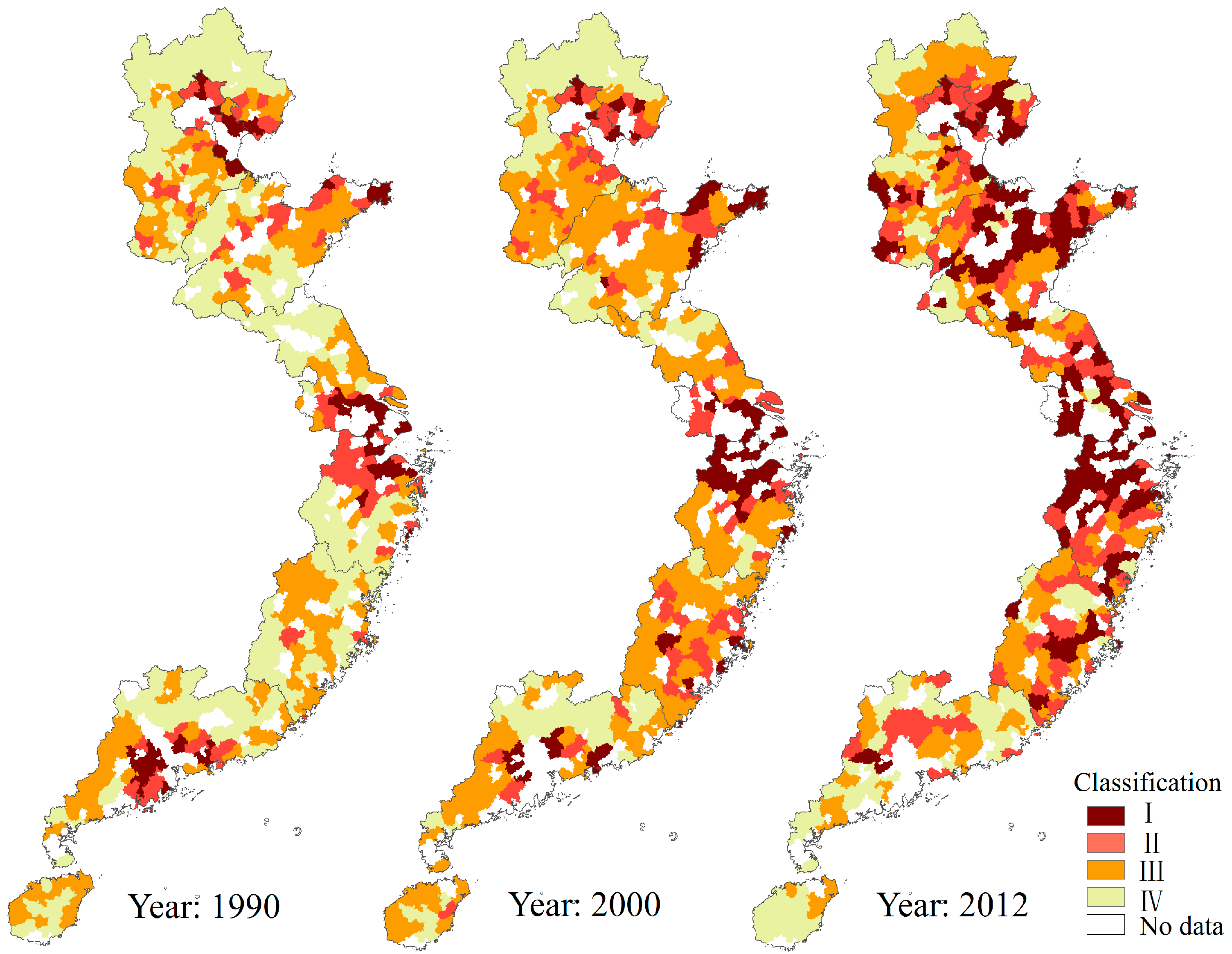
3.2. Spatio-Temporal Differences in the Eastern Coastal Area

The evaluation of the spatio-temporal differences in the eastern coastal area was conducted for three indices (G, TW and T). Figure 5 shows that before the year 2000, the differentiation of the entire per capita income range is very small throughout the study area, which was derived by calculating the index G according to Formula (1), and the G-value was always in a reasonable interval. However, the regional polarization continuously strengthened, while the G-value reached 0.41 in 2012. This suggested that the regional differences were major and exceeded a reasonable range. During the period from 1978 to 2012, the trend of the TW-value was obviously rising. The TW index reached the maximum value of 0.52 in 2012 and the minimum value of 0.252 in 1983, as illustrated in Figure 6.

Figure 5. Changes of G (Gini) and T (Theil) indexes in eastern coastal China. (a) Gini; (b) Theil.

Figure 5. Changes of G (Gini) and T (Theil) indexes in eastern coastal China. (a) Gini; (b) Theil.

Figure 6. Changes of the TW (Tsui–Wang) index in eastern coastal China during 1978–2012.

Figure 6. Changes of the TW (Tsui–Wang) index in eastern coastal China during 1978–2012.

Due to the differences in resource predominance and development environments, the provincial differences are becoming increasingly serious. The areas located in Beijing, Tianjin and Shanghai focus on business, tourism and providing services, whereas rural development mainly depends on tertiary industries. In these areas, the per capita annual net income of the rural households was higher than that of those people who live in the remote and mountainous areas, where the agriculture-oriented industries dominated rural economic development to some extent.

Similarly, the gap was relatively minor in the same province, due to the similarity of policies and developmental conditions. In addition, government regulations also play important roles in balancing the regional development. As a result, the overall gap in the per capita annual net income was found to be shrinking in the same province, as shown in Figure 5.

3.3. Spatial Autocorrelation Analysis of Rural Development

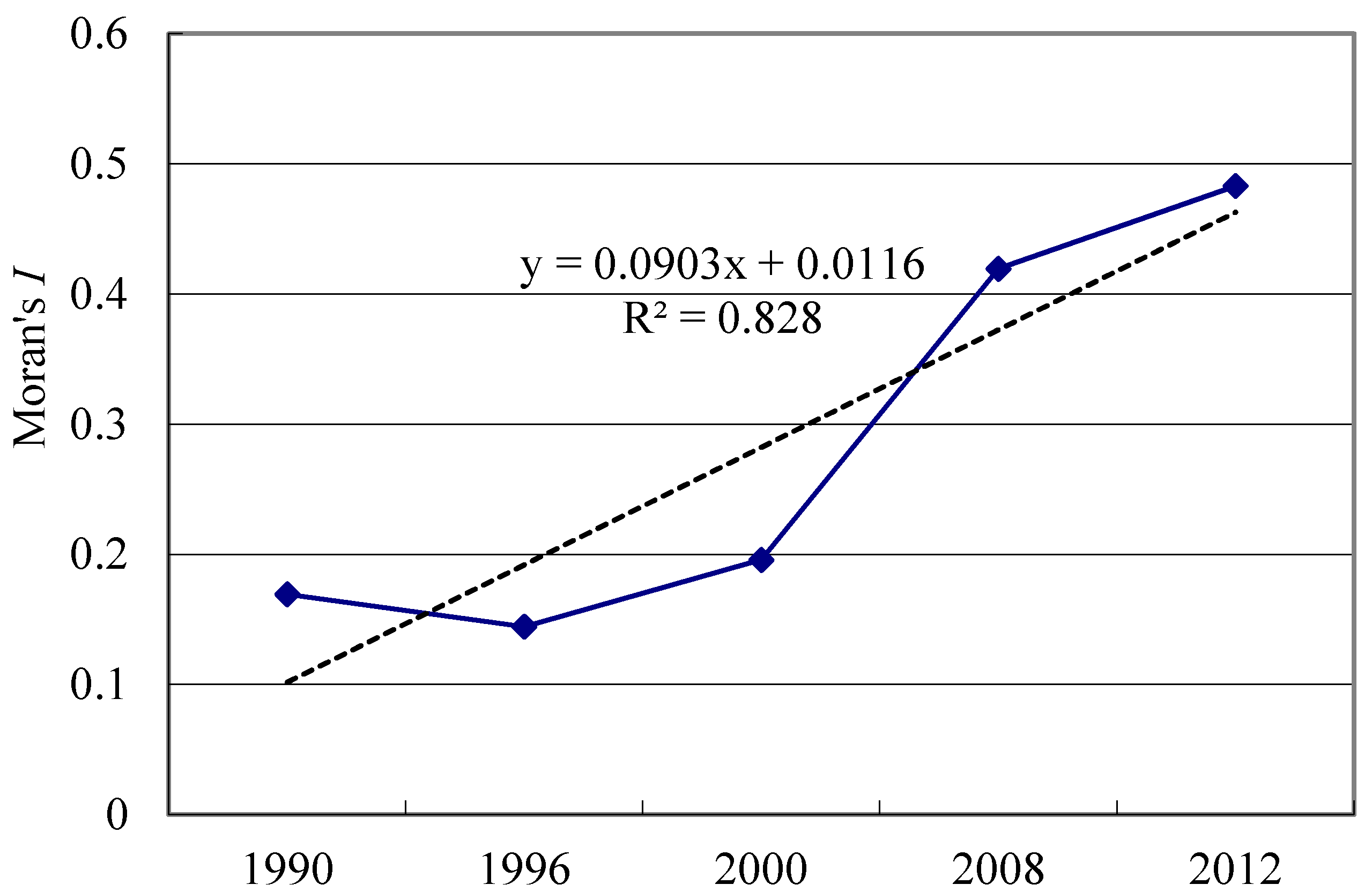
3.3.1. Analysis of Global Spatial Autocorrelation

According to a one-sample Kolmogorov–Smirnov (K-S) test, the data from 1990 to 2012 followed a normal distribution, and the effectiveness of the data has been verified. Table 1 illustrated that Z(I) > Zα > 0, which demonstrates that the county per capita GDP has an appositive spatial autocorrelation at a 1% significance level.

The Moran I-value, calculated according to Formula (6), represents the degree of spatial autocorrelation of areal units. Table 1 and Figure 7 show that the Moran I-value rose with a waving trend from 1990 to 2012 (Figure 7), which suggests that the spatial clusters of the regional economy were significant, and the neighbor effect was continuously strengthened.

The variation trends of aggregation in the eastern regions, beginning in 1990 to 2012, were fit using functions, and the results suggested that the variation trend during this period agrees well with the linear fitting curve, with the degree of fitting reaching as high as 0.828.

Table 1. Estimates of global Moran’s I per capita GDP in eastern coastal China.

Year	1990	1996	2000	2008	2012
Moran’s I	0.17	0.14	0.20	0.42	0.48
Z Score	6.41	5.47	7.40	15.89	18.32
Variance	0.0007	0.0007	0.0007	0.0007	0.00068
p-Value	0.001	0.001	0.001	0.001	0.001

Table 1. Estimates of global Moran’s I per capita GDP in eastern coastal China.

Year	1990	1996	2000	2008	2012
Moran’s I	0.17	0.14	0.20	0.42	0.48
Z Score	6.41	5.47	7.40	15.89	18.32
Variance	0.0007	0.0007	0.0007	0.0007	0.00068
p-Value	0.001	0.001	0.001	0.001	0.001

Figure 7. Values of the global spatial autocorrelation coefficient in eastern coastal China.

Figure 7. Values of the global spatial autocorrelation coefficient in eastern coastal China.

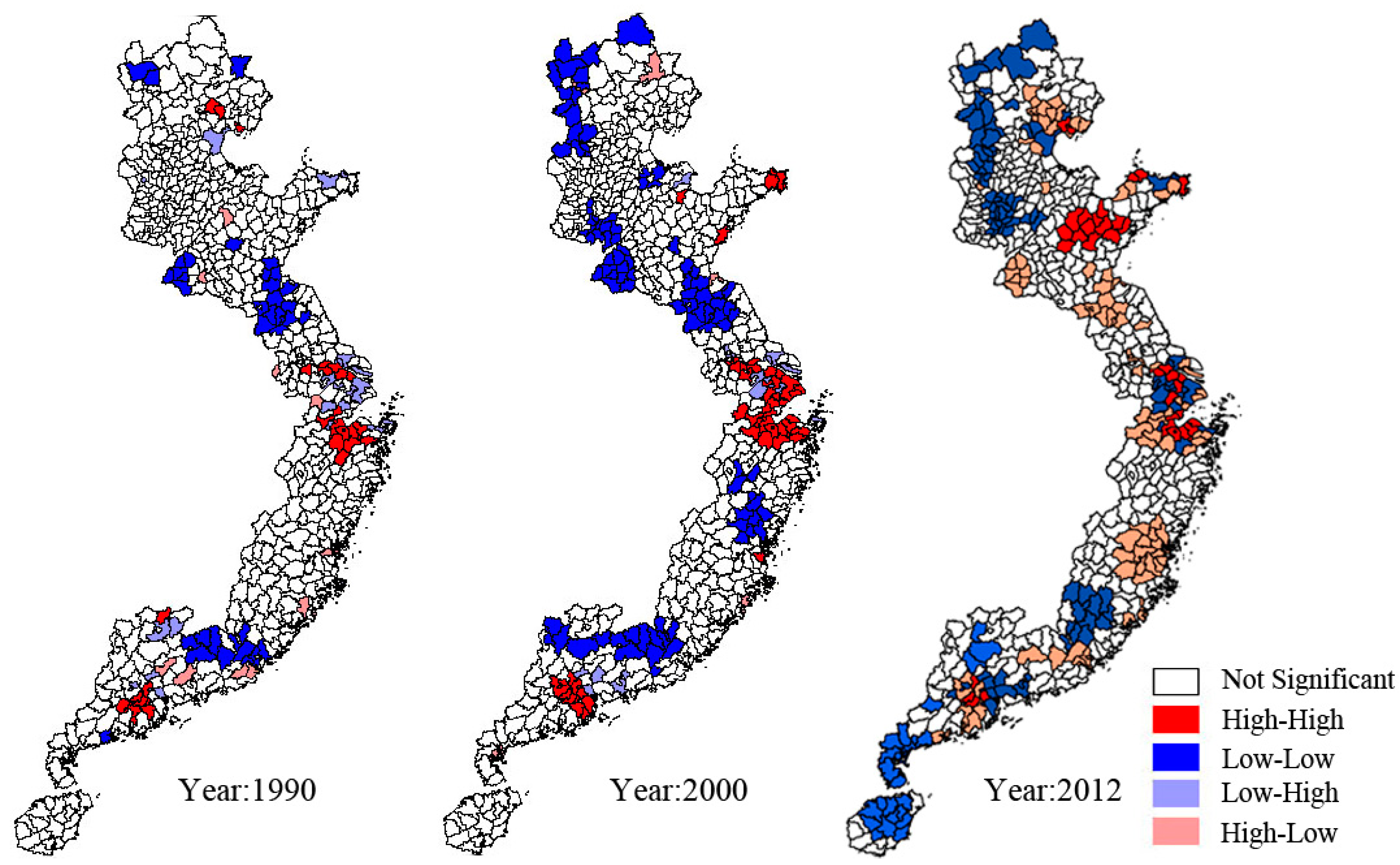
3.3.2. Analysis of Local Spatial Autocorrelation

At the county level, the features of the local spatial autocorrelation, which were analyzed by Geoda 095i and ArcGIS 9.3 software, were classified into four types. The first type was high-high, which represented regions with high value surrounded by neighbors of high value. The second type was low-low, signifying low value surrounded by neighbors of low value, both of which showed a positive correlation. The low-high group was the third type, representing the regions with low value surrounded by neighbors of high value. Finally, the last type was the high-low group, with high value surrounded by neighbors of low value, both of which showed a negative correlation [36].

Figure 8 illustrates that, in the process of rural economic development, space differentiation was very significant. These results were derived from the scatter plot map, according to the various economic units per capita GDP of the LMI (Local Moran’s I) value and plotted at a p < 0.05 level.

The concentration trends of both the high-high and low-low types were apparent in the areas that were increasing. Actually, partial areas of the low-high types gradually turned into high-high types during the period from 1990 to 2012. When the conditions in 2012 are set as an example, the high-high types were mainly located in the Yangtze River Delta, south-central Guangdong and central and eastern Shandong. The low-low types experiencing low growth were distributed in western and southern Hebei, southern Fujian, southwestern Guangdong and most parts of Hainan (Figure 8: year 2012). The areas of low-high and high-low category types were relatively small and changed only slightly during the period ranging from 1990 to 2012. The low-high types also surrounded the high-high types, especially in the Pearl River Delta.

Figure 8. Distribution of rural economic spatial autocorrelation patterns in eastern coastal China.

Figure 8. Distribution of rural economic spatial autocorrelation patterns in eastern coastal China.

4. Discussion

In order to explain the causes of spatio-temporal differentiation characteristics in rural economic development, three factors were analyzed, namely resource endowments, economic location and policies as driving mechanisms, which were the fundamental driving factors affecting the regional differences.

4.1. Resources Endowment

The natural factors referred to as the resource endowments were the first factor. Resource endowments are fundamental and important supporting conditions for rural and agricultural development in the initial developmental periods. This is due to the fact that the resource endowments include solar heat, water and soil resources, on which agriculture is dependent. Resource endowments also play an important role in the regional division as a standard. The areas with good resource endowments developed more efficiently than the regions with poor resource endowments and achieved primitive accumulation. Furthermore, the original equilibrium development pattern became broken, and the regional development’s first deviation appeared.

4.2. Economic Location

According to path dependence theory, having a good economic location, such as the countryside near the central cities, with convenient transportation conditions and proximity to transportation hubs, are very conducive to the development of a rural economy [37]. The cities, which are the regional centers, play a greater role at improving the traditional agricultural structural transformation of their surrounding rural areas than they do for the remote regions. Therefore, regional centers, such as in southern Jiangsu (Su-nan), referred to as the “Su-nan model”, have a significant impact on the development of rural industries based on the diversified collective enterprises operated by the local municipality model [38,39]. Their agricultural structure transmitted quickly, following the trends of nearby cities with rapid industrialization and urbanization and developed faster than the areas with poor economic locations. In other words, the distance to the market directly affects income level per capita. Additionally, this point had been proven right by Yilmaz, who chose Bartın in Turkey as a case study by means of a multi-dimensional approach.

4.3. Policy Factors

Policies formulated by the government are the third factor that contributed to the rural development deviations. With the widening gap in the regional development, social conflicts were aggravated, which went against the Construction of a Harmonious Society. In order to avoid intense conflict and to shrink the regional differences, the government had the responsibility to create preferential policies and agricultural subsidies that were applicable to the under-developing areas. Furthermore, the adoption of a new country-side policy was carried out by the government. Many studies are the proofs of the success of these reform policies. As Long et al. [40] described it, rural development policies reached their anticipated goals to coordinate urban and rural development overall and to gear up national economic growth.

With the period of the industries supporting agriculture and the cities supporting the countryside approaching, many measures and policies have been formulated and implemented by our government in order to emphatically increase the income of farmers. However, we should not ignore that a farmer, as a subject status, is the core of rural development. In general, improving our farmers’ quality of life is as important as increasing our farmers’ income. Therefore, the development of rural education will not only improve farmers’ quality of life, but it also will become a fundamental solution to the “three rural” key issues. This is also conducive to the transfer of rural labor and will ultimately achieve a rapid development of the rural economy. In addition, in regards to the ecological protection areas, as well as the food security areas, our government should establish a sound compensation system and ensure that the comparative advantages are in full play in all regions. This is also referred to as staggered development.

5. Conclusions

In eastern coastal China, with its rapid urbanization and industrialization, rural economic development has been greatly influenced. The per capita annual net income has changed significantly over the period ranging from 1978 to 2012. The annual net income of the study region was higher than the national average level, and this gap presented an aggregate trend similar to the gap among the provinces. On the other hand, the entire level of rural economic development in the eastern coastal areas constantly improved, and areas increasingly progressed to medium and advanced levels.

The spatio-temporal differentiation characteristics of the rural economic development in the eastern coastal regions of China are very significant. In the spatio-temporal differences of eastern coastal areas, the differentiation of the entire per capita incomes was generally very small throughout the study area. However, the regional polarization continuously strengthened. In other words, the provincial differences were increasingly serious during the period of 1978 to 2012.

According to the analysis of the spatial autocorrelation of rural development, we found that the spatial clusters of the regional economy were significant, and the neighbor effect was continuously strengthened. On a county level, the space differentiation was very significant, which was derived from a scatter plot map. The concentration trends of both the high-high types and the low-low types were apparent, with these areas showing increases. The high-high types were mainly located in the Yangtze River Delta, south-central Guangdong and central and eastern Shandong, while the low-low types were distributed in western and southern Hebei, southwestern Shandong, northern Jiangsu, the north of Zhejiang, southwestern Guangdong and most parts of Hainan and Fujian. The areas of low-high and high-low category types were relatively small and changed only slightly during the period of 1990 to 2012.

Location was a significant factor affecting rural economic development. First of all, on a macroscopic scale, if the studied regions or countries paid attention to rural economic development (it should be noted that agriculture is an important basis for rural development), then there were more policies in place that were beneficial to rural development, thus the rural economy could develop well. If no attention was paid, then the rural economy was underdeveloped. Secondly, the position of the province had an effect on the rural economic development. However, the prerequisite was that the provinces should give emphasis to rural economic development. If this occurred, then the rural economy in the provinces developed well; otherwise, the rural economy was underdeveloped.

References

1. Agarwal, S.; Rahman, S.; Errington, A. Measuring the determinants of relative economic performance of rural areas. J. Rural Stud. 2009, 5, 309–321. [Google Scholar] [CrossRef]
2. Yilmaz, B.; Daşdemir, I.; Atmis, E.; Lise, W. Factors affecting rural development in turkey: Bartın case study. For. Policy Econ. 2010, 12, 239–249. [Google Scholar] [CrossRef]
3. Long, H.L.; Zou, J.; Liu, Y.S. Differentiation of rural development driven by industrialization and urbanization in eastern coastal China. Habitat Int. 2009, 33, 454–462. [Google Scholar] [CrossRef]
4. Terluin, I.J. Differences in economic development in rural regions of advanced countries: An overview and critical analysis of theories. J. Rural Stud. 2003, 19, 327–344. [Google Scholar] [CrossRef]
5. Hayati, D.; Karbalaee, F. Revising agricultural development by rethinking rural development strategy in Iran. Tech. J. Eng. Appl. Sci. 2013, 3, 1411–1417. [Google Scholar]
6. Sanderson, S. Poverty and conservation: The new century’s “Peasant Question?”. World Dev. 2005, 33, 323–332. [Google Scholar] [CrossRef]
7. Courtney, P.; Hill, G.; Roberts, D.; Deborah, R. The role of natural heritage in rural development: An analysis of economic linkages in Scotland. J. Rural Stud. 2006, 22, 469–484. [Google Scholar] [CrossRef]
8. Lise, W. An Econometric and Game Theoretic Model of Common Pool Resource Management: People’s Participation in Forest Management in India; Nova Science Publishers Inc.: Hauppauge, NY, USA, 2007. [Google Scholar]
9. Narain, U.; Gupta, S.; Veld, K.V. Poverty and resource dependence in rural India. Ecol. Econ. 2008, 66, 161–176. [Google Scholar] [CrossRef]
10. Long, H.L.; Zou, J.; Pykett, J. Analysis of rural transformation development in China since the turn of the new millennium. Appl. Geogr. 2011, 31, 1094–1105. [Google Scholar] [CrossRef]
11. Peng, Y.S. What has spilled over from Chinese cities into rural industry? Mod. China 2007, 33, 287–319. [Google Scholar] [CrossRef]
12. Kadri, S. Neighborhood milieu in the cultural economy of city development: Berlin’s Helmholtzplatz and Soldiner in the German “Social City” program. Cities 2011, 28, 95–106. [Google Scholar] [CrossRef]
13. Cheng, Z.M.; Wang, H.N. Do neighborhoods have effects on wages? A study of migrant workers in urban China. Habitat Int. 2013, 38, 222–231. [Google Scholar] [CrossRef]
14. Michele, M.; Annalisa, D.B.; Rocco, R. Economic and environmental sustainability of forestry measures in Apulia Region Rural Development Plan: An application of life cycle approach. Land Use Policy 2014, 41, 284–289. [Google Scholar] [CrossRef]
15. Toivo, M. Needs for rural research in the northern Finland context. J. Rural Stud. 2010, 26, 73–80. [Google Scholar] [CrossRef]
16. Liu, Y.S.; Wang, L.J.; Long, H.L. Spatio-temporal analysis of land-use conversion in the eastern coastal China during 1996–2005. J. Geogr. Sci. 2008, 18, 274–282. [Google Scholar] [CrossRef]
17. National Bureau of Statistics of China. China Statistical Yearbook (1996–2013); China Statistics Press: Beijing, China, 1996–2013. [Google Scholar]
18. National Bureau of Statistics of China. China Compendium of Statistics; China Statistics Press: Beijing, China, 2009. [Google Scholar]
19. National Bureau of Statistics of China. Comprehensive Statistical Data and Materials on 50 Years of New China; China Statistics Press: Beijing, China, 1999. [Google Scholar]
20. National Bureau of Statistics of China. China County Statistical Yearbook (2001–2013); China Statistics Press: Beijing, China, 2001–2013. [Google Scholar]
21. National Bureau of Statistics of China. China Rural Statistical Yearbook (1985–2013); China Statistics Press: Beijing, China, 1985–2013. [Google Scholar]
22. Ilberya, B.; Watts, D.; Little, J.; Gilga, A.; Simpsond, S. Attitudes of food entrepreneurs towards two grant schemes under the first England Rural Development Programme, 2000–2006. Land Use Policy 2010, 27, 683–689. [Google Scholar] [CrossRef]
23. Vennesland, B. Measuring rural economic development in Norway using data envelopment analysis. For. Policy Econ. 2006, 7, 109–119. [Google Scholar] [CrossRef]
24. Alvaredo, F. A note on the relationship between top income shares and the Gini coefficient. Econ. Lett. 2011, 110, 274–277. [Google Scholar] [CrossRef]
25. Zheng, B.H.; Brian, C. Statistical inference for testing inequality indices with dependent samples. J. Econom. 2001, 101, 315–335. [Google Scholar] [CrossRef]
26. Wang, Y.Q.; Tsui, K.Y. Polarization orderings and new classes of polarization indices. J. Public Econ. Theory. 2000, 2, 349–363. [Google Scholar] [CrossRef]
27. Theil, B.H. The information approach to demand analysis. Econometrica 1965, 33, 67–87. [Google Scholar] [CrossRef]
28. Akita, T. Decomposing regional income inequality in China and Indonesia using two-stage nested Theil decomposition method. Reg. Sci. 2003, 37, 55–77. [Google Scholar] [CrossRef]
29. Bourguignon, B.F. Decomposable income inequality measures. Econometrica 1979, 47, 901–920. [Google Scholar] [CrossRef]
30. Shorrocks, B.A.F. The class of additively decomposable inequality measures. Econometrica 1980, 48, 613–625. [Google Scholar] [CrossRef]
31. Dale, M.R.T.; Fortin, M.J. Spatial autocorrelation and statistical tests in ecology. Ecoscience 2002, 9, 162–167. [Google Scholar]
32. Legendre, P. Spatial autocorrelation: Trouble or new paradigm? Ecology 1993, 74, 1659–1673. [Google Scholar] [CrossRef]
33. O’Sullivan, D.; Unwin, D.J. Geographic Information Analysis; Wiley Press: New York, NY, USA, 2003. [Google Scholar]
34. Shortridge, A. Practical limits of Moran’s autocorrelation index for raster class maps. Comput. Environ. Urban Syst. 2007, 31, 362–371. [Google Scholar] [CrossRef]
35. Anselin, L. Local indicators of spatial association-LISA. Geogr. Anal. 1995, 27, 93–115. [Google Scholar] [CrossRef]
36. Qiao, X.N.; Yang, D.G.; Zhang, X.H. Evolution stages of oasis economy and its dependence on natural resources in Tarim River Basin. Chin. Geogr. Sci. 2009, 19, 265–273. [Google Scholar] [CrossRef]
37. Liu, Y.S.; Wang, G.G.; Zhang, F.G. Spatio-temporal dynamic patterns of rural area development in eastern coastal China. Chin. Geogr. Sci. 2013, 23, 173–181. [Google Scholar] [CrossRef]
38. Tan, K. Revitalized small towns in China. Geogr. Rev. 1986, 76, 138–148. [Google Scholar] [CrossRef]
39. Xie, Y.C.; Batty, M.; Zhao, K. Simulating emergent urban form using agent based modeling: Desakota in the Suzhou-Wuxian region in China. Ann. Assoc. Am. Geogr. 2007, 97, 477–495. [Google Scholar] [CrossRef]
40. Long, H.L.; Liu, Y.S.; Li, X.B. Building new countryside in China: A geographical perspective. Land Use Policy 2010, 27, 457–470. [Google Scholar] [CrossRef]