A Stackelberg Game Approach in an Integrated Inventory Model with Carbon-Emission and Setup Cost Reduction

Abstract

This paper formulates an integrated inventory model that allows Stackelberg game policy for optimizing joint total cost of a vendor and buyer system. After receiving the lot, the buyer commences an inspection process to determine the defective items. All defective items the buyer sends to vendor during the receiving of the next lot. Due to increasing number of shipments fixed and variable transportation, as well as carbon emissions, are considered, which makes the model sustainable integrated model forever. To reduce the setup cost for the vendor, a discrete setup reduction is considered for maximization more profit. The players of the integrated model are with unequal power (as leader and follower) and the Stackelberg game strategy is utilized to solve this model for obtaining global optimum solution over the finite planning horizon. An illustrative numerical example is given to understand this model clearly.

1. Introduction

Generally, an integrated-production-inventory model defines the vendor-buyer or retailer-customer model. In that type of model, usually a vendor produces an item in a production batch line and the produced finished goods are transferred to several buyers. In spite of that, retailer’s production cycle time is measured as an integer multiple of the function of consumer’s ordering time. Many research articles highlighted various integrated vendor-buyer models with several key parameters. Chang et al. [1] discussed an integrated vendor-buyer inventory system under trade-credit policies. Demand is measured as the diminishing function of retail-price. Additionally, they surveyed an iterative algorithm to figure out the optimal retail-price, number of buyer’s ordering amount, and numbers of deliveries per production run. Yang [2] extended previous research models considering an integrated-inventory model with lead time crashing cost. Hoque [3] analyzed a vendor-buyer integrated-production model, where lead time follows a normal distribution along with setup time of a machine, maximum boundary on capacity of shipping vehicle, cost of transportation, and batch time are also inserted in his model. Jha and Shanker [4] established an integrated inventory model with transportation for a single-vendor and multi-buyer. It is observed that the vendor produces and deliveries products to buyers in distinct locations by similar capability of some vehicles. The external demands of buyers are taken to be independent and follows a normal distribution. Lead time of buyers without transportation time are reduced by an added crashing cost. Most of the above mentioned research articles related to the integrated-inventory model are formed with the assumption that all produced items are absolutely perfect. There are no defective items during production system. Sarkar et al. [5] expanded former integrated-inventory models by including the concept of imperfect production. An inspection policy is given to examine defective items and also provides delay-in-payments in their model. In their model, non-defective item follows a binomial distribution and lead time demand follows a mixture of normal distribution. By highlighting the trade-credit policy, Ouyang et al. [6] derived an integrated-inventory model with a capacity constraint and a permissible delay-payment system. An unit production cost is calculated as the function of rate of production. Sarkar et al. [7] analyzed a continuous review inventory model on the basis of probability distribution of lead time demand. Some investment function is applied to improve the process quality. They presented two models, one with normal distributed lead time demand and another with an unknown distributed lead time demand. Sarkar [8] discovered a vendor-buyer model by considering three steps of inspection process before vendor’s consignment. Ahmad et al. [9] formulated an integrated-inventory model which includes single-supplier, single-manufacturer, and single-retailer. In addition, imperfect production process is also considered in their model. Fauza et al. [10] provided a single-vendor and multiple buyers (SVMB) model to obtain the food inventory policy. They developed a kinetic model, which is utilized to present the quality degradation of the raw material at the vendor. In literature, there are several integrated inventory models, but no one of the above mentioned authors considered unequal power of player in the integrated model. Every model is considered to have equal power of the players. However, if the players are with unequal power then only game strategy (using leader-follower policy) can be used those models.

In many Stackelberg approaches, decision makers are always in the leading positions to obtain more profit jointly or individually. Those Stackelberg game models consider the assumption that leader first selects his decisions and then those decisions are becoming the constraint to the follower. Besides, concept of follower’s decision makes on the whole data of the leader’s action and his decisions turn the new constraints to that leader’s decision problem. Liou et al. [11] described some multi-period inventory models which consists of one-buyer and one-seller. They highlighted the Stackelberg equilibrium framework for maximizing vendor’s total benefit with respect to the minimum total cost that the buyer is willing to obtain. Yu et al. [12] showed how a manufacturer and its retailers are related with each other in order to optimize their individual total profits. They considered the fact that the manufacturer develops a single product at the same wholesale price to multiple retailers. After that, those multiple retailers sell that product in independent markets at some retail prices. In addition, they assumed that the demand rate is an increasing as well as concave function of advertising investments of both local retailers and the manufacturer while a decreasing and convex function of the retail prices. Yu et al. [13] formulated an integrated inventory model in which Stackelberg game is incorporated to increase vendor’s profit in a vendor managed inventory (VMI) system. In their paper, vendor is assumed to be as a manufacturer who produces raw materials to develop a finished product and then distributed it to multiple retailers at the same wholesale price. Then, the retailers sell the product in independent markets at retail prices. Zhou and Zhou [14] proposed a two-echelon supply chain which states that a supplier sells through a retailer a product with some stable market demand. By using some ‘supplier-Stackelberg’ setting, they observed two trade credit scenarios which are unconditional and conditional. They also provided that unconditional trade credit scenario is always profitable to the retailer but harmful to the supplier. On other hand, conditional trade credit scenario is always profitable to both parties. Wang et al. [15] provided a win-win outcome for his Stackelberg game model. By examining two decision makers of that game, supplier along with a threshold and partial trade-credit policy is considered to adjust that model. Taleizadeh et al. [16] described a Stackelberg game-theoretic approach in a composite (QFF) policy which consists of quantity, freight discount, and free shipping quantity policies. In their paper, they assumed that supplier offers some composite policy and manufacturer offers some composite (QPR) policy to the retailers. Wang et al. [17] addressed a product family architecture (PFA) planning and supply chain configuration as a Stackelberg game approach. They presented the PFA decision making as an upper-level optimization problem. On the other side, the lower-level optimization problem deals with the supply chain decisions. Though there are several models considering Stackelberg game policy, but no one considered this strategy for integrated inventory model for unequal lot size within single-setup-multi-delivery policy. This research gap is fulfilled by the proposed research model.

Setup cost plays an important role in today’s advanced manufacturing companies for shipment of products on time. Setup process is not measured as a value adding constraint. Setup cost need to be discussed at the time of enhancing productivity, minimizing waste, enlarging resource utilization, and satisfy deadlines. To minimize capital investment function, manufacturer are required to reduce setup cost. Researchers made various inventory models with this concept of setup cost reduction. Denizel et al. [18] studied a dynamic lot size model in which setup costs can be reduced by several amounts depending upon the level of raw-materials. They also derived a shortest path problem for these level of raw-materials. Diaby [19] established a comprehensive model to reduce both setup time and setup cost. He also added that setup times can be reduced by contributing appropriate amounts of many resources like equipment, tooling, etc. He determined how much to cut setup time for every product and how much of each good to manufacture to minimize total cost. Nyea et al. [20] developed some inventory models to forecast optimal setup times, or optimal investment in setup reduction. In their paper, a new model based on queuing theory was formed to estimate work-in-process (WIP) levels. Freimer et al. [21] established two types of process improvements which are (i) setup costs reduction; and (ii) improvement in quality of the process. Huang et al. [22] considered setup cost reduction policy by assuming an added investment. In their paper, demand of lead time is taken to be as compound poisson distribution. Annadurai and Uthayakumar [23] analyzed a mixture-inventory model with the assumptions of setup cost reduction, backorders, and lost sales. They considered that an arrival order batch may hold some defective items. Both normally distributed demand and distribution free lead time demand are developed in their model. Sarkar and Majumder [24] discussed an integrated vendor–buyer supply chain model for setup cost reduction. In their paper, two types of models are developed. In the first model, lead time demand follows a normal distribution while their second model considers the distribution free approach for the lead time demand. Sarkar and Moon [25] extended previous models by involving the concept of quality improvement, reorder point, and also lead time in which backorder rate has a great impact. They also assumed production process as imperfect. Sarkar et al. [26] included the concept of setup cost reduction along with quality improvement. The same distribution free approaches with known mean and standard deviation are discussed in their model. Allahverdi [27] obtained independently addressed problems based on performance observers, shop, and setup times/costs environments. By providing the concept that setup cost is a logarithmic function of capital investment, Priyan and Uthayakumar [28] represented an economic manufacturing quantity (EMQ) model for imperfect production process. They assumed three types of continuous probabilistic defective function. Sarkar et al. [29] produced the impact of setup cost reduction in a deteriorated two-echelon supply chain model with deterioration. Quality improvement technique is added to their model. Sarkar et al. [30] formulated a deteriorated two-echelon supply chain model where setup cost is taken to be as variable. In this case, setup cost is directly proportional to reliability. On the other hand, the deterioration rate is taken to be as inversely proportional to reliability. There are several models in the literature considering continuous investment function for reducing setup cost, but only a single model Huang et al. [22], they only considered the realistic case. The proposed model also follows the same direction of discrete investment for reducing setup cost.

After receiving the order from the consumer, components and materials are shifted for production line, and then finally finished goods are sent to consumers by some transportation vehicle to meet their requirements within due dates. Therefore, transportation cost is an additional charge to the manufacturer. The transportation cost can be dependent on delivery path, and the capacity of delivery vehicle. Mason et al. [31] discussed a multi-product supply chain including transportation cost to determine potential benefits, increase customer service-level by improved efficiencies, and minimize lead-time variability. Hill and Galbreth [32] proposed a single-warehouse multi-retailer supply chain model, which incurs transportation discount cost functions. Kang and Kim [33] surveyed a two-level supply chain model, where a supplier provides a set of retailers and derives a production plan for every retailer by applying the data on demands of end consumers. Transportation costs are included in their model for shipment of finished products. Deliveries are fulfilled through the same capability vehicles to several retailers in a one-time trip. Chan and Zhang [34] determined a collaborative transportation management model with a simulation approach, which is utilized to (a) analyze profits of CTM; (b) describe view-point of carrier’s flexibility; and also (c) examine delivery speed ability. Lee and Fu [35] proposed a producer-buyer supply chain model in which delivery or transportation cost is added and adjusted as a power function. Shu et al. [36] observed an integrated-production-delivery lot size model with stochastic delivery time and transportation cost, which is the function of delivery quantity. Krishnakumari [37] observed a multi-period inventory cum transportation problem (MPICTP) with single-product, single-stage for multiple suppliers and multiple destinations. In this direction of research, transportation costs along with piecewise constant setup cost are described in Pazhani et al. [38]. They developed a mixed integer nonlinear programming model to observe the optimal inventory policy for the several stages in supply chain. They assumed some vehicles of several capabilities to shipment of materials. The integrated inventory model with discrete setup cost reduction and fixed as well as variable transportation is not considered yet by any researchers.

For reducing carbon-emission, production companies can monitor and enhance the emission performance of their products during their life-cycle stages. The carbon-emission assessment provides a possible mechanism to serve companies with some emission reduction. During production process, manufacturer should formulate low carbon system. There are several research papers, in which carbon-emission reduction is described briefly. To reduce global warming and carbon-emission from earth, Shi and Meier [39] presented a hybrid carbon-emission model to meet up increasing necessities of practical low-carbon matters in manufacturing systems. Shi et al. [40] described a carbon-emission reduction potential model for technology disruption and structural allowance in cement factory. They determined energy consumption and also derived the effects and trends of technological advancement. Zhang et al. [41] generated a both split and traffic assignment model, which assumed the low-carbon constraints. Their model analyzed in particular two hypothetical examine networks. Hammami et al. [42] deduced a multi-echelon supply chain model with different outside suppliers, several manufacturing facilities, distinct distribution centers, and reducing carbon-emission. Tang et al. [43] presented a periodic inventory review system by reducing carbon-emission with minimum shipment frequency. Sarkar et al. [44] produced a vendor-buyer system by assuming setup cost reduction technique, carbon-emission reduction, and inspection policy. Sarkar et al. [45] discussed a three-echelon supply chain model in which both fixed and variable transportation costs along with carbon-emission costs are included. Tang et al. [46] described a sustainable supply chain (SSC) network in which consumer environmental behaviors (CEBs) are introduced by including routing, inventory, and location. Cheng et al. [47] observed a traditional inventory routing problem (IRP) with the effects of carbon-emission regulations. There is one assembly plant and a set of geographically dispersed suppliers in that traditional inventory routing problem (IRP). They assumed transportation cost as constant with some fuel consumption cost and inventory holding cost. In their model, the fuel consumption cost is calculated by distance, fuel price, and fuel consumption rate. See

Table 1. Authors contribution Table.

Author(s)	Integrated Inventory Model	Setup Cost Reduction	Transpor-Tation Cost	Carbon-Emission Reduction	Stackelberg Approach
Chang et al. [1]	√
Yang [2]	√
Hoque [3]	√		√
Jha and Shanker [4]	√		√
Sarkar et al. [5]	√
Ouyang et al. [6]	√
Sarkar et al. [7]	√
Sarkar [8]	√
Ahmad et al. [9]	√
Fauza et al. [10]	√
Liou et al. [11]	√				√
Yu et al. [12]	√				√
Yu et al. [13]	√				√
Zhou and Zhou [14]	√				√
Wang et al. [15]	√				√
Taleizadeh et al. [16]	√				√
Wang et al. [17]	√				√
Denizel et al. [18]		√
Diaby [19]		√
Nyea et al. [20]		√
Freimer et al. [21]		√
Huang et al. [22]	√	√
Annadurai and
Uthayakumar [23]	√	√
Sarkar and Majumder [24]	√	√
Sarkar and Moon [25]		√
Sarkar et al. [26]		√
Allahverdi [27]		√
Priyan and Uthayakumar [28]			√
Sarkar et al. [29]			√
Sarkar et al. [30]			√
Mason et al. [31]			√
Hill and Galbreth [32]	√		√
Kang and Kim [33]	√		√
Chan and Zhang [34]	√		√
Lee and Fu [35]	√		√
Shu et al. [36]	√		√
Krishnakumari [37]	√		√
Pazhani et al. [38]			√
Shi and Meier [39]				√
Shi et al. [40]				√
Zhang et al. [41]			√	√
Hammami et al. [42]	√			√
Tang et al. [43]				√
Sarkar et al. [44]	√	√		√
Sarkar et al. [45]	√	√	√	√
Tang et al. [46]				√
Cheng et al. [47]				√
This paper	√	√	√	√	√

for the contribution of various authors.

After a long literature survey, it is found that there is no sustainable integrated inventory model for unequal power of players and where a discrete investment is used to reduce the setup cost, as well as fixed and variable transportation and carbon emission cost are introduced. This proposed research fulfils this existing research gap. The organization of this paper is as follows: Section 2 gives problem definition, notation, and assumptions. Section 3 develops mathematical model. Section 4 discusses the solution methodologies. Numerical examples, graphical illustrations, sensitivity analysis are given in Section 5. Finally, conclusions and future remarks are given in Section 6.

2. Problem Definition, Notation, and Assumptions

This section provides the problem definition with notation and assumptions.

2.1. Problem Definition

This paper fulfils the research gap within an integrated inventory model for unequal powers of players by introducing fixed and variable transportation costs and carbon emission costs to make the model sustainable forever. To reduce the setup cost of vendor a discrete investment function is utilized. When vendor sends products to buyer, he/she conducts an inspection to ensure the quality of products for saving his/her brand image. However, after inspection, the inspection process gives some defective products, those are sent to vendor when buyer receives next lot. The number of shipment becomes an important decision variable here. Due to increasing or decreasing value of shipment number transportation and carbon emission cost may vary. Therefore, fixed and variable transportation and variable carbon emission are considered. Based on single-setup-multi-delivery (SSMD), those products are transported from vendor to buyer, but every time equal delivery lot is not possible always. Therefore, an increasing ratio of lot size is introduced to save more holding lost for reducing total cost of the system. As players of the integrated model are with unequal power, thus Stackelberg game policy is used to solve the model. The aim is to reduce total cost for making the integrated model sustainable forever.

2.2. Notation

This paper considers the following some notation in

Table 2. Notation for decision variables and parameters.

Decision Variables
I	investment for setup cost reduction per production run
δ	rate of increasing delivery lots (positive integer)
n	number of delivery lots of each batch per production (positive integer)
Q	first shipment lot size per batch throughout the production (units)
Parameters
D	demand rate (units/year)
P	production rate (units/year)
$V_0$	setup cost at the initial stage ($/setup)
$V_s$	vendor’s setup cost after applying the investment ($/setup)
$h_v$	vendor’s holding cost ($/unit/year)
$C_v$	vendor’s fixed carbon-emission cost ($/delivery)
$V_v$	vendor’s variable carbon-emission cost ($/unit)
F	vendor’s fixed transportation cost ($/delivery)
$V_t$	vendor’s variable transportation cost ($/unit)
$A_b$	buyer’s ordering cost ($/order)
$V_i$	buyer’s variable inspection cost ($/delivery)
$U_i$	buyer’s unit inspection cost ($/unit item inspected)
α	inspection rate (units/year)
$h_{b_1}$	buyer’s holding cost for perfect items ($/unit/year)
$h_{b_2}$	buyer’s holding cost for imperfect items ($/unit/year)
$R_v$	vendor’s rework cost ($/unit)
ρ	defective rate (units/year)
$T{h}_v$	vendor’s total holding cost ($/unit/year)
$T{r}_v$	vendor’s total transportation cost ($/year)
$C{E}_v$	vendor’s total carbon-emission cost ($/year)
$T{C}_b$	buyer’s total cost ($/year)
$T{C}_v$	vendor’s total cost ($/year)
$JT{C}_{vb}$	vendor-buyer system’s joint total cost ($/year)

.

2.3. Assumptions

This paper makes its considerations on the basis of the following assumptions.

(1)

An integrated inventory model is considered with single-buyer and single-vendor for single-type of items. To reduce setup cost, some discrete investment I is considered. Therefore, the expression of new setup cost becomes $V_s\left(I\right)=V_0{e}^{-\kappa I}$, where κ is a known parameter. In the above equation, it is found that as the investment will be higher, the corresponding setup cost will be smaller. On the basis of such investment function, setup cost for every production run will be lower. For any business operations, the setup cost should be controlled by using this type of investment function. For instance, see Sarkar et al. [7], Huang et al. [22], Sarkar and Majumder [24], Sarkar and Moon [25], Sarkar et al. [26]. The investment decisions will effect on the setup cost and setup cost is a major cost of the production system. Therefore, the investment decision effect the whole system.

(2)

Vendor transports delivery lots in a dissimilar size. Each shipment lots increases at a rate δ. The main rationale of such assumption is to reduce the holding cost of vendor. As higher holding cost has a huge impact on the total cost. Therefore, to control the holding cost, the vendor sends delivery lots to buyer in an increasing manner. In this case, it is assumed that every delivery lots enhances at a rate δ.

(3)

Fixed and variable carbon-emission costs along with fixed and variable transportation costs are associated with vendor. The transportation mode is taken to be as delivery truck.

(4)

At the moment buyer receives delivery lots from vendor, then the buyer starts an inspection process for classifying perfect and imperfect goods. In this case, buyer includes two types of inspection costs.

(5)

After classifying defective goods, the buyer delivers those goods during the next lot that comes from the vendor to rework.

(6)

It is considered that buyer does not pay any transportation cost as well as carbon-emission cost during delivery of defective goods. The vendor pays the transportation cost as well as carbon emission cost at the time of delivery of defective goods. The defective goods will be transported to the vendor, when the next lot will be received by the buyer and the same vehicles is to be used for sent back the defective products to the vendor. Thus, only vendor is responsible to pay the transportation and carbon-emission cost.

(7)

This model considers the inventory system where demand and production rates are constant. Some references of that types of systems are given by Chung et al. [48], Choi et al. [49], Wee et al. [50], Sarkar and Saren [51], Kaliraman et al. [52].

(8)

Shortages are not considered as rate of production is bigger than the rate of demand i.e., $P>D$.

(9)

Lead time is taken as negligible as all shipment of products made periodically with similar time gap. As for example, see Chuang et al. [53], Sarkar and Saren [54], Sarkar et al. [55].

3. Mathematical Model

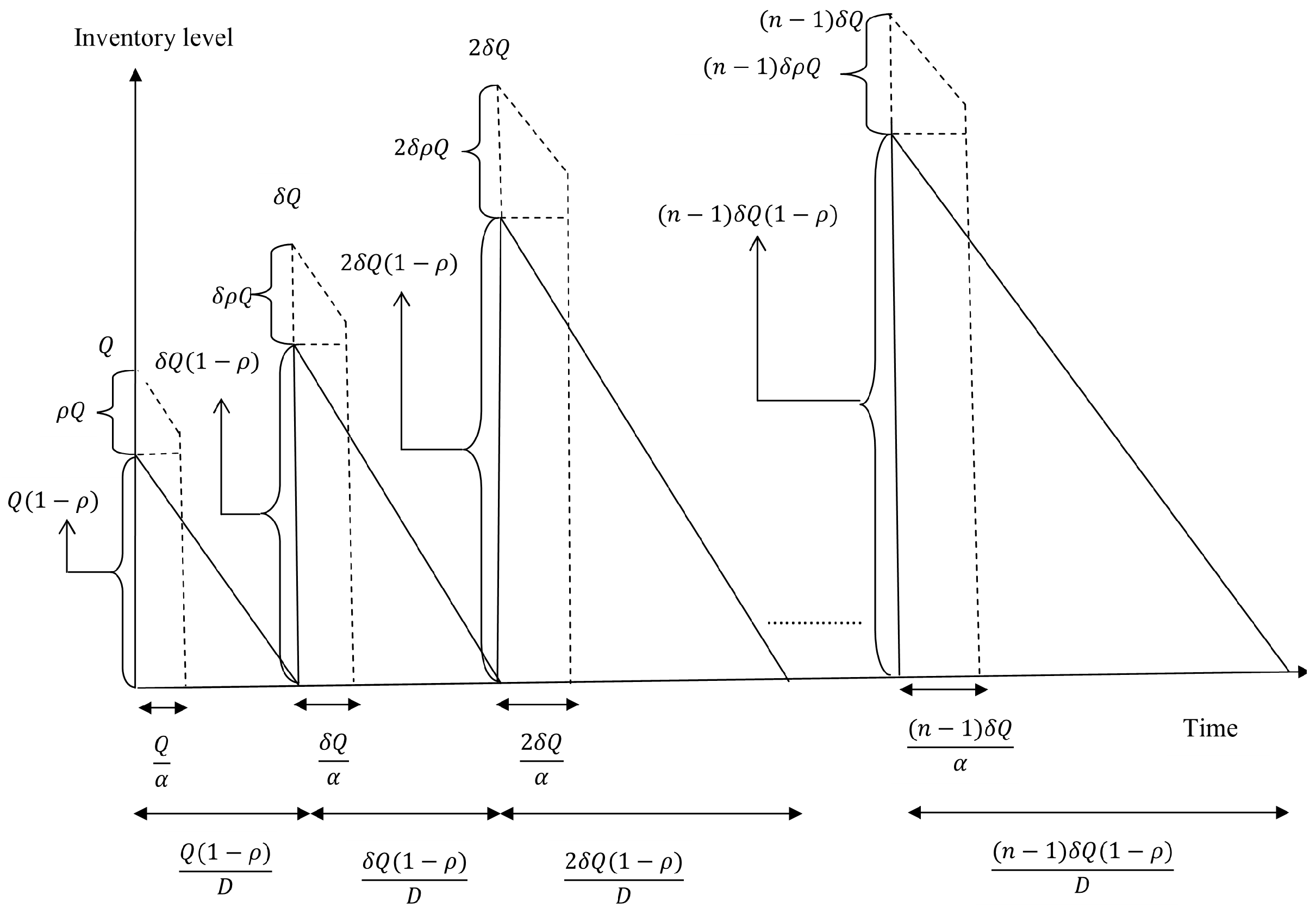
Initially, buyer orders some products with ordering cost $A_b$. Vendor produces items with a fixed production rate P and initial setup cost of vendor is $V_0$. Vendor uses some investments I for reducing that setup cost and sends first lots of each batch i.e., Q units with some fixed transportation cost F as well as variable transportation cost $V_t$. Vendor continues the whole delivery products in n times. Initially, first shipment lot size per batch is Q. It is assumed that the increasing rate of delivery lots as δ. Therefore, vendor’s second shipment lot size is $\delta Q$. Vendor transports third shipment lot size as $2\delta Q$. In this way, it can be found that the number of quantity transferred to buyer on $yth$ delivery is $(y-1)\delta Q$, $y>1$. Throughout unequal delivery goods, vendor pays fixed carbon-emission cost $C_v$ and also variable carbon-emission cost $V_v$. While that delivery lots placed to buyer, then buyer performs an inspecting procedure to check the quality of the received lots. Buyer incurs two types of inspection costs, which are variable inspection cost $V_i$ and unit inspection cost $U_i$, where screening rate is α. The rate of imperfect item is ρ in each lot. When the inspection has been completed, both perfect and imperfect items are separated. For holding perfect items, buyer incurs some cost $h_{b_1}$. In addition, buyer’s holding cost for imperfect items is $h_{b_2}$. While next produced lot comes to buyer from vendor, buyer sent back all imperfect products of previous lot to vendor for reworking. In this case, it is assumed that buyer has not pay any delivery cost for shifting imperfect products to vendor.

3.1. Vendor’s Mathematical Model

Vendor sends ordering lots in n times in each production cycle by using single-setup-multi-delivery (SSMD) policy.

One can measured the total production batch, which shipped to buyer from vendor is formulated by adding the whole delivery lots

$$Q+\delta Q+2\delta Q+...+(n-1)\delta Q=Q+\frac{\delta Qn(n-1)}{2}.$$

Total production cycle is obtained by splitting the demand with total production batch.

$$\frac{D}{Q+\delta \frac{n(n-1)}{2}Q}=\frac{2D}{2Q+Q\delta n(n-1)}.$$

As the number of total production cycle is $\frac{D}{Q+\delta \frac{n(n-1)}{2}Q}$=$\frac{2D}{2Q+Q\delta n(n-1)}$, setup cost is $V_0$, and investment to minimize setup cost is I.

Vendor’s total setup cost is $V_0{e}^{-\kappa I}\left(\frac{2D}{2Q+\delta n(n-1)Q}\right)$.

Vendor’s total investment cost is $\frac{2DI}{2Q+\delta n(n-1)Q}$.

At the beginning, while the production batch is around to commence, systems’s total stock is starting with zero. On the other hand, buyer has sufficient stock to meet satisfy the demand before the first delivery lot comes. Buyer stock is $\frac{DQ}{P}$. The total stock inclined at a rate of $P-D$ while producing the batch quantity of $Q+\frac{\delta Qn(n-1)}{2}$ with the rate P and arrives the maximum level of $\frac{DQ}{P}+(P-D)\left(\frac{2Q+\delta n(n-1)Q}{2P}\right)$ when manufacturing of batch completed.

Therefore, system’s average total stock is

$$\frac{DQ}{P}+(P-D)\left(\frac{2Q+\delta n(n-1)Q}{4P}\right).$$

On the other hand, average buyer stock consists of perfect as well as imperfect products.

i.e., average buyer stock is $\left(\frac{Q{(1-\rho )}^2[2+\delta n(n-1)]}{4}\right)+\left(\frac{Q\rho D[2+\delta n(n-1\left)\right]}{2\alpha }\right)$.

Then average vendor stock can be measured by deducting system’s average total stock less the average buyer stock.

Hence, average vendor stock is

$$\frac{DQ}{P}+(P-D)\left(\frac{2Q+\delta n(n-1)Q}{4P}\right)-\left(\frac{Q{(1-\rho )}^2[2+\delta n(n-1)]}{4}\right)-\left(\frac{Q\rho D[2+\delta n(n-1\left)\right]}{2\alpha }\right).$$

Vendor’s total holding cost is

$$T{h}_v=H_v\left[(P-D)\left(\frac{2Q+\delta n(n-1)Q}{4P}\right)-\left(\frac{Q{(1-\rho )}^2[2+\delta n(n-1)]}{4}\right)-\left(\frac{Q\rho D[2+\delta n(n-1\left)\right]}{2\alpha }\right)+\frac{DQ}{P}\right].$$

Vendor’s total transportation cost is measured by adding fixed and variable transportation costs which is

$$T{r}_v=\frac{2nFD}{2Q+\delta n(n-1)Q}+V_t\rho D.$$

Vendor’s total carbon-emission cost can be obtained by calculating fixed and variable carbon-emission costs.

As the number of total production cycle is $\frac{2D}{2Q+Q\delta n(n-1)}$, vendor’s fixed carbon-emission cost per delivery is $C_v$, and number of delivery lots of each batch per production is n.

Therefore, vendor’s fixed carbon-emission cost is $\frac{2n{C}_{v}D}{2Q+\delta n(n-1)Q}$.

Likewise, for defective rate ρ, demand D, and vendor’s variable carbon-emission cost per unit $V_v$.

The vendor’s variable carbon-emission cost is given by $V_v\rho D$.

Hence, the vendor’s total carbon-emission cost is $C{E}_v=\frac{2n{C}_{v}D}{2Q+\delta n(n-1)Q}+V_v\rho D$.

Total rework cost for the vendor is $R_v\rho D$.

Then, the vendor’s total inventory cost can be obtained by summing setup cost, holding cost, investment cost to minimize setup cost, fixed and variable transportation cost, fixed as well as variable carbon-emission cost, and rework cost.

$$\begin{array}{cc}T{C}_v(n,Q,\delta ,I)\hfill & =\frac{2D}{2Q+\delta n(n-1)Q}(V_0{e}^{-\kappa I}+n{C}_v+I+nF)+\rho D(V_v+V_t+R_v)\hfill \\ & +h_{v}Q\left[\frac{D}{P}+(2+\delta n(n-1))\left(\frac{(P-D)}{4P}-\frac{{(1-\rho )}^2}{4}-\frac{\rho D}{2\alpha }\right)\right]\hfill \end{array}$$

3.2. Buyer’s Mathematical Model

The buyer incurs total ordering cost for whole production cycle is $A_b\left(\frac{2D}{2Q+\delta n(n-1)Q}\right)$.

During the inspecting process, the buyer considers two types of inspection costs i.e., unit as well as variable inspection cost.

Total inspection cost for the buyer is $D{U}_i+\frac{2n{V}_{i}D}{2Q+\delta n(n-1)Q}$.

The total number of perfect products for whole production cycle is observed from the area of the triangle given in Figure 1, which is obtained as

$$\frac{Q(1-\rho )}{2}\frac{(1-\rho )Q}{D}+\frac{\delta Q(1-\rho )}{2}\frac{\delta (1-\rho )Q}{D}+...+\frac{(n-1)\delta Q(1-\rho )}{2}\frac{(n-1)\delta (1-\rho )Q}{D}=\frac{1}{2}\frac{Q^2{(1-\rho )}^2}{D}\left[1+\frac{{\delta }^{2}n(n-1)(2n-1)}{6}\right].$$

Hence, the buyer’s total holding cost for perfect products $T{h}_{b_1}$ is obtained by multiplying all perfect products with production cycle i.e.,

$$T{h}_{b_1}=h_{b_1}\left[\frac{1}{2}\frac{Q^2{(1-\rho )}^2}{D}\left(1+\frac{{\delta }^{2}n(n-1)(2n-1)}{6}\right)\right]\left[\frac{2D}{2Q+\delta Qn(n-1)}\right]=h_{b_1}\left[\left(\frac{Q{(1-\rho )}^2}{2+\delta n(n-1)}\right)\left(1+\frac{{\delta }^{2}n(n-1)(2n-1)}{6}\right)\right].$$

The total quantity of imperfect products is calculated by the parallelogram shown in Figure 1.

$$Q\rho \frac{Q}{\alpha }+\delta Q\rho \frac{\delta Q}{\alpha }+...+\delta (n-1)Q\rho \frac{(n-1)\delta Q}{\alpha }=\frac{Q^2\rho }{\alpha }\left(1+\frac{{\delta }^{2}n(n-1)(2n-1)}{6}\right)$$

The buyer’s total holding cost for imperfect products $T{h}_{b_2}$ is given by multiplying total imperfect products with production cycle.

$$T{h}_{b_2}=h_{b_2}\left[\frac{Q^2\rho }{\alpha }\left(1+\frac{{\delta }^{2}n(n-1)(2n-1)}{6}\right)\right]\left[\frac{2D}{2Q+\delta Qn(n-1)}\right]=h_{b_2}\left[\frac{2DQ\rho }{\alpha (2+\delta n(n-1\left)\right)}\left(1+\frac{{\delta }^{2}n(n-1)(2n-1)}{6}\right)\right]$$

Therefore, the buyer’s total inventory cost can be determined by adding ordering cost, inspection cost, holding cost of perfect products items, and imperfect products.

$$T{C}_b(n,Q,\delta )=\frac{2D}{2Q+\delta n(n-1)Q}(A_b+n{V}_i)+D{U}_i+\left({(1-\rho )}^2{h}_{b_1}+\frac{2D\rho }{\alpha }{h}_{b_2}\right)\left(1+\frac{{\delta }^{2}n(n-1)(2n-1)}{6}\right)\frac{Q}{(2+\delta n(n-1\left)\right)}$$

Hence, the vendor-buyer system’s joint total cost $JT{C}_{vb}$ is given by

$$\begin{array}{ccc}\hfill JT{C}_{vb}(n,Q,\delta ,I)& =& \frac{2D}{2Q+\delta Qn(n-1)}(V_0{e}^{-\kappa I}+n{C}_v+I+nF+A_b+n{V}_i)+D{U}_i+\rho D(V_v+V_t\hfill \\ & +& R_v)+h_v\left[\left(\frac{(P-D)}{2P}-\frac{{(1-\rho )}^2}{2}-\frac{\rho D}{\alpha }\right)\left(\frac{2Q+\delta n(n-1)Q}{2}\right)+\frac{DQ}{P}\right]\hfill \\ & +& \left(\frac{2D\rho }{\alpha }{h}_{b_2}+{(1-\rho )}^2{h}_{b_1}\right)\frac{Q}{2+\delta n(n-1)}\left(1+\frac{{\delta }^{2}n(n-1)(2n-1)}{6}\right).\hfill \end{array}$$

The necessary conditions to minimize the vendor-buyer system’s joint total cost $JT{C}_{vb}$ are $\frac{\partial JT{C}_{vb}}{\partial I}=0$, $\frac{\partial JT{C}_{vb}}{\partial Q}=0$, $\frac{\partial JT{C}_{vb}}{\partial \delta }=0$, and $\frac{\partial JT{C}_{vb}}{\partial n}=0$.

The first order partial derivative of the vendor-buyer system’s joint total cost $JT{C}_{vb}$ with respect to number of delivery lots of each batch per production n (by considering number of shipment as continuous variable) is given by

$$\begin{array}{ccc}\hfill \frac{\partial JT{C}_{vb}}{\partial n}& =& \frac{2D{R}_3}{2Q+\delta Qn(n-1)}-\frac{2DQ\delta (2n-1)}{{(2Q+\delta Qn(n-1))}^2}(V_0{e}^{-\kappa I}+n{R}_3+I+A_b)+\frac{h_v{R}_1\delta Q(2n-1)}{2}\hfill \\ & +& R_2\left[\frac{(2n^3-3n^2+n)Q}{6(2+\delta n(n-1\left)\right)}-\left(\frac{{\delta }^{2}n(n-1)(2n-1)}{6}+1\right)\frac{Q\delta (2n-1)}{2+\delta n(n-1)}\right].\hfill \end{array}$$

By calculating $\beta \left(n^{*}\right)=0$, where $\beta \left(n\right)=\frac{\partial JT{C}_{vb}}{\partial n}$, the optimal value of n (say $n^{*}$) is obtained.

See Appendix A for the values of $R_1$, $R_2$, and $R_3$. The first order partial derivative of vendor-buyer system’s joint total cost $JT{C}_{vb}$ with respect to first shipment lot size per batch throughout the production Q is

$$\begin{array}{ccc}\hfill \frac{\partial JT{C}_{vb}}{\partial Q}& =& \frac{2D}{Q^2(2+\delta n(n-1))}(V_0{e}^{-\kappa I}+n{C}_v+I+nF+A_b+n{V}_i)-h_v\left[R_1\right(\frac{(2+\delta n(n-1\left)\right)}{2}\hfill \\ & +& \frac{D}{P}\left)\right]+\frac{R_2}{2+\delta n(n-1)}\left(\frac{{\delta }^{2}n(n-1)(2n-1)}{6}+1\right).\hfill \end{array}$$

The optimum value $Q^{*}$ is given by

$$Q^{*}=\sqrt{\frac{2D(V_0{e}^{-\kappa I}+n{R}_3+I+A_b)}{\left[h_v(2+\delta n(n-1))\left(R_1\frac{(2+\delta n(n-1\left)\right)}{2}+\frac{D}{P}\right)+\left(1+\frac{{\delta }^{2}n(n-1)(2n-1)}{6}\right)R_2\right]}}.$$

Now, the first order partial derivative of the vendor-buyer system’s joint total cost $JT{C}_{vb}$ with respect to investment for setup cost reduction per production run I is

$$\frac{\partial JT{C}_{vb}}{\partial I}=\frac{2D}{2Q+\delta n(n-1)Q}(1-V_0\kappa e^{-\kappa I}).$$

From the equation $\frac{\partial JT{C}_{vb}}{\partial I}=0$, the optimal value of I (say $I^{*}$) will be $I^{*}=\frac{1}{\kappa }ln\left(V_0\kappa \right).$

Again, the first order partial derivative of vendor-buyer system’s joint total cost $JT{C}_{vb}$ regarding rate of increasing delivery lots δ is

$$\begin{array}{ccc}\hfill \frac{\partial JT{C}_{vb}}{\partial \delta }& =& -\frac{2DQn(n-1)}{{2Q+\delta Qn(n-1)}^2}(V_0{e}^{-\kappa I}+n{R}_3+I+A_b)+\frac{h_v{R}_{1}n(n-1)Q}{2}\hfill \\ & +& R_2\left[\frac{\delta (2n^3-3n^2+n)Q}{6(2+\delta n(n-1\left)\right)}-\frac{Qn(n-1)}{{(2+\delta n(n-1))}^2}\left(\frac{{\delta }^{2}n(n-1)(2n-1)}{6}+1\right)\right].\hfill \end{array}$$

Similarly as n, I, and Q, in this case the optimal value of δ (say ${\delta }^{*}$) can be calculated if it satisfies $\xi \left({\delta }^{*}\right)=0$, where $\xi \left(\delta \right)=\frac{\partial JT{C}_{vb}}{\partial \delta }$.

Now, Hessian matrix at the optimal values, i.e., $n^{*}$, $Q^{*}$, ${\delta }^{*}$, and $I^{*}$ are calculated as

$$\begin{array}{c}\hfill H_{ii}=\left[\begin{array}{c}\frac{{\partial }^{2}JT{C}_{vb}(·)}{\partial {I^{*}}^2}\frac{{\partial }^{2}JT{C}_{vb}(·)}{\partial I^{*}\partial Q^{*}}\frac{{\partial }^{2}JT{C}_{vb}(·)}{\partial I^{*}\partial n^{*}}\frac{{\partial }^{2}JT{C}_{vb}(·)}{\partial I^{*}\partial {\delta }^{*}}\\ \frac{{\partial }^{2}JT{C}_{vb}(·)}{\partial Q^{*}\partial I^{*}}\frac{{\partial }^{2}JT{C}_{vb}(·)}{\partial {Q^{*}}^2}\frac{{\partial }^{2}JT{C}_{vb}(·)}{\partial Q^{*}\partial n^{*}}\frac{{\partial }^{2}JT{C}_{vb}(·)}{\partial Q^{*}\partial {\delta }^{*}}\\ \frac{{\partial }^{2}JT{C}_{vb}(·)}{\partial n^{*}\partial I^{*}}\frac{{\partial }^{2}JT{C}_{vb}(·)}{\partial n^{*}\partial Q^{*}}\frac{{\partial }^{2}JT{C}_{vb}(·)}{\partial {n^{*}}^2}\frac{{\partial }^{2}JT{C}_{vb}(·)}{\partial n^{*}\partial {\delta }^{*}}\\ \frac{{\partial }^{2}JT{C}_{vb}(·)}{\partial {\delta }^{*}\partial I^{*}}\frac{{\partial }^{2}JT{C}_{vb}(·)}{\partial {\delta }^{*}\partial Q^{*}}\frac{{\partial }^{2}JT{C}_{vb}(·)}{\partial {\delta }^{*}\partial n^{*}}\frac{{\partial }^{2}JT{C}_{vb}(·)}{\partial {{\delta }^{*}}^2}\end{array}\right]\end{array}$$

where $JT{C}_{vb}(·)=JTC(n^{*},Q^{*},{\delta }^{*},I^{*})$.

The optimal values $n^{*}$, $I^{*}$, $Q^{*}$, and ${\delta }^{*}$ for minimize vendor-buyer system’s joint total cost $JT{C}_{vb}$ must fulfil the conditions that all principal minors of Hessian matrix $H_{ii}$ are positive. As the expressions of second order partial derivatives of $JT{C}_{vb}$ are non-linear (see Appendix B), thus each principal minors of the Hessian matrix $H_{ii}$ are extremely non-linear. Hence, those conditions to minimize vendor-buyer system’s joint total cost $JT{C}_{vb}$ are determined by considering some numerical examples and graphical representations.

4. Solution Methodology

Within the supply chain, it is not always possible that players of the chain are with equal power always. Sometime, retailer is more powerful like different shopping malls, sometimes manufacturer are more powerful like Microsoft. Then, it cannot be considered only joint total cost. It is required to assume someone as leader and someone as follower based on the more dominating nature of the players. For this general model, each one is considered as leader and each one is considered as follower and optimize the cost to check which is the best possible combination.

Case 1.

(While buyer as leader and vendor as follower).

Using Stackelberg approach, vendor’s cost function is optimized with respect to four decision variables namely n, Q, δ, and I.

Vendor’s cost function is

$$\begin{array}{ccc}\hfill T{C}_v(n,Q,\delta ,I)& =& \frac{2D}{2Q+\delta n(n-1)Q}(V_0{e}^{-\kappa I}+n{C}_v+I+nF)+\rho D(V_v+V_t+R_v)\hfill \\ & +& h_{v}Q\left[\frac{D}{P}+(2+\delta n(n-1))\left(\frac{(P-D)}{4P}-\frac{{(1-\rho )}^2}{4}-\frac{\rho D}{2\alpha }\right)\right].\hfill \end{array}$$

The first order partial derivative of $T{C}_v$ with respect to I is given by

$$\begin{array}{ccc}\hfill \frac{\partial T{C}_v}{\partial I}& =& \frac{2D}{2Q+\delta n(n-1)Q}(1-V_0\kappa e^{-\kappa I}).\hfill \end{array}$$

The optimum value of I (say $I^{*}$) is

$$\begin{array}{ccc}\hfill I^{*}& =& \frac{1}{\kappa }ln\left(V_0\kappa \right).\hfill \end{array}$$

Equating the first order partial derivative of $T{C}_v$ with respect to Q to zero, which is

$$\begin{array}{ccc}\hfill \frac{\partial T{C}_v}{\partial Q}& =& \frac{2D}{Q^2(2+\delta n(n-1))}(V_0{e}^{-\kappa I}+n{C}_v+I+nF)-D\rho (V_v+V_t+R_v)\hfill \\ & -& h_v\left(\frac{D}{P}+\frac{(2+\delta n(n-1\left)\right)}{2}{R}_1\right)=0.\hfill \end{array}$$

The optimum value $Q^{*}$ is calculated as follows:

$$\begin{array}{ccc}\hfill Q^{*}& =& \sqrt{\frac{2D(V_0{e}^{-\kappa I}+n{C}_v+I+nF)}{\left(R_4+h_v\left(\frac{D}{P}+\frac{(2+\delta n(n-1\left)\right)}{2}{R}_1\right)\right)(2+\delta n(n-1))}}.\hfill \end{array}$$

(See Appendix A for the values of $R_4$.)

${\delta }^{*}$ will be evaluated from the following equation, which is the first order partial derivative of $T{C}_v$ with respect to δ.

$$\begin{array}{ccc}\hfill \frac{\partial T{C}_v}{\partial \delta }& =& \frac{h_{v}Qn(n-1)R_1}{4DQn(n-1)(V_0{e}^{-\kappa I}+n{C}_v+I+nF)}-\frac{1}{{(2Q+\delta Qn(n-1))}^2}\hfill \end{array}$$

Therefore,

$$\begin{array}{ccc}\hfill {\delta }^{*}& =& \frac{1}{Qn(n-1)}\sqrt{\frac{2DQn(n-1)(V_0{e}^{-\kappa I}+n{C}_v+I+nF)}{h_{v}Qn(n-1)\frac{R_1}{2}}}-2Q.\hfill \end{array}$$

Finally, the first order derivative of $T{C}_v$ with respect to n is as follows:

$$\begin{array}{ccc}\hfill \frac{\partial T{C}_v}{\partial n}& =& \frac{2D}{2Q+\delta Qn(n-1)}\left(\frac{\delta Q(1-2n)(V_0{e}^{-\kappa I}+n{C}_v+I+nF)}{2Q+\delta n(n-1)}+(C_v+F)\right)\hfill \\ & +& h_{v}Q\delta (2n-1)\frac{R_1}{2}.\hfill \end{array}$$

Therefore, the optimum value of n (say $n^{*}$) will be obtained by equating $\varphi \left(n^{*}\right)=\frac{\partial T{C}_v}{\partial n}=0$.

Substituting all optimum values, i.e., $I^{*}$, $Q^{*}$, $n^{*}$, and ${\delta }^{*}$ into the buyer’s cost function, the optimized buyer’s cost function can be obtained as

$$\begin{array}{ccc}\hfill T{C}_b(n^{*},Q^{*},{\delta }^{*})& =& \frac{2D}{2Q^{*}+{\delta }^{*}{n}^{*}(n^{*}-1)Q^{*}}(A_b+n^{*}{V}_i)+D{U}_i+({(1-\rho )}^2{h}_{b_1}\hfill \\ & +& \frac{2D\rho }{\alpha }{h}_{b_2})\left(1+\frac{{{\delta }^{*}}^2{n}^{*}(n^{*}-1)(2n^{*}-1)}{6}\right)\frac{Q^{*}}{(2+{\delta }^{*}{n}^{*}(n^{*}-1))}.\hfill \end{array}$$

Case 2.

(While vendor as leader and buyer as follower).

In this case, buyer’s cost function is optimized with respect to three decision variables namely n, Q, and δ.

Buyer’s cost function is

$$\begin{array}{ccc}\hfill T{C}_b(n,Q,\delta )& =& \frac{2D}{2Q+\delta n(n-1)Q}(A_b+n{V}_i)+D{U}_i+({(1-\rho )}^2{h}_{b_1}\hfill \\ & +& \frac{2D\rho }{\alpha }{h}_{b_2})\left(1+\frac{{\delta }^{2}n(n-1)(2n-1)}{6}\right)\frac{Q}{(2+\delta n(n-1\left)\right)}.\hfill \end{array}$$

The first order partial derivative of $T{C}_b$ with respect to Q is given by

$$\begin{array}{ccc}\hfill \frac{\partial T{C}_b}{\partial Q}& =& \frac{2D(A_b+n{V}_i)}{Q^2(2+\delta n(n-1))}-\frac{D{U}_i{R}_2}{2+\delta n(n-1)}\left(1+\frac{{\delta }^{2}n(n-1)(2n-1)}{6}\right).\hfill \end{array}$$

The optimum value of Q (say $Q^{*}$) is

$$\begin{array}{ccc}\hfill Q^{*}& =& \sqrt{\frac{2(A_b+n{V}_i)}{U_i{R}_2\left(1+\frac{{\delta }^{2}n(n-1)(2n-1)}{6}\right)}}.\hfill \end{array}$$

The optimal value of δ (say ${\delta }^{*}$) will be found from the equation $\psi \left({\delta }^{*}\right)=0$,

where

$$\begin{array}{ccc}\hfill \psi \left(\delta \right)=\frac{\partial T{C}_b}{\partial \delta }& =& D{U}_i\left(\frac{Qn(n-1)R_2}{(2+\delta n(n-1\left)\right)}\right(\frac{\delta (2n-1)}{3}-\frac{1}{2+\delta n(n-1)}(1\hfill \\ & +& \frac{{\delta }^{2}n(n-1)(2n-1)}{6}\left)\right))-\frac{2Dn(n-1)(A_b+n{V}_i)}{Q{(2+\delta n(n-1))}^2}.\hfill \end{array}$$

Putting all optimum values, i.e., $Q^{*}$, ${\delta }^{*}$, and $n^{*}$ into the vendor’s cost function, the optimized vendor’s cost function can be obtained as

$$\begin{array}{ccc}\hfill T{C}_v(n^{*},Q^{*},{\delta }^{*},I)& =& \frac{2D}{2Q^{*}+{\delta }^{*}{n}^{*}(n^{*}-1)Q^{*}}(V_0{e}^{-\kappa I}+n^{*}{C}_v+I+n^{*}F)+\rho D(V_v+V_t\hfill \\ & +& R_v)+h_v{Q}^{*}\left[\frac{D}{P}+({\delta }^{*}{n}^{*}(n^{*}-1)+2)\left(\frac{(P-D)}{4P}-\frac{{(1-\rho )}^2}{4}-\frac{\rho D}{2\alpha }\right)\right].\hfill \end{array}$$

The optimal value of I (say $I^{*}$) will be determined from the above equation as

$$\begin{array}{c}\hfill I^{*}=\frac{1}{\kappa }ln\left(V_0\kappa \right).\end{array}$$

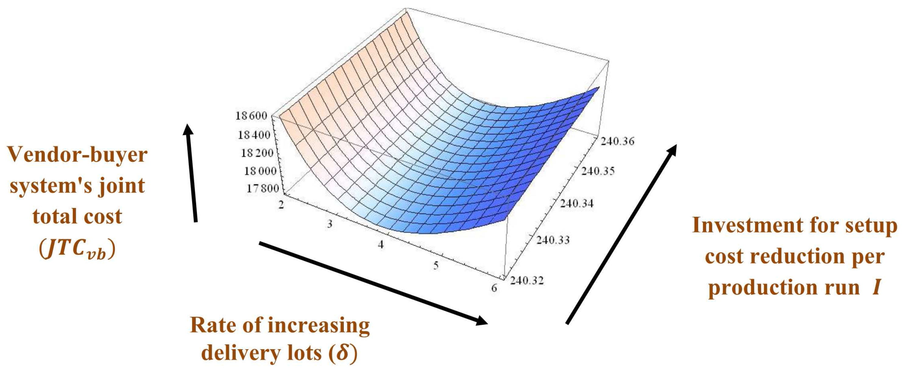
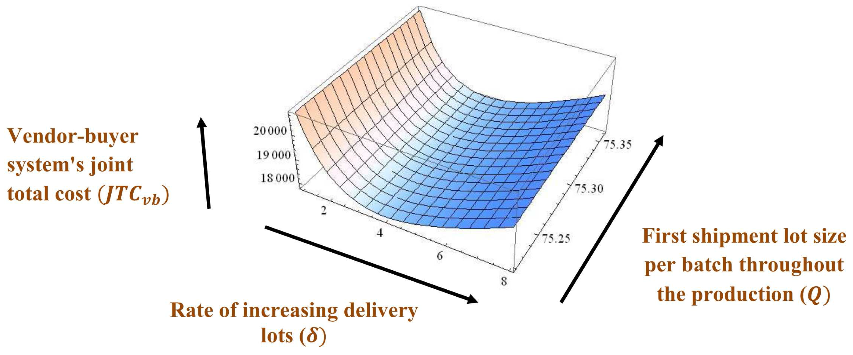
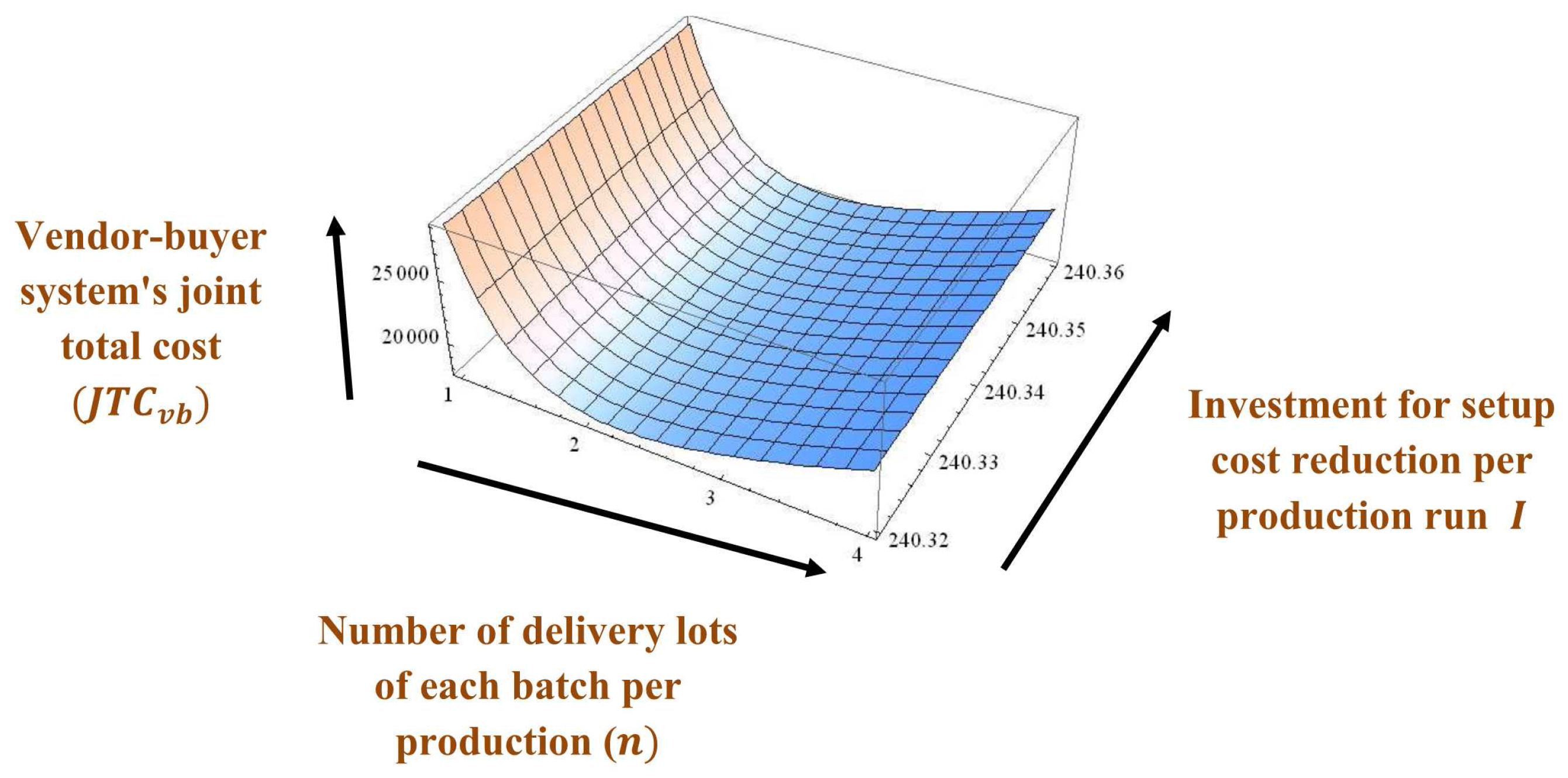
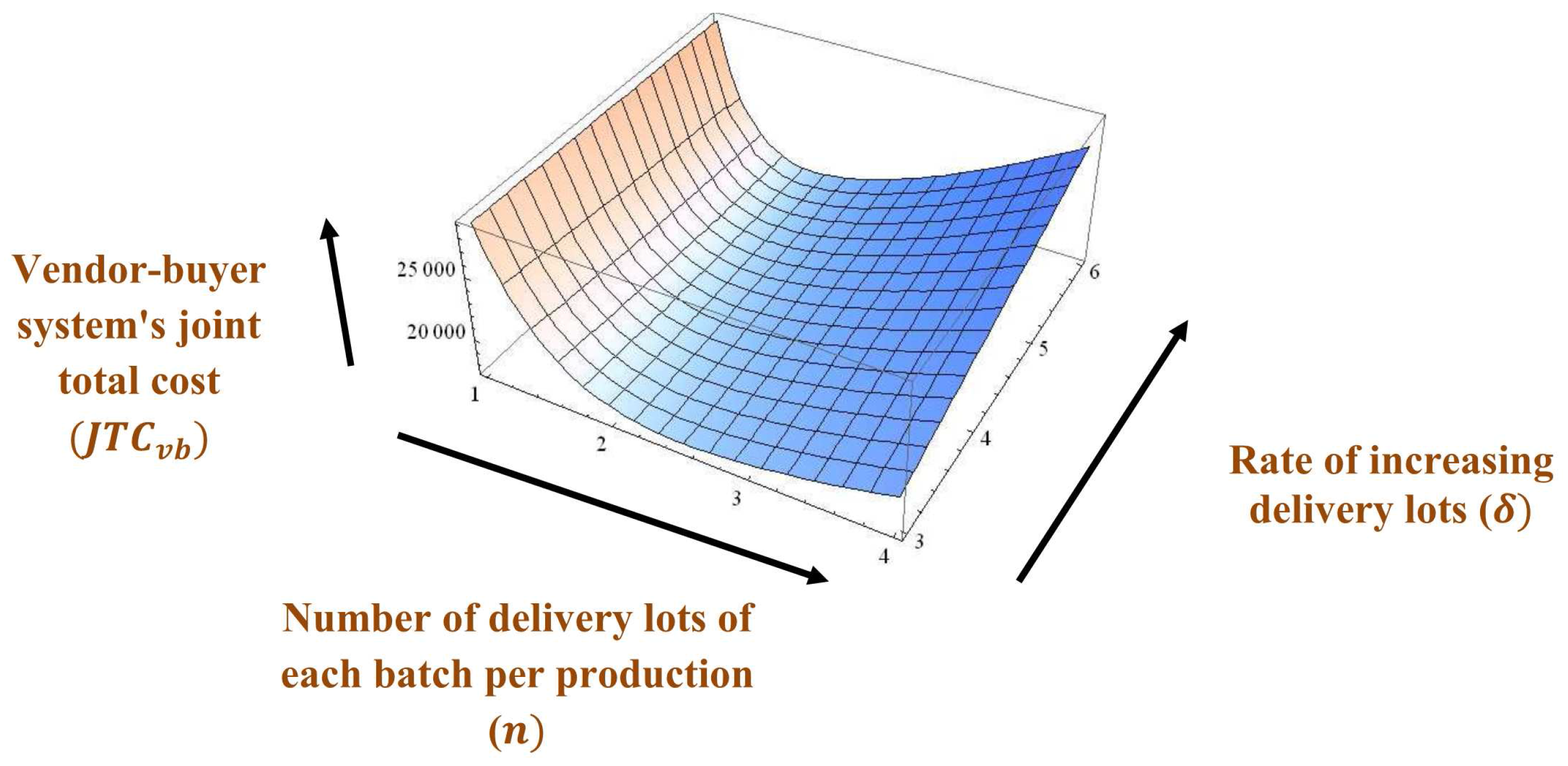
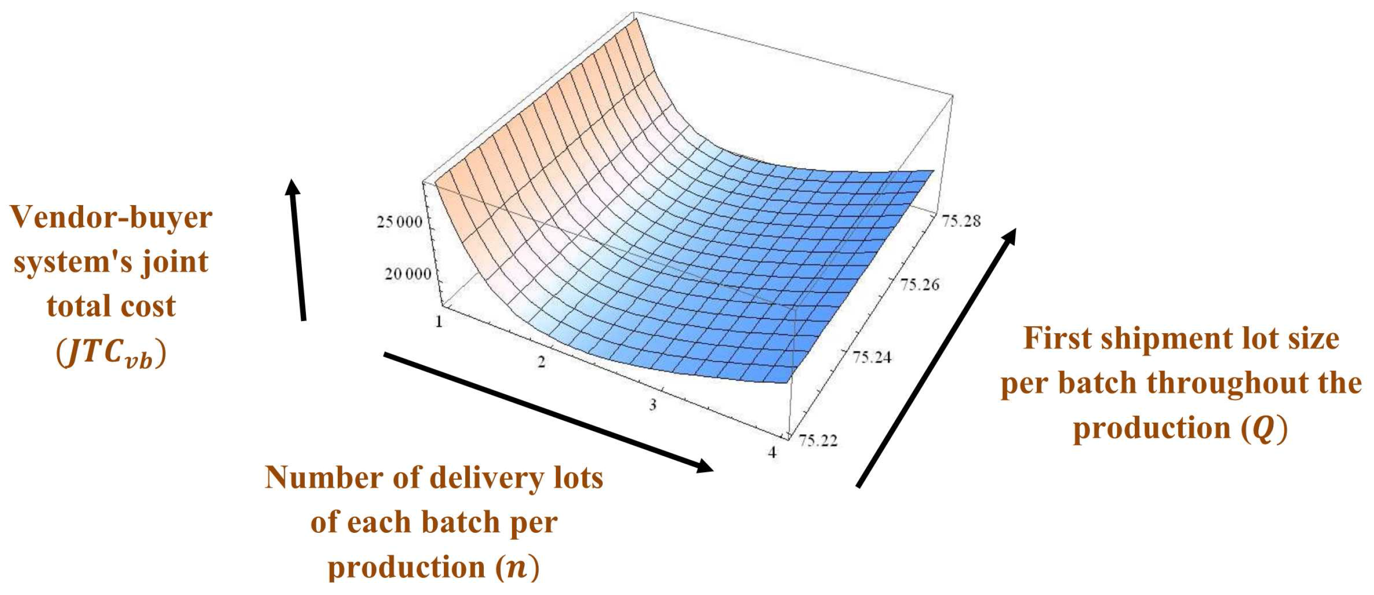
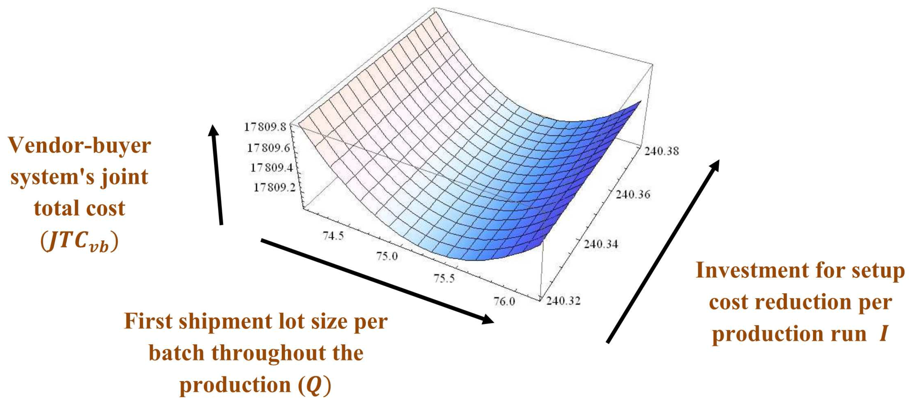
5. Numerical Example without Stackelberg Approach

Example 1.

The values of parameters are considered by using the numerical data from Sarkar [8], Huang et al. [22], Sarkar et al. [44], and Sarkar et al. [45] as

$D=1000$ units/year, $P=4000$ units/year, $A_b=\$300$/order, $A_3=\$100$/shipment, $C_v=\$5$/delivery, $F=\$0.2$/shipment, $V_t=\$0.1$/unit, $V_i=\$1$/delivery, $U_i=\$0.2$/unit item inspected, $R_v=\$15$/unit, $\rho =0.55$, $V_v=\$5$/unit, $h_{b_1}=\$35$/unit/year, $h_{b_2}=\$30$/unit/year, $h_v=\$20$/unit/year, $\alpha =3500$ units/year, $\kappa =0.0014$, and $V_0=\$1000$/setup. Therefore, after applying the investment vendor’s setup cost becomes $V_s=\$714.28$/setup.

Hence, the vendor-buyer system’s joint total cost $JT{C}_{vb}=\$17809$, first shipment lot size per batch throughout the production $Q^{*}=75$ units, rate of increasing delivery lots ${\delta }^{*}=4$ unit/year, and number of delivery lots of each batch per production $n^{*}=2$, and investment for setup cost reduction per production run $I^{*}=\$240.34$/production run, see Figure 2, Figure 3, Figure 4, Figure 5, Figure 6 and Figure 7 for graphical representations of the total cost with optimum values.

5.1. Sensitivity Analysis

The sensitivity analysis conducted for the key parameters.

This section illustrates sensitivity analysis, which shows (

Table 3. Sensitivity analysis of key parameters of the model with equal power.

Parameters	Changes (in %)	${\mathit{JTC}}_{\mathit{vb}}$	Parameters	Changes (in %)	${\mathit{JTC}}_{\mathit{vb}}$
	−50%	−0.09		−50%	−0.07
	−25%	−0.04		−25%	−0.04
$V_i$	+25%	0.04	$C_v$	+25%	0.04
	+50%	0.09		+50%	0.07
	−50%	−0.06		−50%	−2.31
	−25%	−0.03		−25%	−1.14
$U_i$	+25%	0.03	$A_b$	+25%	1.10
	+50%	0.06		+50%	2.17
	−50%	−0.003		−50%	−3.70
	−25%	−0.001		−25%	−1.80
F	+25%	0.001	$V_t$	+25%	1.72
	+50%	0.003		+50%	3.37
	−50%	−2.64		−50%	−29.83
	−25%	−1.30		−25%	−14.98
$h_{b_1}$	+25%	1.25	ρ	+25%	15.13
	+50%	2.46		+50%	30.41
	−50%	−3.55		−50%	−3.70
	−25%	−1.73		−25%	−1.80
$h_{b_2}$	+25%	1.66	$h_v$	+25%	1.72
	+50%	3.25		+50%	3.37

) the impact of each parameters which are $V_i$, $U_i$, F, $V_t$, ρ, $h_v$, $C_v$, $h_{b_1}$, $h_{b_2}$, and $A_b$, respectively on vendor-buyer system’s joint total cost $JT{C}_{vb}$.

•

The vendor-buyer system’s joint total cost $JT{C}_{vb}$ increases while unit and variable inspection costs i.e., $U_i$ and $V_i$ increase. On the other hand, if unit transportation cost F and variable transportation cost $V_t$ are increased, then vendor-buyer system’s joint total cost $JT{C}_{vb}$ is also increased.

•

If defective rate ρ, vendor’s holding cost $h_v$, and vendor’s fixed carbon-emission cost $C_v$ increase, then vendor-buyer system’s joint total cost $JT{C}_{vb}$ also increases.

•

Increasing values in buyer’s holding cost for perfect items $h_{b_1}$, holding cost for imperfect items $h_{b_2}$, and buyer’s ordering cost $A_b$ imply that vendor-buyer system’s joint total cost $JT{C}_{vb}$ is increased. It is found that the negative percentage changes for these three parameters $h_{b_1}$, $h_{b_2}$, $A_b$ are much more sensitive than the positive percentage changes.

5.2. Numerical Example by Using Stackelberg Approach

Case 1.

Buyer as leader and vendor as follower

Example 2.

$D=1000$ units/year, $P=4000$ units/year, $A_b=\$300$/order, $A_3=\$100$/shipment, $C_v=\$5$/delivery, $F=\$0.2$/shipment, $V_t=\$0.1$/unit, $V_i=\$1$/delivery, $U_i=\$0.2$/unit item inspected, $R_v=\$15$/unit, $\rho =0.55$, $V_v=\$5$/unit, $h_{b_1}=\$35$/unit/year, $h_{b_2}=\$30$/unit/year, $h_v=\$20$/unit/year, $\alpha =3500$ units/year, $\kappa =0.0014$, and $V_0=\$1000$/setup.

Hence, vendor-buyer system’s joint total cost $JT{C}_{vb}=\$17,131.36$, first shipment lot size per batch throughout the production $Q^{*}=58$ units, rate of increasing delivery lots ${\delta }^{*}=3$ unit/year, and number of delivery lots of each batch per production $n^{*}=3$, and investment for setup cost reduction per production run $I^{*}=\$240.34$/production run.

The results, which are obtained in our paper, are compared with the paper of Sarkar et al. [44]. In Sarkar et al. [44], vendor-buyer system’s joint total cost is $JT{C}_{vb}=\$24,045.8$ which is larger in compared to this model. Therefore, this proposed model formulates more appropriate results than Sarkar et al. [44] by incorporating the Stackelberg approach.

This section discusses the effect on the total cost for buyer $T{C}_b$ by changing several parameters such as $A_b$, $V_i$, $U_i$, and $h_{b_1}$, respectively (see

Table 4. Sensitivity analysis for buyer’s cost.

Parameters	Changes (in %)	${\mathit{TC}}_{\mathit{b}}$	Parameters	Changes (in %)	${\mathit{TC}}_{\mathit{b}}$
	−50%	−9.28		−50%	−0.36
	−25%	−4.64		−25%	−0.18
$A_b$	+25%	4.64	$U_i$	+25%	0.18
	+50%	9.28		+50%	0.36
	−50%	−0.09		−50%	−17.28
	−25%	−0.05		−25%	−8.64
$V_i$	+25%	0.05	$h_{b_1}$	+25%	8.64
	+50%	0.09		+50%	17.28

).

•

For the parameter $A_b$, which is buyer’s ordering cost, negative and positive percentage changes are similar. If the value of the parameter $A_b$ increases that indicates buyer’s total cost $T{C}_b$ also increases.

•

It is observed if unit inspection cost $U_i$ and variable inspection cost $V_i$ are increased, then buyer’s total cost $T{C}_b$ also increases.

•

When buyer’s holding cost for perfect items, i.e., $h_{b_1}$ increases, then buyer’s total cost $T{C}_b$ is increased. Both negative percentage change and positive percentage changes are similar for this parameter.

This section allows sensitivity analysis for evaluating the effect of several parameters such as $V_v$, $h_v$, F, and $C_v$, respectively on vendor’s total cost $T{C}_v$ (see

Table 5. Sensitivity analysis for vendor’s cost.

Parameters	Changes (in %)	${\mathit{TC}}_{\mathit{v}}$	Parameters	Changes (in %)	${\mathit{TC}}_{\mathit{v}}$
	−50%	−9.57		−50%	−0.003
	−25%	−4.78		−25%	−0.002
$V_v$	+25%	4.78	F	+25%	0.002
	+50%	9.57		+50%	0.003
	−50%	−6.76		−50%	−0.09
	−25%	−3.09		−25%	−0.04
$h_v$	+25%	2.72	$C_v$	+25%	0.04
	+50%	5.18		+50%	0.09

).

•

If the vendor’s variable carbon-emission cost $V_v$ increases, then the vendor’s total cost $T{C}_v$ also increases. In this case, both negative percentage change and positive percentage changes are equal.

•

When vendor’s holding cost $h_v$ increases, then the vendor’s total cost $T{C}_v$ increases. The negative percentage change is maximum than positive percentage change for this parameter. Thus, it is not in equilibrium position.

•

As vendor’s fixed transportation cost F increases, then the vendor’s total cost $T{C}_v$ also increases. Both the positive and negative percentage changes are same.

•

An increasing value in the vendor’s fixed carbon-emission cost per delivery $C_v$ increases, the total cost for vendor $T{C}_v$ increases. For this parameter, the positive percentage change is smaller than the negative percentage change.

Case 2.

Vendor as leader and buyer as follower.

Example 3.

All parameters for this model are as follows:

$D=1000$ units/year, $P=4000$ units/year, $A_b=\$300$/order, $A_3=\$100$/shipment, $C_v=\$5$/delivery, $F=\$0.2$/shipment, $V_t=\$0.1$/unit, $V_i=\$1$/delivery, $U_i=\$0.2$/unit item inspected, $R_v=\$15$/unit, $\rho =0.55$, $V_v=\$5$/unit, $h_{b_1}=\$35$/unit/year, $h_{b_2}=\$30$/unit/year, $h_v=\$20$/unit/year, $\alpha =3500$ units/year, $\kappa =0.0014$, and $V_0=\$1000$/setup.

Hence, the vendor-buyer system’s joint total cost is $JT{C}_{vb}=\$17456.1$, first shipment lot size per batch throughout the production is $Q^{*}=28$ units, rate of increasing delivery lots is ${\delta }^{*}$= 3 unit/year, and number of delivery lots of each batch per production is $n^{*}=3$, and investment for setup cost reduction per production run is $I^{*}=\$240.34$/production run.

This section analyzes the effect on the buyer’s total cost $T{C}_b$ by changing key parameters such as $V_i$, $U_i$, $h_{b_1}$, and $h_{b_2}$ (see

Table 6. Sensitivity analysis for buyer’s cost.

Parameters	Changes (in %)	${\mathit{TC}}_{\mathit{b}}$	Parameters	Changes (in %)	${\mathit{TC}}_{\mathit{b}}$
	−50%	−0.24		−50%	−11.27
	−25%	−0.12		−25%	−5.46
$V_i$	+25%	0.12	$h_{b_1}$	+25%	5.18
	+50%	0.24		+50%	10.11
	−50%	−0.46		−50%	−15.32
	−25%	−0.23		−25%	−7.34
$U_i$	+25%	0.23	$h_{b_2}$	+25%	6.83
	+50%	0.46		+50%	13.25

).

•

It is found while unit inspection cost $U_i$ and variable inspection cost $V_i$ are increased, it implies the buyer’s total cost $T{C}_b$ is also increased.

•

The increasing values in buyer’s holding cost for perfect items $h_{b_1}$ and buyer’s holding cost for imperfect items $h_{b_2}$ indicates the increasing value of the buyer’s total cost $T{C}_b$. For this parameter, the negative percentage change is greater than the positive percentage change.

This section gives sensitivity analysis for examining the impact of various parameters like $V_v$, $h_v$, $R_v$, and $C_v$, respectively on the vendor’s total cost $T{C}_v$ (see

Table 7. Sensitivity analysis for vendor’s cost.

Parameters	Changes (in %)	${\mathit{TC}}_{\mathit{v}}$	Parameters	Changes (in %)	${\mathit{TC}}_{\mathit{v}}$
	−50%	−0.17		−50%	−2.61
	−25%	−0.09		−25%	−1.31
$C_v$	+25%	0.09	$h_v$	+25%	1.31
	+50%	0.17		+50%	2.61
	−50%	−8.99		−50%	−26.98
	−25%	−4.50		−25%	−13.49
$V_v$	+25%	4.50	$R_v$	+25%	13.49
	+50%	8.99		+50%	26.98

).

•

If the vendor’s fixed and variable carbon-emission costs i.e., $C_v$ and $V_v$ increase, then the vendor’s total cost $T{C}_v$ also increases. It is observed that the negative percentage change as well as the positive percentage changes are similar.

•

For the increasing value in vendor’s rework cost $R_v$ and vendor’s holding cost $h_v$ indicate vendor’s total cost $T{C}_v$ increases. Like $C_v$ and $V_v$, both negative percentage change and positive percentage change are equal for $R_v$ and $h_v$.

By analyzing the above comparison

Table 8. Model without Stackelberg approach.

Joint total cost

$17,809

and

Table 9. Model with Stackelberg approach.

Description	Buyer Cost	Vendor Cost	Joint Total Cost
Buyer as leader and vendor as follower
	$2761.06	$14,370.3	$17,131.36
Vendor as leader and buyer as follower
	$2165.7	$15,290.4	$17,456.1

, it can be observed that the model with Stackelberg approach gives the lowest vendor-buyer system’s joint total cost $JT{C}_{vb}$ when compared with the model without Stackelberg approach.

6. Conclusions

This paper developed a sustainable integrated inventory model with fixed and variable transportation cost. To maintain the brand image, the buyer inspected all products and sent back the defective items to vendor for reworking. The shipment size was considered unequal with SSMD policy of transportation. A discrete investment was used to reduce the total cost of the vendor for making a sustainable system by considering fixed and variable carbon emission cost. The players of the integrated inventory model was unequal in power, thus Stackelberg game policy was utilized to solve the model. The numerical study proved that this proposed model saved more that existing literature. The discrete investment proved that it gave significant effect on the total cost. The model was solved analytically and obtained global minimum solution. The limitation of this model is that demand and production rate were constant in reality which are uncertain. Therefore by considering uncertain demand and production rate, the model can be extended further. By considering inspection errors and machine breakdown, this model can be extended further and that would be some nice contribution towards sustainability.

References

1. Chang, H.C.; Ho, C.H.; Ouyang, L.Y.; Su, C.H. The optimal pricing and ordering policy for an integrated inventory model when trade-credit linked to order quantity. Appl. Math. Model. 2009, 33, 2978–2991. [Google Scholar] [CrossRef]
2. Yang, M.F. Supply chain integrated-inventory model with present value and dependent crashing cost is polynomial. Math. Comput. Model. 2010, 51, 802–809. [Google Scholar] [CrossRef]
3. Hoque, M.A. A vendor-buyer integrated-production-inventory model with normal distribution of lead time. Int. J. Prod. Econ. 2013, 144, 409–417. [Google Scholar] [CrossRef]
4. Jha, J.K.; Shanker, K. An integrated-inventory problem with transportation in a divergent supply chain under service-level constraint. J. Manuf. Syst. 2014, 33, 462–475. [Google Scholar] [CrossRef]
5. Sarkar, B.; Gupta, H.; Chaudhuri, K.S.; Goyal, S.K. An integrated-inventory model with variable lead time, defective units and delay-in-payments. Appl. Math. Comput. 2014, 237, 650–658. [Google Scholar] [CrossRef]
6. Ouyang, L.Y.; Ho, C.H.; Su, C.H.; Yang, C.T. An integrated inventory model with capacity constraint and ordersize dependent trade-credit. Comput. Ind. Eng. 2015, 84, 133–143. [Google Scholar] [CrossRef]
7. Sarkar, B.; Mondal, B.; Sarkar, S. Quality improvement and backorder price discount under controllable lead time in an inventory model. J. Manuf. Syst. 2015, 35, 26–36. [Google Scholar] [CrossRef]
8. Sarkar, B. Supply chain coordination with variable backorder, inspections and discount policy for fixed lifetime products. Math. Probl. Eng. 2016, 2016, 6318737. [Google Scholar] [CrossRef]
9. Ahmad, W.; Sofiana, A.; Kurdhi, N.; Laksono, P.W. An integrated inventory model for supplier- manufacturer-retailer system with imperfect quality and inspection errors. Int. J. Logist. Syst. Manag. 2016. [Google Scholar] [CrossRef]
10. Fauza, G.; Amer, Y.; Lee, S.H.; Prasetyo, H. An integrated single-vendor multi-buyer production-inventory policy for food products incorporating quality degradation. Int. J. Prod. Econ. 2016, 182, 409–417. [Google Scholar] [CrossRef]
11. Liou, Y.C.; Schaible, S.; Yao, J.C. Supply chain inventory management via a stackelberg equilibrium. J. Ind. Manag. Optim. 2006, 2, 81–94. [Google Scholar]
12. Yu, Y.; Huang, G.Q.; Liang, L. Stackelberg game-theoretic model for optimizing advertising, pricing and inventory policies in vendor managed inventory (VMI) production supply chains. J. Comput. Ind. Eng. 2009, 57, 368–382. [Google Scholar] [CrossRef]
13. Yu, Y.; Chu, F.; Chen, H. A Stackelberg game and its improvement in a VMI system with a manufacturing vendor. Eur. J. Oper. Res. 2009, 192, 929–948. [Google Scholar] [CrossRef]
14. Zhou, Y.W.; Zhou, D. Determination of the optimal trade credit policy: A supplier-stackelberg model. J. Oper. Res. Soc. 2013, 64, 1030–1048. [Google Scholar] [CrossRef]
15. Wang, Y.; Sun, X.; Meng, F. On the conditional and partial trade-credit policy with capital constraints: A stackelberg model. Appl. Math. Model. 2016, 40, 1–18. [Google Scholar] [CrossRef]
16. Taleizadeh, A.A.; Noori-daryan, M.; Govindan, K. Pricing and ordering decisions of two competing supply chains with different composite policies: A Stackelberg game-theoretic approach. Int. J. Prod. Econ. 2016. [Google Scholar] [CrossRef]
17. Wang, D.; Du, G.; Jiaob, R.J.; Wu, R.; Yu, J.; Yang, D. A Stackelberg game theoretic model for optimizing product family architecting with supply chain consideration. Int. J. Prod. Econ. 2016, 172, 1–18. [Google Scholar] [CrossRef]
18. Denizel, M.; Erengüćc, S.; Benson, H.P. Dynamic lot-size with setup cost reduction. Eur. J. Oper. Res. 1997, 100, 537–549. [Google Scholar] [CrossRef]
19. Diaby, M. Integrated batch size and setup reduction decisions in multi product, dynamic manufacturing environments. Int. J. Prod. Econ. 2000, 67, 219–233. [Google Scholar] [CrossRef]
20. Nyea, T.J.; Jewkes, E.M.; Dilsc, D.M. Theory and Methodology Optimal investment in setup reduction in manufacturing systems with WIP inventories. Eur. J. Oper. Res. 2001, 135, 128–141. [Google Scholar] [CrossRef]
21. Freimer, M.; Thomas, D.; Tyworth, J. The value of setup cost reduction and process improvement for the economic production quantity model with defects. Eur. J. Oper. Res. 2006, 173, 241–251. [Google Scholar] [CrossRef]
22. Huang, C.K.; Cheng, T.L.; Kao, T.C.; Goyal, S.K. An integrated inventory model involving manufacturing setup cost reduction in compound Poisson process. Int. J. Prod. Econ. 2011, 49, 1219–1228. [Google Scholar] [CrossRef]
23. Annadurai, K.; Uthayakumar, R. Controlling setup cost in (Q, r, L) inventory model with defective items. Appl. Math. Model. 2010, 34, 1418–1427. [Google Scholar] [CrossRef]
24. Sarkar, B.; Majumder, A. Integrated vendor-buyer supply chain model with vendor’s setup cost reduction. Appl. Math. Comput. 2013, 224, 362–371. [Google Scholar] [CrossRef]
25. Sarkar, B.; Moon, I. Improved quality, setup cost reduction, and variable backorder costs in an imperfect production process. Int. J. Prod. Econ. 2014, 155, 204–213. [Google Scholar] [CrossRef]
26. Sarkar, B.; Chaudhuri, K.S.; Moon, I. Manufacturing setup cost reduction and quality improvement for the distribution free continuous-review inventory model with a service level constraint. J. Manuf. Syst. 2015, 34, 74–82. [Google Scholar] [CrossRef]
27. Allahverdi, A. The third comprehensive survey on scheduling problems with setup times/costs. Eur. J. Oper. Res. 2015, 246, 345–378. [Google Scholar] [CrossRef]
28. Priyan, S.; Uthayakumar, R. Setup cost reduction EMQ inventory system with probabilistic defective and rework in multiple shipments management. Int. J. Syst. Assur. Eng. Manag. 2016. [Google Scholar] [CrossRef]
29. Sarkar, B.; Majumder, A.; Sarkar, M.; Dey, B.K.; Roy, G. Two-echelon supply chain model with manufacturing quality improvement and setup cost. J. Ind. Manag. Opt. 2016. [Google Scholar] [CrossRef]
30. Sarkar, B.; Sett, B.K.; Roy, G.; Goswami, A. Flexible setup cost and deterioration of products in a supply chain model. Int. J. Appl. Comput. Math. 2016, 2, 25–40. [Google Scholar] [CrossRef]
31. Mason, S.J.; Ribera, P.M.; Farris, J.A.; Kirk, R.G. Integrating the warehousing and transportation functions of the supply chain. Trans. Res. Part E 2003, 39, 141–159. [Google Scholar] [CrossRef]
32. Hill, J.; Galbreth, M. A heuristic for single-warehouse multi retailer supply chains with all-unit transportation cost discounts. Eur. J. Oper. Res. 2008, 187, 473–482. [Google Scholar] [CrossRef]
33. Kang, J.H.; Kim, Y.D. Coordination of inventory and transportation managements in a two-level supply chain. Int. J. Prod. Econ. 2010, 123, 137–145. [Google Scholar] [CrossRef]
34. Chan, T.S.; Zhang, T. The impact of collaborative transportation management on supply chain performance: A simulation approach felix. Expert Syst. Appl. 2011, 38, 2319–2329. [Google Scholar] [CrossRef]
35. Lee, S.D.; Fu, Y.C. Joint production and delivery lot-size for a make-to-order producer buyer supply chain with transportation cost. Trans. Res. Part E 2014, 66, 23–35. [Google Scholar] [CrossRef]
36. Shu, M.H.; Huang, J.C.; Fu, Y.C. A production-delivery lot-size policy with stochastic delivery time and in consideration of transportation cost. Appl. Math. Model. 2015, 39, 2981–2993. [Google Scholar] [CrossRef]
37. Krishnakumari, G. Formulation of a Combined Transportation and Inventory Optimization Model with Multiple Time Periods. Int. J. Eng. Res. Appl. 2016, 6, 80–87. [Google Scholar]
38. Pazhani, S.; Ventura, J.A.; Mendoza, A. A serial inventory system with supplier selection and order quantity allocation considering transportation costs. Appl. Math. Model. 2016, 40, 612–634. [Google Scholar] [CrossRef]
39. Shi, X.; Meier, H. Carbon emission assessment to support planning and operation of low-carbon production systems. Proc. CIRP 2012, 3, 329–334. [Google Scholar] [CrossRef]
40. Shi, Y.; Chen, L.; Liu, Z.; Yan, J.; Hu, J. Analysis on the carbon-emission reduction potential in the cement industry in terms of technology diffusion and structural adjustment: A case study of chongqing. Energy Proc. 2012, 16, 121–130. [Google Scholar] [CrossRef]
41. Zhang, X.; Liu, P.; Li, Z.; Yu, H. Modeling the effects of low-carbon-emission constraints on mode and route choices in transportation networks. Proc. Soc. Behav. Sci. 2013, 96, 329–338. [Google Scholar] [CrossRef]
42. Hammami, R.; Nouira, I.; Frein, Y. Carbon emissions in a multi echelon production-inventory model with lead time constraints. Int. J. Prod. Econ. 2015, 164, 292–307. [Google Scholar] [CrossRef]
43. Tang, S.; Wang, W.; Yan, H.; Hao, G. Low carbon logistics: Reducing shipment frequency to cut carbon-emissions. Int. J. Prod. Econ. 2015, 164, 339–350. [Google Scholar] [CrossRef]
44. Sarkar, B.; Saren, S.; Sinha, D.; Hur, S. Effect of unequal lot-sizes, variable setup cost, and carbon-emission cost in a supply chain model. Math. Probl. Eng. 2015, 2015, 469–486. [Google Scholar] [CrossRef]
45. Sarkar, B.; Ganguly, B.; Sarkar, M.; Pareek, S. Effect of variable transportation and carbon-emission in a three-echelon supply chain model. Trans. Res. Part E 2016, 91, 112–128. [Google Scholar] [CrossRef]
46. Tang, J.; Ji, S.; Jiang, L. The Design of a Sustainable Location-Routing-Inventory Model Considering Consumer Environmental Behavior. Sustainability 2016. [Google Scholar] [CrossRef]
47. Cheng, C.; Qi, M.; Wang, X.; Zhang, Y. Multi-period inventory routing problem under carbon emission regulations. Int. J. Prod. Econ. 2016, 182, 263–275. [Google Scholar] [CrossRef]
48. Chung, K.J.; Lin, S.D.; Srivastava, H.M. The complete solution procedures for the mathematical analysis of some families of optimal inventory models with order-size dependent trade credit and deterministic and constant demand. Appl. Math. Comput. 2002, 219, 142–157. [Google Scholar] [CrossRef]
49. Choi, S.K.; Lim, K.E.; Lee, E.Y. A partial replenishment model for an inventory with constant demand. Appl. Math. Model. 2008, 32, 1790–1796. [Google Scholar] [CrossRef]
50. Wee, H.M.; Huang, Y.D.; Wang, W.T.; Cheng, Y.L. An EPQ model with partial backorders considering two backordering costs. Appl. Math. Comput. 2014, 232, 898–907. [Google Scholar] [CrossRef]
51. Sarkar, B.; Saren, S. Partial trade-credit policy of retailer with exponentially deteriorating items. Int. J. Appl. Comput. Math. 2015, 1, 343–368. [Google Scholar] [CrossRef]
52. Kaliraman, N.K.; Raj, R.; Chandra, S.; Chaudhary, H. Two warehouse inventory model for deteriorating item with exponential demand rate and permissible delay in payment. Yugosl. J. Oper. Res. 2016. [Google Scholar] [CrossRef]
53. Chuang, C.J.; Ho, C.H.; Ouyang, L.Y.; Wu, C.W. An integrated inventory model with order-size-dependent trade credit and quality improvement. Proc. Comput. Sci. 2013, 17, 365–372. [Google Scholar] [CrossRef]
54. Sarkar, B.; Saren, S. Ordering and transfer policy and variable deterioration for a warehouse model. Hac. J. Math. Stat. 2016. [Google Scholar] [CrossRef]
55. Sarkar, B.; Sarkar, S.; Yun, W.Y. Retailer’s optimal strategy for fixed lifetime products. Int. J. Mach. Learn. Cybern. 2016, 7, 121–133. [Google Scholar] [CrossRef]
Figure 1. Inventory positions of buyer. Adapted from Sarkar et al. [44].
Sustainability 08 01244 g001
Figure 2. Graphical representation of vendor-buyer system’s joint total cost ( J T C v b ) versus rate of increasing delivery lots (δ) and investment for setup cost reduction per production run I, when n and Q are fixed, δ and I are variable.
Sustainability 08 01244 g002
Figure 3. Graphical representation of vendor-buyer system’s joint total cost ( J T C v b ) versus rate of increasing delivery lots (δ) and first shipment lot size per batch throughout the production (Q), when n and I are fixed, δ and Q are variable.
Sustainability 08 01244 g003
Figure 4. Graphical representation of vendor-buyer system’s joint total cost ( J T C v b ) versus number of delivery lots of each batch per production (n) and investment for setup cost reduction per production run (I), when Q and δ are fixed, n and I are variable.
Sustainability 08 01244 g004
Figure 5. Graphical representation of vendor-buyer system’s joint total cost ( J T C v b ) versus number of delivery lots of each batch per production (n) and rate of increasing delivery lots (δ), when Q and I are fixed, n and δ are variable.
Sustainability 08 01244 g005
Figure 6. Graphical representation of vendor-buyer system’s joint total cost ( J T C v b ) versus number of delivery lots of each batch per production (n) and first shipment lot size per batch throughout the production (Q), when δ and I are fixed, n and Q are variable.
Sustainability 08 01244 g006
Figure 7. Graphical representation of vendor-buyer system’s joint total cost ( J T C v b ) versus first shipment lot size per batch throughout the production (Q) investment for setup cost reduction per production run (I), when n and δ are fixed, Q and I are variable.
Sustainability 08 01244 g007