Numerical Simulation of the Period 1971–2100 over the Mediterranean Area with a Regional Model, Scenario SRES-A1B
by
 ,
,
Bucchignani Edoardo
1,2,* ,
,
Mercogliano Paola
1,2, 
Montesarchio Myriam
1,2 and
Zollo Alessandra Lucia
1,2 1
REMHI Division Euro Mediterranean Centre on Climate Change (CMCC), 81043 Capua, Italy
2
Meteo System & Instrumentation Laboratory, Italian Aerospace Research Center (CIRA), 81043 Capua, Italy
*
Author to whom correspondence should be addressed.
Sustainability 2017, 9(12), 2192; https://doi.org/10.3390/su9122192
Submission received: 2 August 2017
/
Revised: 21 November 2017
/
Accepted: 22 November 2017
/
Published: 27 November 2017
(This article belongs to the Special Issue Sustainable Energy and Environmental Protection: The Role of Science in Society)
Abstract
:In this work, we discuss the results of numerical simulations performed with the regional model COSMO-CLM over the Mediterranean area at a spatial resolution of 14 km, employing an optimized model configuration. An assessment of model capabilities to reproduce the main features of the recent and past climate has been performed, using two different simulations: The first simulation is driven by the ERA40 Reanalysis and the second, by the CMCC-MED global model. Validation is performed through a comparison with the E-OBS dataset. Climate projections, according to the SRES A1B emission scenario, have been further analyzed in terms of change of 2-m temperature and precipitation, and have shown a significant warming expected at the end of the 21st Century, along with a general reduction in precipitation, particularly evident in spring and summer.
1. Introduction
The Mediterranean area is situated between northern Europe and Africa; two quite different regions, in climate terms, so its unique position determines a complex set of conditions and features, making it a worthy area to be analyzed.
The eastern part of the Mediterranean is connected to the Black Sea through the Bosporus channel. It is through the Strait of Gibraltar that the comparatively fresher Atlantic water flows into the Mediterranean Sea, to replace both the evaporated water and the denser, saltier Mediterranean water flowing out deep into the Atlantic. Inter-annual variability is also observed and is directly related to the one of the atmospheric forcing [1]. Such physical processes are characterized by two critical features: They derive from a strong air–sea coupling and occur at fine spatial scales. Any minor change occurring in this circulation system may trigger considerable alterations of the Mediterranean climate [2]. For these reasons, increasing concentrations of greenhouse gases deserve particular attention, turning the Mediterranean area into a significant point of interest for future climate projections [3]. Given its semi-enclosed nature, as well as its smaller thermal inertia compared to large oceans, this sea is more sensitive to the variations of the atmosphere–ocean interactions. As it remains uncertain how projected climate change will cause further modifications within the marine ecosystem, by breaking existing food chains, by modifying ecological balances, and ocean productivity, the first step towards understanding the observed changes in ecosystems is the evaluation of the environmental status of the basin. The need for information on climate change is one of the central issues within the global change debate. This is mainly due to the requirements of the policy and decision makers to design or set up reliable and adequate strategies, plans and adaptation actions. In fact, as reported in the last Special Report of the Intergovernmental Panel on Climate Change [4], nowadays, there is a necessity to manage the specific risks expected in the different world regions, as consequences of the climate change. In order to be able to respond to the growing demand for climate information, the scientific community is strongly devoted to implement accurate numerical models. Two types of modeling tools can be used to simulate climate changes in response to increasing Greenhouse Gas (GHG) concentrations: General Circulation Models (GCM) and Regional Climate Models (RCM). The resolution adopted by GCM (about 100 km) is not sufficient to adequately capture the orographic features of this complex area. However, RCMs provide an increase of the resolution and are able to capture physical processes and feedbacks occurring at regional or local scales [5]. A number of RCM systems have been developed during the last years in order to downscale the output of large-scale GCM simulations and produce fine scale regional climate change information. Today multi-decadal-to-centennial simulations at grid spacing of a few tens of km or even less have become feasible, in particular under the framework of the CORDEX initiative [6]. The high resolution allows the possibility to obtain detailed climate analysis, which can be useful in different applications, particularly as an input for the impact models [7]. Such models have a resolution of hundreds of meters, making it possible to bridge the gap between climate and impact models, creating a more realistic coupling, especially in regions with complex topography.
The capabilities of ten RCMs were assessed over Europe including Mediterranean in the framework of the PRUDENCE project [8]. The ENSEMBLES project [9] generated a set of RCM simulations (about 25-km resolution) to analyze climate change in Europe, which have been evaluated in many works. An excellent assessment of climate projections over the Mediterranean area is reported in [2], where a large set of global climate simulations, under different GHG emission scenarios (spanning almost the entire IPCC scenario range), was analyzed. The model ensemble (considering the A1B scenario) projects a general reduction in precipitation (up to −40%), mainly evident in summer, over the eastern and western Mediterranean. The only exception is an increase of precipitation during winter over some areas of the northern Mediterranean basin, especially on the Alps. Concerning temperature, a maximum warming is expected in summer, up to 5 °C, over Spain, being the mitigating effects of the Mediterranean Sea and the reduced warming over the sea areas is present in all seasons. The mentioned work [2] contains also an assessment of regional climate projections developed in the frame of the PRUDENCE project.
It is worth noting that RCMs are computationally demanding, and that, although RCMs are able to capture the basic climatic features, some biases still exist, especially concerning precipitation. The reason for such biases includes systematic model errors caused by imperfect conceptualization, discretization and spatial averaging within the grid cells. This makes the use of RCM simulations as direct input data for hydrological impact studies more complicated.
In this work, regional climate simulations are performed with the model COSMO-CLM [10] in the Mediterranean area, at a spatial resolution of 14 km. The non-hydrostatic modeling allows providing a good description of the convective phenomena, which are generated by vertical movement (through transport and turbulent mixing) of the properties of the fluid as energy (heat), water vapor and momentum. The first aim of this work is to investigate the capabilities of COSMO-CLM at high resolution to describe the climatology and mean climate of the Mediterranean region in the recent and past period. Although high resolution is expected to provide benefits on the representation of climate features, an evaluation of RCMs capabilities in reproducing average properties over such a wide area at resolution of about 15 km is still challenging. The second aim is the analysis of climate projections over the 21st Century, considering 100-year period between 1971–2000 and 2071–2100 according to the A1B emission scenario [11]. It was defined by IPCC in the Special Report on Emissions Scenarios (SRES) and describes a future world of very rapid economic growth, population that peaks in mid-century and declines thereafter, with a balance between fossil and non-fossil energy sources. Actually, high resolution allows obtaining detailed future scenarios, which can be used in different applications, in particular as input for impact models, creating a more realistic numerical chain especially in regions with complex topography. Moreover, even if the domain considered in the present work is larger, the present results could be useful in the frame of the MED-CORDEX initiative [12].
2. Model and Data
2.1. The Regional Climate Model COSMO-CLM
The regional model COSMO-CLM [13] has been used to perform climate simulations: It is the climate version of the COSMO LM model [14]. This model is the operational non-hydrostatic mesoscale weather forecast model developed initially by the German Weather Service (DWD) and then by the European Consortium COSMO. Successively, the model has been updated by the CLM-Community, in order to also develop a version for climate applications. The development of the COSMO-CLM has been driven by two main reasons: The first was the idea of developing a model for both weather and climate applications, while the second was the need of introducing a non-hydrostatic formulation, in order to have a convection resolving weather simulation. This is a very important topic, due to the difficulty in predicting the effects of convection, such as sudden high intensity rainfall. COSMO-CLM can be used with a spatial resolution between 1 km and 50 km even when the non-hydrostatic formulation of the dynamical equations made it suitable especially for the use at horizontal grid resolution lower than 20 km [15]. These values of resolution are usually close to those requested by the impact modelers, allowing to describe the terrain orography better than global models, where there is an over and underestimation of valley and mountain heights, leading to errors in precipitation estimation, closely related to terrain height. Moreover, the non-hydrostatic modeling provides a good description of convective phenomena, which are generated by vertical movement (through transport and turbulent mixing) of the properties of the fluid as energy (heat), water vapor and momentum. Convection can redistribute significant amounts of moisture, heat and mass on small temporal and spatial scales. Furthermore, convection can cause severe precipitation events (such as a thunderstorm or a cluster of thunderstorms). The mathematical formulation of COSMO-CLM consists of the Navier–Stokes equations for a compressible flow. Atmosphere is treated as a multicomponent fluid (made of dry air, water vapor, liquid, and solid water) for which the perfect gas equation holds and subjects to gravity and to Coriolis forces. The model includes several parameterizations, in order to keep into account, at least in a statistical manner, several phenomena that take place on unresolved scales, but that have significant effects on the meteorological interest scales (for example, interaction with orography). The main features of COSMO CLM are the following:
- Non hydrostatic, full compressible hydro-thermodynamical equations in advection form;
- base state: Hydrostatic, at rest;
- prognostic variables: Horizontal and vertical Cartesian wind components, pressure perturbation, temperature, specific humidity, cloud water content. Optional: Cloud ice content, turbulent kinetic energy, specific water content of rain, snow and graupel;
- coordinate system: Generalized terrain following height coordinate with rotated geographical coordinates and user defined grid stretching in the vertical direction. Options for (i) base-state pressure based height coordinate; (ii) Gal Chen height coordinate; and (iii) exponential height coordinate (SLEVE) according to [16];
- grid structure—Arakawa C-grid, Lorenz vertical grid staggering;
- time integration: Time splitting between fast and slow modes (Leapfrog, Runge-Kutta);
- spatial discretization: 2° order accurate Finite Difference technique;
- parallelization: Domain Decomposition (MPI as message passing S/W);
- parameterizations: Subgrid-Scale Turbulence; Surface Layer Parameterization; Grid-Scale Clouds and Precipitation; Subgrid-Scale Clouds; Moist Convection; Shallow Convection; Radiation; Soil Model; Terrain and Surface Data.
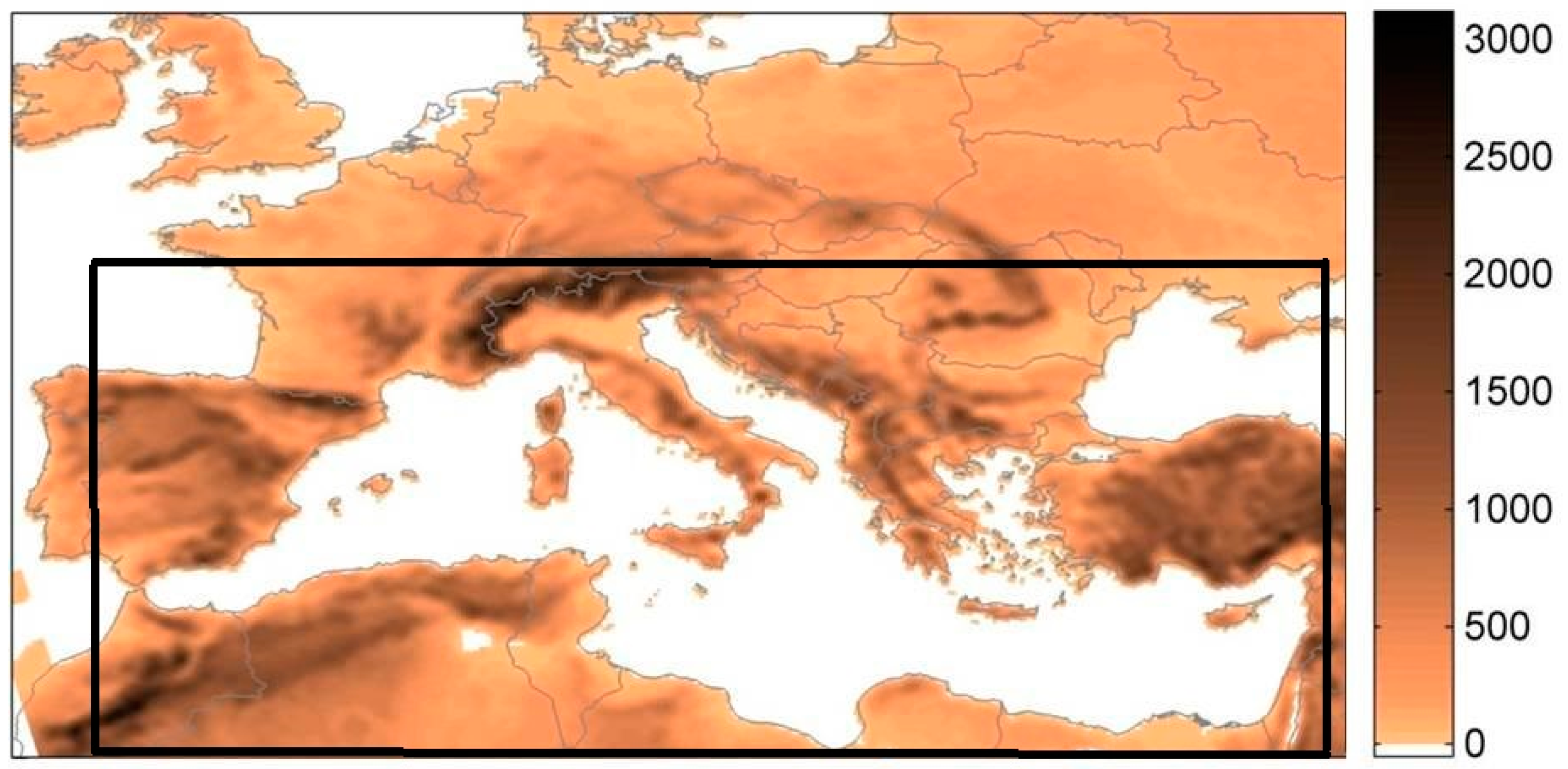
The simulation setup is briefly summarized in Table 1. The model version used to run the simulation is 4.8 CLM13 and the interpolator INT2LM model version 1.10 CLM2. A horizontal resolution of 0.125° (about 14 km) has been adopted. Two simulations have been carried out over the domain −10°–40°E/29°–57°N, shown in Figure 1. The first one driven by the ERA40 Reanalysis [17], characterized by a horizontal resolution of 1.125° (about 128 km) for the time period 1971–2000, in order to assess the capabilities of the model to reproduce the recent past climate of the area considered under “near-perfect boundary conditions”. The second one driven by the global model CMCC-MED [18] for the period 1971–2100 considering the IPCC SRES-A1B emission scenario. CMCC-MED is a coupled atmosphere–ocean general circulation model, whose atmospheric model component is ECHAM5 with a T159 horizontal resolution, corresponding to a Gaussian grid of about 0.75° × 0.75°. This configuration has 31 hybrid sigma-pressure levels in the vertical and top at 10 hPa. The parameterization of convection is based on the Tiedtke scheme; moist processes are treated using a mass-conserving algorithm for the transport of the different water species and potential chemical tracers. The transport is resolved on the Gaussian grid.
2.2. Observational Dataset
The E-OBS dataset [19] has been used for 2-m temperature and precipitation evaluation. It is a European daily high-resolution (0.25° × 0.25°) gridded data set over land points for precipitation, minimum, maximum, and mean surface temperature and for sea level pressure covering the period 1950–2010. It was obtained by using data from 2316 stations, and it has been designed to provide the best estimate of grid box averages rather than point values to enable direct comparison with RCMs.
Gridded datasets, where each grid value is the best average estimate of observations available in the area of the grid box, are the most appropriate ones for the validation of model output, since they are indicative of processes at the same spatial scale. However, gridded datasets derived through interpolation of station data have a number of potential inaccuracies and errors, as they suffer both from measurement errors in the underlying station data and from interpolation errors. In general, interpolation accuracy decreases as the network density decreases, resulting less accurate for variables with more variable spatial characteristics (e.g., precipitation) degrading in complex terrain areas.
Concerning the total cloud cover validation, the ERA-Interim Reanalysis of the global atmosphere [20] has been used instead: They are characterized by a resolution of 0.703° (about 79 km), covering the period since 1979 and continuously updated in real time.
3. Validation
The evaluation of the accuracy of the simulation is performed considering the daily values of a 2-m mean temperature and daily total precipitation, for the period 1971–2000. The validation process involves the analysis of annual cycle, Probability Density Functions (PDF) and time series, obtained considering daily values of the variables of interest, spatially averaged over the Mediterranean area defined as −5°–37° E/29°–47° N, shown in Figure 1. Moreover, model outputs of both ERA40, CMCC-MED driven simulations have been compared in each grid-point of the computational domain, using seasonal means and their differences are displayed in bias maps over the entire domain, in order to quantify the error induced by the global model.
An interesting question, regarding uncertainties of the climate projections with respect to the biases, is whether climate change signals (found by using numerical models) can be influenced by the presence of biases in the model simulations. In our opinion, biases in the base and in the projected years are consistent, implying that projection changes provide a reasonable bias removal. In any case, the use of RCM simulations, as direct input data for impact studies is quite complicated. Therefore, since the impact of climate changes is usually assessed at a local scale, the common state of art approach is to post-process the RCM simulation output to produce reliable estimates of local scale climate. Different bias correction methods may be used to solve the various problems present in the raw RCM model results.
3.1. Temperature
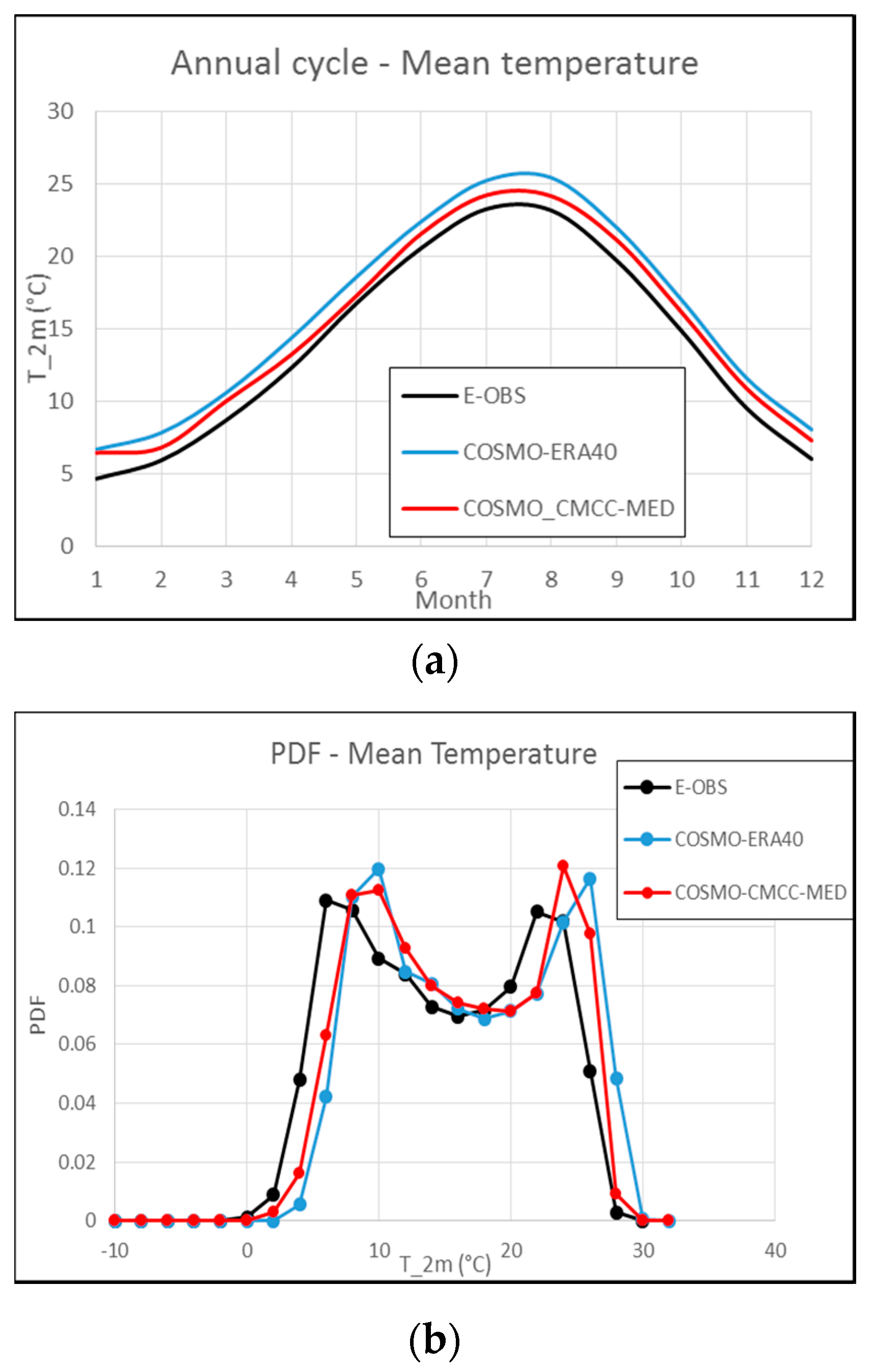
The annual cycle (Figure 2a) shows a good match between model and dataset, with a general overestimation, which is more evident in the ERA40 driven simulation. Concerning the statistical characterization, the daily temperature PDF distributions (Figure 2b) of model and observations show a good agreement, with peaks reached at about 10 °C and 30 °C. Model output registers a higher number of hot extreme values, while E-OBS dataset is characterized by greater density in the middle range. The time series (Figure 3) shows a general increase over the years, by both modeled and observed data, even if with different absolute values. More specifically, E-OBS is characterized by a numerical trend of 0.56 °C per decade, while trends for ERA40 and GCM driven simulations are 0.31 and 0.36 respectively. In this last case, the trend is evaluated over the whole 21st century. It is worth noting that, over the past period, the GCM driven simulation does not indicate a warming trend.
The mean temperature bias maps over the whole area are shown in Figure 4, the ERA40 driven simulation is characterized by an average cold bias of about 2.2 °C in DJF, with highest bias occurring in the Alpine region. In JJA, a strong warm bias up to 4 °C in the eastern part is registered, along with a cold bias of about 2 °C over Alps and northern Spain. These lasts feature could be motivated by the low number of stations available on mountains area for the E-OBS dataset. The shortcoming of COSMO-CLM, leading to underestimation of the winter temperature at high altitudes, has already been highlighted in several works (e.g., [21]). A possible explanation of the summer positive bias is the deficiency of the model in reproducing atmospheric dynamics typical of some areas considered: In fact, many RCM and general circulation models overestimate summer temperature in semiarid regions (e.g., Iberian Peninsula, North Africa) [22].
With the exception of the eastern part in summer, the temperature is quite well reproduced in the ERA40 driven simulation, being the bias lower than the one characterizing most of the typical RCM simulations available on this area. An analysis of PRUDENCE simulations over the whole European area provided in [23] revealed a warm bias for RCMs with respect to the CRU dataset in extreme seasons and a tendency to cold biases in transition seasons. EURO-CORDEX models over the Mediterranean subdomain show non-negligible temperature biases [24]. The CMCC-MED driven simulation is characterized by a cold bias over the whole domain in DJF and in the western part in JJA, while the eastern part in JJA is characterized by a hot bias.
3.2. Precipitation
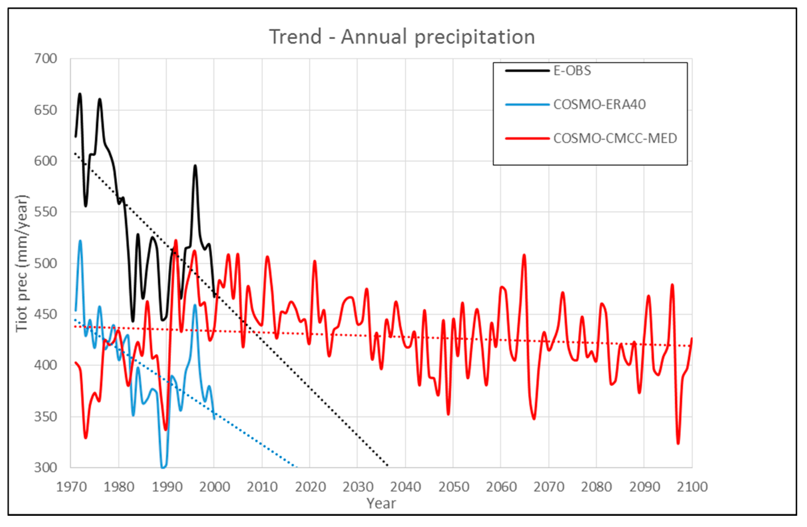
The annual cycle obtained with model data is similar to the observed one, but with an underestimation from March to December (Figure 5a). Looking at mean daily precipitation PDF (Figure 5b), we note that the number of occurrence of low precipitation days (1–2 mm/day) is overestimated by the model. Simulated data have a more rapid decrease and slower decay in distribution compared to E-OBS, but model results proved to have a lower variance than observations. The annual time series (Figure 6) provided by the GCM driven simulation shows a slightly decreasing trend of model data over the future period (−14 mm/year per decade), while over the past period it shows an increasing trend. This is not in agreement with E-OBS time series, which shows a large reduction (−46 mm/year per decade). ERA40-driven model output is generally close to the dataset (−31 mm/year per decade).
Precipitation mostly occurs in DJF, with highest values in mountain areas (up to 8 mm/day) while in JJA, the only worth-to-notice element is a peak on the Alpine region. The precipitation bias maps (Figure 7) reveal no significant differences between the two simulations. The model tends to overestimate in high orography areas (e.g., Alps and Pyrenees), with large differences in DJF (4 mm/day). A large underestimation is observed in Portugal, whereas a better match is registered elsewhere. In JJA, the agreement is better, with a null bias in the southern part where precipitation is close to zero in this season. Over Europe precipitation is slightly underestimated (lesser than 1 mm/day), with the exception of the Alpine area (strong overestimation). The winter overestimation over mountain areas is very likely due to an underestimation of the orographic effects: In presence of a mountainous terrain, the airflow experiences a forced lifting, causing an adiabatic cooling and condensation. This effect can be underestimated, if the resolution of the orography is not fine enough, so an overestimation of the precipitation on the lee side of the mountains may occur [25]. Since summer precipitation is mainly due to convection, the observed bias proves that the model resolution is not fine enough to capture phenomena such as localized convection. An analysis of the ENSEMBLES RCMs shows a tendency to over-predict precipitation, resulting in a total bias of about 20% in winter and less than 10% in summer [26]. The EURO-CORDEX models show generally high precipitation overestimation over Mediterranean, up to 120% in summer [24].
3.3. Total Cloud Cover
Since total cloud cover is not available in the E-OBS dataset, ERA-Interim Reanalysis have been used as a reference for the validation of this variable. Moreover, being the analyzed simulation driven by ERA40 Reanalysis, it is also of interest to compare the total cloud cover of COSMO-CLM output with the ERA40 themselves.
Several authors have already performed a comparison between the results of regional climate models respectively driven by ERA-Interim or ERA40. Cardoso et al. [27], calculated error statistics on the precipitation in the Iberian Peninsula, while Roesch et al. [28] focused on the 2-m mean temperature and Jaeger et al. [29] used the ERA15 and ERA40 data as observational dataset.
According to the ERA-Interim availability, the time period considered is 1979–2000. RCM output has been interpolated onto ERA-Interim grid, whereas for what concerns the comparison between ERA40 and COSMO-CLM, and between ERA40 and ERA-Interim, all the data have been interpolated onto the ERA40 grid (1.125°, about 125 km).
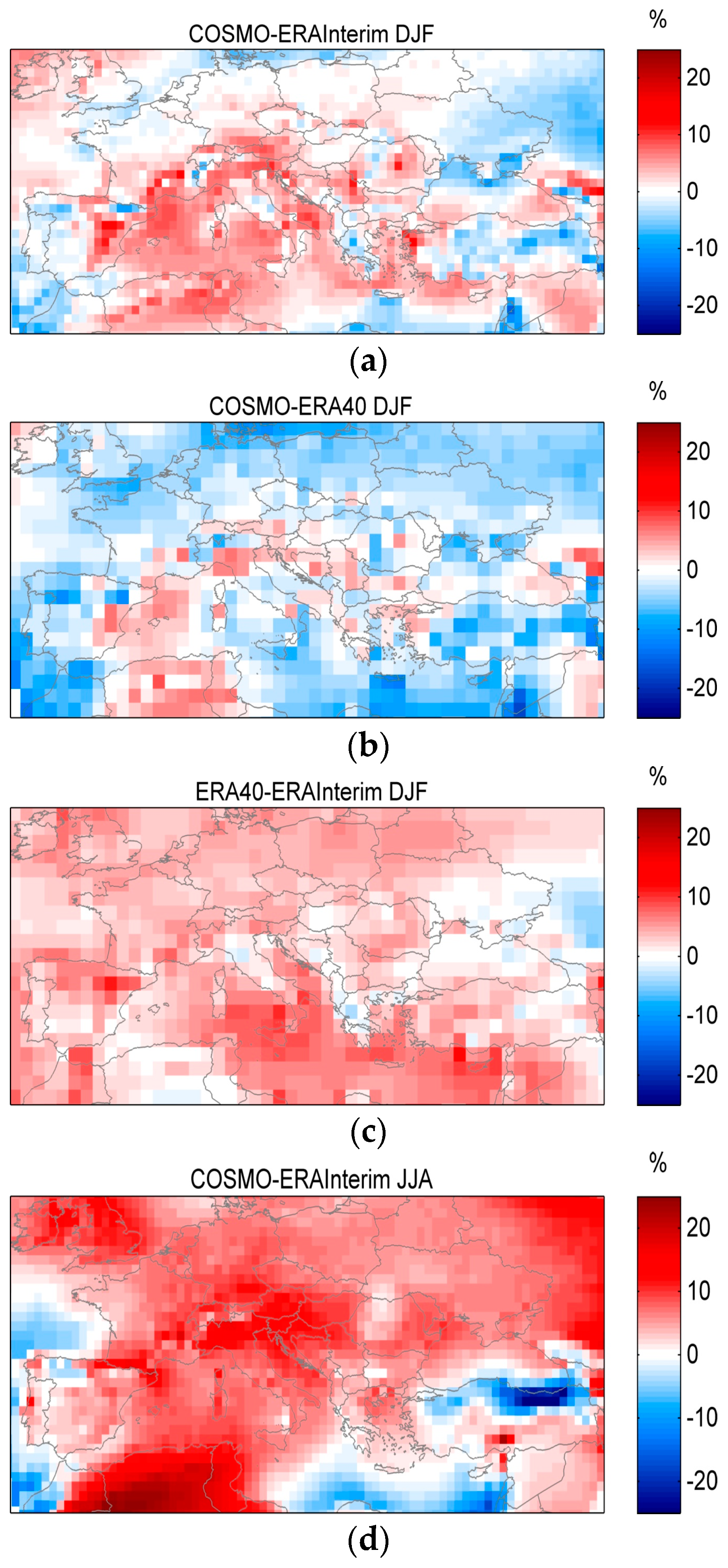
Analyzing the difference between COSMO-CLM and ERA-Interim (Figure 8a,d), a general overestimation of the total cloud cover is observed, especially evident in summer, with a peak of about 20% in the northwest Africa. An opposite trend is found only in the northeast Europe in the winter and in the north coast of Turkey and Israel in the summer. In both winter and autumn, a good agreement is shown, especially in northern Europe. During wintertime, the overestimation in the Mediterranean Sea is especially due to the forcing data. In fact, ERA40 Reanalysis overestimates the total cloud cover with respect to ERA-Interim (Figure 8c,f). This trend is evident also in autumn, when an overestimation in the northern Africa is found due to the regional model.
In spring and summer, COSMO-CLM tends to exacerbate the overestimation already present in the ERA40 data, as shown by the comparison between ERA40 and ERA-Interim (Figure 8, third column), simulating higher cloud cover with respect to its forcing (Figure 8, second column). This explains the higher over-estimation, displayed in the first column of Figure 8. The summer underestimation in Turkey and in Israel can be totally attributed to the regional model, since this pattern is not present in the comparison between ERA40 and ERA-Interim, but it is only present in the comparison between model and its forcing.
In conclusion, COSMO-CLM generally tends to overestimate the total cloud cover especially in summer, but this over-estimation can be partly attributed to the forcing, especially in some seasons and regions.
4. Climate Projections
Climate projections over the 21st Century have been performed using the SRES-A1B emission scenario [11] including long term, global emissions of greenhouse gases, short-lived species, and land-use-land-cover in a global economic framework. It is a stabilization scenario and assumes that climate policies, in this instance the introduction of a set of global greenhouse gas emissions prices, are invoked to achieve the goal of limiting emissions and radiative forcing (CO2 concentration of about 700 ppm by 2100). Compared with the most recent Representative Concentration Pathways (RCPs) [30], A1B places itself between RCP4.5 and RCP8.5 in terms of CO2 mole fraction in the air at the end of 21st century. Moreover, as reported in [31] the global average projected warming under A1B is located between the values of the RCP6 and RCP8.5 scenarios.
In the present work, climate projections were analyzed comparing the average values of 2-m temperature and precipitation for the period 2071–2100 with respect to the period 1971–2000. Figure 9 shows the change of the 2-m temperature distribution, related to DJF (left) and JJA (right). A general increase of temperature is expected in all the examined area, which is consistent with results reported in [2], but provides a greater level of details due to the very high spatial resolution here adopted. In DJF, the strongest increase occurs in the eastern part of the domain, while in Portugal and western France it is moderate. In JJA, an opposite behavior occurs, since Spain and North Africa will experience the largest increase of temperature. It is worth noting that in both DJF and JJA seasons, Italy will be affected by a significant warming (about 4 °C), and this is consistent with the analyses provided in [32].
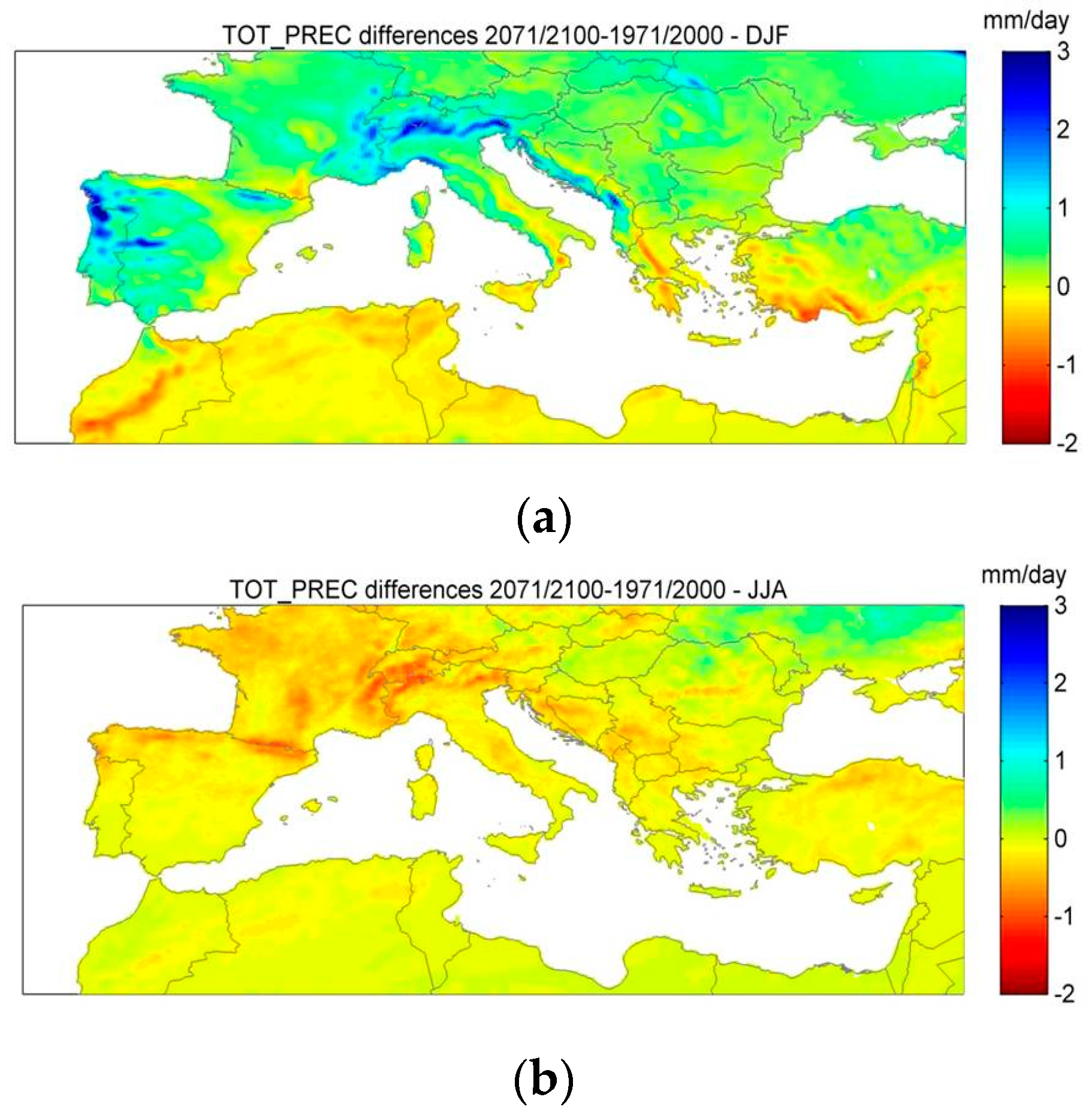
Figure 10 shows the change of total precipitation distribution, related to DJF (left) and JJA (right). In DJF, a precipitation increase in Portugal and on the Alps (up to 270 mm/season, 200%) occurs, while a decrease in North Africa and south Turkey is observed. In JJA a general decrease is observed (up to 185 mm/season, −70%), especially in the northwestern part of the domain. Overall, the general precipitation trends reported in [2] are confirmed by the present results. Concerning Italy, it is affected by a moderate increase in the northwestern part in DJF, while no significant changes are expected in southern Italy in DJF and in the whole domain in JJA. These results confirm only partially the findings reported in [32], so a deeper analysis at higher resolution over Italy was needed and described in [33].
Temperature changes over specific areas are related to precipitation changes and land atmosphere interactions [34,35]. The decreased winter warming over the Alps and the western Iberian Peninsula can be attributed to the projected increase of precipitation over the aforementioned regions. Vice versa, the strong winter drying over the Moroccan highlands can be contributing to the strong temperature increase, which is also the case for Greece and southern Turkey. Similar feedbacks can be found for the summer season over the Alps.
5. Conclusions
An analysis of RCM simulations with COSMO-CLM over the Mediterranean region at the spatial resolution of 0.125° has been presented. The model response has been analyzed in terms of 2-m temperature, precipitation and total cloud cover, making a comparison with the available observations. Results obtained in this process prove that, even if wide areas are affected by non-negligible biases COSMO-CLM is basically able to simulate the main features of the observed climate over the wide area of the Mediterranean Sea. The bias is generally larger on high orography zones, since the model gives colder temperatures and more intense rainfalls in these points. It is worth noting that part of the bias against E-OBS is related to observation inaccuracy, as assessed in [36]. When driven by the GCM, COSMO-CLM shows a deficiency in reproducing the positive temperature trend and the negative precipitation trend over the past period, which are well captured when the model is driven by reanalysis. This shortcoming might be overcome by using different data forcing, also in order to quantify the uncertainty associated with boundary conditions.
The good capabilities of the model in reproducing PDFs observed in the present work, combined with the finding of several literature works (e.g., [33,37]) confirm that, especially in some complex areas, high-resolution simulations could provide good improvements in the data quality. Indeed, there is no ideal resolution appropriate for every geographical area, since it depends on the climate variability of the context considered. Each of the three components of the modeling chain (emission scenario, GCM, RCM) is a potential source of uncertainty that needs to be quantified. GCMs and RCMs are affected by a systematic bias, caused by imperfect conceptualization, discretization and physical parameterization. The model biases make impracticable the use of RCM simulations as direct input data for hydrological impact studies, so a “bias correction” technique is often required.
Climate projections highlight a substantial warming of the Mediterranean region at the end of 21st century, combined with a reduction of precipitation in the warm season, and an increase of precipitation over Alpine space in winter. These results are generally consistent with the findings of other literature works [2], obtained with both global and regional models, also for different emission scenarios, especially for what concerns temperature, while future projected precipitation changes are beset by larger uncertainties. In this context, as assessed in the IPCC report [38], a multi-model ensemble could improve their reliability, especially if single elements are weighted with a measure of the model skill. A possible approach is the Reliability Ensemble Averaging (REA). For this reason, multi-model ensembles must use a common framework to obtain useful conclusions in projecting future climate changes, as addressed for example in the CORDEX project [6] and more specifically in the MED-CORDEX initiative [12].
The present analysis concentrated only on average climate variables, but it is well known that climate extremes have more impacts on society than average values [39]. Hence, in a future work the present simulations will be analyzed in order to provide climate projections of extreme events indicators. For example, the heat waves, unusual in the present climate, are expected to become very common due to the increasing mean temperature, and could occur in any country of the Mediterranean area. Additional trends in extreme temperature may play a significant role in the tendency of heat waves, as documented e.g., in [40]. Since the resilience measures have already reached their limits, especially over northern Africa [41], climate projections of extreme events could be useful to address sustainable solutions for local adaptation.
Author Contributions
The research leading to these results has received funding from the People Programme (Marie Curie Actions) of the European Union’s Seventh Framework Programme (FP7/2007–2013) under REA grant agreement No. 269327 Acronym of the Project: EPSEI (2011–2015) entitled “Evaluating Policies for Sustainable Energy Investments: Towards an Integrated Approach on National and International Stage”, within the results coordinated by gLAWcal—Global Law Initiatives for Sustainable Development and led by Professor Paolo Davide Farah.
Conflicts of Interest
The authors declare no conflict of interest.
References
- Josey, S. Changes in the heat and fresh water forcing of the eastern Mediterranean and their influence on deep water formation. J. Geophys. Res. 2003, 108, 3237. [Google Scholar] [CrossRef]
- Giorgi, F.; Lionello, P. Climate change projections for the Mediterranean region. Glob. Planet. Chang. 2008, 63, 90–104. [Google Scholar] [CrossRef]
- Giorgi, F. Climate change Hot-spots. Geophys. Res. Lett. 2006, 33, L08707. [Google Scholar] [CrossRef]
- Intergovernmental Panel on Climate Change (IPCC). Managing the Risks of Extreme Events and Disasters to Advance Climate Change Adaptation; A Special Report of Working Groups I and II of the Intergovernmental Panel on Climate Change; Field, C.B., Barros, V., Stocker, T.F., Qin, D., Dokken, D.J., Ebi, K.L., Mastrandrea, M.D., Mach, K.J., Plattner, G.-K., Allen, S.K., et al., Eds.; Cambridge University Press: Cambridge, UK; New York, NY, USA, 2012. [Google Scholar]
- Anav, A.; Ruti, P.M.; Artale, V.; Valentini, R. Modelling the effects of land-cover changes on surface climate in the Mediter ranean region. Clim. Res. 2010, 41, 104. [Google Scholar] [CrossRef]
- Giorgi, F.; Jones, C.; Asrar, G.R. Addressing climate information needs at the regional level: The CORDEX framework. WMO Bull. 2009, 58, 175–183. [Google Scholar]
- Senatore, A.; Mendicino, G.; Smiatek, G.; Kunstmann, H. Regional climate change projections and hydrological impact analysis for a Mediterranean basin in Southern Italy. J. Hydrol. 2011, 399, 70–92. [Google Scholar] [CrossRef]
- Christensen, J.H.; Christensen, O.B. A summary of the PRUDENCE model projections of change in European climate by the end of this century. Clim. Chang. 2007, 81, 7–30. [Google Scholar] [CrossRef]
- Van Der Linden, P.; Mitchell, J. Ensembles: Climate Change and Its Impacts: Summary of Research and Results from the Ensembles Project; Met Office Hadley Centre: Exeter, UK, 2009; p. 160. [Google Scholar]
- Rockel, B.; Will, A.; Hense, A. The regional climate model cosmo-clm (cclm). Meteorol. Z. 2008, 17, 347–348. [Google Scholar] [CrossRef]
- Intergovernmental Panel on Climate Change (IPCC). Towards New Scenarios for Analysis of Emissions, Climate Change, Impacts, and Response Strategies; IPCC Expert Meeting Report; Intergovernmental Panel on Climate Change: Geneva, Switzerland, 2008. [Google Scholar]
- Ruti, P.; Somot, S.; Giorgi, F.; Dubois, C.; Flaounas, E.; Obermann, A.; Dell’Aquila, A.; Pisacane, G.; Harzallah, A.; Lombardi, E.; et al. Med-CORDEX Initiative for Mediterranean Climate Studies. Bull. Am. Meteorol. Soc. 2016, 97, 1187–1208. [Google Scholar] [CrossRef] [Green Version]
- Rockel, B.; Geyer, B. The performance of the regional climate model clm in different climate regions, based on example of precipitation. Meteorol. Z. 2008, 17, 487–498. [Google Scholar] [CrossRef]
- Steppeler, J.; Doms, G.; Schattler, U.; Bitzer, H.W.; Gassmann, A.; Damrath, U.; Gregoric, G. Meso-gamma scale forecasts using the nonhydrostatic model lm. Meteorol. Atmos. Phys. 2003, 82, 75–96. [Google Scholar] [CrossRef]
- Bohm, U.; Kucken, M.; Ahrens, A.; Block, A.; Hauffe, D.; Keuler, K.; Rockel, B.; Will, A. CLM the climate version of LM: Brief description and long term applications. COSMO Newslett. 2006, 6, 225–235. [Google Scholar]
- Schär, C.; Leuenberger, D.; Fuhrer, O.; Lüthi, D.; Girard, C. A New Terrain-Following Vertical Coordinate Formulation for Atmospheric Prediction Models. Mon. Weather. Rev. 2002, 130, 2459–2480. [Google Scholar] [CrossRef]
- Uppala, S.M.; Kallberg, P.W.; Simmons, A.J.; Andrae, U.; Da Costa Bechtold, V.; Fiorino, M.; Gibson, J.K.; Haseler, J.; Hernandez, A.; Kelly, G.A.; et al. The era-40 re-analysis. Q. J. R. Meteorol. Soc. 2006, 612, 2961–3012. [Google Scholar] [CrossRef]
- Gualdi, S.; Somot, S.; Li, L.; Artale, V.; Adani, M.; Bellucci, A.; Braun, A.; Calmanti, S.; Carillo, A.; Dell’Aquila, A.; et al. The CIRCE Simulations: Regional Climate Change Projections with Realistic Representation of the Mediterranean Sea. Bull. Am. Meteorol. Soc. 2013, 94, 65–81. [Google Scholar] [CrossRef] [Green Version]
- Haylock, M.R.; Hofstra, N.; Klein Tank, A.M.G.; Klok, E.J.; Jones, P.D.; New, M. A European daily high-resolution gridded data set of surface temperature and precipitation for 1950–2006. J. Geophys. Res. 2008, 113. [Google Scholar] [CrossRef]
- Dee, D.S.; Uppala, M.; Simmons, A.J.; Berrisford, P.; Poli, P.; Kobayashi, S.; Andrae, U.; Balmaseda, M.A.; Balsamo, G.; Bauer, P.; et al. The era-interim reanalysis: Configuration and performance of the data assimilation system. Q. J. R. Meteorol. Soc. 2011, 137, 553–597. [Google Scholar] [CrossRef]
- Haslinger, K.; Anders, I.; Hofstätter, M. Regional climate modelling over complex terrain: an evaluation study of COSMO-CLM hindcast model runs for the Greater Alpine Region. Clim. Dyn. 2012, 40, 511–529. [Google Scholar] [CrossRef]
- Boberg, F.; Christensen, J.H. Overestimation of Mediterranean summer temperature projections due to model deficiencies. Nat. Clim. Chang. 2012, 2, 433–436. [Google Scholar] [CrossRef]
- Jacob, D.; Bärring, L.; Christensen, O.B.; Christensen, J.H.; de Castro, M.; Déqué, M.; Giorgi, F.; Hagemann, S.; Hirschi, M.; Jones, R.; et al. Aninter-comparison of regional climate models for Europe: Model performance in Present-Day Climate. Clim. Chang. 2007, 81, 31–52. [Google Scholar] [CrossRef]
- Kotlarski, S.; Kriegsmann, A.; Martin, E.; van Meijgaard, E.; Moseley, C.; Pfeifer, S.; Preuschmann, S.; Radermacher, C.; Radtke, K.; Rechid, D.; et al. EURO-CORDEX: New high-resolution climate change projections for European impact research. Reg. Environ. Chang. 2014, 14, 563–578. [Google Scholar]
- Bucchignani, E.; Sanna, A.; Gualdi, S.; Castellari, S.; Schiano, P. Simulation of the climate of the XX century in the Alpine space. Nat. Hazards 2011, 67, 981–990. [Google Scholar] [CrossRef]
- Rauscher, S.A.; Coppola, E.; Piani, C.; Giorgi, F. Resolution effects on regional climate model simulations of seasonal precipitation over Europe. Clim. Dyn. 2009, 35, 685–711. [Google Scholar] [CrossRef]
- Cardoso, R.M.; Soares, P.M.; Miranda, P.M.; Belo-Pereira, M. A WRF high resolution simulation of Iberian mean and extreme precipitation climate. Int. J. Climatol. 2013, 33, 2591–2608. [Google Scholar] [CrossRef]
- Roesch, A.; Jaeger, E.B.; Luthi, D.; Seneviratne, S.I. Analysis of CCLM model biases in relation to intra-ensemble model variability. Meteorol. Z. 2008, 17, 369–382. [Google Scholar] [CrossRef]
- Jaeger, E.B.; Anders, I.; Luthi, D.; Rockel, B.; Schar, C.; Senevratne, S.I. Analysis of ERA40-driven CLM simulations for Europe. Meteorol. Z. 2008, 17, 349–367. [Google Scholar] [CrossRef]
- Moss, R.; Edmonds, J.; Hibbard, K.; Manning, M.; Rose, S.; van Vuuren, D.P.; Carter, T.; Emori, S.; Kainuma, M.; Kram, T.; et al. The next generation of scenarios for climate change research and assessment. Nature 2010, 463, 747–756. [Google Scholar] [CrossRef] [PubMed]
- Zittis, G.; Hadjinicolaou, P.; Fnais, M.; Lelieveld, J. Projected changes in heat wave characteristics in the eastern Mediterranean and the Middle East. Reg. Environ. Chang. 2016, 16, 1863–1876. [Google Scholar] [CrossRef]
- Coppola, E.; Giorgi, F. An assessment of temperature and precipitation change projections over Italy from recent global and regional climate model simulations. Int. J. Climatol. 2010, 30, 11–32. [Google Scholar] [CrossRef]
- Bucchignani, E.; Montesarchio, M.; Zollo, A.L.; Mercogliano, P. High-resolution climate simulations with COSMO-CLM over Italy: performance evaluation and climate projections for the 21st century. Int. J. Clim. 2015, 36, 735–756. [Google Scholar] [CrossRef]
- Seneviratne, S.; Corti, T.; Davin, E.; Hirschi, M.; Jaeger, E.; Lehner, I.; Orlowsky, B.; Teuling, A. Investigating soil moisture–climate interactions in a changing climate: A review. Earth Sci. Rev. 2010, 99, 125–161. [Google Scholar] [CrossRef]
- Zittis, G.; Hadjinicolaou, P.; Lelieveld, J. Role of soil moisture in the amplification of climate warming in the eastern Mediterranean and the Middle East. Clim. Res. 2014, 59, 27–37. [Google Scholar] [CrossRef]
- Turco, M.; Zollo, A.; Ronchi, C.; De Luigi, C.; Mercogliano, P. Assessing gridded observations for daily precipitation extremes in the Alps with a focus on northwest Italy. Nat. Hazards Earth Syst. Sci. 2013, 13, 1457–1468. [Google Scholar] [CrossRef]
- Zollo, A.L.; Rillo, V.; Bucchignani, E.; Montesarchio, M.; Mercogliano, P. Extreme temperature and precipitation events over Italy: assessment of high-resolution simulations with COSMO-CLM and future scenarios. Int. J. Clim. 2015, 36, 987–1005. [Google Scholar] [CrossRef]
- Knutti, R.; Abramowitz, G.; Collins, M.; Eyring, V.; Gleckler, P.J.; Hewitson, B.; Mearns, L. Good practice guidance paper on assessing and combining multi model climate projections. In Meeting Report of the Intergovernmental Panel on Climate Change Expert Meeting on Assessing and Combining Multi Model Climate Projections; Stocker, T.F., Qin, D., Plattner, G.K., Tignor, M., Midgley, P.M., Eds.; IPCC Working Group I Technical Support Unit, University of Bern: Bern, Switzerland, 2010. [Google Scholar]
- Klein Tank, A.M.G.; Zwiers, F.; Zhang, X. Guidelines on Analysis of Extremes in a Changing Climate in Support of Informed Decisions for Adaptation; WCDMP-No. 72, WMO-TD No. 1500; World Meteorological Organization, Climate Data and Monitoring: Geneva, Switzerland, 2009. [Google Scholar]
- Wouters, H.; de Ridder, K.; Poelmans, L.; Willems, P.; Brouwers, J.; Hosseinzadehtalaei, P.; Tabari, H.; Broucke, S.V.; van Lipzig, N.P.M.; Demuzere, M. Heat stress increase under climate change twice as large in cities as in rural areas: A study for a densely populated midlatitude maritime region. Geophys. Res. Lett. 2017, 44, 8997–9007. [Google Scholar] [CrossRef]
- Intergovernmental Panel on Climate Change (IPCC). Climate Change 2014: Impacts, Adaptation, and Vulnerability: B. Regional Aspects; Contribution of Working Group II to the Fifth Assessment Report of the Intergovernmental Panel on Climate Change; Barros, V.R., Ed.; Cambridge University Press: Cambridge, UK, 2014. [Google Scholar]
Figure 1.
Orography of the domain. The black line defines the “Mediterranean area” used for the analysis.
Figure 1.
Orography of the domain. The black line defines the “Mediterranean area” used for the analysis.

Figure 2.
Annual cycle (a) and PDF (b) of 2-m temperature, period 1971–2000, averaged over the Mediterranean area.
Figure 2.
Annual cycle (a) and PDF (b) of 2-m temperature, period 1971–2000, averaged over the Mediterranean area.

Figure 3.
Time series of 2-m temperature and trend lines, period 1971–2100, averaged over the Mediterranean area.
Figure 3.
Time series of 2-m temperature and trend lines, period 1971–2100, averaged over the Mediterranean area.
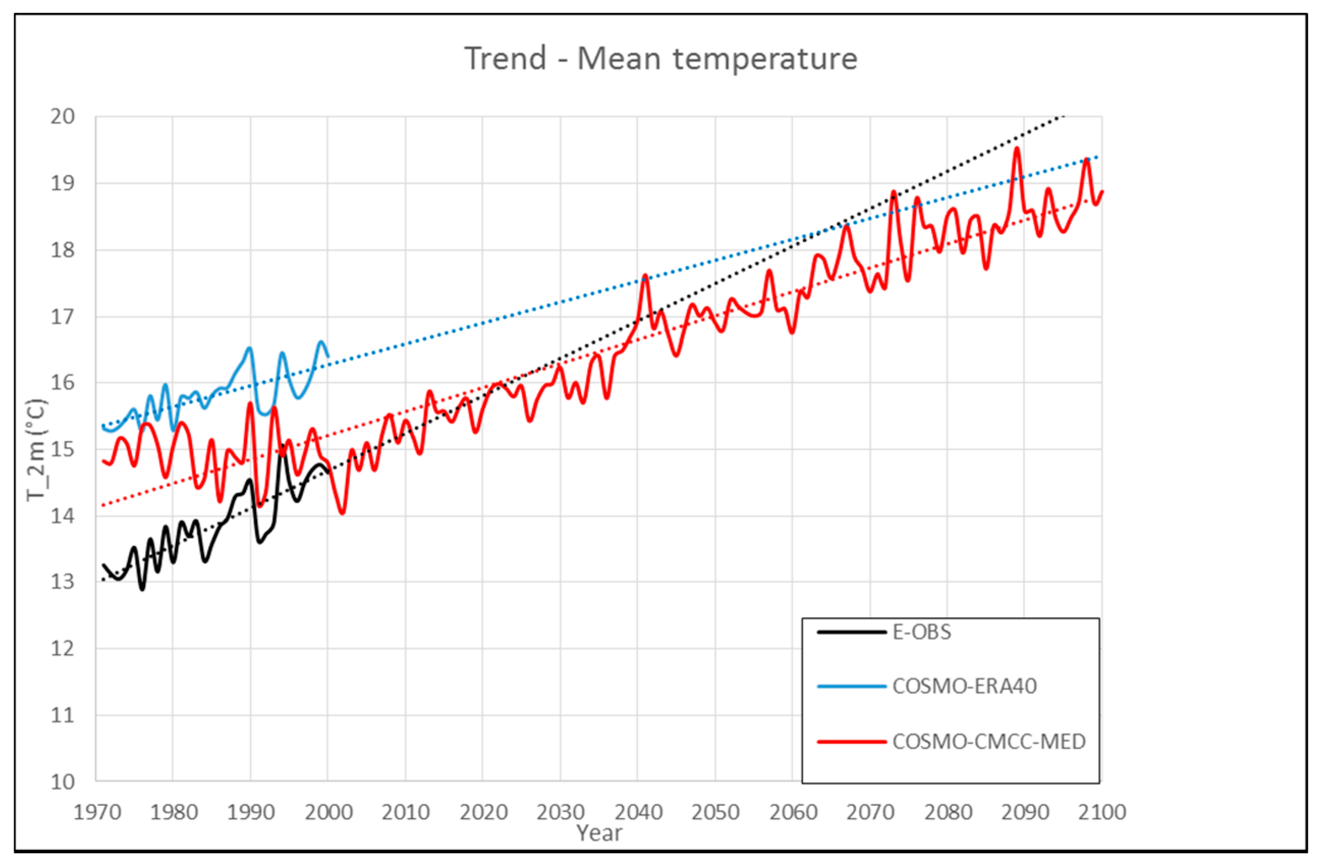
Figure 4.
Seasonal mean bias of 2-meter temperature (over land) with respect to E-OBS dataset, period 1971–2000. ERA-40 driven simulation (a,c): DJF (a,b), JJA (c,d). CMCC-MED driven simulation (b,d): DJF (a,b), JJA (c,d).
Figure 4.
Seasonal mean bias of 2-meter temperature (over land) with respect to E-OBS dataset, period 1971–2000. ERA-40 driven simulation (a,c): DJF (a,b), JJA (c,d). CMCC-MED driven simulation (b,d): DJF (a,b), JJA (c,d).
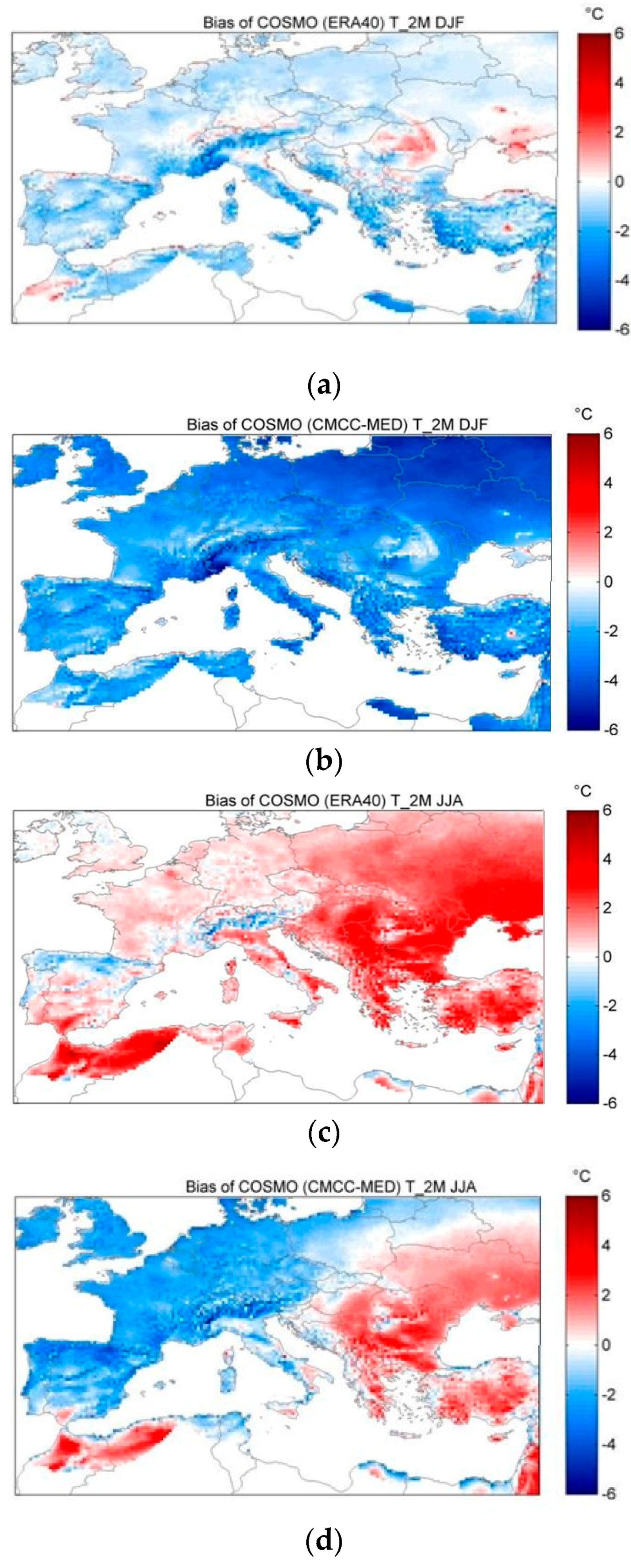
Figure 5.
Annual cycle (a) and PDF (b) of total precipitation, period 1971–2000, averaged over the Mediterranean area.
Figure 5.
Annual cycle (a) and PDF (b) of total precipitation, period 1971–2000, averaged over the Mediterranean area.
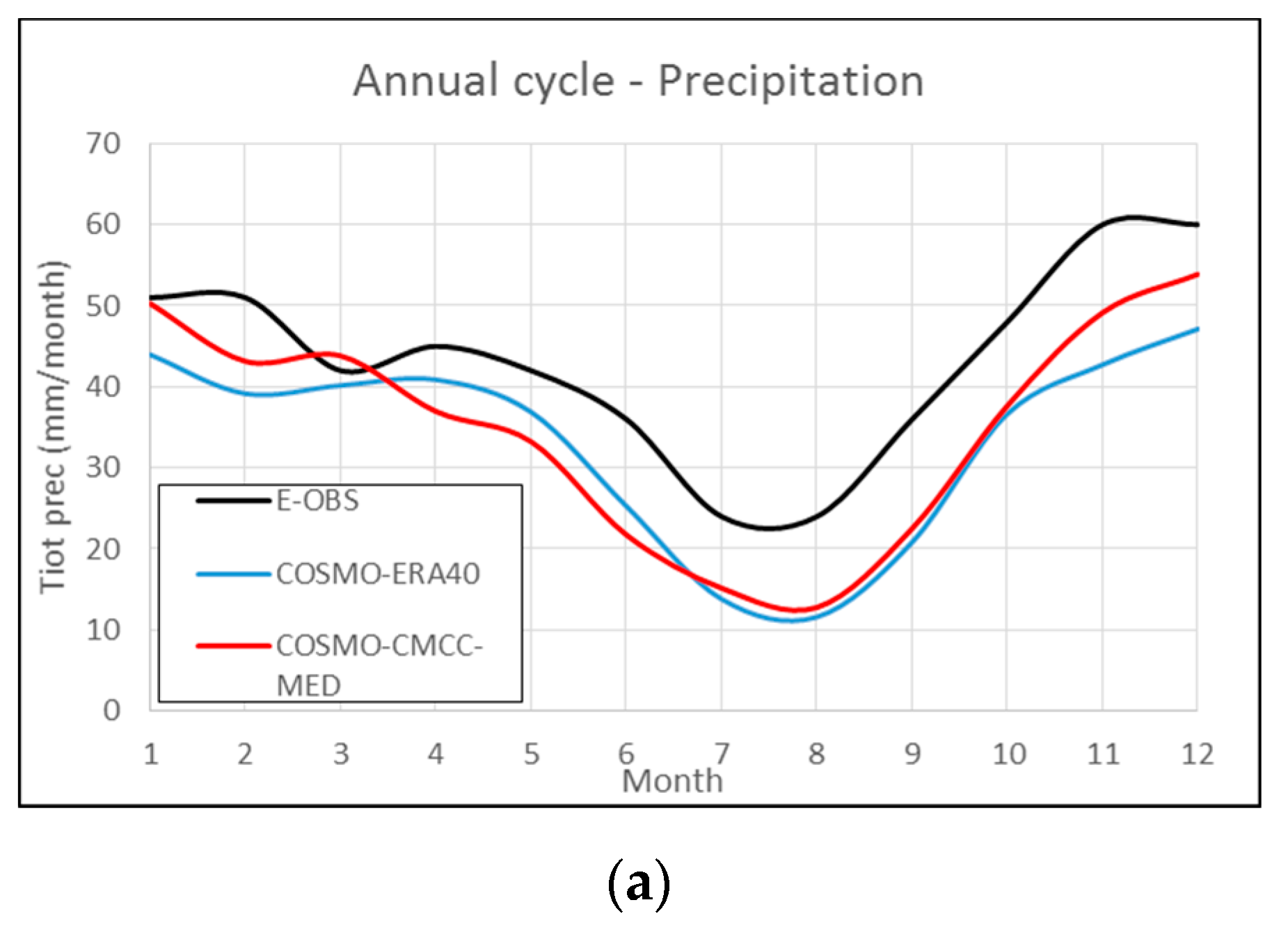
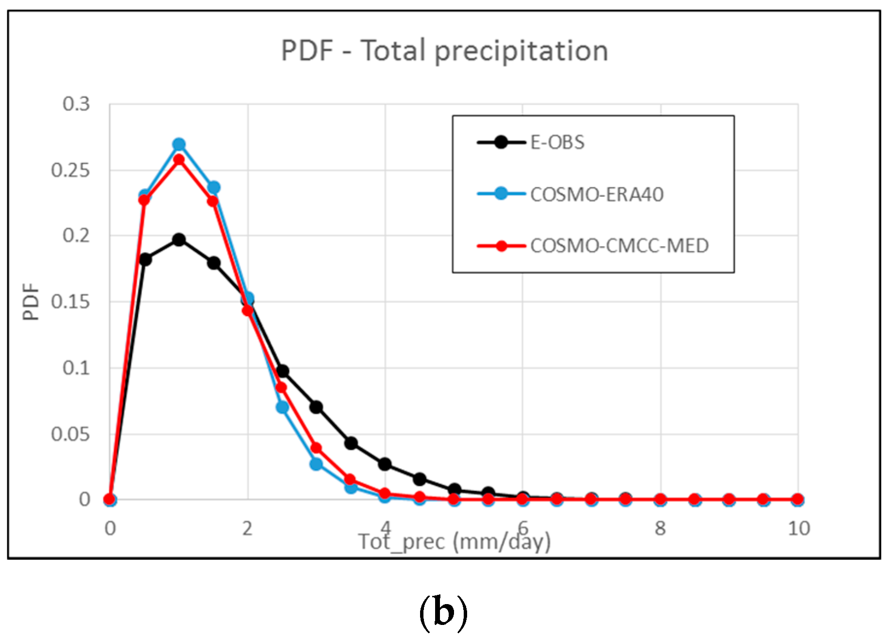
Figure 6.
Time series of total precipitation and trend lines, period 1971–2100, averaged over the Mediterranean area.
Figure 6.
Time series of total precipitation and trend lines, period 1971–2100, averaged over the Mediterranean area.

Figure 7.
Seasonal mean bias of total precipitation (over land) with respect to E-OBS dataset, time period 1971–2000. ERA-40 driven simulation (a,c): DJF (a,b), JJA (c,d). CMCC-MED driven simulation (b,d): DJF (a,c), JJA (b,d).
Figure 7.
Seasonal mean bias of total precipitation (over land) with respect to E-OBS dataset, time period 1971–2000. ERA-40 driven simulation (a,c): DJF (a,b), JJA (c,d). CMCC-MED driven simulation (b,d): DJF (a,c), JJA (b,d).
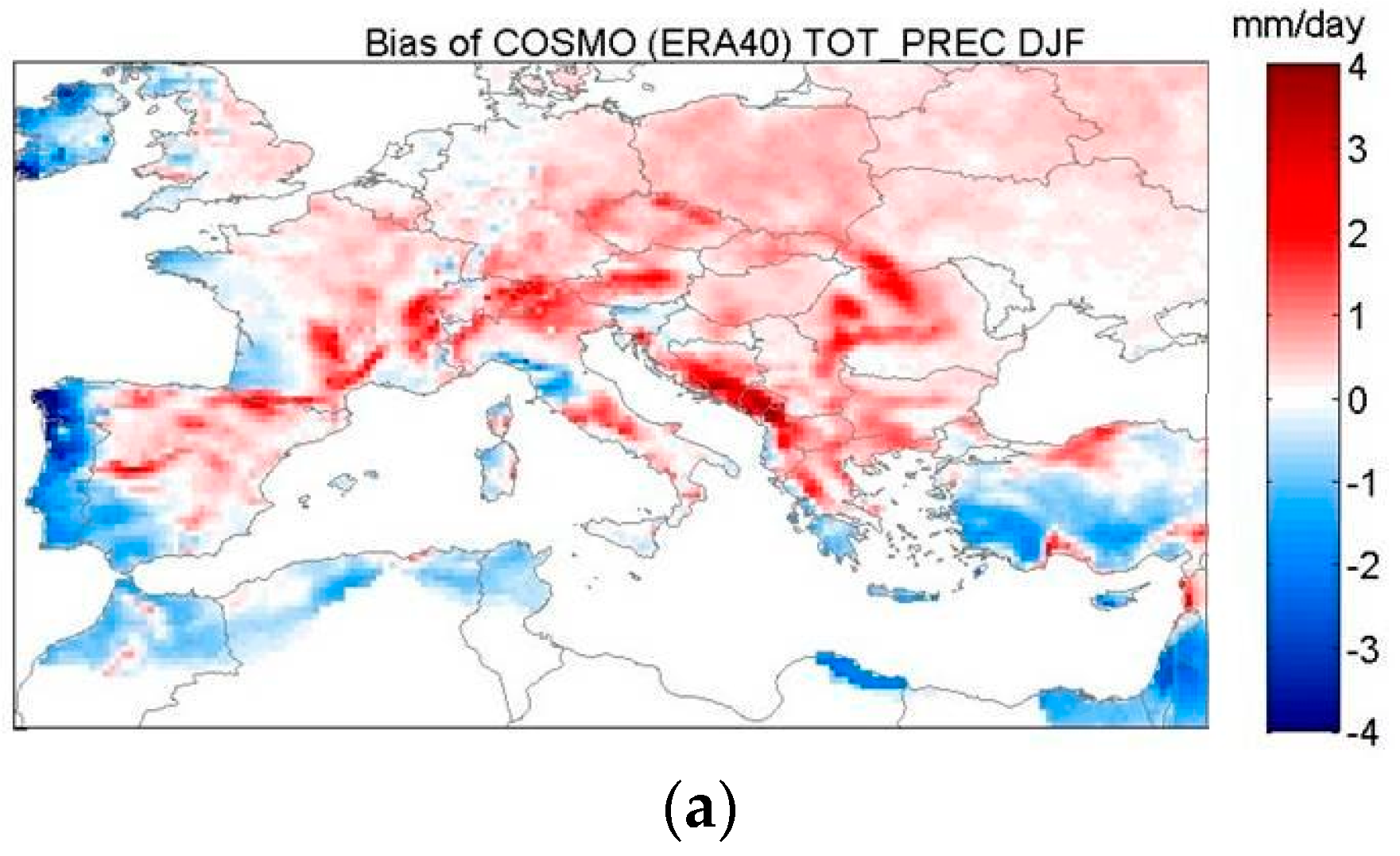
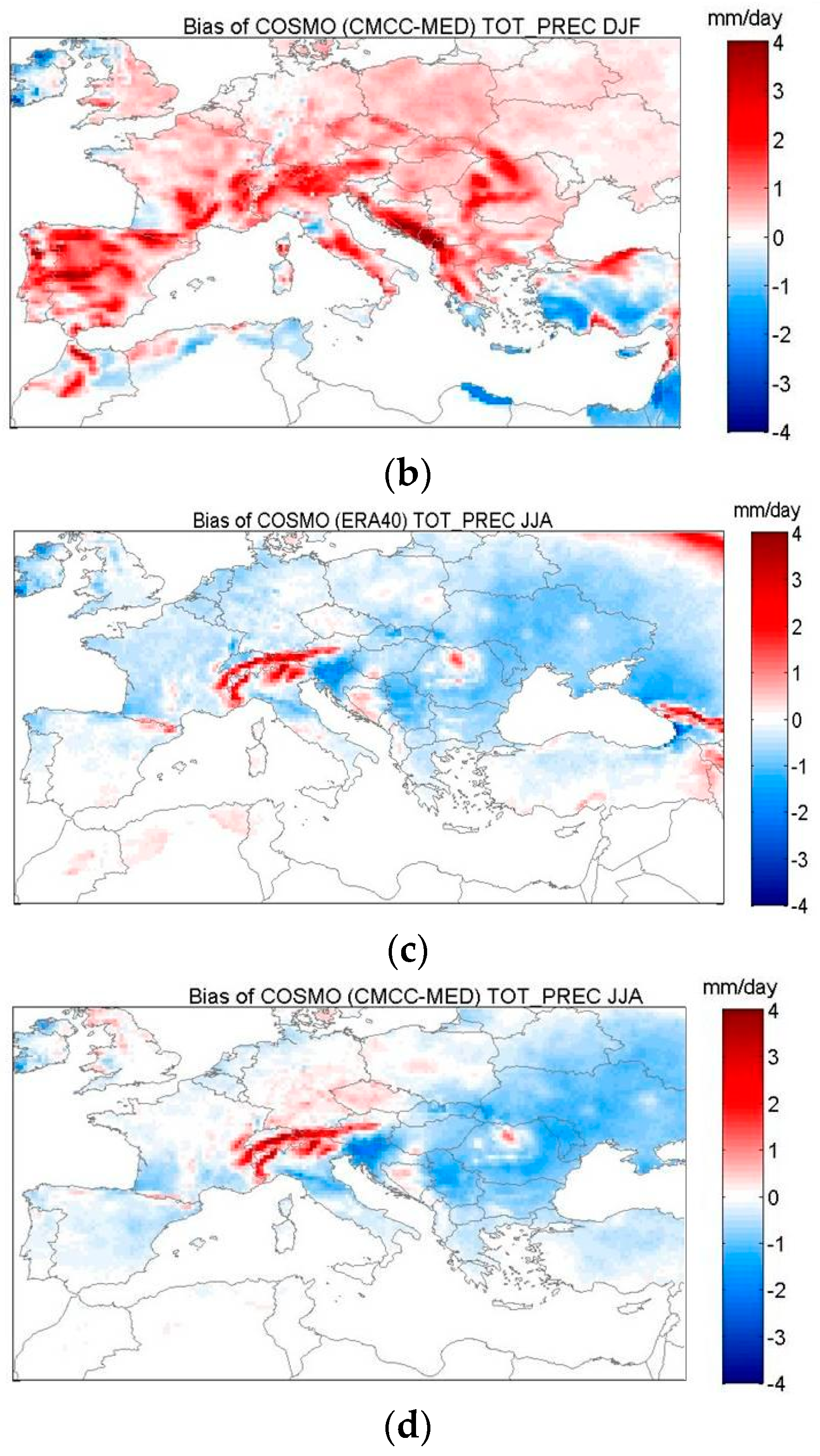
Figure 8.
Seasonal mean bias of total cloud cover, period 1979–2000: COSMO-CLM vs. Era-Interim (a,d), COSMO-CLM vs. ERA-40 (b,e), ERA40 vs. ERA-Interim (c,f).
Figure 8.
Seasonal mean bias of total cloud cover, period 1979–2000: COSMO-CLM vs. Era-Interim (a,d), COSMO-CLM vs. ERA-40 (b,e), ERA40 vs. ERA-Interim (c,f).

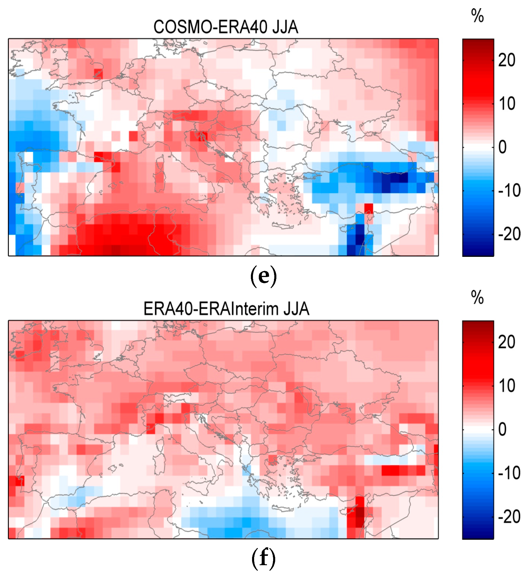
Figure 9.
Climate projections of 2-m temperature over land: Difference between the average values over 2071–2100 and 1971–2000, DJF (a) and JJA (b).
Figure 9.
Climate projections of 2-m temperature over land: Difference between the average values over 2071–2100 and 1971–2000, DJF (a) and JJA (b).
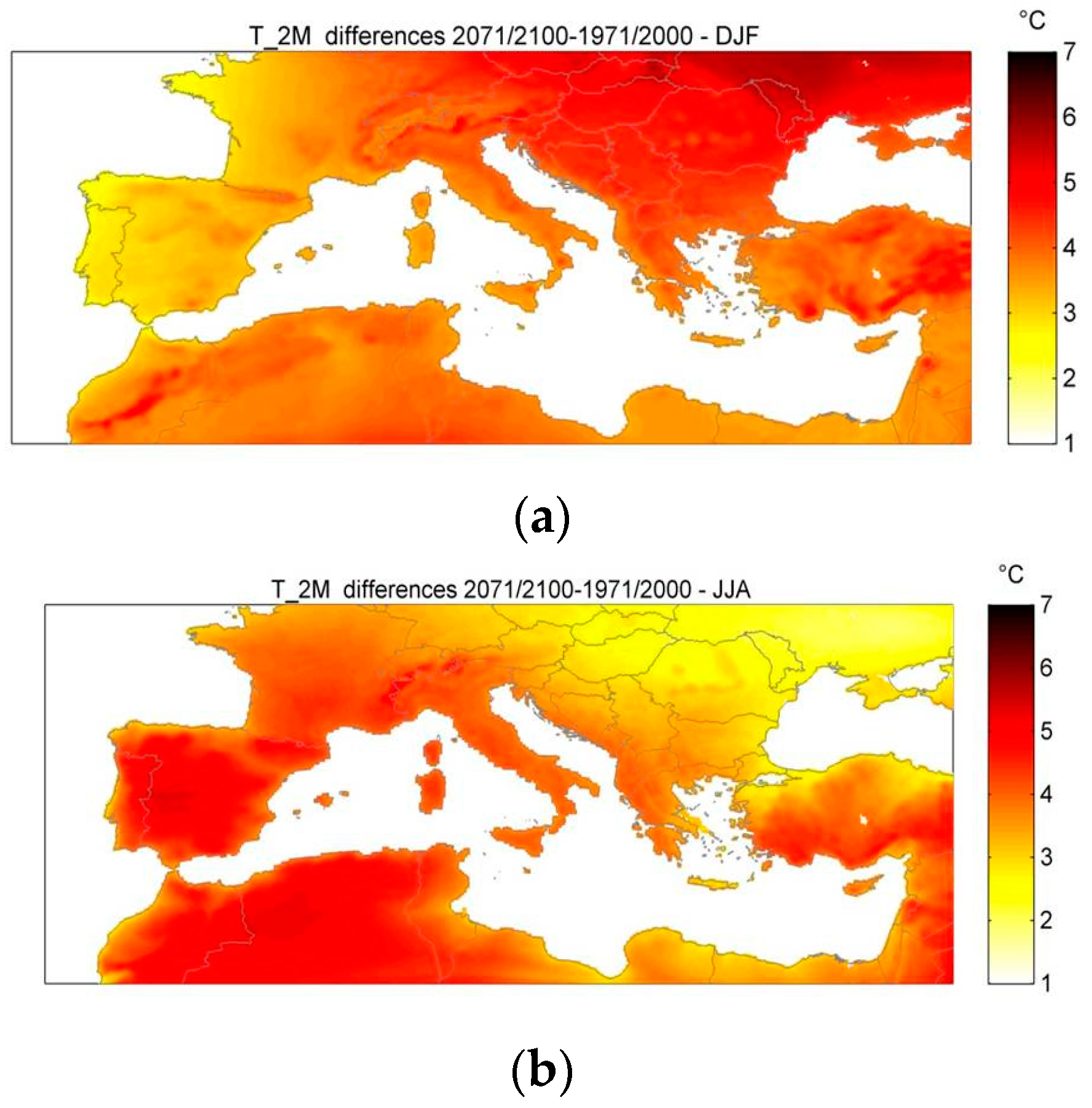
Figure 10.
Climate projections of total precipitation over land: Difference between the average values over 2071–2100 and 1971–2000, DJF (a) and JJA (b).
Figure 10.
Climate projections of total precipitation over land: Difference between the average values over 2071–2100 and 1971–2000, DJF (a) and JJA (b).

Table 1.
Main features of COSMO-CLM setup.
| Driving Data | ERA40 and CMCC-MED |
|---|---|
| Horizontal resolution | 0.125° (about 14 km) |
| Num. of grid points | 385 × 265 |
| Num. of vertical levels | 40 |
| Soil Scheme | TERRA-ML |
| Time step | 150 s |
| Melting processes | Yes |
| Convection Scheme | Tiedke |
| Freq. Radiation comput. | 1 h |
| Time integration | Runge-Kutta 3rd order |
| Freq. update B.C. | 6 h |
© 2017 by the authors. Licensee MDPI, Basel, Switzerland. This article is an open access article distributed under the terms and conditions of the Creative Commons Attribution (CC BY) license (http://creativecommons.org/licenses/by/4.0/).
Share and Cite
MDPI and ACS Style
Edoardo, B.; Paola, M.; Myriam, M.; Lucia, Z.A. Numerical Simulation of the Period 1971–2100 over the Mediterranean Area with a Regional Model, Scenario SRES-A1B. Sustainability 2017, 9, 2192. https://doi.org/10.3390/su9122192
AMA Style
Edoardo B, Paola M, Myriam M, Lucia ZA. Numerical Simulation of the Period 1971–2100 over the Mediterranean Area with a Regional Model, Scenario SRES-A1B. Sustainability. 2017; 9(12):2192. https://doi.org/10.3390/su9122192
Chicago/Turabian StyleEdoardo, Bucchignani, Mercogliano Paola, Montesarchio Myriam, and Zollo Alessandra Lucia. 2017. "Numerical Simulation of the Period 1971–2100 over the Mediterranean Area with a Regional Model, Scenario SRES-A1B" Sustainability 9, no. 12: 2192. https://doi.org/10.3390/su9122192
Note that from the first issue of 2016, this journal uses article numbers instead of page numbers. See further details here.