Article

An Integrated Approach to Evaluating and Selecting Green Logistics Providers for Sustainable Development

1
Department of Industrial Engineering and Management, Fortune Institute of Technology, Kaohsiung 83160, Taiwan
2
Department of Industrial Engineering and Management, National Kaohsiung University of Applied Sciences, Kaohsiung 80778, Taiwan
3
Department of Business Administration, Fortune Institute of Technology, Kaohsiung 83160, Taiwan
4
Department of Management Information Systems, National Chengchi University, Taipei 11605, Taiwan
*
Authors to whom correspondence should be addressed.
Sustainability 2017, 9(2), 218; https://doi.org/10.3390/su9020218
Submission received: 23 November 2016 / Revised: 22 January 2017 / Accepted: 27 January 2017 / Published: 6 February 2017
(This article belongs to the Special Issue Sustainability in Manufacturing)

Abstract

:
Balancing economic development with environmental protection has become a critical concern worldwide. However, along with the highly competitively global marketplace, economic factors are known to directly affect an enterprise’s development and its future business. Therefore, selecting the right partner for sustainable collaboration that will lead to improved business performance and reduce carbon dioxide (CO2) emissions is a significant problem for many enterprises. In addition, investigating the economic impact of companies that are charged to protect the environment is becoming increasingly problematic. Thus, the purpose of this paper is to evaluate the comparative efficiencies of 16 Green Logistics Providers (GLPs) in the USA from 2012 to 2015, and the projected four-year period of 2016–2019, by means of an integrated approach that combines the grey forecasting model GM (1,1) and Data Envelopment Analysis (DEA). The results show that there are two GLPs, Knight Transportation and the Union Pacific Corporation, that possess a higher efficiency level and are achieving positive technical change. However, this study also determined that Hyster-Yale Materials Handling and CSX Corporation did not reach an acceptable efficiency score; therefore, they should improve technical efficiency to mitigate environmental concerns. This completely integrative methodology has the potential to provide the best decision-making strategies for finding suitable collaborative partners who are able to meet the sustainability requirements in most economic and environmental areas.

1. Introduction

Logistics providers play an increasingly important role in maintaining business competitiveness and sustainability, as well as demonstrating social responsibility [1]. However, the U.S. Environmental Protection Agency [2] estimated that nearly 26% of all greenhouse emissions in 2014 resulted from transportation and logistical activities. On the other hand, the logistics industry as a whole has demonstrated its concern to be of equal strategic involvement in achieving lowered CO2 emissions while sustaining positive economic development. The way forward begins by recognizing that the logistics industry itself is a major source of CO2 emissions, accounting for a 13.1% portion of global greenhouse gas emissions. In 2011, China, the United States, India, the Russian Federation, Japan, Canada, and the European Union were the top carbon dioxide (CO2) emitters. Emissions are formed from fossil fuel combustion, cement manufacturing, and petro-gas flaring. In an effort to tackle global warming issues, the logistics industry has proposed implementing and then enforcing consistent environmental measures, especially in the U.S. logistics industry [3].
Facing the economic downturn, the efficient use of natural resources has become essential for sustainable growth [4]. Logistics providers with integrated economic and ecological objectives can help reduce the undesirable impact on the environment by reducing the amount of carbon dioxide emissions created and improving operations efficiency [1]. Seroka [5] pointed out that, in the past, firms coordinated their logistics activities including freight transport, warehousing, packaging, materials handling, data collection, and management to reach customer requirements at minimum cost. However, nowadays, because of the evident environmental impact, some companies have incurred external costs of logistics related with the environmental problems, such as climate change, pollution, and noise abatement. As a result, logistics providers are frequently demanded to improve their green qualifications and sustainability capabilities in order to support the environment [4].
The importance of doing business with logistics firms that demonstrate a real commitment to sustainability in economic and green best practices in their supply chain cannot be underestimated. Concept awareness of sustainability has become increasingly important for organizations, and has permeated a number of managerial and organizational decisions, especially in the logistics industry [6,7]. The sustainable improvement of logistics calls for actions that lead to the highest economic and social benefits while reducing environmental losses. However, in the long term, these activities deal with challenges of sustainable development [8]. As a result, Van Marrewijk and Were [9] stated that each organization should choose its own specific ambition and approach regarding corporate sustainability in order to match the organization’s aims. Therefore, it is significant to consider economic factors in green logistics providers’ (GLPs) operations and evaluate the economic sustainability of GLPs in light of such considerations.
As this study has previously mentioned, it is necessary to understand a company’s past, current, and future process performance to assess improvement options. Thus, the purpose of this research is to evaluate and forecast the operational performance of 16 green logistics companies in the U.S. logistics industry in order to assist potential investors/shareholders in choosing a suitable logistics partner to improve their own business performance and reduce direct impact on climate change. We have used a super slacks-based model (super SBM) model for ranking companies, and have followed it with a Malmquist index to measure the efficiency change, technical change, and productivity change during the past four years, 2012–2015, and for the next four-year period (2016–2019) of forecasting. Finally, with a combined DEA and grey method, this paper has identified the optimal green logistics partnerships and their competitiveness levels within the period 2012–2019. Furthermore, the study also provides useful information for decision makers on selecting suitable partners under the condition of economic benefits for sustainable development.
The organization of this paper is as follows. The next section presents the literature review as it relates to green logistics, economic sustainability, the proposed grey GM (1,1) model, and DEA. Section 3 explains the research methodologies employed. Section 4 provides the empirical results, discussions, and conclusions resulting from this study.

2. Literature Review

2.1. Green Logistics Providers

Logistics focuses on the transfer of goods, sharing information, and the coordination of this overall process. Moreover, the logistics process mostly focuses on optimization, reducing costs, increasing delivery speed, and gaining maximal revenue [10]. However, “green” logistics providers (i.e., environmentally responsible and sustainable) have also been identified as an important factor in the environmental and supply chain strategies of a large number of companies of late. Many studies exploring different aspects of green logistics providers can be found in the literature [5]. Green logistics providers are involved with producing and distributing goods in a sustainable way, taking into account the surrounding environmental and social factors [11]. Similarly, Chunguang et al. [12] pointed out that green logistics providers describe the demand of logistics activities involving environmental protection and economically sustainable development. Moreover, green logistics providers can lead to lower inventory levels, reduced logistics cost, increased revenue, improved customer service, enriched information for reverse logistics, and an enhanced corporate image [13]. Green logistics providers include green supply chain management. This takes into account environmental problems and incorporates them into the overall supply chain to change the environmental performance of providers and customers [14]. In addition, environmental issues are known to impact numerous logistical decisions throughout the supply chain, such as determining locations, sourcing raw materials, selecting modal segments, and planning of transport, among others. Due to these and many other concerns, many scholars seem to be concerned about either investigating ways to attain environmentally sustainable logistics practices or identifying the approaches considered most cost-effective for achieving and responding to environmental issues in logistics providers [15].
In a nutshell, how to grow the economy while still protecting the environment is one of the formidable challenges facing logistics providers. Therefore, interest in how to evaluate the financial performance of green logistics companies is increasing dramatically. This is especially true since assessing the effectiveness of traditional logistics providers simply cannot meet the current requirements of balancing sustainable economic growth with environmental responsibility.

2.2. Economic Sustainability

Sustainability involves the consideration of three factors: the environment, society, and economic sustainability. However, all company managers need to understand more thoroughly what sustainability entails to make business survive, what finance directors need to know, and what consideration should be given when a company sees that things are failing [16]. Thus, many researchers have done thorough studies to identify economic factors to address green supplier selection problems, and their findings are summarized here:
Lee et al. [17] mentioned that financial, quality, organization, technology capability, green image, pollution control, and environment management are criteria for assessing traditional suppliers and green suppliers. Kuo et al. [18] pinpointed cost, quality, delivery, services, environment and corporate social responsibility as the most important criteria in green supplier selection. Kannan et al. [19] noted that price, quality, service, environmental protection, and green products are the main criteria for selecting the best green supplier. Financial performance is one of the important factors for green supplier selection [20,21,22,23]. Similarly, Chung et al. [24] named the top five considerations among the overall sustainability criteria of a company to be finance, environmental benefit, environmental regulations, technological competence, and delivery time. Moreover, based on the literature review conducted by Flower and Hope [25], the economic dimension actually accounts for 30.6% of corporate sustainability assessment criteria. Lee and Kim [26] stated that the challenge for managers of logistics and supply chains in embracing sustainability is how to link, balance, and solve environmental performance issues with sound business practices.
While previous studies have made important contributions to the literature, they mostly indicate that economic criteria remain important factors to consider in partner selection. In this study, sustainability criteria were determined separately from economic factors to evaluate the financial performance of green logistics companies. Because of economic criteria’s capacity to give a clear picture of a company’s operations, these results will help investors identify the business performance of logistics companies and allow them to choose a responsible partner for sustainable collaborative.

2.3. Proposed Grey GM (1,1) Model

The grey system theory, originally put forward by Deng [27], focuses on an uncertainty model and how information insufficiency in analyzing and understanding systems affects research on conditional analysis, forecasting, and decision-making. Li et al. [28] established the dynamic grey linear programming model for the optimization of industrial structure in China’s Shanxi Province during the period from 2015 to 2020. Wen [29] integrated grey numbers with grey models to forecast shipments for supply chain collaborative transportation management. Li and Wang [30] proposed a grey forecasting model based on the neural network and Markov chain to forecast electricity demand during peak periods. Geng et al. [31] used a GM (1,1) model and a grey dynamic fuzzy Markov prediction model to forecast biofuel production in China for 2010 to 2013. Wu and Wang [32] used grey system theory in quality function deployment to analyze customers’ dynamic and future requirements instead of using static and present customer needs. Huang et al. [33] employed a grey model to forecast the trends of Taiwan’s electronic paper industry.
In this study, the grey GM (1,1) model is proposed to forecast the economic performance of GLPs for the period of 2016–2019. From forecasting results, we are able to know which companies are doing well in business. Thus, concerned enterprises may have reason to make an informed decision regarding the selection of a partner, aiding with the achievement of long-term development goals.

2.4. Proposed Data Envelopment Analysis Method

Data Envelopment Analysis (DEA) is a relatively new “data-oriented” approach used for evaluating the performance of a set of peer entities, namely Decision-Making Units (DMUs), which convert multiple inputs into multiple outputs [34]. DEA can be used in cases that have been resistant to other approaches due to the complex nature of the relations between the multiple inputs and multiple outputs involved. The relative importance of corporate sustainability by DEA requires an empirical investigation that will confirm that investors must pay more serious attention to a company’s green image and to the reality of long-term sustainability rather than short-term profit [35]. A large number of studies have therefore employed DEA to evaluate logistics providers [36,37,38,39,40,41]. Singhal and Singhal [42] described the usage of DEA for purposes of supply chain management. They indicated that DEA could identify DMUs on an efficiency frontier. Moreover, Marschall and Flessa [43] applied DEA to assess the efficiency of rural health centers in Burkina Faso. Sun and Stuebs [44] used DEA to measure firm productivity in the U.S. chemical industry. Similarly, Lin et al. [45] applied DEA to estimate energy consumption related to transport modes in China. Each organization can apply suitable weights to attain a set of performance measures and present decision makers’ preferences by using DEA [46]. In addition, Lo and Lu [47] approved that the slacks-based measure (SBM) deals directly with input excesses and output shortfalls (slacks). Intertemporal efficiency change, which is decomposed into “catch-up” and “frontier-shift” effects, is analyzed by means of the SBM-based Malmquist index. Pang et al. [48] applied a DEA-SBM model and the Theil index approach to analyze the agricultural eco-efficiency development level and spatial patterns in current-day China. Marchet et al. [49] applied data envelopment analysis to evaluate the efficiency and innovation in the third party logistics industry.
Many scholars and experts have already studied the related topic with DEA models and grey GM (1,1). For example, Shuai and Wu [50] integrated DEA and grey to evaluate the impact of internet marketing on hotel performance. Liu et al. [51] measured the goal cost of the petroleum enterprise by DEA and grey. Wang et al. [52] applied DEA and grey to assess the performance of the Indian electricity industry. Chen and Chen [53] used DEA and grey to investigate the operation performance of the Taiwanese wafer fabrication industry. However, combining DEA models and grey GM (1,1) to solve problems in green logistics provider selection for sustainable development has not been mentioned yet. Thus, the study makes the following contributions:
This paper uses DEA models to quantify the technical, scale-efficient, and evaluative changes in GLPs’ productivity during the years 2012–2019. Integration with grey provides a comprehensive view of the business performance of a company from the past to the future. Based on the proposed method, this study investigates the performance efficiency of 16 green logistics companies for the period 2012–2019. It helps enterprises to find a suitable partner for sustainable cooperation in order to improve the efficiency of their business operations and reduce environmental pollution.

3. Methodology

After a literature review, the research method was selected. To achieve the purpose of choosing green logistics providers and providing a special economic analysis helpful to enterprises wishing to become more sustainable in today’s competitive market, the research analysis is organized as follows.

3.1. Research Process

The conceptual framework is proposed in six individual steps as in Figure 1:
Step 1.
Data collection: This step is to select companies that are related to GLPs, such as DMUs. All GLPs chosen for DEA evaluation were listed among the top GLPs. According to a recent GLPs survey conducted by Inbound Logistics [54], the relevant initiative for selecting a green logistics provider is measurable green results, sustainability innovation, continuous improvement, and industrial recognition.
Step 2.
Choose input/output variables: To evaluate the economic sustainability of GLPs based on DEA application, the selection of input and output variables is considered to be the most integral step. The input and output variables of this paper are said to be the financial indicators of the 16 plants from the given period of 2012 to 2015. The data used in this study are collected from Google Finance [55].
Step 3.
Grey forecasting: In this step, the GM (1,1) is used to compute the data series during the period 2012–2015 in order to create forecasting data for 2016–2019.
Step 4.
Choose DEA models: Firstly, the super slacks-based model “super-SBM” utilized by Tone [56] is applied to rank and to evaluate the performance of GLPs. Secondly, the Malmquist index utilized by Tone [56] allows measurements of the variation in efficiency in the cross-period and identifies the best-performing providers during 2012–2015. Thirdly, based on the prediction results, DEA models are again employed to measure the efficiency performance for the projected period of 2016–2019.
Step 5.
Results and discussions: The forecasting results, rankings, and efficiencies of DMUs are estimated to find suitable providers who are able to meet sustainable development goals.
Step 6.
Conclusions: This step gives some valuable information for green logistic providers and decision-makers on selection cooperative partners based on a consideration of business benefits and environmental responsibilities.

3.2. Data Collection

According to Inbound Logistics [54], there are 75 green logistics providers in the USA. These companies have demonstrated their commitment to promoting a green supply chain, logistics, and transportation practices. However, in this study, third-party logistics providers were selected for the purposes of estimation. Finally, only 16 plants with completed financial statements were considered. To insure some degree of impartiality, the 16 companies were named randomly as (Decision-Making Unit) DMU1 to DMU16. Based on the input and output definitions for DEA, as mentioned by Zhu [57], we obtained four input variables and three output variables. All of the data may be found in the annual financial statements of the companies. All annual data were collected from 2012 to 2015.

3.3. Choose Input/Output Variables

In this study, economic aspects were considered as a means to select the providers. When applying DEA, we choose the input and output variables based on previous studies, accounting, and logistics costs’ impact on logistics providers’ effectiveness [58]. Therefore, the input factors in this study are as follows: total assets, total operating expense, total current liabilities, and total equity. The data of output variables included earnings-per-share (EPS), net income, and total revenue. These seven factors are the key financial indicators directly under review. They indicate that a company is managing its costs effectively, and they positively influence the economic sustainability performance of the industry.

3.4. DEA Models

3.4.1. Super Slacks-Based Model “Super-SBM”

This research is based on the super-efficiency model proposed by Tone [59]. This model can discriminate reliable benchmarks among these efficient DMUs. Its relative advantage is in ranking the performance of efficient decision-making units (DMU) and the infeasibility problem of the super-efficiency DEA model. In this way, we were able to estimate an absolute operational efficiency. This is an important indication that shows the status of the decision-making unit. However, to evaluate the performance efficiency, the slacks-based measure of super-efficiency (Super-SBM) is the best solution for overcoming evaluation obstacles. SBM deals with n DMU. Each DMU has input/output matrices X = ( x i j ) R m × n and Y = ( Y i j ) R s × n , respectively. It should be noted that λ is a non-negative vector in R n . The vectors S R m and S + R m indicate the input excess and output shortfall, respectively [56]. The SBM model in fractional form is as follows:
min p = 1 1 m n m S i / x i 0 1 + 1 s i = 1 s S i / y i 0 ,
subject to x 0 = X λ + s , y 0 = Y λ s + , λ 0 , s 0 , s + 0 .
Let an optimal solution for SBM be ( p * , λ * , s * , s + * ) . A DMU ( x 0 , y 0 ) is SBM-efficient if p * = 1 . This condition is equivalent to S * = 0 and S + * = 0 if no input excesses and no output shortfalls occur in any optimal solution. SBM is non-radial and deals with input/output slacks directly. The SBM returns an efficiency measurement between 0 and 1. The best performers have the full efficient status denoted by unity. Tone discriminated between these efficient DMUs and ranked them by means of a super SBM model. Assuming that the DMU ( x 0 , y 0 ) is SBM-efficient, p * = 1 the Super SBM model is as follows:
min δ = 1 m i = 1 m x i / x i 0 1 s r s = 1 y ¯ r / y r 0 ,
subject to x ¯ j = 1 , 0 n λ j x j , y ¯ n λ j x j , y ¯ x 0 and y ¯ y 0 , y ¯ y 0 , λ 0 .
As in many DEA models, it is also crucial to consider how to deal with negative outputs in the evaluation of efficiency in SBM models. However, negative data should have a dual role in measuring efficiency; hence, a new scheme was introduced in DEA-Solver pro 4.1 Manual, and the scheme was changed, as follows:
Let us suppose y r 0 0 . It is defined y r + and y r + by
y r + = max j = 1 , ... n { y r j | y r j > 0 }
y r + = min j = 1 , ... n { y r j | y r j > 0 } .
If the output r has no positive elements, then it is defined as y r + = y r + = 1 . The term is replaced by s r + / y r 0 in the objective function in the following way. The value y r o is never changed in the constraints. If y r + > y r + , the term is replaced by
x 0 t X S λ ( 1 θ ) y 0 t y s λ L e λ U λ 0 .
If y r + = y r + , the term is replaced by
s r + / ( y r + ) 2 B ( y + y r 0 ) ,
where B is a large positive number, (in DEA-Solver B = 100). In any case, the denominator is positive and is strictly less than y r + . Furthermore, it is inversely proportion to the distance y + r y r 0 . This scheme, therefore, concerns the magnitude of the non-positive output positively. The score obtained is determined to be in units invariant (i.e., it is independent of the units of measurement used).

3.4.2. Malmquist Productivity Index (MPI)

The Malmquist index (MI) estimates the change in efficiency of a DMU between two given time periods. It is defined as the product of the ‘catch-up’ and ‘frontier-shift’ terms. The catch-up term is related to the amount of effort that a DMU must make in order to improve its efficiency, and the frontier-shift term indicates the change in the efficient frontiers about a DMU between the two time periods 1 and 2.
We denote DMU0 at time periods 1 and 2 by ( x 0 1 , y 0 1 ) and ( x 0 2 , y 0 2 ) , respectively. We employ the following notation for the efficiency score of DMU ( x 0 , y 0 ) t 1 measured by the frontier technology t 2 · δ t 2 ( ( x 0 , y 0 ) t 1 ) ( t 1 = 1 , 2 and t 2 = 1 , 2 ) . Since the “Malmquist index” is calculated as the product of (Catch-up) and (Frontier-shift), it can be presented as:
Malmquist index = (Catch-up) × (Frontier-shift).
We now employ the following notation for the efficiency score of the DMU ( x 0 y 0 ) t 1 measured by the frontier technology t2:
δ t 2 ( ( x 0 , y 0 ) t 1 ) , ( t 1 = 1 ,   2 and t 2 = 1 ,   2 )
Using this notation, the ‘catch-up’ effect can be expressed as:
Catch up   ( C ) = δ t 2 ( ( x 0 , y 0 ) t 2 ) δ t 1 ( ( x 0 , y 0 ) t 1 )
The frontier-shift effect is described as:
Frontier-shift   ( F ) = [ δ t 2 ( ( x 0 , y 0 ) t 2 ) δ t 1 ( ( x 0 , y 0 ) t 1 ) × δ t 2 ( ( x 0 , y 0 ) t 2 ) δ t 2 ( ( x 0 , y 0 ) t 1 ) ] 1 / 2 .
As the product of Equations (8) and (9), we obtain the following formula for the computation of MI:
Malmquist index   ( MI )   = [ δ t 1 ( ( x 0 , y 0 ) t 2 ) δ t 1 ( ( x 0 , y 0 ) t 1 ) × δ t 2 ( ( x 0 , y 0 ) t 2 ) δ t 2 ( ( x 0 , y 0 ) t 1 ) ] 1 / 2
where (C); (F); (MI) > 1 indicates progress in relative efficiency from period 1 to period 2, while (C); (F); (MI) = 1 and (C); (F); (MI) < 1 indicate the status quo and regression in efficiency, respectively. We can develop the output-oriented MI as well by means of the output-oriented radial DEA models. The output-oriented models take all output slacks into account, but no input slacks are taken into account. This is described below within score in output orientation (O-V).
δ s ( ( x 0 , y 0 ) t ) = min θ θ , λ x 0 t X S λ ( 1 θ ) y 0 t y s λ L e λ U λ 0
Intertemporal score in output orientation (O-V):
x 0 t X S λ ( 1 θ ) y 0 t y s λ L e λ U λ 0

3.5. GM (1,1) Model

The most generally consumed grey forecasting model is GM (1,1), which shows that one variable is used in the model. The first order differential equation is adopted for the algorithm of GM (1,1). The raw data sequences is presented as follows:
Establish the initial series X ( 1 ) by
X ( 0 ) = { x ( 0 ) ( 1 ) , x ( 0 ) ( 2 ) , ... , x ( 0 ) ( n ) } ,
where X ( 0 ) is a non-negative sequence and n is the total number of modeling data.
Based on the initial X ( 0 ) series, a new sequence X ( 1 ) is set up through the AGO, which is
X ( 1 ) = { x ( 1 ) ( 1 ) , x ( 1 ) ( 2 ) , ... , x ( 1 ) ( n ) } ,
where,
x ( 1 ) ( k ) = i = 1 k x ( 0 ) ( i ) , k = 1 , 2 , 3 , ..... , n .
The generating mean sequence Z ( 1 ) of X ( 1 ) is defined as:
Z ( 1 ) = ( z ( 1 ) ( 1 ) , z ( 1 ) ( 2 ) , ... , z ( 1 ) ( n ) ) ,
where z ( 1 ) ( k ) is given by:
z ( 1 ) ( k ) = 1 2 ( x ( 1 ) ( k ) + x ( 1 ) ( k 1 ) ) , k = 2 , 3 , .... , n .
The least squares estimate sequence of the grey difference equation is defined as follows:
x ( 0 ) ( k ) + a z ( 1 ) ( k ) = b .
The GM (1,1) model also can be constructed by establishing a first-order differential equation for X ( 1 ) as:
d x ( 1 ) ( t ) d t + a x ( 1 ) ( t ) = b ,
where a is the development coefficient and b is the grey input.
Therefore, we can calculate the a, b coefficient by the ordinal least-square method (OLS) as:
[ a , b ] T = ( B T B ) 1 B T Y N ,
where
B =   [ z ( 1 ) ( 2 ) 1 z ( 1 ) ( 3 ) 1 ............. ... z ( 1 ) ( n ) 1 ]
and
Y = [ x ( 0 ) ( 2 ) x ( 0 ) ( 3 ) .......... x ( 0 ) ( n ) ]
(B is the data matrix; Y is the data series, and [a, b]T is the parameter series). The solution of Equation (15) at time k is given by the following equation:
x p ( 1 ) ( k + 1 ) = ( x ( 0 ) ( 1 ) b a ) e a k + b a     k = 0 , 1 , , n 1 .
Insert a, b into Equation (17) above to find the AGO of prediction X p ( 1 ) sequence. In first-order linear different equations, it can be expressed as follows:
x p ( 1 ) ( 1 ) = x ( 0 ) ( 1 ) .
To predict the value of the next time the author uses the Inverse Accumulated Generating Operation (IAGO):
x p ( 0 ) ( k + 1 ) = x p ( 1 ) ( k + 1 ) x p ( 1 ) ( k ) , k = 1 , 2 , ... , n 1 .
The author also predicts the value at (k + 1) term by the grey predict mode, as below:
x p ( 0 ) ( k + 1 ) = [ x ( 0 ) ( 1 ) b a ] e a k ( 1 e a ) , k = 0 , 1 , 2 , ... .

4. Results

4.1. Forecasting Results

This article applies the GM (1,1) model to accurately predict the realistic input/output values of the U.S. logistics industry. The known input/output values in the period 2012–2015 are employed to accurately forecast the input/output values of 2016, 2017, 2018, and 2019. This study selects the total assets of DMU2 (Werner Enterprises, Inc.) as an example (Table 1) to describe the computation process; likewise, other variables are calculated in the same way. An explanation follows.
From Equation (11) and Table 1, the primitive sequence X(0) is obtained as
X(0) = {1334.90; 1354.10; 1480.46; 1613.68}.
From Equation (12), one-order AGO sequence of X(1) is obtained as follows:
X(1) = {1334.90; 2689; 4169.46; 5783.14}.
In addition, matrix B and constant vector YN are accumulated as follows:
B = [ 2011.95 1 3429.23 1 4976.30 1 ] ,   θ = [ a b ] Y N = [ 1354.1 1480.46 1613.68 ]
We then use the least squares method to find a and b:
B = [ a b ] = θ = ( B T B ) 1 B T Y N = [ 0.087545509 1178.746924 ]
Use the two coefficients a and b to generate the whitening equation of the differential equation:
d x ( 1 ) d t 0.08754509   ×   x ( 1 ) = 1178.746294
Find the prediction model from
X ( 1 ) ( k + 1 ) = ( X 0 ( 1 ) b a ) e a k + b a ,
X ( 1 ) ( k + 1 ) = ( 1 , 334.90 1178.746924 0.08754509 ) e 0.08754509 + 1178.746294 0.08754509 = ( 14799.35 ) e 0.08754509 13464.447 ) .
Substitute different values of k into the equation:
k = 0 : X ( 1 ) ( 1 ) = 1334.9 k = 1 : X ( 1 ) ( 2 ) = 2688.91 k = 2 : X ( 1 ) ( 3 ) = 4166.81 k = 3 : X ( 1 ) ( 4 ) = 5779.92 k = 4 : X ( 1 ) ( 5 ) = 7540.61 k = 5 : X ( 1 ) ( 6 ) = 9462.40 k = 6 : X ( 1 ) ( 7 ) = 11560.01 k = 7 : X ( 1 ) ( 8 ) = 13849.54 .
Use the IAGO method, the author can calculate the X p ( 0 ) sequence, which is the prediction values given by grey GM (1,1) as below:
X ( 0 ) ( 1 ) = x ( 1 ) ( 1 ) = 1334.90 forecast   value   of   2012 X ( 0 ) ( 2 ) = x ( 1 ) ( 2 ) x ( 1 ) ( 1 ) = 1354.01 forecast   value   of   2013 X ( 0 ) ( 3 ) = x ( 1 ) ( 3 ) x ( 1 ) ( 2 ) = 1477.89 forecast   value   of   2014 X ( 0 ) ( 4 ) = x ( 1 ) ( 4 ) x ( 1 ) ( 3 ) = 1613.11 forecast   value   of   2015 X ( 0 ) ( 5 ) = x ( 1 ) ( 5 ) x ( 1 ) ( 4 ) = 1760.70 forecast   value   of   2016 X ( 0 ) ( 6 ) = x ( 1 ) ( 6 ) x ( 1 ) ( 5 ) = 1921.78 forecast   value   of   2017 X ( 0 ) ( 7 ) = x ( 1 ) ( 7 ) x ( 1 ) ( 6 ) = 2097.61 forecast   value   of   2018 X ( 0 ) ( 8 ) = x ( 1 ) ( 8 ) x ( 1 ) ( 7 ) = 2289.53 forecast   value   of   2019
According to Table 2, the total assets of DMU2 (Werner Enterprises, Inc., Omaha, NE, USA) are forecasted to increase from $1613.68 million in 2015 to $1760.70, $1921.79, $2097.61, and, $2289.53 million in 2016, 2017, 2018, and 2019, respectively. Moreover, operational expense costs are forecasted to increase from $1893.07 million in 2015 to $1929.49 million in 2019; total equity, earning per shares, net income, and total revenue are forecasted to increase in the period 2016–2019. Similar calculations exist for the other values, with Table 3 showing the forecasting results of the GM (1,1) for earnings per share, net income, and total revenue of the 16 GLPs from 2016 to 2019. Moreover, investors all want to know where the economy is headed. Information on output factors is key in partner selection. Forecasting results indicate that there are slight changes of output factors in five of the DMUs in the period 2016–2019, including DMU6 (Werner Enterprises, Inc., Omaha, NE, USA), DMU7 (Con-way Freight, Ann Arbor, MI, USA), DMU11 (CSX Corporation, Jacksonville, FL, USA), DMU12 (Norfolk Southern Corp., Norfolk, VA, USA), and DMU14 (Union Pacific Corporation, Omaha, NE, USA). The decreasing tendency in output factors means that these companies must have a suitable strategy in place to create and sustain a competitive advantage, or start up a new investment in order to meet the increased demand.
In addition, we use the Mean Absolute Percent Error (MAPE) to evaluate the accuracy of the forecasting method. Consider MAPE = (1/n) Σ (|Actual − Forecast|/Actual) × 100; n is forecasting number of steps [60]. The parameters of MAPE show the forecasting ability as follows:
MAPE < 10%: Excellent
10% < MAPE < 20%: Good
20% < MAPE < 50%: Qualified
MAPE > 50%: Unqualified.
The results of MAPE are shown in Table 4. The parameter of MAPE is smaller than 10%; this is especially true since the average MAPE of the 16 DMUs is 7%. This confirms that the GM (1,1) model is a highly precise means of prediction.

4.2. Performance Ranking: Super Slacks-Based Model “Super-SBM”

A super SBM model is used to evaluate relative performance, and is used as a ranking measure of the 16 GLPs.
It can be determined from Table 5 that the super SBM model is highly accurate in the measurement and ranking of efficiency. It has been noted that among the 16 efficient DMUs in this study, DMU13 (Knight Transportation, Phoenix, AZ, USA) achieved optimal efficiency with scores of 1.62, 1.47, 1.31, and 1.42 for 2012, 2013, 2014, and 2015, respectively. According to this, it attained first ranking in 2012, third ranking in 2013, fourth ranking in 2014, and second ranking in 2015. DMU14 (Union Pacific Corporation, Omaha, NE, USA) was ranked in first place in 2015 with a super-efficiency score equal to 1.536. The third and fourth ranks were attained by DMU4 (C.H. Robinson Worldwide, Inc., Eden Prairie, MN, USA) and DMU10 (Hyster-Yale Materials, Cleveland, OH, USA) with efficiency scores of 1.39 and 1.31, respectively. These results indicate that these companies reached their efficiency of output. However, there are some companies with scores under 1, such as DMU7 (Con-way Freight, Ann Arbor, MI, USA), DMU11 (CSX Corporation, Jacksonville, FL, USA), and DMU2 (Werner Enterprises, Inc., Omaha, NE, USA) They were considered to be inefficient from 2012 to 2015. Thus, if they wanted to reach their optimal efficiency level, they should lower their inputs.
From Table 6, we used the predicted results by implementing GM (1,1) to forecast their future rankings. In the period 2016–2019, DMU14 (Union Pacific Corporation, Omaha, NE, USA) still achieved efficiency and ranked in first place, with efficiency scores of 1.65, 1.78, 1.76, and 1.75, respectively. DMU4 (C.H. Robinson Worldwide, Inc., Eden Prairie, MN, USA) is projected to rank second in 2016, 2017, and 2018, and third in 2019. DMU10 (Hyster-Yale Materials, Cleveland, OH, USA) is supposed to achieve an efficiency score of 1.26 and 1.28, respectively, in 2016 and 2017, and to rank third. In contrast, DMU5 (FedEx Corporation, Memphis, TN, USA) DMU16 (Saia Inc., Johns Creek, GA, USA), DMU12 (Norfolk Southern Corp., Norfolk, VA, USA), and DMU11 (CSX Corporation, Jacksonville, FL, USA) occupy fifteenth and sixteenth place, respectively.
Overall, from the results, we find that most companies have positive values and the rankings within the industry tended to change only slightly on an annual basis. However, only three DMUs presented financial efficiency in the period of 2012–2019, namely DMU14 (Union Pacific Corporation, Omaha, NE, USA), DMU4 (C.H. Robinson Worldwide, Inc., Eden Prairie, MN, USA), and DMU10 (Hyster-Yale Materials, Cleveland, OH, USA). This indicates how well these firms have managed their operations. DMU7 (Con-way Freight, Ann Arbor, MI, USA), DMU11 (CSX Corporation, Jacksonville, FL, USA), DMU2 (Werner Enterprises, Inc., Omaha, NE, USA) and DMU12 (Norfolk Southern Corp., Norfolk, VA, USA) have realized financial inefficiency. They are not performing well in generating revenue compared to the other companies.

4.3. Performance Efficiency Evaluation: Malmquist Productivity Index

It is important to evaluate changes in the total productivity of GLPs in order to understand whether the total productivity of each company is improving or declining over a period of time. This section summarizes the Malmquist Productivity Index (MPI) results obtained from the performance of effectiveness variations from 2012 to 2015. The MPI was used to evaluate the relative change in GLPs’ efficiency. Moreover, the MPI can be decomposed into two components: efficiency and technological changes. These components were separately calculated and then analyzed accordingly. 
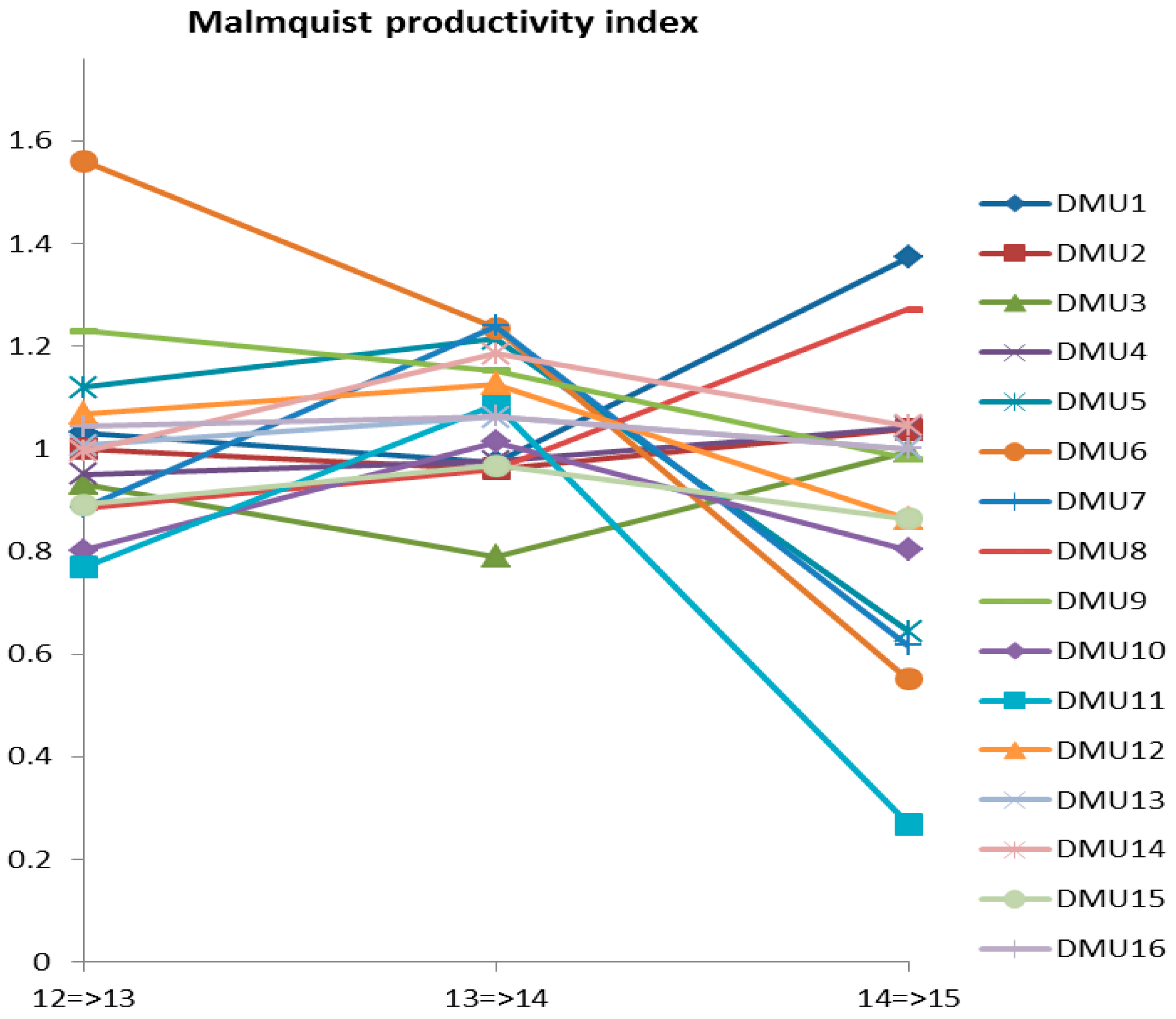
Table 7 lists the scores of efficiency change, technological change, and productivity change of the 16 GLPs from 2012 to 2015. Figure 2 shows that the efficiency change index of almost all of the DMUs are outstanding, with efficiency scores greater than 1, except for DMU2 (Werner Enterprises, Inc., Omaha, NE, USA), DMU7 (Con-way Freight, Ann Arbor, MI, USA), and DMU11 (CSX Corporation, Jacksonville, FL, USA), DMU1 (Ryder, Miami, FL, USA) comes in with a score of 1.019 and was the most efficient company on the efficiency change index.
Technical change is often considered in terms of “innovation” or “frontier-shift” effect measures. This can be compared across time by means of the Malmquist index. The improvement achieved mainly stems from the technical change (Frontier) that occurs. The efficiency change can also make a minor contribution to GLPs from 2012 to 2015. Technical change indicates a change in the technology index, which affects the relationship between inputs and outputs. The results show that during the period from 2012 to 2015 there were 13 companies that improved their level of input and achieved technical efficiency scores larger than 1. This indicates that the improvement of these companies is mainly attributable to technical improvement. DMU3 (Hub Group Inc., Downers Grove, IL, USA), DMU10 (Hyster-Yale Materials Handling Inc., Cleveland, OH, USA), and DMU15 (Swift Transportation Co., Phoenix, AZ, USA) are the top U.S. logistics firms. However, the operational performance of these three companies worsened because the scores for their technical and productivity changes dipped below 1, which indicates that they realized productivity loss and lower capital income. Thus, if these companies want to improve their MPIs, they should enhance their technical efficiency in the near future. The worse productivity shown in the period 2012–2015 came from weakened input of technical efficiency in most cases. DMU6 (United Parcel Service, Inc., Atlanta, GA, USA) had the highest productivity growth over the period 2012–2015, with a score of 1.158653147, while DMU11 (CSX Corporation, Jacksonville, FL, USA) showed the greatest loss. The results indicated that 10 of the DMUs, including DMU1 (Ryder, Miami, FL, USA), DMU4 (C.H. Robinson Worldwide, Inc., Eden Prairie, MN, USA), DMU5 (FedEx Corporation, Memphis, TN, USA), DMU6 (United Parcel Service, Inc. Atlanta, GA, USA), DMU8 (J.B. Hunt Transport Services, Inc., Lowell, AR, USA), DMU9 (Old Dominion Freight Line, Thomasville, NC, USA), DMU12 (Norfolk Southern Corp., Norfolk, VA, USA), DMU13 (Knight Transportation, Phoenix, AZ, USA), DMU14 (Union Pacific, Omaha, NE, USA), and DMU16 (Saia Inc., Johns Creek, GA, USA) showed productivity growth; the other six DMUs, namely DMU2 (Werner Enterprises, Omaha, NE, USA), DMU3 (Hub Group Inc., Downers Grove, IL, USA), DMU7 (Con-way Freight, Ann Arbor, MI, USA), DMU10 (Hyster-Yale Materials Handling, Cleveland, OH, USA), DMU11(CSX Corporation, Jacksonville, FL, USA), and DMU16 (Saia Inc., Johns Creek, GA, USA) showed relative productivity loss. The decrease in productivity in this period came from an evolution in the input technical efficiency achieved. Thus, these companies need to learn from more advanced logistics companies and thereby reinforce their organizational values to improve and reach the fittest scale of operating efficiency. Moreover, the main source of improvement will be technical efficiency change.
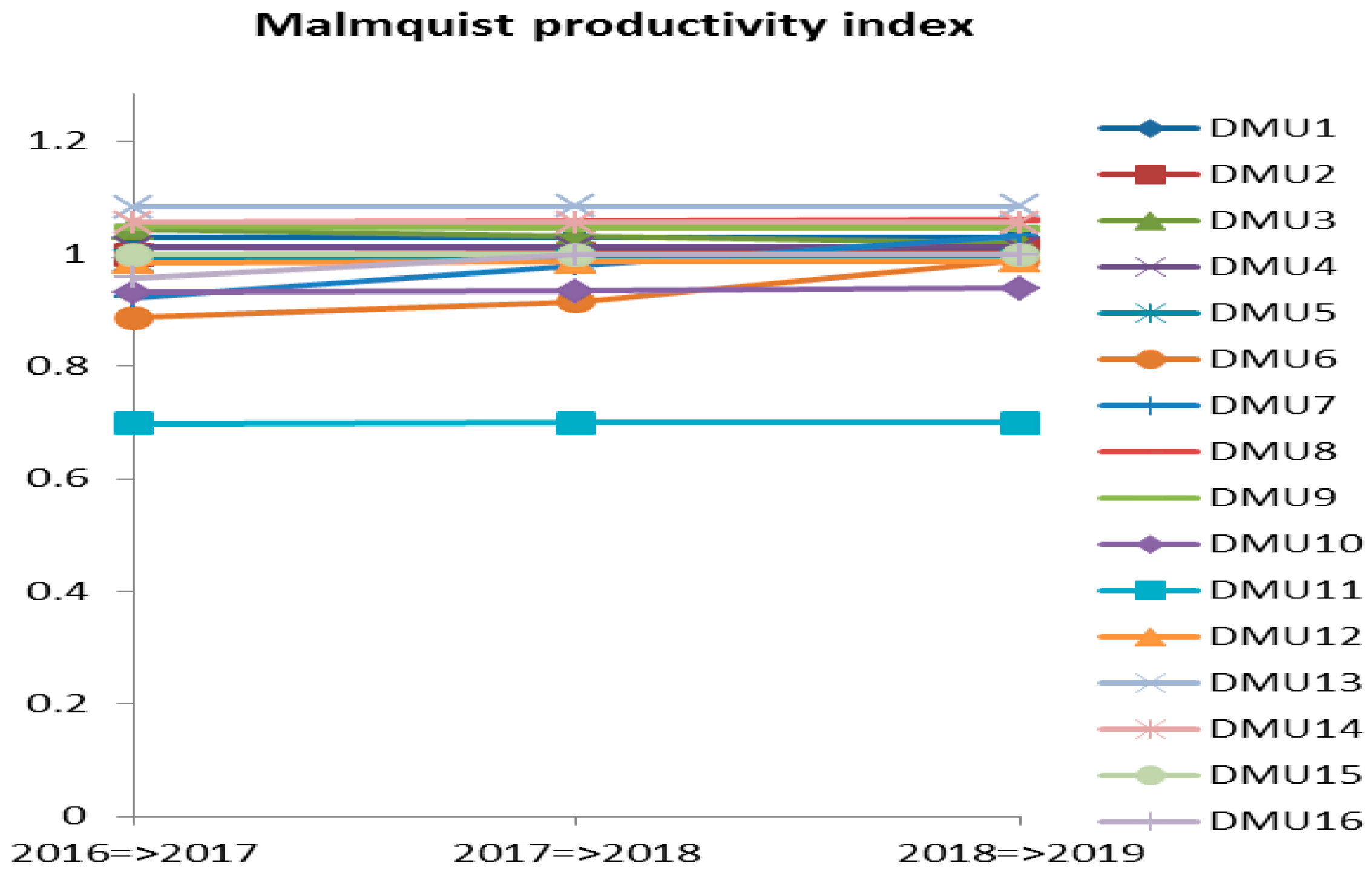
It is important to understand the differences between the past and the future of DMUs. Obviously, from Table 8 and Figure 3 we can see that almost all of the MPIs of companies reached “efficiency” in the period 2016–2019; however, the average of efficiency change is down by 0.57% and the average of technical change increased by 2.15% when compared to the previous year. In the future, the MPI of DMU1 (Ryder, Miami, FL, USA), DMU3 (Hub Group Inc., Downers Grove, IL, USA), DMU4 (C.H. Robinson Worldwide, Eden Prairie, MN, USA), DMU7 (Con-way Freight, Ann Arbor, MI, USA), DMU8 (J.B. Hunt Transport Services, Lowell, AR, USA), DMU9 (Old Dominion Freight Line, Thomasville, NC, USA), DMU13 (Knight Transportation, Phoenix, AZ, USA), and DMU14 (Union Pacific, Omaha, NE, USA) will perform well, all with a score larger than 1. Therefore, these companies are the best choice for purposes of cooperation. In contrast, DMU2 (Werner Enterprises, Omaha, NE, USA), DMU10 (Hyster-Yale Materials Handling, Cleveland, OH, USA), and DMU11 (CSX Corporation, Jacksonville, FL, USA) still maintain inefficient performance during the next four years. Thus, if a DMU wants to reach efficiency, it should follow an enterprise development strategy, prepare financial policies to improve the complete operation effect, and improve in terms of efficiency and technical changes.

5. Discussion

The U.S. logistics industry is highly competitive. Thus, American logistics companies need to secure ways to stand squarely in the competitive market. For instance, managers seek to cooperate with effective partners who have the financial performance capacity and consideration to protect the environment. However, how to identify preferred solutions that will balance business and environmental concerns is one of the most important questions in logistics today [61]. For this reason, this study assesses the economic performance of GLPs in order to select the most sustainable partners to achieve sustainable collaboration and to reduce environmental risk. To implement a valid and reliable evaluation process while addressing the various green U.S. logistics companies required us to integrate the grey GM (1,1) model and the DEA method to forecast and o analyze the given economic statements of the 16 selected GLPs in the period 2012–2019.
In particular, the analysis focuses on the forecasting results as well as the trends of technological progress and technical efficiency change among the companies. The principal findings are that, since the period of 2012–2015, the efficiency and productivity change of DMUs has been identified as “in regression” because the average change scores are 0.981 and 0.995. The findings of decreased productivity growth are related to technical change. Thus, the pressure on GLPs to improve their productivity gives more attention to sustainability in innovative activities and practices. Moreover, the performance of DMUs in the period 2016–2019 is identified as “progressive” because the average scores for technical and productivity change are 1.037 and 1.011. Again, this is noted as a decrease.
In summary, the results discussed in this study present a clear picture of the past, current and future situation of 16 green logistics companies in the USA. This study is based on the measures of change in technical efficiency, technological change, and MPI for each of the GLPs. It can be seen that there are two GLPs, Knight Transportation and Union Pacific Corporation, that reached their financial sustainability goals. The operational performance of these companies is measured in terms of efficiency among the 16 green logistics companies from the past to future. The less efficient firms, such as DMU10 (Hyster-Yale Materials Handling, Cleveland, OH, USA) and DMU11 (CSX Corporation, Jacksonville, FL, USA), should carry out efficiency change, technical change, and increase their ability to do more with less, as well as reduce wastage in terms of time, materials, and costs. According to the results, investors may wish to consider which companies are suitable for long-term cooperation based on the study results.

6. Conclusions

This study proposed an effective integrated method helpful to organizations that need to decide how to select their best sustainable development goals partner. The GM (1,1) is used as a method of predictive performance for the period 2016–2019. The DEA models are used as a tool to rank and measure the performance of GLPs’ financial situation in the period 2012–2019. Finally, the study provides useful knowledge about economic efficiency in the general management of the GLPs. This research supports the corporate selection process with regards to sustainable development. In particular, it may help GLPs to understand their business status in the past, present, and near future. The empirical evidence of this research also gives meaningful suggestions for GLPs to better improve their profit, technology, scale efficiencies, and long-term plans. Thus, it has become important to measure DMUs’ economic sustainability performance as well as organizational operations. The limitation of the research is in the number of inputs and outputs that are considered relevant to financial results. Another limitation is how current the data are, specifically our four-year data. The results can be improved with longitudinal data. The number of GLPs available for analysis is 16. Research is needed to examine how green logistics providers can improve financial performance as well as environmental activities.
Any further study should include other factors covering environmental performance indicators to evaluate the environmental impact for the selection of environmentally sound practices and green technology.
From a researcher’s point of view, it is hoped that the integration of the models and techniques proposed in this study can be applied to diverse industries with similar plant structures to evaluate operational efficiency and determine appropriate and realistic means for improvement.

Acknowledgments

This research was supported by MOST 105-2221-E-151-039 and MOST 105-2622-E-151-006-CC3 from the Ministry of Sciences and Technology in Taiwan. The authors also appreciate the support from National Kaohsiung University of Applied Sciences and Fortune Institute of Technology.

Author Contributions

Chia-Nan Wang contributed to design the theoretical verifications and reviewed the manuscript. Hong-Xuyen Thi Ho was involved in writing and analyzing data. Shih-Hsiung Luo did the literature review and designed the framework. Tsung-Fu Lin edited and prepared the manuscript.

Conflicts of Interest

The authors declare no conflict of interest.

Abbreviations

The following abbreviations are used in this manuscript:
DEAData development analysis
DMUDecision-making unit
GM (1,1) Grey model (1,1)
SBMSlacks-based model
MAPEMean absolute percent error
GLPsGreen logistics providers

References

  1. Li, D.; Hanafi, Z. A Study of Eco-Performance of Logistics Services in Food Supply Chains; Springer: Berlin/Heidelberg, Germany, 2012; pp. 223–228. [Google Scholar]
  2. US Environmental Protection Agency. Sources of Greenhouse Gas Emissions. Available online: https://www.epa.gov/ghgemissions/sources-greenhouse-gas-emissions (accessed on 31 January 2017).
  3. Delivering Tomorrow: Towards Sustainable Logistics: How Business Innovation and Green Demand Drive a Carbon-Efficient Industry. Dt. Post, Konzernzentrale, 2008–2009. Available online: http://www.dhl-usa.com/content/dam/downloads/g0/logistics/green_logistics_sustainable_logistics_study_en.pdf (accessed on 31 January 2017).
  4. Sweeney, E.; Evangelista, P.; Huge-Brodin, M.; Isaksson, K. The role of third party logistics providers (3PLs) in the adoption of green supply chain initiatives. Dublin Inst. Technol. 2013, 84, 32–34. [Google Scholar]
  5. Seroka-Stolka, O. The development of green logistics for implementation sustainable development strategy in companies. Proced. Soc. Behav. Sci. 2014, 151, 302–309. [Google Scholar] [CrossRef]
  6. Presley, A.; Meade, L.; Sarkis, J. A strategic sustainability justification methodology for organizational decisions: A reverse logistics illustration. Int. J. Prod. Res. 2007, 45, 4595–4620. [Google Scholar] [CrossRef]
  7. Colicchia, C.; Marchet, G.; Melacini, M.; Perotti, S. Building environmental sustainability: Empirical evidence from Logistics Service Providers. J. Clean. Prod. 2013, 59, 197–209. [Google Scholar] [CrossRef]
  8. Abbasi, M.; Nilsson, F. Developing environmentally sustainable logistics: Exploring themes and challenges from a logistics service providers’ perspective. Transp. Res. Part D 2016, 46, 273–283. [Google Scholar]
  9. Van Marrewijk, M.; Werre, M. Multiple levels of corporate sustainability. J. Bus. Ethics 2003, 44, 107–119. [Google Scholar] [CrossRef]
  10. Tamulis, V.; Guzavičius, A.; Žalgirytė, L. Factors influencing the use of green logistics: Theoretical implications. Econ. Manag. 2012, 17, 706–711. [Google Scholar] [CrossRef]
  11. Sbihi, A.; Eglese, R.W. Combinatorial optimization and green logistics. Q. J. Oper. Res. 2007, 5, 99–116. [Google Scholar] [CrossRef] [Green Version]
  12. Chunguang, Q.; Xiaojuan, C.; Kexi, W.; Pan, P. Research on green logistics and sustainable development. In Proceedings of the 2008 IEEE International Conference on Information Management, Innovation Management and Industrial Engineering (ICIII), Taipei, Taiwan, 19–21 December 2008.
  13. Murphy, P.R.; Poist, R.F. Green perspectives and practices: A “comparative logistics” study. Supply Chain Manag. Int. J. 2003, 8, 122–131. [Google Scholar] [CrossRef]
  14. Lee, S.Y.; Klassen, R.D. Drivers and enablers that foster environmental management capabilities in small-and medium-sized suppliers in supply chains. Prod. Operat. Manag. 2008, 17, 573–586. [Google Scholar] [CrossRef]
  15. Wu, H.J.; Dunn, S.C. Environmentally responsible logistics systems. Int. J. Phys. Distrib. Logist. Manag. 1995, 25, 20–38. [Google Scholar] [CrossRef]
  16. Doane, D.; MacGillivray, A. Economic Sustainability: The business of staying in business. New Econ. Found. 2001, 1, 1–52. [Google Scholar]
  17. Kannan, D.; Khodaverdi, R.; Olfat, L.; Jafarian, A.; Diabat, A. Integrated fuzzy multi criteria decision making method and multi-objective programming approach for supplier selection and order allocation in a green supply chain. J. Clean. Prod. 2013, 47, 355–367. [Google Scholar] [CrossRef]
  18. Grisi, R.M.; Guerra, L.; Naviglio, G. Supplier performance evaluation for green supply chain management. Bus. Perform. Meas. Manag. 2010, 4, 149–163. [Google Scholar]
  19. Bhattacharya, A.; Mohapatra, P.; Kumar, V.; Dey, P.K.; Brady, M.; Tiwari, M.K.; Nudurupati, S.S. Green supply chain performance measurement using fuzzy ANP-based balanced scorecard: A collaborative decision-making approach. Prod. Plan. Control 2014, 25, 698–714. [Google Scholar] [CrossRef]
  20. Tarofder, A.K.; Haque, A. Exploring critical factors for supplier selection in telecommunication industry in Malaysia. Asian J. Mark. 2007, 1, 1–13. [Google Scholar] [CrossRef]
  21. Rao, P.; Holt, D. Do green supply chains lead to competitiveness and economic performance. Int. J. Oper. Prod. Manag. 2005, 25, 898–916. [Google Scholar] [CrossRef]
  22. Hervani, A.A.; Helms, M.M.; Sarkis, J. Performance measurement for green supply chain management. Benchmarking Int. J. 2005, 12, 330–353. [Google Scholar] [CrossRef]
  23. Tsai, W.H.; Hung, S.J. A fuzzy goal programming approach for green supply chain optimization under activity-based costing and performance evaluation with a value-chain structure. Int. J. Prod. Res. 2009, 47, 4991–5017. [Google Scholar] [CrossRef]
  24. Chung, C.C.; Chao, L.C.; Lou, S.J. The Establishment of a Green Supplier Selection and Guidance Mechanism with the ANP and IPA. Sustainability 2016, 8, 259. [Google Scholar] [CrossRef]
  25. Fowler, S.J.; Hope, C. A critical review of sustainable business indices and their impact. J. Bus. Ethics 2007, 76, 243–256. [Google Scholar] [CrossRef]
  26. Lee, K.H.; Kim, J.W. Integrating suppliers into green product innovation development: An empirical case study in the semiconductor industry. Bus. Strateg. Environ. 2011, 20, 527–538. [Google Scholar] [CrossRef]
  27. JuLong, D. Control problems of grey systems. Syst. Control Lett. 1982, 1, 288–294. [Google Scholar] [CrossRef]
  28. Li, L.; Lei, Y.; Zhao, L.; Li, X. Study on the Optimization of the Industrial Structure in a Mining Economic Region: Taking Carbon Emissions as a Restriction. Minerals 2015, 5, 203–220. [Google Scholar] [CrossRef]
  29. Wen, Y.H. Shipment forecasting for supply chain collaborative transportation management using grey models with grey numbers. Transp. Plan. Technol. 2011, 34, 605–624. [Google Scholar] [CrossRef]
  30. Li, C.B.; Wang, K.C. A new grey forecasting model based on BP neural network and Markov chain. J. Cent. South Univ. Technol. 2007, 14, 713–718. [Google Scholar] [CrossRef]
  31. Geng, N.; Zhang, Y.; Sun, Y.; Jiang, Y.; Chen, D. Forecasting China’s Annual Biofuel Production Using an Improved Grey Model. Energies 2015, 8, 12080–12099. [Google Scholar] [CrossRef]
  32. Wu, H.H.; Liao, A.Y.H.; Wang, P.C. Using grey theory in quality function deployment to analyze dynamic customer requirements. Int. J. Adv. Manuf. Technol. 2005, 25, 1241–1247. [Google Scholar] [CrossRef]
  33. Huang, Y.F.; Wang, C.N.; Dang, H.S.; Lai, S.T. Predicting the trend of Taiwan’s electronic paper industry by an effective combined grey model. Sustainability 2015, 7, 10664–10683. [Google Scholar] [CrossRef]
  34. Cooper, W.W.; Seiforf, L.M.; Zhu, J. Data envelopment analysis: History, models, and interpretations. In Handbook on Data Envelopment Analysis; Springer: Berlin/Heidelberg, Germany, 2004; pp. 1–39. [Google Scholar]
  35. Wang, D.; Li, S.; Sueyoshi, T. DEA environmental assessment on US Industrial sectors: Investment for improvement in operational and environmental performance to attain corporate sustainability. Energy Econ. 2014, 45, 254–267. [Google Scholar] [CrossRef]
  36. Zhou, G.; Min, H.; Xu, C.; Cao, Z. Evaluating the comparative efficiency of Chinese third-party logistics providers using data envelopment analysis. Int. J. Phys. Distrib. Logist. Manag. 2008, 38, 262–279. [Google Scholar] [CrossRef]
  37. Hamdan, A.; Rogers, K.J. Evaluating the efficiency of 3PL logistics operations. Int. J. Prod. Econ. 2008, 113, 235–244. [Google Scholar] [CrossRef]
  38. Ramanathan, R. Supplier selection problem: Integrating DEA with the approaches of total cost of ownership and AHP. Suppl. Chain Manag. Int. J. 2007, 12, 258–261. [Google Scholar] [CrossRef]
  39. Saen, R.F. A new model for selecting third-party reverse logistics providers in the presence of multiple dual-role factors. Int. J. Adv. Manuf. Technol. 2010, 46, 405–410. [Google Scholar] [CrossRef]
  40. Azadi, M.; Saen, R.F. A new chance-constrained data envelopment analysis for selecting third-party reverse logistics providers in the existence of dual-role factors. Expert Syst. Appl. 2011, 38, 12231–12236. [Google Scholar] [CrossRef]
  41. Guarnieri, P.; Sobreiro, V.A.; Nagano, M.S.; Serrano, A.L.M. The challenge of selecting and evaluating third-party reverse logistics providers in a multicriteria perspective: A Brazilian case. J. Clean. Prod. 2015, 96, 209–219. [Google Scholar] [CrossRef]
  42. Singhal, K.; Singhal, J. Imperatives of the science of operations and supply-chain management. J. Oper. Manag. 2012, 30, 237–244. [Google Scholar] [CrossRef]
  43. Marschall, P.; Flessa, S. Assessing the efficiency of rural health centres in Burkina Faso: An application of Data Envelopment Analysis. J. Public Healt. 2009, 17, 87–95. [Google Scholar] [CrossRef]
  44. Sun, L.; Stuebs, M. Corporate social responsibility and firm productivity: Evidence from the chemical industry in the United States. J. Bus. Ethics 2013, 118, 251–263. [Google Scholar] [CrossRef]
  45. Lin, W.; Chen, B.; Xie, L.; Pan, H. Estimating energy consumption of transport modes in China using DEA. Sustainability 2015, 7, 4225–4239. [Google Scholar] [CrossRef]
  46. Kuo, R.J.; Wang, Y.C.; Tien, F.C. Integration of artificial neural network and MADA methods for green supplier selection. J. Clean. Prod. 2010, 18, 1161–1170. [Google Scholar] [CrossRef]
  47. Lo, S.F.; Lu, W.M. An integrated performance evaluation of financial holding companies in Taiwan. Eur. J. Oper. Res. 2009, 198, 341–350. [Google Scholar] [CrossRef]
  48. Pang, J.; Chen, X.; Zhang, Z.; Li, H. Measuring Eco-Efficiency of Agriculture in China. Sustainability 2016, 8, 398. [Google Scholar] [CrossRef]
  49. Marchet, G.; Melacini, M.; Sassi, C.; Tappia, E. Assessing Efficiency and Innovation in the 3PL Industry: An Empirical Analysis. Available online: http://dx.doi.org/10.1080/13675567.2016.1226789 (accessed on 31 January 2017).
  50. Shuai, J.J.; Wu, W.W. Evaluating the influence of E-marketing on hotel performance by DEA and grey entropy. Expert Syst. Appl. 2011, 38, 8763–8769. [Google Scholar] [CrossRef]
  51. Liu, J.L.; Wang, M.D.; Bai, Y. Using DEA and Grey Markovian Model to Measure the Goal Cost of Petroleum Enterprise. In Proceedings of the International Conference on Computational Science, Beijing, China, 27–30 May 2007.
  52. Wang, C.N.; Nguyen, N.T.; Tran, T.T. Integrated DEA models and grey system theory to evaluate past-to-future performance: A case of Indian electricity industry. Sci. World J. 2015, 2015, 1–17. [Google Scholar]
  53. Chen, Y.S.; Chen, B.Y. Applying DEA, MPI, and grey model to explore the operation performance of the Taiwanese wafer fabrication industry. Technol. Forecast. Soc. Chang. 2011, 78, 536–546. [Google Scholar] [CrossRef]
  54. Inbound Logistics’ 75 Green Supply Chain Partners. Available online: http://www.inboundlogistics.com/cms/article/g75-inbound-logistics-75-green-supply-chain-partners/ (accessed on 31 January 2017).
  55. Google Finance. Available online: https://www.google.com/finance (accessed on 1 February 2017).
  56. Tone, K. A slacks-based measure of efficiency in data envelopment analysis. Eur. J. Oper. Res. 2001, 130, 498–509. [Google Scholar] [CrossRef]
  57. Zhu, J. Quantitative Models for Performance Evaluation and Benchmarking: Data Envelopment Analysis with Spreadsheets; Springer: Berlin/Heidelberg, Germany, 2014; pp. 11–48. [Google Scholar]
  58. Logistics and Supply Chain Management Consulting. Available online: http://www.ltdmgmt.com/AccountingCosts.php (accessed on 31 January 2017).
  59. Tone, K. A slacks-based measure of super-efficiency in data envelopment analysis. Eur. J. Oper. Res. 2002, 143, 32–41. [Google Scholar] [CrossRef]
  60. Andersen, P.; Petersen, N.C. A procedure for ranking efficient units in data envelopment analysis. Manag. Sci. 1993, 39, 1261–1264. [Google Scholar] [CrossRef]
  61. Quariguasi Frota Neto, J.; Bloemhof-Ruwaard, J.M. The Environmental Gains of Remanufacturing: Evidence from the Computer and Mobile Industry; Erasmus Research Institute of Management: Rotterdam, The Netherlands, 2009; pp. 1–31. [Google Scholar]
Figure 1. Process of proposed method.
Sustainability 09 00218 g001
Figure 2. Productivity index (MPI) change over the period 2012–2015.
Sustainability 09 00218 g002
Figure 3. Productivity index (MPI) change over the period 2016–2019.
Sustainability 09 00218 g003
Table 1. Input/output value of DMU2 from 2012 to 2015 (in millions of U.S. dollars).
Years(I) Total Assets(I) Total Operating Expense(I) Total Current Liabilities(I) Total Equity(O) EPS(O) Net Income(O) Total Revenue
20121334.901864.94176.19714.91.4103.032036.39
20131354.101889.46167.73772.521.1886.782029.18
20141480.461979.20186.53833.861.3698.652139.29
20151613.681893.07183.7935.651.71123.712093.53
Table 2. The actual value (2012–2015) and the forecasting value (2016–2019) of DMU2.
Years(I) Total Assets(I) Total Operating Expense(I) Total Current Liabilities(I) Total Equity(O) EPS(O) Net Income(O) Total Revenue
20121334.901864.94176.19714.91.4103.032036.39
20131354.101889.46167.73772.521.1886.782029.18
20141480.461979.20186.53833.861.3698.652139.29
20151613.681893.07183.7935.651.71123.712093.53
20161760.701924.13195.521024.472.04146.232151.66
20171921.791925.92204.241128.782.47175.522184.67
20182097.611927.70213.351243.702.98210.672218.18
20192289.531929.49222.871370.323.61252.872252.21
Table 3. Predicted values of outputs for all DMUs from 2016 to 2019.
DMUsOutputs (Millions of U.S. Dollars, Except EPS)
2016201720182019
(O) EPS(O) Net Income(O) Total Revenue(O) EPS(O) Net Income(O) Total Revenue(O) EPS(O) Net Income(O) Total Revenue(O) EPS(O) Net Income(O) Total Revenue
DMU16.11333.426696.226.8986384.096774.207.788442.466853.098.7911509.76932.889
DMU22.0389146.232151.662.4663175.522184.72.983210.672218.23.6085252.92252.211
DMU31.8665.9293642.721.919966.9863721.81.98268.0593802.62.045669.153885.191
DMU44.0297560.9113,965.84.6366621.8914,3505.335689.4914,7446.1385764.415,149.16
DMU53.7061269.249,029.32.94641117.450,7582.343983.752,5491.862486654,401.85
DMU61.0598944.5518,338.80.6465564.9212,3040.394337.878255.30.2405202.15538.805
DMU70.985357.5041843.790.775245.4521243.70.6135.926838.880.479828.4565.8379
DMU84.1071474.726596.674.6469531.036932.45.258594.027285.35.9485664.57656.077
DMU94.3665371.243382.225.2918447.363796.56.413539.094261.57.7723649.64783.492
DMU104.265369.2662585.033.64458.4862543.43.11349.3842502.52.659841.72462.262
DMU110.6333621.253908.370.4315418.482605.80.294281.891737.40.2004189.91158.336
DMU125.00831509.410,427.24.64171376.110,0964.3021254.59775.83.987111449465.468
DMU131.8229151.191313.492.2936191.621448.22.886242.861596.73.6308307.81760.488
DMU146.10885159.922,442.96.55465362.722,3717.0335573.322,2997.5459579222,227.18
DMU151.5256219.164326.591.7287248.734383.41.959282.344412.2196320.44499.365
DMU161.326862.4131293.221.179669.7621336.71.04977.9771381.70.932387.161428.232
Table 4. Average MAPE of DMUs.
DMUsAverage MAPEDMUsAverage MAPE
DMU120%DMU91%
DMU21%DMU102%
DMU321%DMU1111%
DMU42%DMU123%
DMU57%DMU134%
DMU614%DMU142%
DMU716%DMU152%
DMU82%DMU163%
Average of all MAPEs: 7%
Table 5. Scores and rankings of GLPs in 2012–2015.
DMUs2012201320142015
ScoreRankScoreRankScoreRankScoreRank
DMU10.488863150.4916803150.5025056151.078495510
DMU21.0002291141.0109913131.0170784120.799280114
DMU31.0826904102.074452411.0268109101.020946412
DMU41.492565721.281968761.271518661.39473433
DMU51.289021261.1166866101.240221871.25011866
DMU61.277872471.898609422.037784811.15517969
DMU70.4422939160.4155573160.5445534140.246516515
DMU81.102311191.0113463121.0181149111.1630588
DMU91.0392105111.149869991.192336581.20409837
DMU101.365100131.304766951.288904751.31702114
DMU111.0071753130.506942140.4761674160.7516
DMU121.0194534121.0152636111.0167316131.00253471513
DMU131.623360611.475219231.315088941.4219509852
DMU141.297965151.232527771.330641331.5366603261
DMU151.261429381.220587181.073924191.05976166211
DMU161.356465141.311689241.405506821.3008117765
Table 6. Future scores and ranking of GLPs in 2016–2019.
DMUs2016201720182019
ScoreRankScoreRankScoreRankScoreRank
DMU11.08615981.07169231781.057029291.04133128
DMU20.4001969110.527254787132.9795169119.482931211
DMU30.999878490.152763789104.23012791226.14114314
DMU41.381743521.40379144521.410019421.373743
DMU51.25180241.25767525361.263435361.26908356
DMU60.1749859120.04188681110.4350099101.394133210
DMU70.1185371140.99838581391.205614181.49383362
DMU80.8245403100.176786361125.19204371427.65864715
DMU91.203087561.26203133751.28049851.30250094
DMU101.263256431.2801275431.297813341.27550215
DMU110.8543239164.4941446571617.1211881662.01007816
DMU120.1030013151.485976223156.983836315–25.9245113
DMU131.202366371.19442820671.207140571.22934347
DMU141.659584211.78725016911.763036111.75301091
DMU150.1602937131.05740333814–4.3451181312.77076912
DMU161.223168551.26285796241.315618330.99974759
Table 7. GLPs’ average productivity changes during 2012–2015.
DMUsEfficiency Change Index (Catch-up)Technical Change Index (Frontier)Productivity Index (Malmquist-MPI)
DMU11.019150361.0108185731.02119458
DMU20.9860333761.0008112280.986164214
DMU310.9613927580.961392758
DMU411.0017927521.001792752
DMU511.0206298351.020629835
DMU611.1586531471.158653147
DMU70.9669424351.0090053440.962756457
DMU811.0042139591.004213959
DMU911.0913864651.091386465
DMU1010.8508180240.850818024
DMU110.7278110711.0230398080.747250075
DMU1211.0101101441.010110144
DMU1311.0403968181.040396818
DMU1411.0346789521.034678952
DMU1510.963335840.96333584
DMU160.9999999461.0782356741.078235632
Average0.9812460741.0162074580.995813103
Max1.019150361.1586531471.158653147
Min0.7278110710.8508180240.747250075
SD0.0683686390.0656471380.094426774
Table 8. GLPs’ average productivity changes during 2016–2019.
DMUsEfficiency Change Index (Catch-up)Technical Change Index (Frontier)Productivity Index (Malmquist-MPI)
DMU111.0733020871.073302087
DMU20.995617540.9987902330.994412322
DMU311.0977807651.097780765
DMU411.0388583011.038858301
DMU510.9925025040.992502504
DMU60.9144002981.0128894150.926878278
DMU71.0810352331.0250363921.100557137
DMU811.0692420681.069242068
DMU911.0977559291.097755929
DMU1010.9802896850.980289685
DMU110.67523291.0364840520.699868249
DMU120.945051381.0385008790.981294432
DMU1311.0888988091.088898809
DMU1411.0530782921.053078292
DMU150.9959480531.0018572870.997795949
DMU160.9999996780.9982723780.998272056
Average0.9754553181.0377211921.011924179
Max1.0810352331.0977807651.100557137
Min0.67523290.9802896850.699868249
SD0.0867116290.0389940040.098526314

