
Evaluation of Sulfide Control by Air-Injection in Sewer Force Mains: Field and Laboratory Study


Abstract
:1. Introduction
2. Experimental Setting
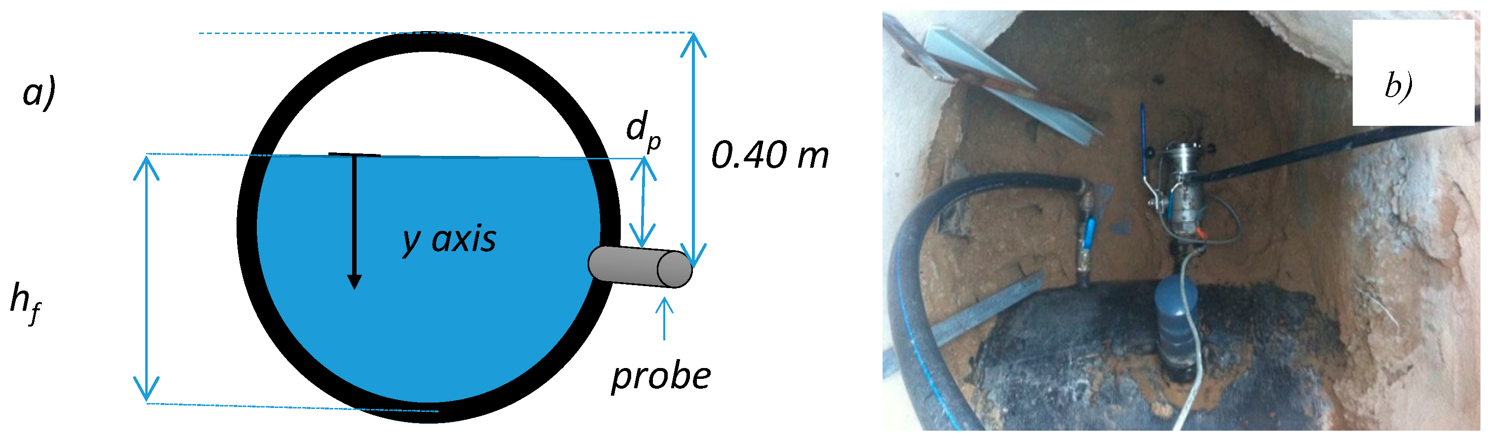
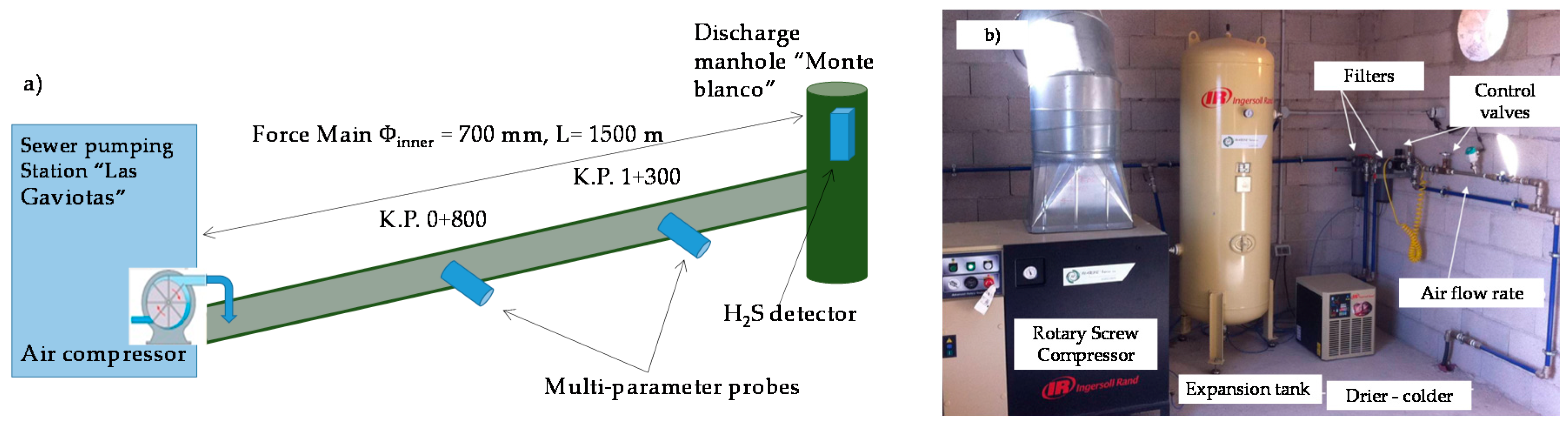
2.1. Sewer Pumping Station
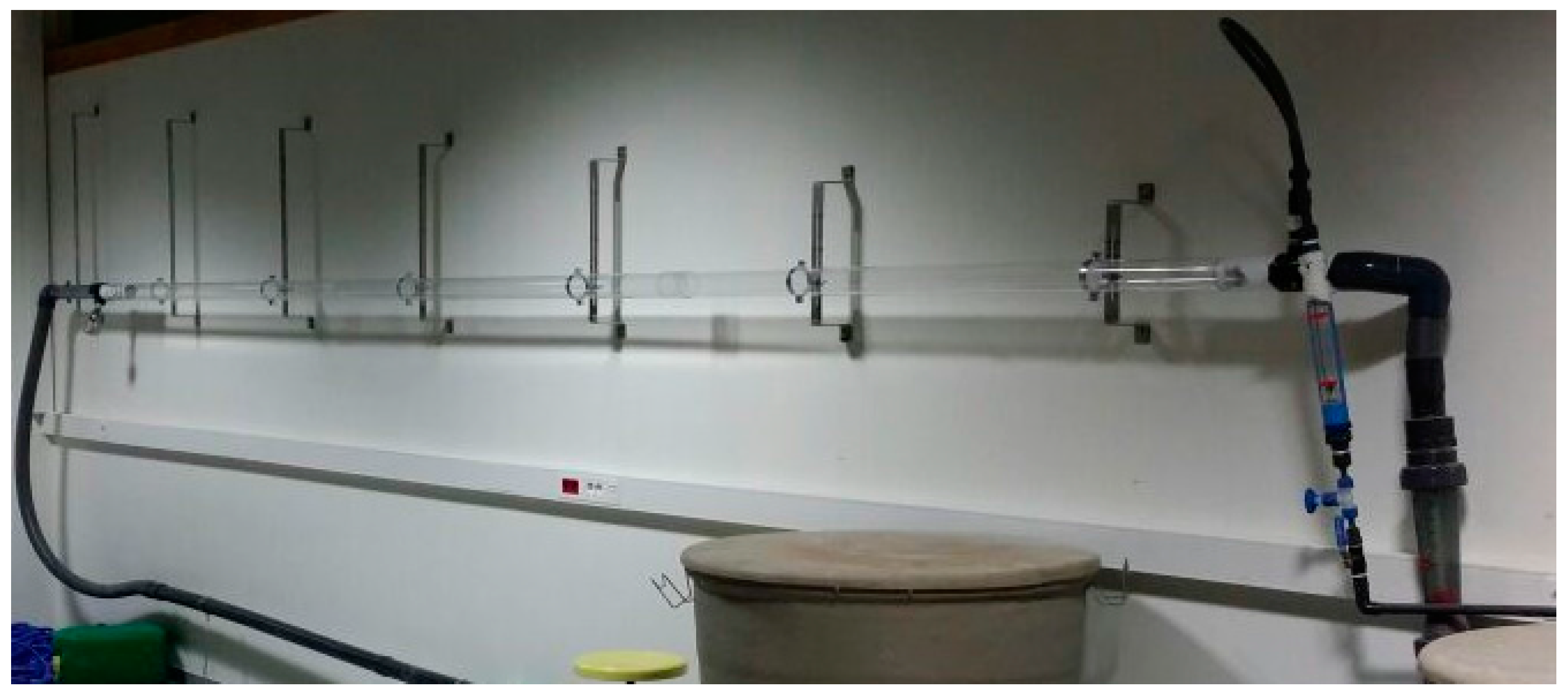
2.2. Laboratory Scale Model
3. Results and Discussion
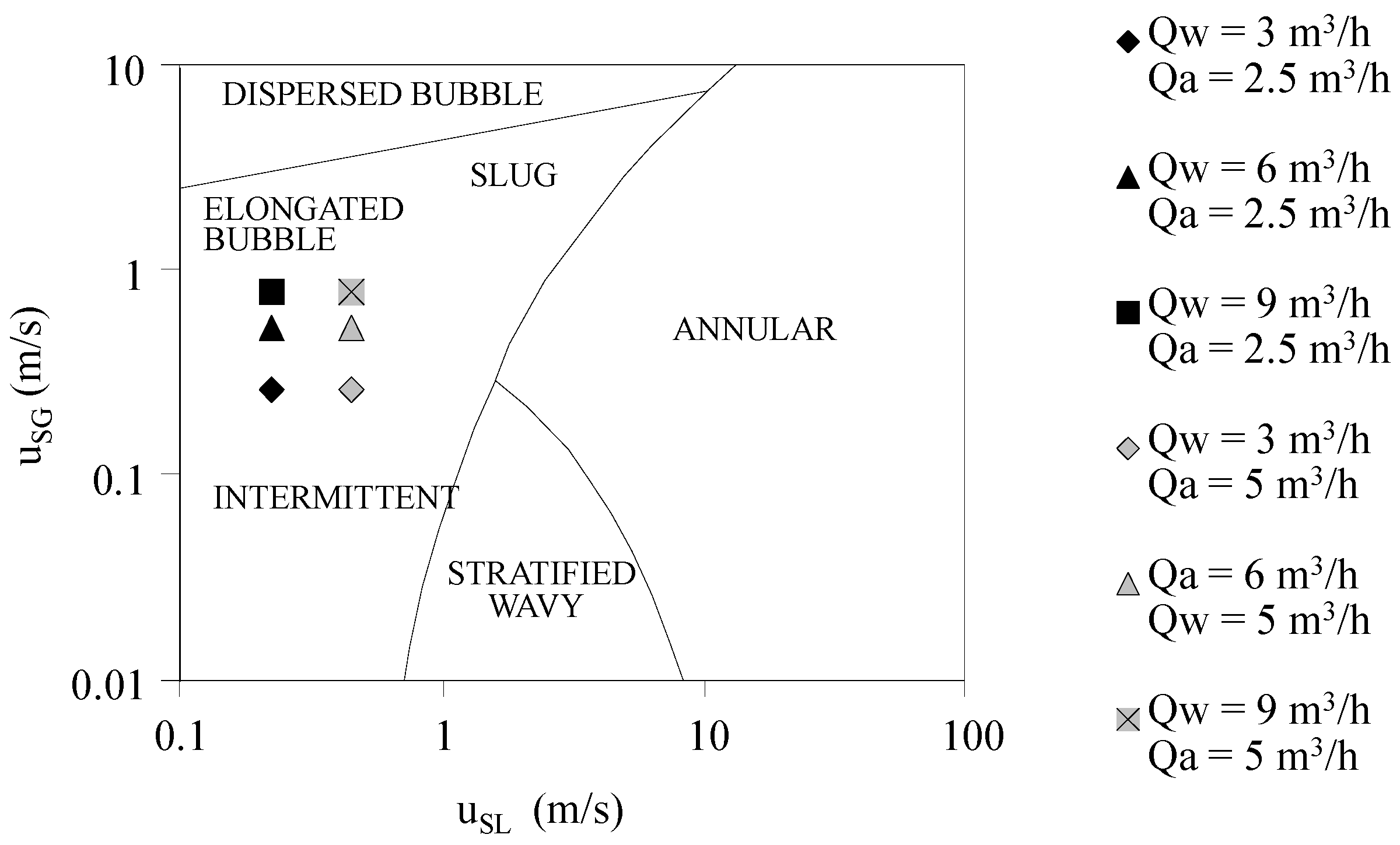
3.1. Laboratory Scale Model
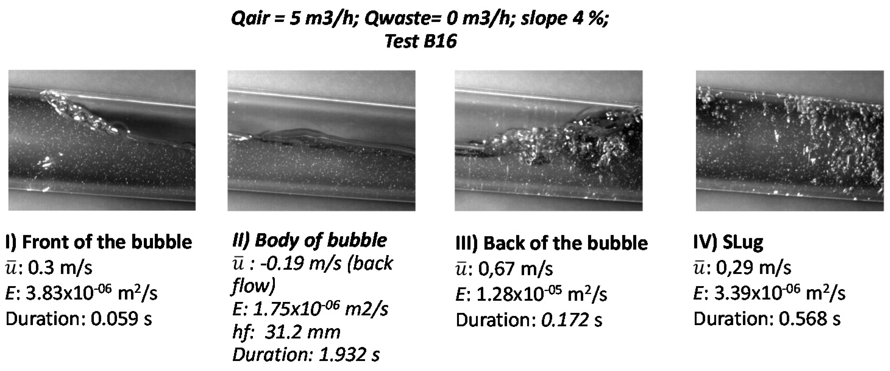
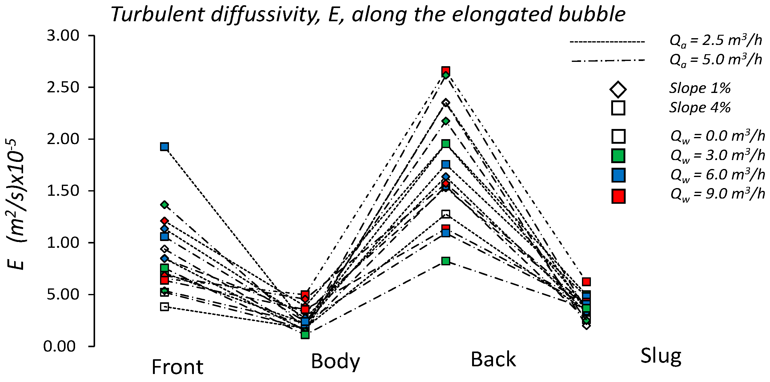
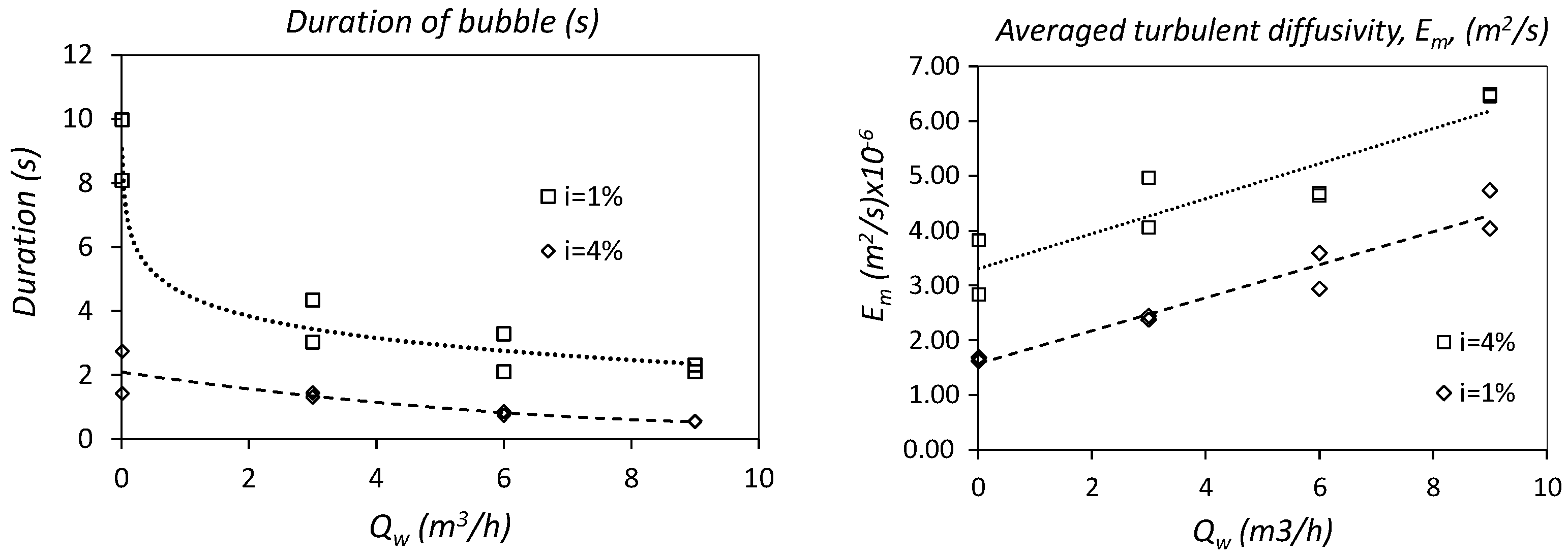
3.1.1. Velocity Field of Water Phase and Turbulent Diffusivity
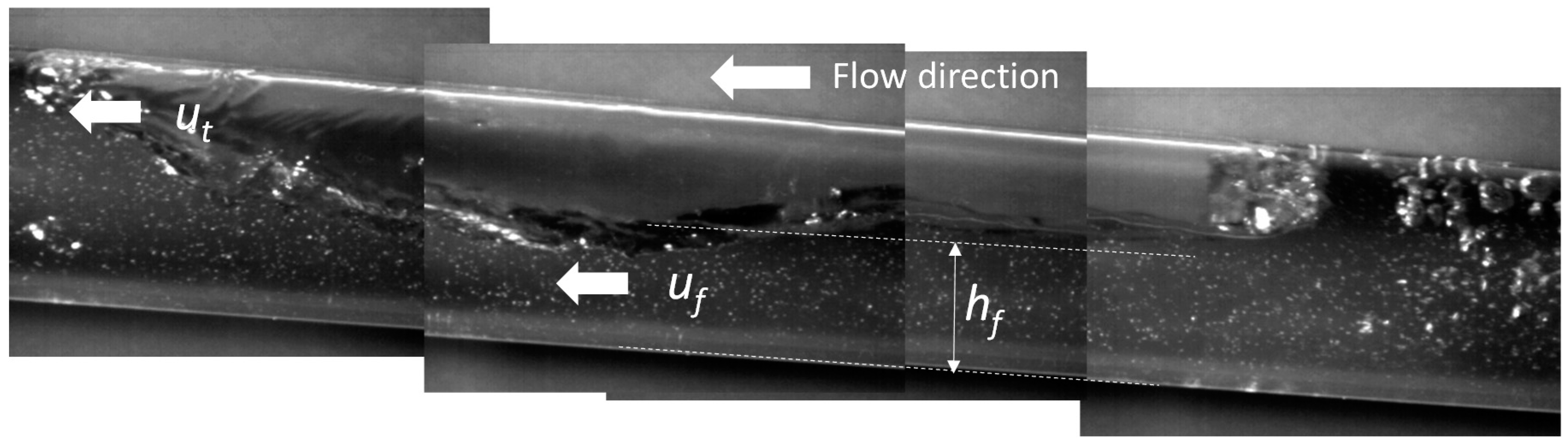
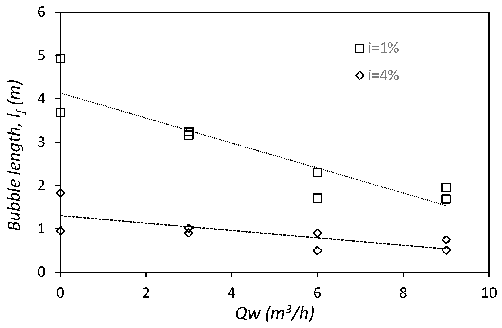
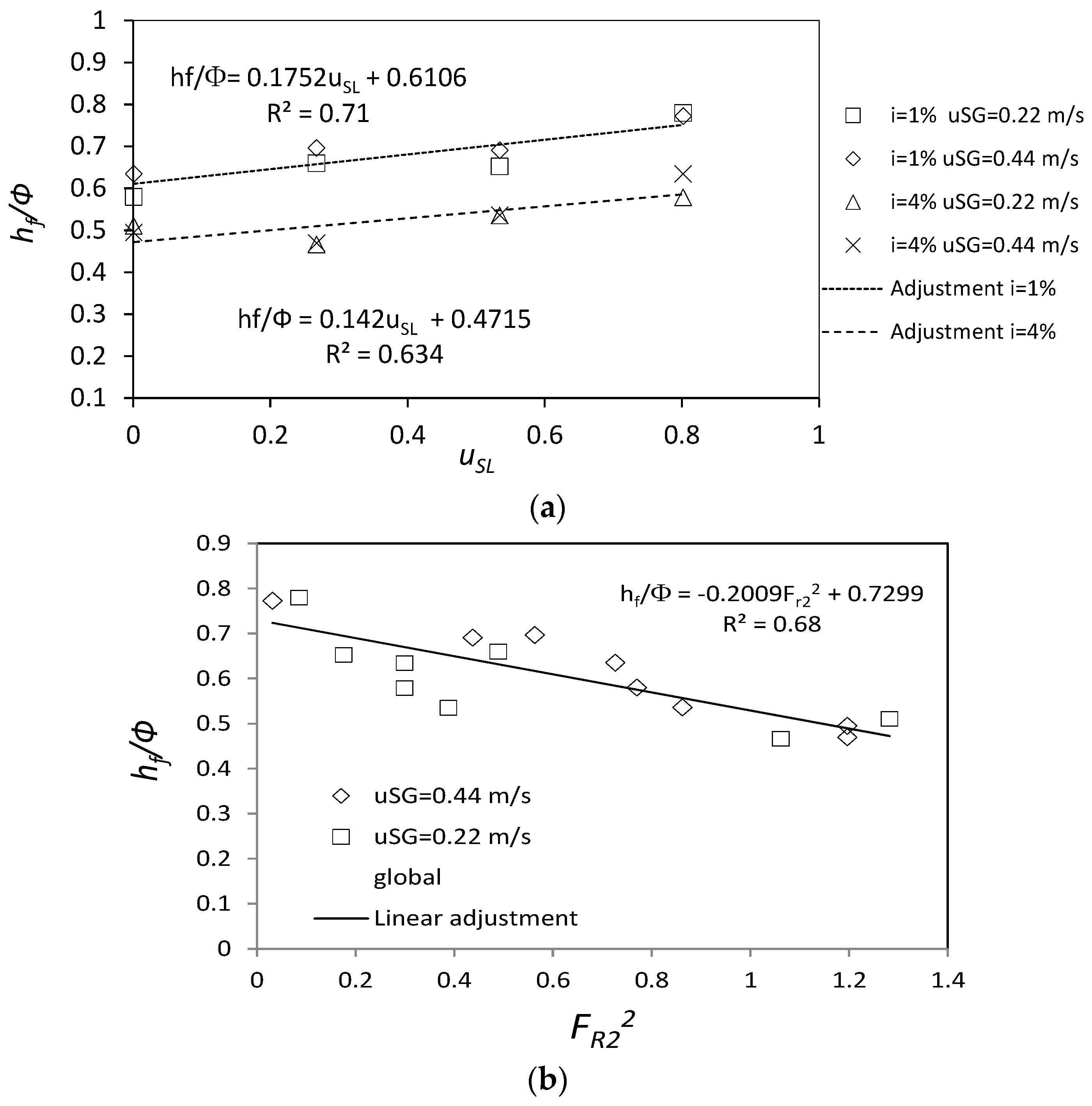
3.1.2. Flow Depth in the Body of the Bubble, hf
3.1.3. Linear Regression of the Turbulent Diffusion, Em
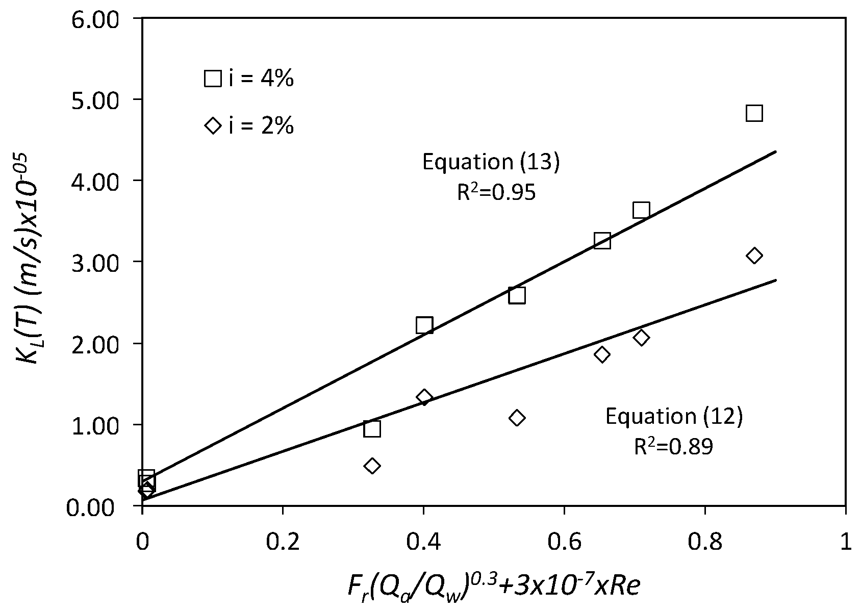
3.1.4. Mass Transfer Coefficient at the Air–Water Inter-Phase, KL(T)
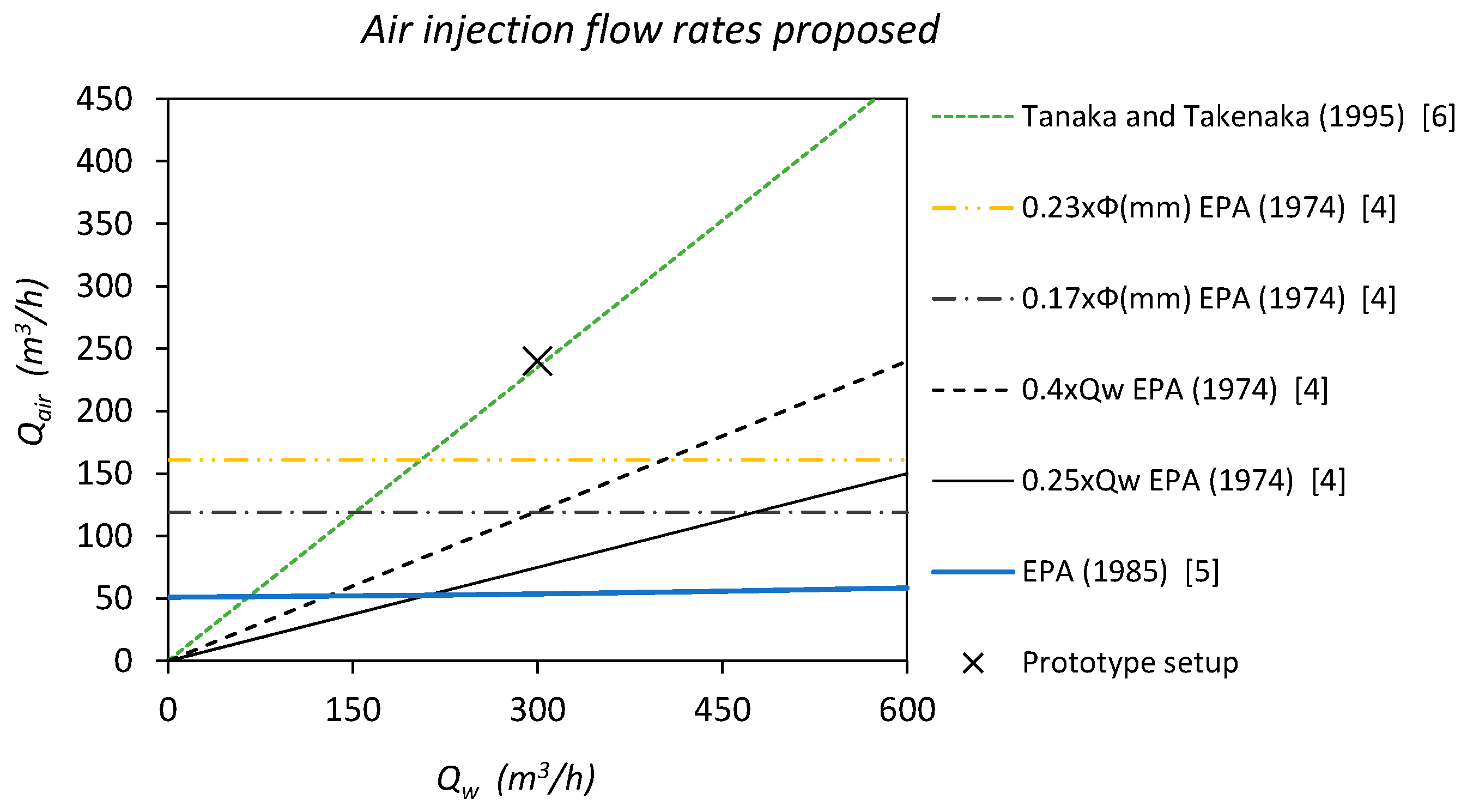
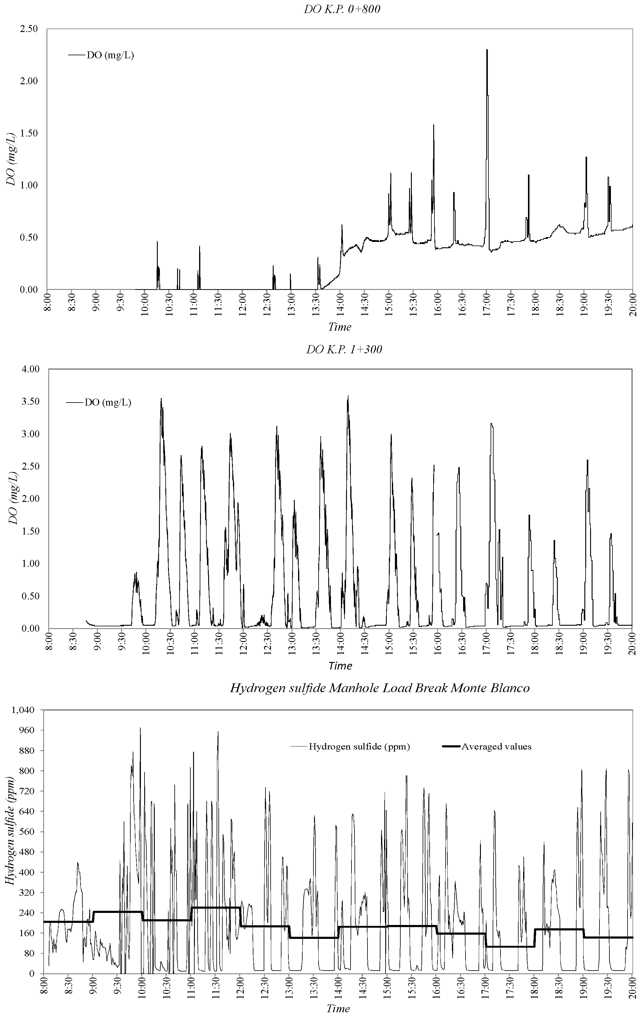
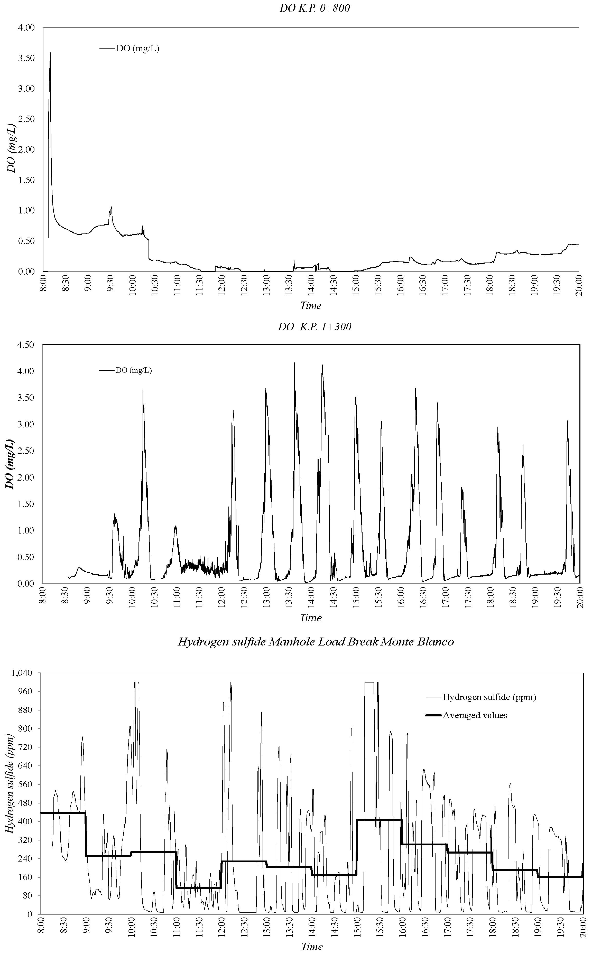
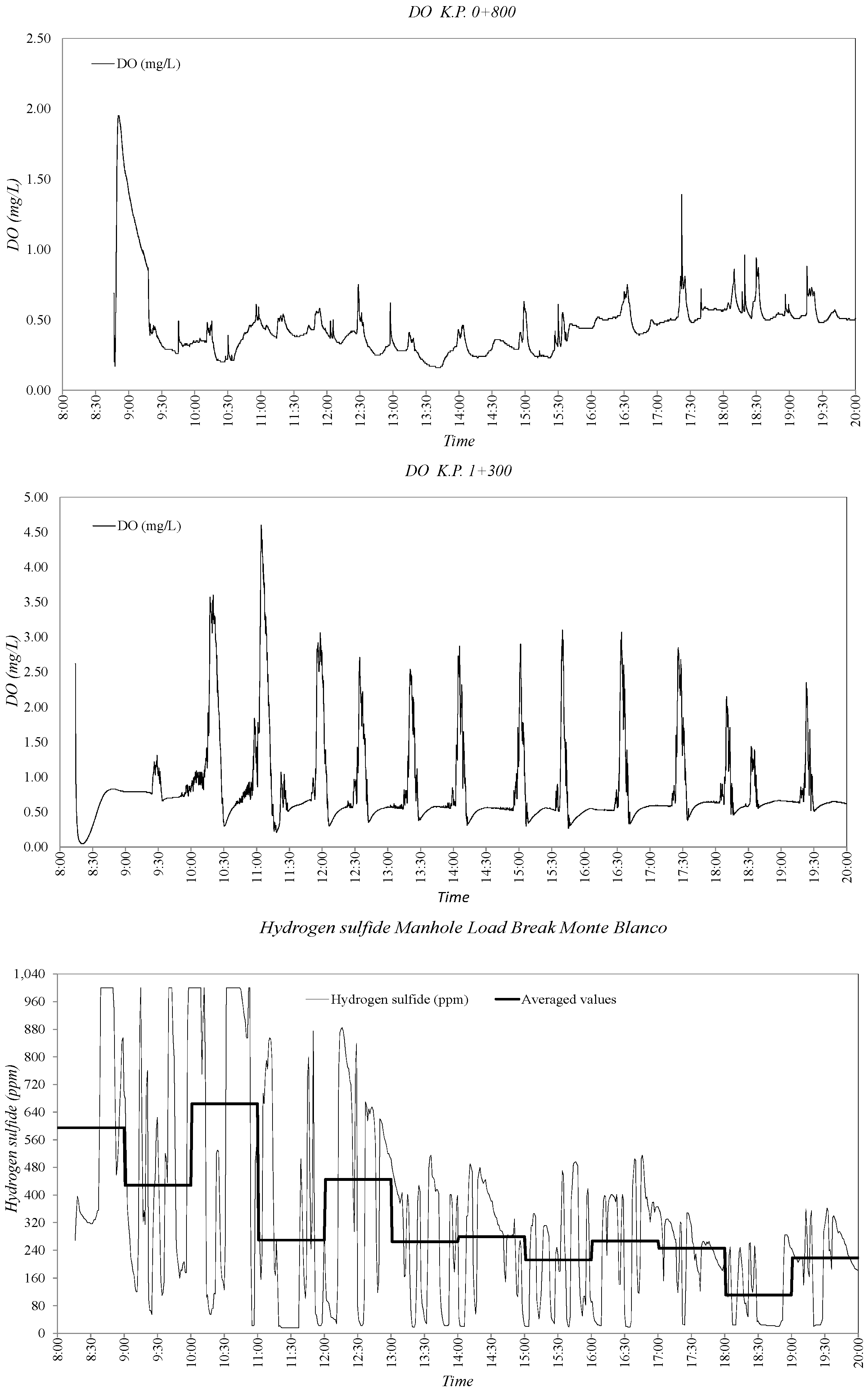
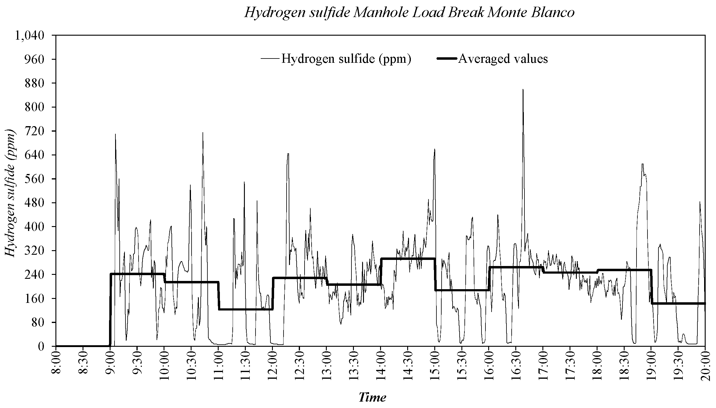
3.2. Sewer Pump Station Prototype Field Measuremments
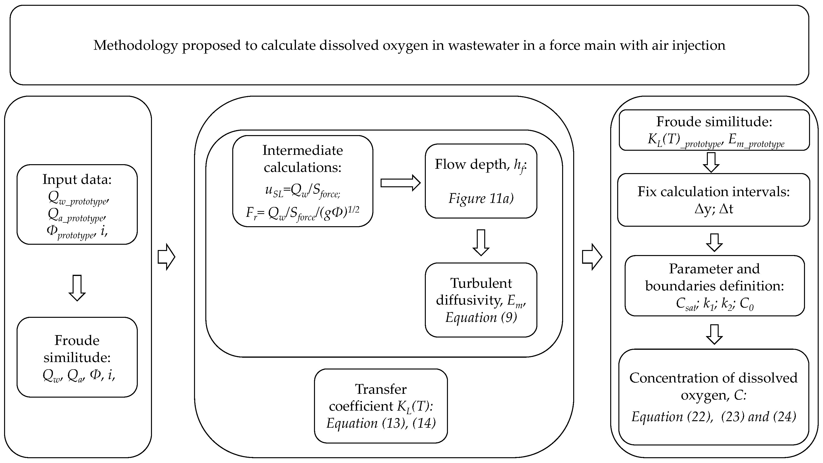
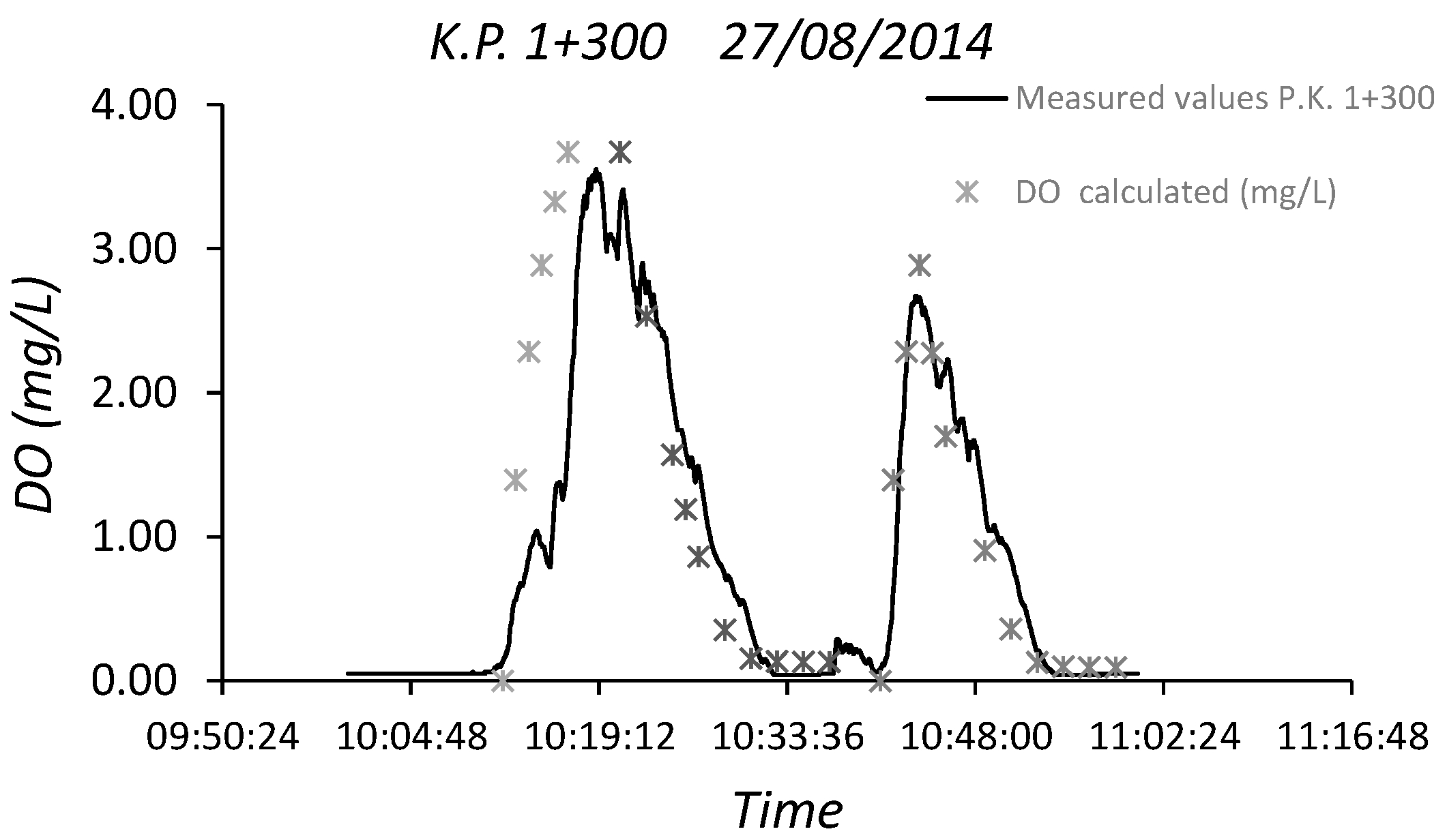
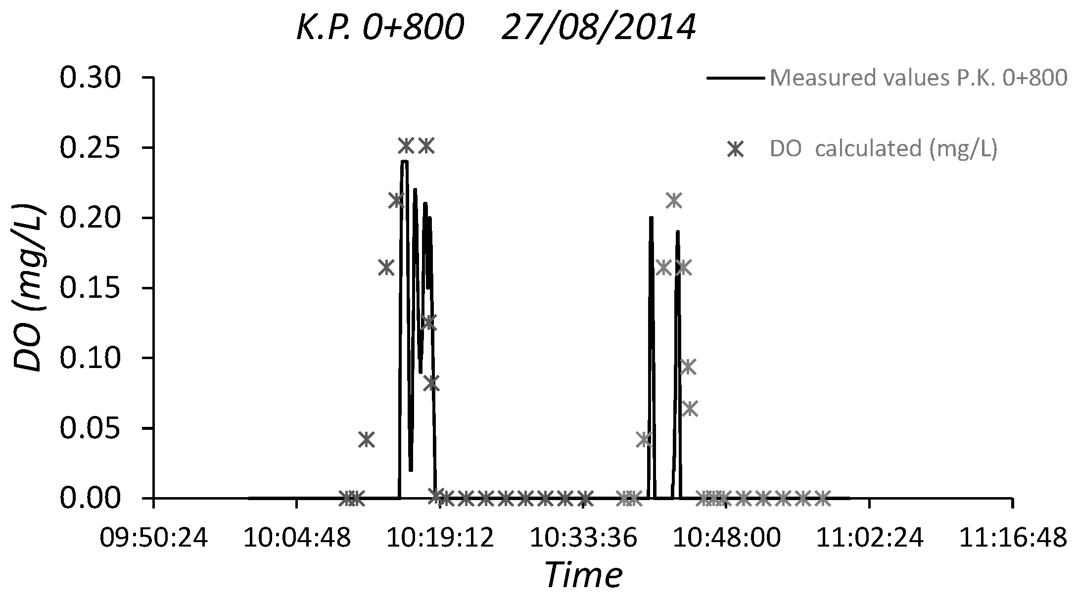
3.3. Dissolved Oxygen Prediction. Second Fick’s Law Application
4. Conclusions
Acknowledgments
Author Contributions
Conflicts of Interest
Appendix A

| Author Reference | Equation | Parameter Evaluated |
|---|---|---|
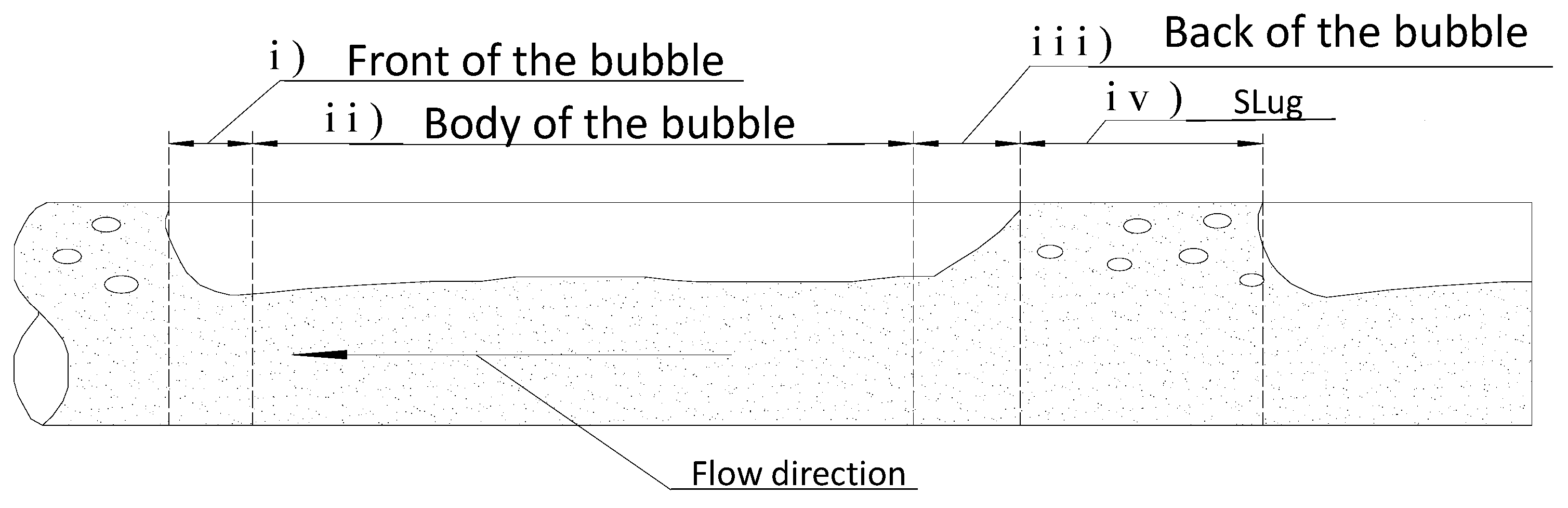
| Chu and Jirka (2003) [20] | ; ; . | KLw interphase mass transfer due to water flow (m/day); u*b shear (friction) velocity of water flow (m/s); hf flow depth in bubble zone (m); ff is the Darcy–Weisbach friction factor of water flow and pipe (-); uf is the velocity of the flow under the bubble (m/s) as seen in Figure 3; KLair interphase mass transfer due to airflow (m/day); u*a shear (friction) velocity of airflow (m/s); fi is the Darcy–Weisbach friction factor of air–water flow (-); uG mean velocity of the air inside the bubble (m/s); |
| Guilliver et al. (1990) [21] | ; ; ; ; | KLbubble due to mixture (m/day); DO2-H2O turbulent diffusivity in the water flow (m2/s); T = temperature (°K); ΨH2O = 2.26; MH2O = molecular weight of water =18 g/mol; µ = dynamic viscosity of water 0.890 (cP); VO2 = Molar volume of oxygen 25.6 cm3/g-mol; σ = surface tension of water 0.0728 kg/s2; bubble medium diameter; ε rate of turbulent kinetic energy dissipation per unit mass; and fraction of air in the slug and in the mixture zone respectively. |
| Measured at present work | lmixture of bubbles in the slug flow adjusted from observations (m); Ф inner diameter of pipe; Fr22 square Froude number Equation (1) adapted from [22]. |
References
- Hvitved-Jacobsen, T.; Vollertsen, J.; Nielsen, A.H. Sewer Processes: Microbial and Chemical Process Engineering of Sewer Networks; CRC Press: Boca Raton, FL, USA, 2013. [Google Scholar]
- Zhang, L.; De Schryver, P.; De Gusseme, B.; De Muynck, W.; Boon, N.; Verstraete, W. Chemical and biological technologies for hydrogen sulfide emission control in sewer systems: A review. Water Res. 2008, 42, 1–12. [Google Scholar] [CrossRef] [PubMed]
- Pomeroy, R. Generation and control of sulfide in filled pipes. Sew. Ind. Wastes 1959, 31, 1082–1095. [Google Scholar]
- Sewell, R.J. Controlling Sulfides in Sanitary Sewers Using Air and Oxygen; National Environmental Research Center: Cincinnati, OH, USA, 1975. [Google Scholar]
- Design Manual. Odor and Corrosion Control in Sanitary Sewerage Systems and Treatment Plants; Center for Environmental Research Information, US Environmental Protection Agency, Office of Research and Development: Washington, DC, USA, 1985. [Google Scholar]
- Tanaka, N.; Takenaka, K. Control of hydrogen sulfide and degradation of organic matter by air injection into a wastewater force main. Water Sci. Technol. 1995, 31, 273–282. [Google Scholar] [CrossRef]
- Kameda, Y.; Morita, T. Two-phase flow study using 300 mm diameter pipe. Jpn. J. Multiph. Flow 1990, 4, 219–249. [Google Scholar] [CrossRef]
- Kameda, Y.; Morita, T. Two-phase flow study using 200 mm diameter pipe. Jpn. J. Multiph. Flow 1993, 7, 250–261. [Google Scholar] [CrossRef]
- Ochi, T.; Kitagawa, M.; Tanaka, S. Controlling sulfide generation in force mains by air injection. Water Sci. Technol. 1998, 37, 87–95. [Google Scholar] [CrossRef]
- Tanaka, N.; Hvitved-Jacobsen, T.; Ochi, T.; Sato, N. Aerobic-Anaerobic Microbial Wastewater Transformations and Re-aeration in an Air-Injected Pressure Sewer. Water Environ. Res. 2000, 72, 665–674. [Google Scholar] [CrossRef]
- Taitel, Y.; Dvora, B. Two-phase slug flow. Adv. Heat Transf. 1990, 20, 83–132. [Google Scholar]
- Hanratty, T.J. Physics of Gas-Liquid Flows; Cambridge University Press: Cambridge, UK, 2013. [Google Scholar]
- Lauchlan, C.S.; Escarameia, M.; May, R.W.P.; Burrows, R.; Gahan, C. Air in Pipelines; Report SR; HR Wallingford: Wallingford, UK, 2005; p. 649. [Google Scholar]
- Barnea, D.; Shoham, O.; Taitel, Y.; Dukler, A.E. Flow pattern transition for gas-liquid flow in horizontal and inclined pipes. Comparison of experimental data with theory. Int. J. Multiph. Flow 1980, 6, 217–225. [Google Scholar] [CrossRef]
- Adrian, R.J.; Westerweel, J. Particle Image Velocimetry; Cambridge University Press: Cambridge, UK, 2010; ISBN 9780521440080. [Google Scholar]
- Thielicke, W.; Stamhuis, E.J. PIVlab—Time-Resolved Digital Particle Image Velocimetry Tool for MATLAB. Version 1.4. 2014. Available online: http://dx.doi.org/10.6084/m9.figshare.1092508 (accessed on 28 February 2017).
- Socolofsky, S.A.; Jirka, G.H. Environmental Fluid Mechanics 1: Mixing and Transport Processes in the Environment; Texas A and M University: College Station, TX, USA, 2005. [Google Scholar]
- Crank, J. Mathematics of Diffusion, 2nd ed.; Clarendon Press: Oxford, UK, 1975. [Google Scholar]
- Pai, T.Y.; Ouyang, C.F.; Liao, Y.C.; Leu, H.G. Qxygen transfer in gravity flow sewers. Water Sci. Technol. 2000, 42, 417–422. [Google Scholar]
- Chu, C.R.; Jirka, G.H. Wind and stream flow induced reaeration. J. Environ. Eng. 2003, 129, 1129–1136. [Google Scholar] [CrossRef]
- Gulliver, J.S.; Thene, J.R.; Rindels, A.J. Indexing gas transfer in self-aerated flows. J. Environ. Eng. 1990, 116, 503–523. [Google Scholar] [CrossRef]
- Hager, W.H. Energy Dissipators and Hydraulic Jump; Springer Science & Business Media: Berlin, Germany, 2013; Volume 8. [Google Scholar]


| Pipe Slope | 1% | 4% | Test |
|---|---|---|---|
| Water flow rate (m3/h) | 0; 1200 | 0; 1200 | A1–A8 |
| Airflow rate (m3/h) | 240 | 240 |
| Pipe Slope | 1% | 4% | Test |
|---|---|---|---|
| Water flow rate (m3/h) | 0, 3, 6, 9 | 0, 3, 6, 9 | B1–B16 |
| Airflow rate (m3/h) | 2.5, 5 | 2.5, 5 |
| Case | Em (m2/s) | KL(28) (m/s) | dp = hf − 0.3 (m) |
|---|---|---|---|
| K.P. 0 + 800; Qw = 1200 (m3/h); Qa = 240 (m3/h); i = 1% | 9.92 × 10⁻⁵ | 3.86 × 10⁻⁵ | 0.161 |
| K.P. 0 + 800; Qw = 0 (m3/h); Qa = 240 (m3/h); i = 1% | 6.32 × 10⁻⁵ | 2.21 × 10⁻⁶ | 0.127 |
| K.P. 1 + 300; Qw = 1200 (m3/h); Qa = 240 (m3/h); i = 4% | 1.31 × 10⁻⁴ | 6.41 × 10⁻⁵ | 0.057 |
| K.P. 1 + 300; Qw = 0 (m3/h); Qa = 240 (m3/h); i = 4% | 9.48 × 10⁻⁵ | 9.48 × 10⁻⁶ | 0.030 |
© 2017 by the authors. Licensee MDPI, Basel, Switzerland. This article is an open access article distributed under the terms and conditions of the Creative Commons Attribution (CC BY) license ( http://creativecommons.org/licenses/by/4.0/).
Share and Cite
García, J.T.; Vigueras-Rodriguez, A.; Castillo, L.G.; Carrillo, J.M. Evaluation of Sulfide Control by Air-Injection in Sewer Force Mains: Field and Laboratory Study. Sustainability 2017, 9, 402. https://doi.org/10.3390/su9030402
García JT, Vigueras-Rodriguez A, Castillo LG, Carrillo JM. Evaluation of Sulfide Control by Air-Injection in Sewer Force Mains: Field and Laboratory Study. Sustainability. 2017; 9(3):402. https://doi.org/10.3390/su9030402
Chicago/Turabian StyleGarcía, Juan T., Antonio Vigueras-Rodriguez, Luis G. Castillo, and José M. Carrillo. 2017. "Evaluation of Sulfide Control by Air-Injection in Sewer Force Mains: Field and Laboratory Study" Sustainability 9, no. 3: 402. https://doi.org/10.3390/su9030402