Thermal, Economic and Environmental Analysis of a Low-Cost House in Alice, South Africa

Abstract

Indoor and outdoor temperature variation results in heat transfer between the inner and outer space of a house, subsequently drifting the indoor temperature out of the thermal comfort zone. This leads to occupants spending a significant amount of their income on space heating and cooling to achieve thermal comfort. The aim of this study is to analyze the thermal, economic and environmental impact of a low-cost house. A low-cost house located in Golf Course, Alice was used as a case study. The outdoor and indoor weather conditions of the house were monitored for periods covering summer and winter seasons. To maintain indoor thermal comfort, 3412.57 kWh of heating and 3214.75 kWh cooling energy were required in winter and summer seasons, respectively. At a rate of 1 ZAR equal to 13.34 USD and 29.39 c/kWh, the energy consumption results in $1003.02 worth of heating energy in winter and $944.88 of cooling energy in summer. In both seasons, to supply the equivalent amount of thermal energy used in the house from a coal-fired power plant, 9.65 ton of CO₂, 81.71 kg of SO₂ and 39.50 kg of NO₂ gases will be emitted into the atmosphere. Promoting and enforcing energy efficient design in low-cost housing will not only bring about energy savings, but will also provide a year-round indoor thermal comfort.

1. Introduction

The rapid increase in energy consumption and greenhouse gas (GHG) emission in the building sector has led to the amendment of energy policies in many countries. Globally, the building sector consumes over 30% of total final energy, having increased by more than 35% since 1990. At the same time, it also accounts for 30% of CO₂ gas emission [1]. According to the International Energy Outlook 2016, global final energy consumption is expected to increase by an average of 1.8% per annum from 2012 to 2040 [2]. This is as a result of the transition of many emerging economies from traditional sources of energy to modern marketable sources such as electricity. The final energy consumption includes energy consumed through space heating and cooling, domestic activities, lighting and household utilization [3].

Despite the increasing energy consumption, energy poverty is still a major issue in some parts of the world. Energy poverty can be defined as a state whereby occupants or households lack access or resource to afford basic energy services. Over two billion people worldwide live without electricity and rely on solid fuels such as biomass fuels and coal for their energy needs [4]. According to the World Health Organization (WHO), indoor air pollution increases the risk of pneumonia among children and chronic respiratory diseases for adults. Annually, it is responsible for more than 1.5 million deaths. Two-thirds of which occur in Sub-Saharan Africa and Southeast Asia [5]. Across Europe and other parts of the world that experience winter season, cold housing as a result of energy poverty leads to morbidity conditions, such as circulatory, respiratory, and mental illness; flu; arthritis; rheumatism; etc. The Marmot Review indicates that more than one in four adolescents living in cold housing are at risk of multiple mental health problems compared to 1 in 20 adolescents who have always lived in warm houses. In addition, excessive winter deaths are attributed to the coldest quarter of housing and account for 21.5% of the death toll during the season. Nevertheless, countries with profound energy efficiency housing policies have experienced lower excess winter deaths [6]. The recommended indoor temperature by the WHO is 21 °C in the living room and 18 °C in the bedrooms for at least 9 h of the day [7]. Studies [8,9] show that there are three main drivers of energy poverty: low-income, high energy costs, and poor thermal efficiency and housing.

Locally, energy poverty in South Africa is primarily driven by accessibility to energy sources, low-income and poor thermal efficiency and housing. In a bid to eliminate the historical inequalities in South Africa, the government embarked on rapid construction of low-cost housing (LCH) and electrification of rural areas. Between 1994 and 2001, approximately 1.2 million LCH were constructed or under construction [10]. Despite the housing progress, housing demand still increases. Documented by the Financial Fiscal Commission, the housing backlog increased from 1.8 million in 1996 to an estimated 2.1 million in 2013 [11]. On the other hand, electrification of formal households (includes low-cost housing) increased from 36% in 1994 to 87% in 2012, i.e., 5.7 million formal households were electrified. These values indicate households connected to the national grid and renewable sources of energy [12]. However, the backlog of electrified household still remains about three million, with a target to electrify 97% by 2025 [13]. In addition, the government argued that the average poor household does not consume more than 50 kWh per month. Hence, this amount of electricity should be provided for free per month for their basic needs, such as water heating, ironing, lighting, powering of small television set and radio. In 2003, Free Basic Electricity (FBE) policy that provides free 50 kWh of electricity per month to poor household was lunched [14]. However, FBE is not reaching all its intended beneficiaries. As of 2015, only 77% of customers were documented as collecting their FBE tokens [15]. The energy poverty level in South Africa is estimated to be between 40% and 49% in 2015 [16]. FBE policy never took into consideration the thermal needs of the household, given the conditions of LCH.

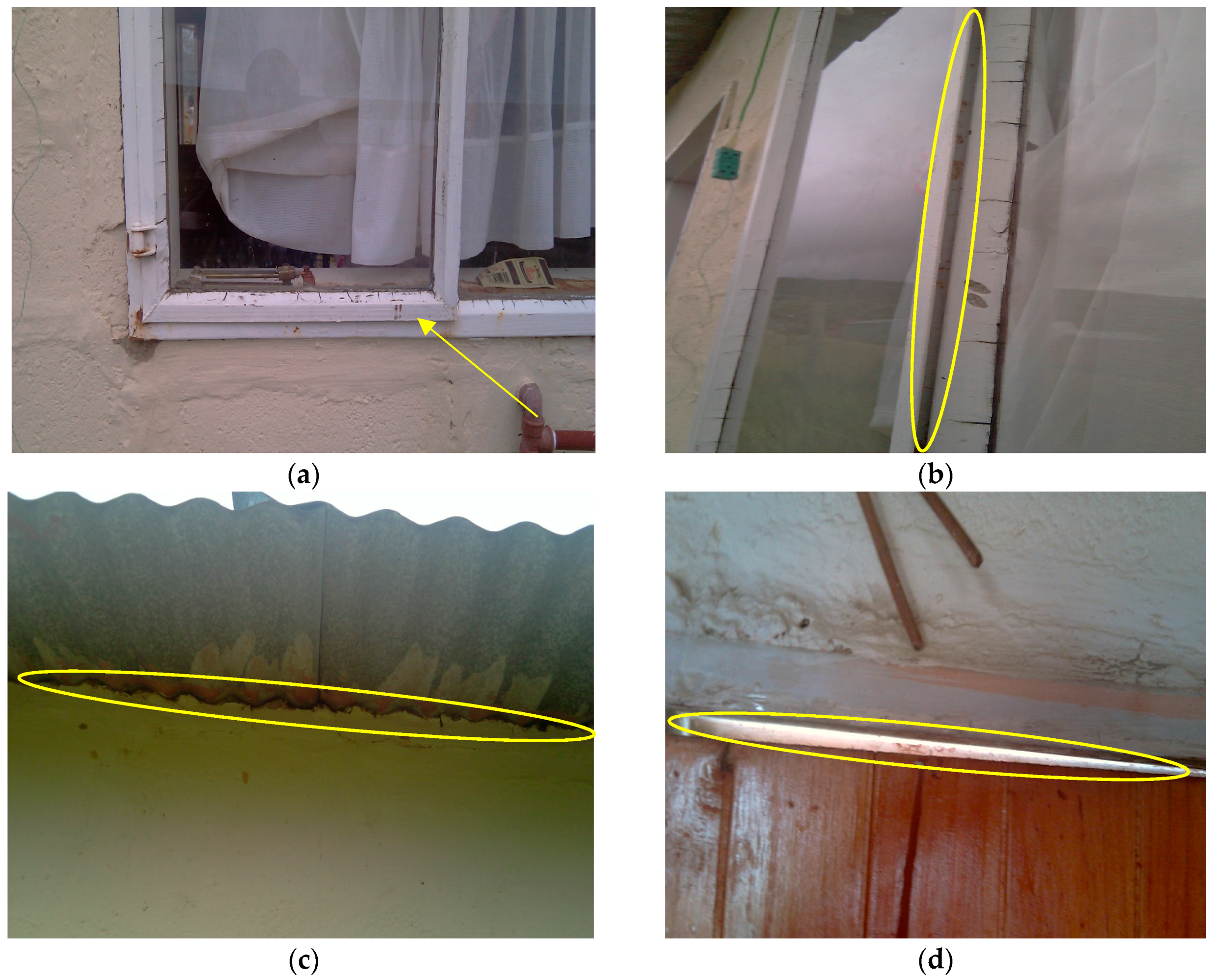
Over the years, LCH has been characterized by poor indoor air quality and harsh thermal conditions. Occupants finding their homes excessively hot in summer and extremely cold in winter [17,18]. This is as a result of poor building design and use of inferior building materials. Despite the high amount of solar radiation in South Africa, LCH lacks the capacity to utilize solar energy for space heating. Cracks, openings and poor thermal properties of the thermal envelope of LCH, results in uncontrolled heat exchange between indoor and the ambient environment. Thereby, creating a thermally discomfort environment indoors. Having exhausted the monthly FBE, households will spend a significant amount of their income on space heating to achieve indoor thermal comfort [19]. Alternatively, these households use coal, paraffin heaters or clothing to keep warm. This leads to poor indoor air quality, cold-related illness, CO₂ emission, etc. According to the Department of Minerals and Energy (DME) 2009, the residential sector represents the third largest energy demanding sector in South Africa, accounting for 20% of energy demand [12]. South Africa’s dependence on coal has resulted in the country being the leading CO₂ emitter in Africa, accounting for 40% of emissions. On a global scale, South Africa is the 13th largest CO₂ emitter according to Energy Information Administration (EIA) estimates [20].

Three-quarters of the total energy consumption in the building sector is residential, with great opportunity for energy improvement [21]. The building design and components of the thermal envelope are the main determining factor of energy consumption in residential buildings. Mari-Louise et al. investigated the influence of window size on the energy required to maintain the indoor temperature in between 23 °C and 26 °C. They used a dynamic building simulation tool (DEROB-LTH). They found that the size of the window is relevant for cooling energy in the summer but has no significant impact in the winter season. Mari-Louise et al. concluded that a smaller window was recommended on south elevation for minimum cooling energy needs [22]. The impact of opaque building envelope configuration on the heating and cooling energy needed in a cold climate was studied by Francesco et al. They argued that thermal transmittance and inertia are traditionally connected to two different energy demands. While thermal transmittance is crucial to reduce heating energy demand, thermal inertia has an impact on cooling energy demand. They discovered that the influence of thermal inertia on heating energy need is limited while periodic thermal transmittance has an impact on heating load [23]. In addition, Wang and Wong analyzed the impact of ventilation strategies and façade designs on indoor thermal environment of a residential building. They evaluated four ventilation strategies: nighttime only, daytime only, full-day and no ventilation. Parametric studies of façade designs on orientations, window to wall radio and shading device were performed using the building simulation tool (FLUENT). They found that full-day ventilation provides better indoor thermal comfort.

The above-cited research demonstrates the significance of building design and component of the thermal envelope on energy consumption. They also hinted at various energy efficiency measures for residential buildings via building design and thermal envelope. However, similar to most energy and sustainability research, economic and environmental impact of building energy consumption are not taken into consideration. In other words, these concepts (economic and environment) are not treated in detail. This study is focused on the thermal load, and economic and environmental impact of a low-cost house. Furthermore, the study portrays the social economic welfare of a LCH occupant as well as the environmental impact with respect the house thermal performance.

2. Thermal Comfort

The definition and control of indoor thermal comfort in buildings is difficult to establish due to the variation in the parameters involved [24]. Commonly, thermal comfort is defined as the condition of mind in which satisfaction is expressed with the thermal environment [25]. Thermal dissatisfaction is caused by the temperature of a body as a whole. This is as a result of unwanted heating or cooling of the body [26]. Sensible and latent heat losses from the skin are typically expressed in terms of environmental factors, skin temperature, and skin conditions (dry or wet). It also accounts for the thermal insulation and moisture permeability of clothing. The environmental variables can be summarized as air temperature, radiant temperature, relative air speed and humidity. The operative personal variables that influence thermal comfort are human activity and clothing [27].

The human perception of thermal comfort analysis conducted by Fanger in 1982 shows that the sensation of thermal comfort was most significantly determined by narrow ranges of skin temperature and sweat evaporation rate, depending on activity level. More active people were comfortable at low skin temperatures and higher evaporation rates. By combining this information with the ASHRAE thermal sensation scale, shown in

Table 1. ASHRAE thermal sensation used by Fanger.

PMV	Sensation
−3	Cold
−2	Cool
−1	Slightly cool
0	Neutral
+1	Slightly warm
+2	Warm
+3	Hot

Source: Principles of Thermal Comfort [26].

, Fanger developed a comfort index called PMV [26,28].

PMV is an index that predicts the mean value of the votes of a large group of persons on a seven-point thermal sensation scale [29]. The PMV index can be determined when the activity (metabolic rate) and the clothing (thermal resistance) are estimated, and the following environmental parameters are measured: air temperature, mean radiant temperature, relative air velocity and partial water vapor pressure. The PMV is given by the equation [26];

$$\begin{array}{l}PMV=(0.303e^{-0.036M}+0.028)\{(M-W)-3.05\times {10}^{-3}[5733-6.99(M-W)-0.42[(M-w)-5815]\\ -1.7\times {10}^{-5}(5867-P_a)-0.0014M(34-t_a)-3.96\times {10}^{-8}{f}_{cl}[{(t_r+273)}^4]-f_{cl}{h}_c(t_{cl}-t_a)\}\end{array}$$

(1)

where

• M = Metabolic rate (W/m²);
• w = External work (W/m²);
• P_a = Partial water pressure (Pa);
• t_a = Air temperature;
• f_cl = Ratio of clothed surface to nude surface area;
• t_r = Mean radiant temperature; and
• h_c = Convective heat transfer coefficient (W/m^2.K).

PPD is a predicted value calculated from PMV. It predicts the percentage of people dissatisfied with the thermal conditions of their surroundings [30], people who felt more than slightly warm or slightly cold (i.e., the percentage of the people who inclined to complain about the environment). Using the thermal sensation scale in Table 1, Fanger postulated: people who respond ±2 and ±3 are uncomfortable, while those who respond ±1 and 0 are comfortable. The relationship between PPD and PMV is given by Equation (2);

$$PPD=100-95e^{-\left(0.03353PM{V}^4+0.2179PM{V}^2\right)}$$

(2)

Owing to individual differences, it is impossible to specify a thermal environment that will satisfy everybody: if the PMV is zero, 5% of people are dissatisfied. It is possible, however, to specify environment known to be acceptable by a certain percentage of the occupants. The ISO standard 7730, for example, recommends that the PPD should be lower than 10%, i.e., PMV within the range of ±0.5 [31].

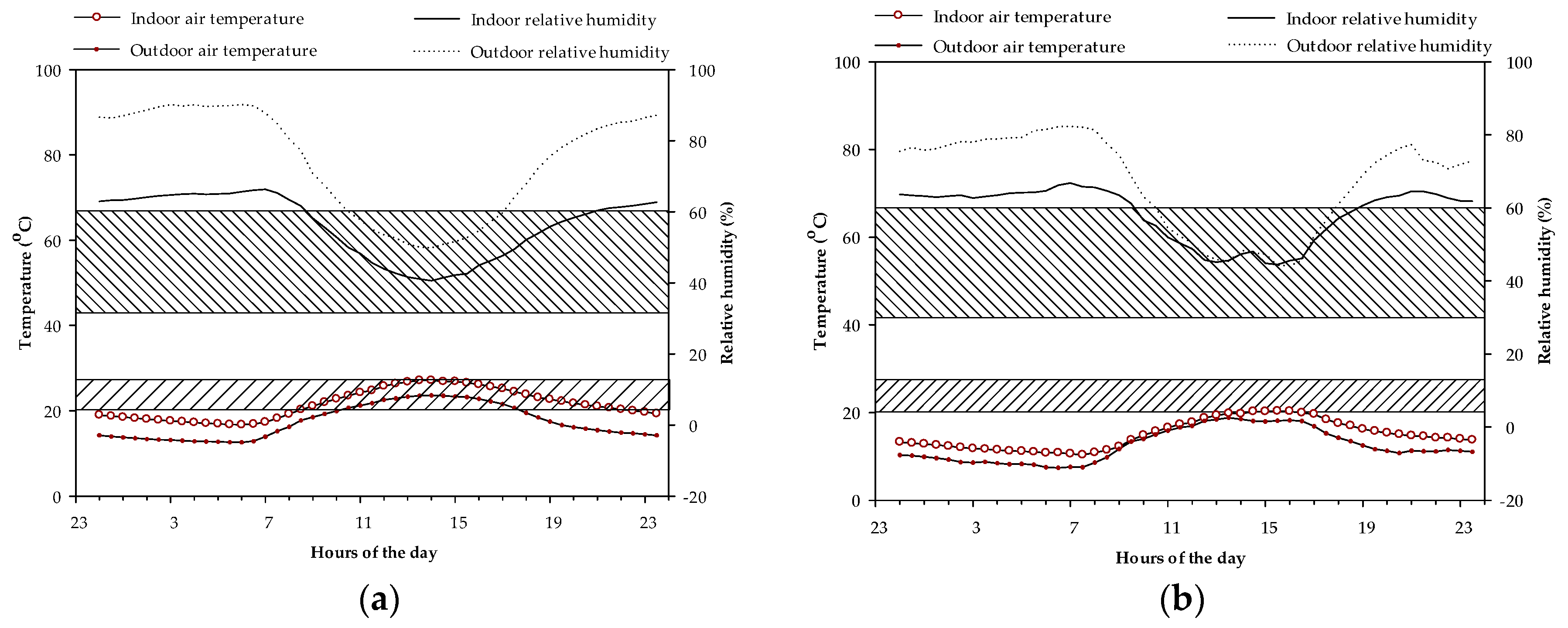
Another approach for analyzing thermal comfort was done by the American Society of Heating, Refrigeration and Air-Conditioning Engineers (ASHRAE) standard 55 and ISO standard 7730. In this method, thermal comfort depends on indoor temperature and relative humidity. A fix and uniform temperature range and a lower and upper humidity level were set for winter and summer seasons. Low humidity (dew point less than 0 °C) results in dry skin and mucous surfaces leading to comfort complaints such as dry nose, throat, eyes, and skin. High humidity also results in discomfort due to increased moisture, friction between skin and clothing, increased skin moisture, etc. To prevent thermal discomfort, the recommended lower and upper relative humidity levels should not exceed 30% and 60%, respectively [25,32], whilst the indoor temperature is kept at 20 °C to 23 °C in the winter and 24 °C to 26 °C in the summer season. The South African National Standards (SANS) 204 recommend 20 °C to 24 °C indoor temperature in both seasons and 30% to 60% relative humidity [33].

3. Thermal Load Estimation

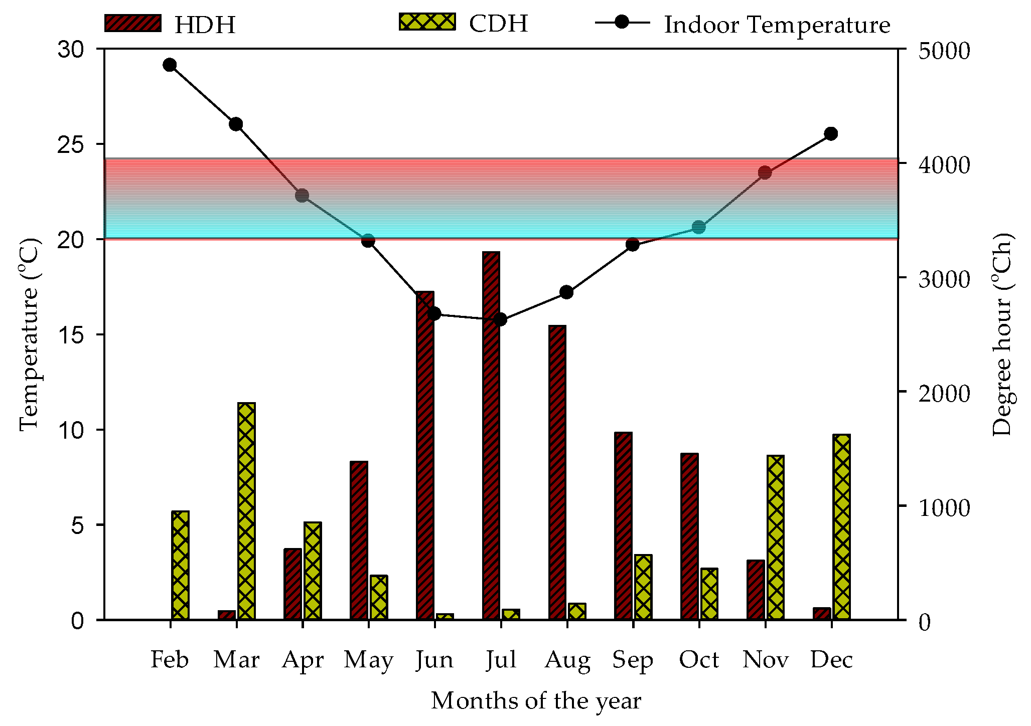
Reliable and sufficient results can be achieved when using steady-state heat transfer analysis to estimate building thermal load [34]. However, various methods can be used to estimate building thermal load: radiant time series, thermal network, heat balance, degree hours, etc. Degree-hours is an easy to use, and well-established tool for energy consumption analysis in buildings [35]. Degree-hours is the sum of the difference between hourly average temperatures and a reference temperature. The numbers of heating (HDH) and cooling (CDH) degree-hours are given as:

$$HDH={\displaystyle \sum _m{(T_b-T_{av})}^{+}}$$

(3)

$$CDH={\displaystyle \sum _m{(T_{av}-T_b)}^{+}}$$

(4)

$T_{av}$ and $T_b$ represent the average hourly and reference based temperature, respectively. The positive sign implies that only positive values are considered. In addition, m indicates monthly degree-hours. That is, the sum of daily degree-hours in a given month. It could also be extended or reduced to yearly or daily degree-hours, respectively. The monthly or seasonal thermal load can be determined by

$$q_{h,c}=(U)D{H}_{h,c}$$

(5)

where $q_{h,c}$ is cooling or heating load (kWh/m²); $D{H}_{h,c}$ is the total heating or cooling degree-hours (°C·h); and $U$ is the overall heat transfer coefficient (W/m²·K) of the opaque components of the thermal envelope. It is the sum of the thermal transmittance (U-value) of all opaque components of the thermal envelope that experience temperature change from inside to outside of the building. According to the First law of thermodynamics, the net change in the total energy of a system is the total energy entering and leaving the system. Therefore, to maintain a stable thermal condition indoors, the equivalent amount of heat gain or loss has to be removed (cooling) or supplied (heating), respectively. Hence, the heating or cooling energy required to maintain a stable indoor thermal condition is given by:

$$Q_{h,c}=\frac{UA}{{\eta }_{h,c}}D{H}_{h,c}$$

(6)

where $Q_{h,c}$ is the monthly heating or cooling energy (kWh), A is the total floor surface area of the house and ${\eta }_{h,c}$ is the efficiency of the heating or cooling system. The monthly cost of energy consumed for heating or cooling can be determined from Equation (7):

$$R_{h,c}=Q_{h,c}{C}_E$$

(7)

$C_E$ represents energy charge per unit (c/kWh). In South Africa, energy charges vary with tariff structure. Tariff structures are designed based on customer’s consumption, and they include urban (maximum load > 1 MW), residential (maximum load ≤ 0.1 MW) and rural (maximum load of 0.025 MW) [36].

Greenhouse Gas Emission

Coal-fired power stations are the main source of electricity in South Africa. This implies that domestic energy consumption contributes to greenhouse gas emission of the country. The greenhouse gas emission and other environmental impact due to the total energy generated and supplied per annum (financial year) are determined by the national power authority (Eskom). This is done using the IPCC 2006 guidelines for the UNFCCC methodology [37,38]:

$${\alpha }_X=E{F}_X\left[\frac{{\displaystyle \sum _y{Q}_{h,c}}}{1000}\right]$$

(8)

where $Q_{h,c}$ is cumulative monthly heating or cooling energy (MWh), ${\alpha }_x$, is the emission of x gas per annum and $E{F}_x$ is emission coefficient of x gas, which could be CO₂, CH₄, NO_x, SO_x, etc. Emission factors are usually determined per annum and they vary from one country to another as they are influenced by the primary means of energy production.

4. Description of the House and Its Location

The house used as case study is located in the Golf Course settlement Alice under the Raymond Mhlaba Municipality, Eastern Cape. Golf Course is geographically located at 32°S latitude and 26°E longitude, at an altitude of 493 m. According to the Köppen–Geiger climate classification, Alice has a BSh Arid, Steppe, Hot arid climate. Such climate is characterized by annual precipitation greater than 5 P_th. The annual temperature is greater than or equal to +18 °C [39]. 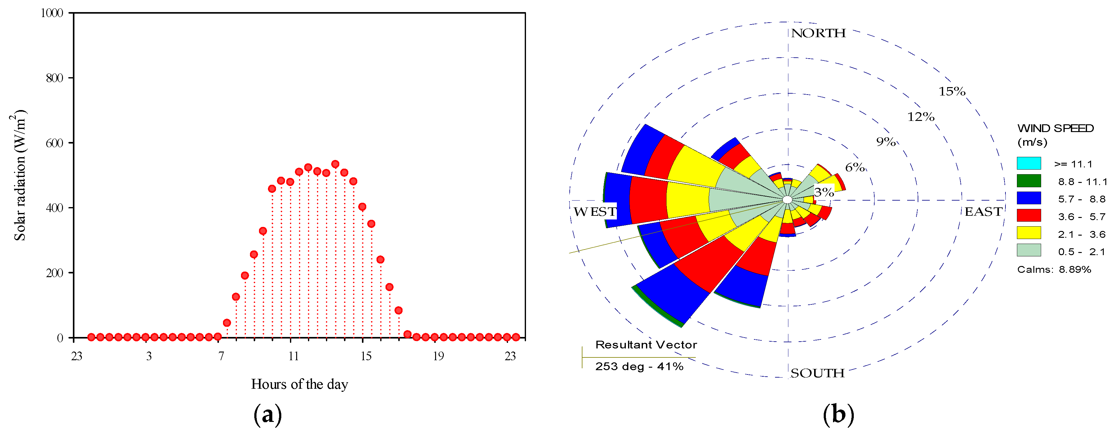Locally, Alice is in the temperate interior (Zone 2) climate of South Africa [40]. The climatic conditions are characterized by a hot summer and mild (no snow) winter, with an average dry bulb temperature of 29 °C and 15 °C, respectively. Rainfall usually occurs in the summer season while winter season is characterized by dry, dusty and windy conditions. 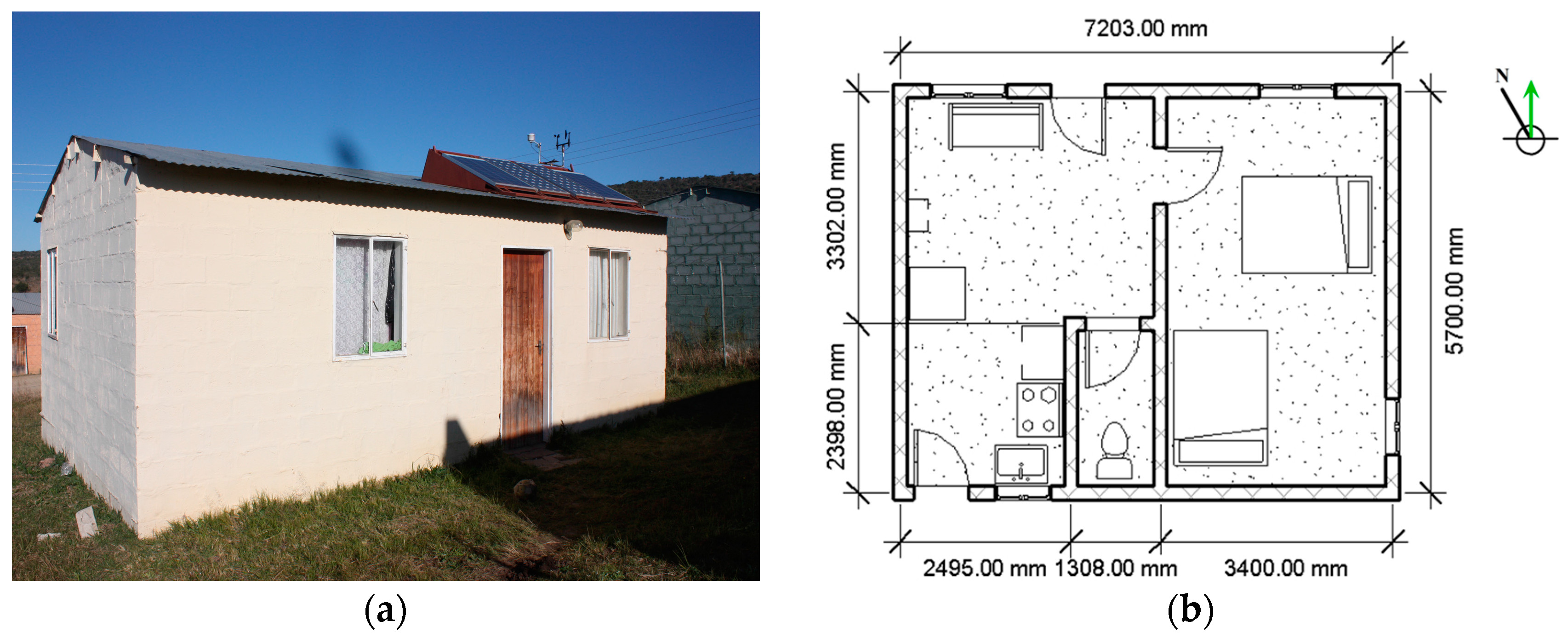The east wind is predominant in summer while the winter is dominated by the west wind [41]. An average wind speed of 2.5 m/s is experienced in Golf Course throughout the year. Similar to most LCH settlements in the country, Golf Course is a rural settlement primarily occupied by senior citizens, children and low-income earners. The LCH used in this study and its floor plan are shown in Figure 1a,b.

The passive solar features of the house such as the orientation (16° east of north) and large North facing windows were the major reasons the house was selected. The house comprises of a bedroom, bathroom, open plan living room and kitchen. The total floor dimension is 7.20 m × 5.70 m, approximately 41 m² floor area. The height of the house at the mid-wall and perimeter walls is 2.89 m and 2.44 m, respectively. The roof is made of galvanized, corrugated iron sheets with no ceiling or any form of roof insulation. The walls are made of M6 (0.39 × 0.19 × 0.14 m) hollow concrete blocks, with no plaster or insulation. Thus, the thickness of the walls assumed the width (0.14 m) of the blocks. More than 97% of the houses in this settlement share the same design.

5. Methodology

To monitor the weather parameters of the house, a series of meteorological sensors were installed. These include type K thermocouple, HMP50 temperature–humidity probes, Li-Cor pyranometer and 03001 wind sentry anemometer and vane.

Type K thermocouple is made of two dissimilar metals joined near the measurement point. It consists of a measurement and reference junction. The reference junction is created where the two metals connect to the measuring point. Type K thermocouple produces a micro-voltage signal which is related to the temperature difference between the measurement and reference junctions. With an error of 2.20 °C, type K thermocouple has a temperature measurement range of −200 °C to 1250 °C [42]. The HMP50 temperature and relative humidity probe contains a platinum resistance temperature detector (PRT) and a capacitive relative humidity sensor. It has a temperature and relative humidity range of −26 °C to 60 °C and 0% to 98%, respectively. It has an accuracy of ±3% with a response time of 15 s. To ensure precise measurement of the ambient temperature and humidity, the HMP50 was housed in a solar radiation shield in outdoor measurement [43]. Li-Cor pyranometer is used to measure the global solar radiation, i.e., the sum of direct and diffuse radiation. The Li-Cor pyranometer employs a silicon photovoltaic sensor which is mounted in a cosine-corrected head. The current measured by the detector is converted to a voltage signal by a shunt resistor in the sensor cable [44]. The wind sentry anemometer and vane measure the horizontal wind speed and wind direction. The anemometer has a range of 0 to 50 m/s. The cup wheel rotation produces an AC sine wave voltage with frequency directly proportional to wind speed. This AC signal is induced in a stationary coil by a two-pole ring magnet mounted on the cup wheel shaft. One complete sine wave cycle is produced for each cup wheel revolution. On the other hand, Wind vane position is transmitted by a 10 K ohm precision conductive plastic potentiometer, which requires a regulated excitation voltage. With a constant excitation voltage applied to the potentiometer, the output signal is an analogue voltage directly proportional to azimuth angle [45].

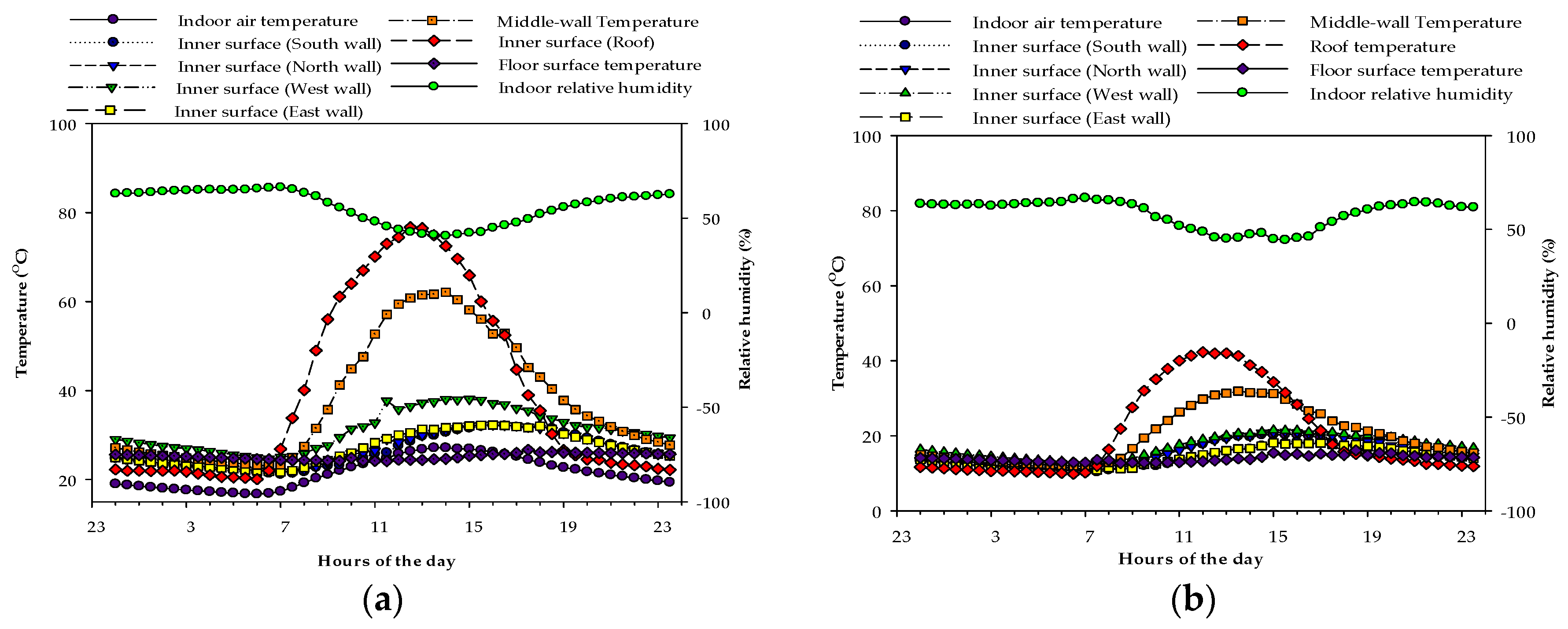
A total of 13 thermocouples were used to measure the indoor air, roof, floor, walls inner and outer surface temperatures. The indoor air thermocouple was placed at a height of 1.80 m to have good indoor air temperature variation patterns that are not influenced by the roof temperature and stack warm air. The same height was adopted for the thermocouples measuring the walls surface temperature. They were mounted such that their sentry terminals are in a direct contact with the walls’ surface. One thermocouple on each side of the wall was used to measure the inner and outer surface temperature of the north, east, west and south walls. Indoor relative humidity was measured by a temperature–humidity probe placed at same height as the indoor air thermocouple. Conversely, outdoor air temperature and relative humidity were measured via a solar radiation shielded temperature–humidity probe. The Campbell Scientific 41303-5A 6-plate radiation shield was used [43]. It is designed to allow ventilation, while at the same time preventing solar radiation from affecting the probe (sensor). The wind sentry anemometer/vane and pyranometer were used to measure wind speed/direction and global solar radiation, respectively. The outdoor metrological sensors were installed at a height of 0.44 m above the roof of the house. The entire sensors were then connected to a Campbell Scientific CR1000 datalogger supported by an AM 16/32 relay multiplexer, powered by a 20 V battery charged by a 20 W solar panel.

6. Results and Discussion

The house was monitored for a period covering all seasons in South Africa, which are autumn, winter, spring and summer. Climatic or energy performance analysis are usually done based on the assumption that June to August are winter seasons while September to May represent summer seasons [46,47]. During the period of this study, the household was made up of a middle-aged woman, her teenage daughter and a toddler. It was observed that the householder was unemployed and spent most of her time indoors while her daughter goes to school. During the weekends, the house is occupied by the occupants, friends and other visiting family relatives. No mechanical heating or cooling system was used by the occupants. They often rely on natural ventilation for cooling in hot sunny days and use thick clothes or paraffin heater to stay warm in cold days. The results of the measured weather parameters, and calculated economic and environmental impact due to the energy required to maintain indoor thermal comfort are presented and discussed in this section.

6.1. Thermal Behaviour of the House

According to the ASHRAE standard 55 and ISO standard 7730, air temperature and humidity plays a major role in the indoor thermal comfort [25,32]. Heat exchange between the inner and outer space of the house, through the components of thermal envelope, creates indoor temperature and humidity variation. The indoor temperature and relative humidity response to the outdoor temperature and relative humidity for the monitoring period is shown in Figure 2. It was observed that the indoor temperature closely followed the outdoor temperature variation, but attained higher peak temperatures with an average time lag of 1 h. The maximum indoor and outdoor temperatures of 32.99 °C and 30.59 °C, respectively, were also observed in the month of February. The minimum outdoor temperature of 4.87 °C was observed in July, while the corresponding indoor temperature was 9.90 °C. The mean indoor and outdoor temperature difference for the monitoring period was 3.40 °C/day.

On the other hand, the outdoor temperature has an inverse influence on both the indoor and outdoor relative humidity. Outdoor and indoor relative humidity varied from 33% to 94% and 31% to 73%, respectively. The mean indoor relative humidity was 57% while the outdoor relative humidity was 72% during the entire monitoring period.

Seasonal thermal behavior of the house was analyzed using a typical summer and winter day profile. Figure 3a,b shows the indoor temperature and relative humidity distribution on a typical summer and winter day. In both figures, the upper and lower shaded bars represent the SANS recommended indoor relative humidity and temperature limit, respectively, for indoor thermal comfort. In Figure 3a, the indoor temperature was found to be within the comfort zone for approximately 63% of the day. During this period, the average indoor temperature was 21 °C with a daily swing (maximum and minimum temperature difference) of 10 °C. The indoor relative humidity was also observed to be within the comfort zone for a significant period of the day. However, during the early hours of the day, the indoor temperature was below the thermal comfort zone by an average of 3 °C, while the relative humidity was above the comfort zone by an average of 4%.

The house exhibits a relatively poor thermal behavior in the winter season. As seen in Figure 3b, the indoor temperature was in the comfort zone for only 2 h of the day. It closely followed the outdoor temperature, with 1.5 h delay and mean temperature difference of 2 °C. At 07:30, the indoor temperature was at its minimum of 10.35 °C while the indoor relative humidity was at its peak with 67%. A mean difference of 9% was observed between the outdoor and indoor relative humidity. The indoor relative humidity was 4% above the comfort zone while the indoor temperature was 6 °C below.

Furthermore, the thermal condition of the house with regard to PMV was analyzed via the Centre for the Built Environment (CBE) online thermal comfort tool kit [48]. The average inner surface temperatures of the thermal envelope components were used as the mean radiant temperature. The indoor air speed was limited to 0.1 m/s due to no occupant control. Summer and winter conditions were distinguished by typical indoor clothing level. Typical summer and winter indoor clothing level of 0.5 clo and 1.0 clo, respectively, were used. The thermal response of the occupants while performing selected activities are summarized in

Table 2. Predicted thermal response of occupants.

Activities	Metabolism (w/m2)	Summer			Winter
		PMV	PPD (%)	Sensation	PMV	PPD (%)	Sensation
Sleeping	40	−2.08	80	Cool	−4.80	100	Very cold
Seated, quiet	45	−0.14	5	Neutral	−2.03	78	Cool
Standing, relaxed	70	0.30	7	Neutral	−1.27	39	Slightly cool
Cooking	104	1.02	27	Slightly warm	−0.11	5	Neutral
House cleaning	157	1.86	70	Warm	0.83	20	Slightly warm

.

The PMV also shows that a more thermally favorable condition was achieved in summer compared to winter. On a typical summer condition with an average indoor air temperature of 21 °C, 80% of occupants while sleeping will feel cool (uncomfortable). In the same thermal conditions, 7% of occupants standing relaxed will feel thermally comfortable while the remaining 93% might be thermally uncomfortable. On the other hand, at an average indoor air temperature of 14 °C on a typical winter condition, 100% of occupants while sleeping will feel very cold. As indicated in Table 1, the sensation scale ranges from −3 (cold response) through 0 (neutral) to +3 (hot response). Hence, −4.80, which is above the scale, is considered to be a very cold response. Nevertheless, 5% and 20% of occupants cooking and housing cleaning, respectively, willing feel thermally comfortable.

6.1.1. Influence of Ambient Weather Conditions

Solar radiation and wind are the weather factors that influence the thermal conditions of a building the most. The infrared component of solar radiation generates heat in the inner space of a building, whereas wind is often utilized for cooling. Hence, the summer daily average solar radiation distribution and wind profile of the house are shown in Figure 4a,b. An average solar radiation of 606.06 W/m² was experienced at the house location, as seen in Figure 5a. A peak solar radiation of 983.17 W/m² was observed at 12:30. With a 2 h delay, this corresponds with the period the indoor and outdoor air (Figure 3a) attained their peak temperature. At the same time, the indoor and outdoor relative humidity was at their minimum. This indicates an inverse relationship between solar radiation and relative humidity and direct relationship with temperature. Therefore, an increase in solar radiation will increase the indoor temperature of the house, while, at same time, decreasing the indoor relative humidity.

The wind rose profile of the house was generated using measured hourly summer wind speed and direction data. The prevailing wind is indicated by the resultant vector which was determine by the frequency count of the mean wind direction. From Figure 3b, the Southeast prevailing wind was experienced in the summer season, blowing from a mean direction of 154°. The average wind speed during this period was 2.6 m/s and 8.48% calm. Based on the orientation of the house and the location of the windows (Figure 1a,b), the occupants will experience passive cooling through cross ventilation. This will however depend on the operation of the windows, as it requires a free flow of air from the south to north facing windows [49]. It was noticed that the occupants often leave the kitchen and living room doors open during warm sunny days. Although the windows were shut, warm air at the north elevation force the rush of cool air through the inner space of the house, thereby cooling the indoor temperature and maintaining thermal comfort as seen in Figure 3a.

Unlike the summer season, a fairly harsh indoor environment was experienced in the winter season, as seen in Figure 3b. This can be attributed to the ambient weather conditions during the season. Figure 5a,b, shows the daily average winter solar radiation distribution and wind profile, respectively. Considering periods between 07:30 and 17:30 in Figure 5a, the average solar radiation during these periods was 346.17 W/m² and a maximum of 621.72 W/m². This is 38% less than the peak solar radiation experienced in the summer season.

The Southwest prevailing wind, blowing at an average speed of 2.84 m/s was observed in the winter season. Although it was noticed that the occupants always shut their doors and windows during the winter period, openings and cracks on the thermal envelope appeared to be a major issue in the house. Figure 6a–d shows some of the areas with unintentional openings on the thermal envelope of the house.

These openings increased the infiltration rate of the house in the winter season. Wind forces cold and humid air through these openings into the inner space of the house, which reduces the indoor air temperature and increases the relative humidity. The occupants however tried to prevent heat loss through these openings by using rags and other material to seal the holes. Their actions made no significant difference given the thermal behavior of the house in the winter season.

6.1.2. Influence of Thermal Envelope

The thermal envelope is a major factor that determines the thermal behavior of a building. The components of thermal envelope as stated earlier comprise the roof, floor, walls and windows. Wind however flows through the openings on the thermal envelope and directly influenced the indoor weather condition. In addition, solar radiation penetrates the fenestration into the inner space of a building. This is referred to as solar heat gain through transparent components. Opaque component heat gain and conductive heat gain indirectly influence the indoor weather conditions. The analysis in this section is based on steady-state conductive heat transfer through the opaque components of thermal envelope. The indoor temperature and relative humidity response to the opaque component of the thermal envelope is shown in Figure 7a,b.

In both seasons, the roof exhibited the highest temperature with an average of 39.75 °C in summer and 20.57 °C in winter. Its maximum temperature was 76.70 °C and 42.29 °C in summer and winter seasons, respectively. The middle-wall temperature, i.e., the wall demarcating the bedroom and the living room, was observed to closely follow the roof temperature with an average temperature of 37.85 °C in summer and 19.79 °C in winter. Despite the relatively high temperature of both components, the indoor temperature was observed to closely follow the temperature of the perimeter walls. The roof of the house is made of galvanized iron sheet of 0.3 mm thick. Galvanized iron sheets are good thermal conductor but have a very low thermal storage capacity. Therefore, the roof rapidly loses heat as it is gained, thereby making no significant impact on the indoor temperature. In addition, during the day, warm air indoor rises to the roof due to convectional current, thereby increasing the air temperature closer to the roof and the roof surface temperature. This creates an almost stagnant vertical temperature gradient, trapping the heat to the roof. The perimeter walls make up 40% of the entire house surface area, not including the windows and doors, while the roof and floor form 30% each of the total surface area of the house. As a result, the perimeter walls contribute more heat to the inner space of the house and control the indoor temperature variation.

However, each of the perimeter walls has its own degree of contribution, as seen in Figure 7a,b. The orientation of the walls with respect to the position of the Sun influences the individual impact of the walls. In summer, the average inner surface temperature of the north, east, south and west facing walls were 26.76 °C, 26.93 °C, 26.36 °C and 31.08 °C, respectively, while the indoor temperature was 21.52 °C. An average temperature difference of 6.26 °C was observed between the perimeter walls and indoor air. The indoor temperature daily swing was 10.42 °C. On the other hand, the perimeter walls daily temperature swing was 10.63 °C, 10.51 °C, 10.95 °C and 13.42 °C for the north, east, south, and west walls, respectively. With a 0.09 °C daily temperature swing difference between the east wall and indoor air, it can be said that the east wall has the most influence on the indoor temperature. In addition, in winter season, the indoor temperature was dominated by the north wall, with a daily temperature swing of 0.17 °C. The average indoor temperature during the season was 14.93 °C. An average surface temperature of 15.75 °C, 14.32 °C, 14.17 °C and 17.18 °C was observed for the north, east, south and west walls, respectively.

To quantify the thermal contribution of each of the perimeter walls, Fourier steady state heat transfer equation was used, i.e., $q=-kA\frac{\Delta T}{\Delta l}$. The thermal conductivity, $k$, of hollow concrete block was assumed to be 0.51 W/m^.°C [50]. The thickness, $\Delta l$, of the walls as stated in Section 4 is 0.14 m. $\Delta T$ represents the difference between the outer and inner surface temperature of the walls. Hence, a negative $q$ indicates the rate of heat loss and positive $q$ represents heat generated. Figure 8a,b shows the perimeter walls rate of heat transfer in summer and winter seasons, respectively.

In both seasons, the west wall has the highest rate of heat gain and loss. This is because of the relatively high temperature (Figure 7) of the wall in both seasons. Apart from the considerable amount of solar radiation received during the day, the west facing wall is a whole-block wall. In other words, it has no windows or doors (Figure 1). As a result, its temperature gradient tends to change steadily at the slightest variation of the ambient temperature. The west wall exhibits a typical behavior of a thermal mass wall. Due to its location in the house, the wall is more of a problem than a passive source of energy. During the day, the wall absorbs and stores heat; as the ambient temperature drops after sunset, the heat is released to the inner and outer space of the house. On hot sunny day, this could result in overheating of the house. Likewise, it also serves as a channel of heat loss for internal heat generated in a typical cold winter day. On the other hand, the south facing wall is the least active as compared to the other walls. Despite its large surface area (14.58 m²), the wall received little to no direct solar radiation during the day in both seasons. This led to a small temperature gradient and high concentration of cold and moist air on both sides of the wall. For this reason, and as seen in Figure 8, the south wall of the house is one of the major sources of heat loss. In Figure 8, the area under the curves gives the daily average heat loss or generated by each of the walls. The amount of heat lost or generated by each of the perimeter wall in summer and winter seasons is summarized in

Table 3. Perimeter walls average heat transfer.

Perimeter Walls	Surface Area (m2)	Summer Average Daily Energy (kJ/h)		Winter Average Daily Energy (kJ/h)
		Loss	Generate	Loss	Generate
North	13.82	1.28	0.27	0.86	0.65
East	13.14	1.90	0.22	0.93	0.28
South	14.58	2.16	0.01	1.15	0.06
West	13.90	4.49	1.22	2.59	1.27

.

6.2. Heating and Cooling Load

In previous sections, the relatively poor thermal behavior of the house during the winter season was observed with decent indoor weather conditions in summer. It was seen that the ambient weather conditions influence the indoor weather conditions. This occurs through intentional (windows) or unintentional (cracks) openings on the thermal envelope, as well as heat transfer across the opaque components of the thermal envelope. To estimate the thermal load of the house due to its thermal behavior, the heating and cooling degree-hours was first determine using Equations (3) and (4). Traditionally, degree-hours is simply the sum of the difference between the average outdoor air temperature and reference temperature. However, the average indoor air temperature was used in place of the outdoor air temperature since it was measured and known. The reference based temperature used was 20 °C for heating and 24 °C for cooling, in line with the SANS recommendations. Figure 9 shows the average monthly indoor temperature, and heating and cooling degree-hours.

The red and blue band in Figure 9 indicates the thermal comfort zone, ranging from 20 °C to 24 °C. Periods whereby the indoor temperature is within the thermal comfort zone, no heating or cooling is required. Contrarily, periods with indoor air temperature above or below the thermal comfort zone will require cooling or heating, respectively, to maintain indoor thermal comfort. In Figure 9, September to May can be considered as the cooling season while June to August as heating season. Due to data acquisition system error, January and partly February data were not considered in this analysis. Given the above assumptions, the heating season with an average HDH of 2888.64 °C·h and CDH of 93.69 °C·h was found to be the most active. During these periods, the indoor temperature was mostly out and below the thermal comfort zone. The cooling season, on the other hand, was relatively calm with the indoor temperature in the thermal comfort zone during most of the periods. An average HDH and CDH of 723.83 °C·h and 1020.45 °C·h, respectively, will be required to maintain indoor thermal comfort.

The thermal load and energy required for heating or cooling was calculated using Equations (5) and (6), respectively. The overall heat transfer coefficient (U) of the house was computed from

Table 4. Heat transfer coefficient of the thermal envelope components.

Thermal Envelope Components	Materials	Heat Transfer Coefficient (W/m2K)
Roof	Corrugated iron sheet	8.5
Perimeter walls	Hollow concrete block	0.37
Windows	Single pane, metal frame	7.9
Doors	Pine wood	0.64
Floor	Medium concrete slab	0.61

Source: South African National Standard (SANS) [33].

.

The heat transfer coefficients in Table 4 are the maximum recommended values by SANS for the various thermal envelope components [33]. The U of the house was obtained by summing the product of the individual heat transfer coefficient of the thermal envelope and their respective surface areas. This resulted in a U value of 393.79 W/m²K. Furthermore, the product of the seasonal heating degree-hours or cooling degree-hours and U was used to determine the winter and summer seasons thermal load of the house. The maximum load obtained was 156.16 kWh/m² during the heating season. The floor surface area of the house was used to multiply the thermal load to obtain the heating or cooling energy.

Table 5. Seasonal thermal performance of the house.

Seasons	HDH (°C·h)	CDH (°C·h)	Heating Load (kWh/m2)	Cooling Load (kWh/m2)	Heating Energy (kWh)	Cooling Energy (kWh)
Summer	5790.67	8163.58	104.35	147.11	2280.32	3214.75
Winter	8665.93	281.07	156.16	5.06	3412.57	110.68

summarizes the heating and cooling degree-hours, thermal load and energy required to maintain an indoor thermal comfort.

In deducing the heating and cooling energy of the house, the following assumptions were made; the heating or cooling system is 100% efficient. Internal heat gain of the house is negligible. Irrespective of the time of the day or availability of the occupants, the heating or cooling system will switch on when the indoor air temperature goes below or above the thermal comfort zone. Heat transfer through the thermal envelope is the major source of thermal load of the house. Based on the above assumptions, the heating energy consumed in winter season was 3412.57 kWh, i.e., an average of 1137.5 kWh/month. In summer season, an average monthly cooling energy of 401.84 kWh was obtained. The cumulative annual energy consumed was 9018.32 kWh.

6.2.1. Economic Impact

The Landlight 20A is an electricity tariff structure that provides a subsidy to low-usage (≤500 kWh/month) single phase supplies in the rural areas. It is also a prepaid tariff structure with the following conditions; a single c/kWh active energy charges. No fix or monthly charges are applicable. It is also not available to local authority supplies, i.e., Eskom (the national power authority) deals with consumers directly [36]. In May 2015, Eskom calls for the amendment of the Landlight 20A and introduction of the Landlight 60A, after noticing that the actual consumption level of customers in the Landlight 20A was 350 kWh/month. The Landlight 20A was then proposed to target customers that consume 350 kWh/month while the Landlight 60A serves 500 kWh/month consumers [51]. The National Energy Regulation of South Africa (NERSA) granted Eskom’s request in March 2016. The majority of the residences (middle- and low-income earners) in rural areas are under the Landlight 20A and 60A tariff structure, including the house used in this study. At a rate of 1 ZAR equal to 13.34 USD, the Landlight 20A and 60A tariff structure is summarized in

Table 6. Landlight tariff structure.

Tariff	Supply Capacity (A)	Energy Charges (c/kWh)
		Excl. VAT	Incl. VAT
Landlight 20A	20	20.00	22.80
Landlight 60A	60	25.78	29.39

Source: Eskom Tariff and Charges 2016/2017.

.

The seasonal thermal energy expenditure of the house was computed using Equation (7). That is, the seasonal energy consumption in Table 5 was multiplied by the energy charges given in Table 6. In the calculation, only the VAT included energy charges were considered. This gives a more realistic value since electricity vouchers purchased at the local venders always includes VAT. Hence,

Table 7. Seasonal thermal energy expenditure.

Tariff	Energy Charge (c/kWh)	Thermal Expenditure (USD)
		Summer		Winter
		Heating	Cooling	Heating	Cooling
Landlight 20A	22.80	519.91	732.96	778.06	25.24
Landlight 60A	29.39	670.23	944.88	1,003.02	32.53

contains the seasonal expenditure on heating and cooling energy of the house.

In the winter season, a monthly average energy expenditure of $259.35 and $334.34 for heating will be required for customers in Landlight 20A and 60A tariffs, respectively, while cooling energy in summer season will cost Landlight 20A and 60A customers $81.44 and $104.99, respectively, per month. The annual thermal energy expenditure amounts to $2056.16 for Landlight 20A customers and $2650.67 for Landlight 60A customers. As stated earlier, the householder was unemployed during the entire period of the research. Her steady sources of income were the South Africa government social grant of her two children. According to the South African Social Security Agency (SASSA), the monthly amount payable for child support grant was $26.24 as of 1 October 2016 [52]. This implies that her steady monthly income is $52.48, that is $629.76. Hence, the occupants of the house will not be able to afford the monthly thermal energy required to maintain indoor thermal comfort. As a result, they rely on paraffin stove and thick clothes to keep warm in winter.

6.2.2. Environmental Impact

Globally, South Africa is the 7th largest producers of coal with 206.50 million tonnes in 2014. At the same time, it is the 5th largest consumer of coal with 89.40 Mtoe [53]. More than 90% of the country’s power is generated from coal-fired power stations. Therefore, for any amount of energy consumed, a given quantity of greenhouse gas (GHG) is emitted. Equation (8) was used to quantify the equivalent amount of GHG emitted as a result of the thermal energy required to maintain indoor thermal comfort. The emission factor of the GHG and other environmental impact was obtained from the Eskom Holding SOC integrated report [54,55] and given in

Table 8. Emission factors of greenhouse gases and other environmental impact.

	Emission Factor
Coal use	0.56
Water use	1.46
Ash produced	160.48
Particulate emissions	0.36
CO2 emissions	1.07
SOx emissions	9.06
NOx emissions	4.38

Source: Eskom Holding SOC Limited.

.

Table 8 represents the emission factors during the 2013/2014 Eskom financial year. The emission factors were calculated based on total energy supplied by Eskom in the financial year. Coal and water use indicates the quantity and volume of coal and water, respectively, consumed at all power stations. SO_x gas, representing SO₂ and CO₂ emission factors, depends on coal characteristics and power station design parameters. Furthermore, the emission factors of both gases are based on using coal burnt tonnages. NO_x gas reported as NO₂ was calculated using average station specific emission factors, which have been measured intermittently between 1982 and 2006. It is also based on tonnages coal burnt. The units of the GHG emission and other environmental impacts depend on energy consumption unit [54]. The quantity of GHG emitted due to the heating and cooling energy required for indoor thermal comfort is given in

Table 9. Greenhouse gases emissions and environmental impact due to energy consumption.

Activities	Energy Used (MWh)	Greenhouse Gas Emission/Environmental Impact
		Coal Use (ton)	Water Use (kl)	Ash Produced (kg)	Particles (kg)	CO2 (ton)	SOx (kg)	NOx (kg)
Heating	5.69	3.19	8.13	913.59	2.05	6.09	51.58	24.93
Cooling	3.33	1.86	4.86	533.67	1.20	3.56	30.13	14.57

.

The GHG emissions and environmental impact was obtained by multiplying the thermal energy consumed by the emission factors in Table 8. This results in a cumulative annual CO₂, SO₂ and NO₂ gas emissions of 9.65 ton, 81.71 kg, 39.50 kg, respectively. That is an average 0.80 ton of CO₂, 6.81 kg of SO₂, and 3.29 kg NO₂ gases emitted per month. The total amount of coal consumed to supply the annual energy used was 5.05 ton. Likewise, 13.7 kL of water is used to supply the equivalent amount of energy.

7. Conclusions

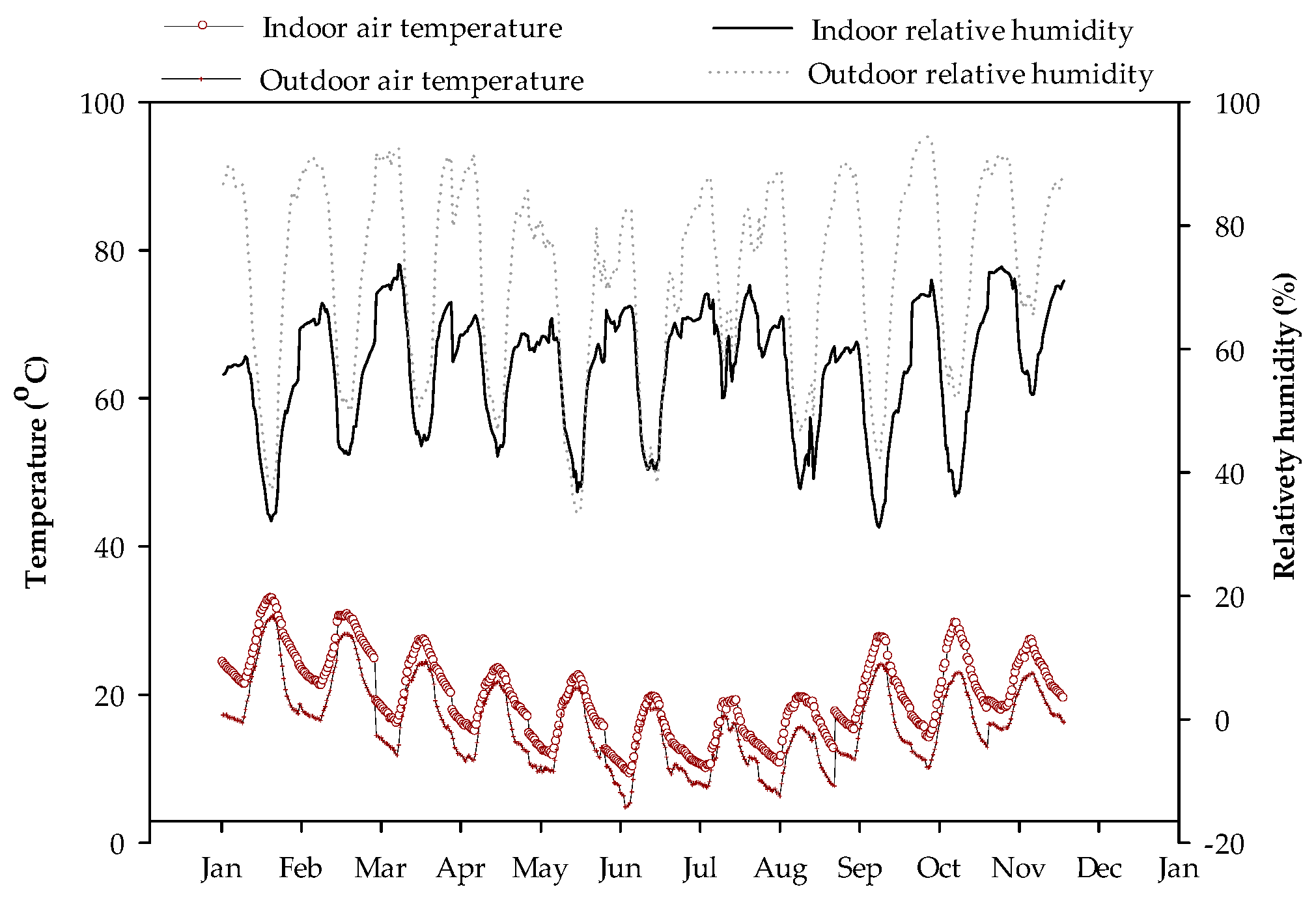
The good intention of the South Africa government to provide decent homes for low-income earners and homeless people has been overshadowed by the poor thermal performance of the houses. Despite the regulations of energy efficiency in buildings in South Africa, most low-cost housing is built ignoring energy efficiency features. As a result, low-cost householders find their homes extremely cold in winter, as revealed in the findings of this study.

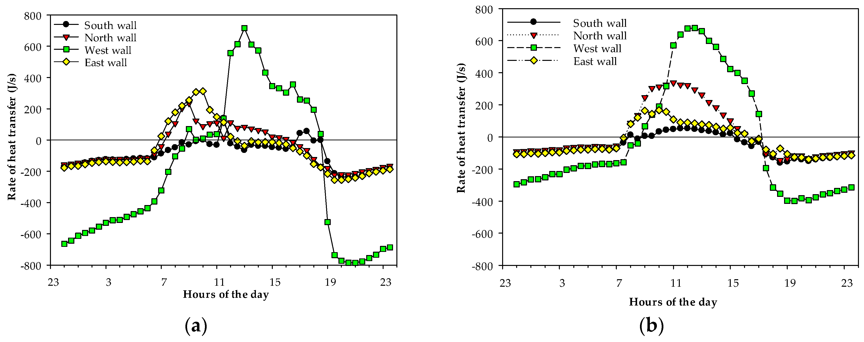
In the winter season, the indoor temperature was either out or below the SANS recommended temperature range. It was also revealed that the thermal envelope and building design play significant roles in the indoor weather conditions of the house. The components of the thermal envelope show little or no resistance to the outdoor weather conditions. As a result, the indoor temperature closely follows the outdoor temperature with a time lag of 2 h. The findings of this study also indicate that occupants (SASSA child grant dependence) will spend approximately twice their monthly income to achieve thermal comfort indoors. The poor thermal behavior of the low-cost housing also has a negative impact on the country’s carbon footprint. An average of 0.51 ton of CO₂ gas will be emitted to supply the monthly heating energy that is required in the winter seasons. Likewise, 4.30 kg and 2.08 kg of SO₂ and NO₂, respectively, will also be emitted.

A lasting solution to the poor thermal performance of low-cost housing is required. This can be achieved through strict practice of the SANS regulation of energy efficiency in building. A formal training to inform local builders about the SANS building regulation is also encouraged. In addition, promoting and enforcing the use of thermal insulation materials in houses (low-cost housing) will not only bring about energy savings but will also provide year-round indoor thermal comfort.

References

1. Global Alliance for Buildings and Construction. Towards Zero-Emission Efficient and Resilient Buildings: Global Status Report 2016; United Nation Environment Programme: Paris, France, 2016; pp. 1–32. [Google Scholar]
2. U.S. Energy Information Administration. International Energy Outlook 2016; Energy Information Administration: Washinton, DC, USA, 2016; Volume 0484.
3. Estiri, H. Building and household X-factors and energy consumption at the residential sector. A structural equation analysis of the effects of household and building characteristics on the annual energy consumption of US residential buildings. Energy Econ. 2014, 43, 178–184. [Google Scholar] [CrossRef]
4. González-Eguino, M. Energy poverty: An overview. Renew. Sustain. Energy Rev. 2015, 47, 377–385. [Google Scholar] [CrossRef]
5. World Health Organization Organization. Fuel for Life: Household Energy and Health; World Health Organization: Geneva, Switzerland, 2006. [Google Scholar]
6. Dear, K.B.G.; McMichael, A.J. The health impacts of cold homes and fuel poverty. BMJ 2011. [Google Scholar] [CrossRef] [PubMed]
7. Ormandy, D.; Ezratty, V. Health and thermal comfort: From WHO guidance to housing strategies. Energy Policy 2012, 49, 116–121. [Google Scholar] [CrossRef]
8. Rademaekers, K.; Yearwood, J.; Ferreira, A.; Pye, S.; Ian Hamilton, P.; Agnolucci, D.G.; Karásek, J.; Anisimova, N. Selecting Indicators to Measure Energy Poverty; European Commission: Brussels, Belgium, 2016; p. 130. [Google Scholar]
9. Wright, C. Profitable Investment in Energy Poverty and Environmental Sustainability; London School of Economics: London, UK, 2008. [Google Scholar]
10. Klunne, W. Energy Efficient Housing in South Africa; Boiling Point: Bellevue, WA, USA, 2002; p. 46. [Google Scholar]
11. Sustainable Energy Africa. Tackling Urban Energy Poverty in South Africa; Heinrich Boell Foundation: Cape Town, South Africa, 2014; pp. 1–12. [Google Scholar]
12. Department of Energy. A Survey of Energy-Related Behaviour and Perceptions in South Africa: The Residential Sector Report 2012; DOE: Pretoria, South Africa, 2012; pp. 1–118.
13. Department of Energy. A Survey of Energy Related Behaviour and Perceptions in South Africa: The Residential Sector Report 2013; Department of Energy: Pretoria, South Africa, 2013; pp. 1–142.
14. Inglesi, R. Aggregate electricity demand in South Africa: Conditional forecasts to 2030. Appl. Energy 2010, 87, 197–204. [Google Scholar] [CrossRef]
15. Eskom. Free Basic Electricity. Available online: http://www.eskom.co.za/news/Pages/Apr18.aspx (accessed on 19 February 2017).
16. Department of Energy. State of Renewable Energy in South Africa; DOE: Pretoria, South Africa, 2015.
17. Makaka, G.; Meyer, E.L.; Mamphweli, S.; Simon, M. The Behaviour of Low-Cost Passive Solar Energy Efficient House, South Africa; InTech: Rijeka, Croatia, 2008. [Google Scholar]
18. Donaldson-Selby, G.; Hill, T.; Korrubel, J. Photorealistic visualisation of urban greening in a low-cost high-density housing settlement, Durban, South Africa. Urban For. Urban Green. 2007, 6, 3–14. [Google Scholar] [CrossRef]
19. Klunne, W.E. Energy efficient housing to benefit South African households. Boil. Point 2002, 48, 27–29. [Google Scholar]
20. Energy Information Administrator. South Africa International Analysis U.S. Energy Information Administration (EIA). Available online: https://www.eia.gov/beta/international/analysis.cfm?iso=ZAF (accessed on 20 February 2017).
21. Nejat, P.; Jomehzadeh, F.; Taheri, M.M.; Gohari, M.; Muhd, M.Z. A global review of energy consumption, CO2 emissions and policy in the residential sector (with an overview of the top ten CO2 emitting countries). Renew. Sustain. Energy Rev. 2015, 43, 843–862. [Google Scholar] [CrossRef]
22. Persson, M.L.; Roos, A.; Wall, M. Influence of window size on the energy balance of low energy houses. Energy Build. 2006, 38, 181–188. [Google Scholar] [CrossRef]
23. Goia, F.; Time, B.; Gustavsen, A. Impact of Opaque Building Envelope Configuration on the Heating and Cooling Energy Need of a Single Family House in Cold Climates. Energy Procedia 2015, 78, 2626–2631. [Google Scholar] [CrossRef] [Green Version]
24. Freire, R.Z.; Oliveira, G.H.C.; Mendes, N. Predictive controllers for thermal comfort optimization and energy savings. Energy Build. 2008, 40, 1353–1365. [Google Scholar] [CrossRef]
25. America Society of Heating, Refrigerating and Air-Conditioning Engineers (ASHRAE). Standard 55-2004, Thermal Environmental Conditions for Human Occupancy; America Society of Heating, Refrigerating and Air-Conditioning Engineers: Atlanta, GA, USA, 2004. [Google Scholar]
26. Butera, F.M. Chapter 3—Principles of thermal comfort. Renew. Sustain. Energy Rev. 1998, 2, 39–66. [Google Scholar] [CrossRef]
27. America Society of Heating, Refrigerating and Air-Conditioning Engineers (ASHRAE). 2009 ASHRAE Handbook: Foundamental; America Society of Heating, Refrigerating and Air-Conditioning Engineers: Atlanta, GA, USA, 2009; Volume 30329. [Google Scholar]
28. Fanger, P.O. Thermal Comfort. Analysis and Applications in Environmental Engineering; Danish Technical Press: Copenhagen, Denmark, 1970. [Google Scholar]
29. Lin, Z.; Deng, S. A study on the thermal comfort in sleeping environments in the subtropics—Developing a thermal comfort model for sleeping environments. Build. Environ. 2008, 43, 70–81. [Google Scholar] [CrossRef]
30. International Organization for Standardization (ISO). ISO 7730: Ergonomics of the thermal environment Analytical determination and interpretation of thermal comfort using calculation of the PMV and PPD indices and local thermal comfort criteria. Management 2005, 3, 605–615. [Google Scholar]
31. E.N. ISO 7730:1994. Moderate Thermal Environment PMV PPD indices Specification Condition Thermal Comfort; International Organization for Standardization: Geneva, Switzerland, 1994. [Google Scholar]
32. International Organization for Standardization (ISO). Moderate Thermal Environments: Determination of the PMV and PPD Indices and Specification of the Conditions for Thermal Comfort = Ambiances Thermiques Modérées: Détermination Des Indices PMV Et PPD et Spécification des Conditions de Confort Thermique; International Organization for Standardization: Geneva, Switzerland, 1984. [Google Scholar]
33. SABS. SANS 204:2011—South African National Standard: Energy Efficiency in Buildings; SABS Standards Divisio: Pretoria, South Africa, 2011; Volume 1. [Google Scholar]
34. Kalogirou, S. Chapter 6—Solar Space Heating and Cooling; Elsevier: Amsterdam, The Netherlands, 2014. [Google Scholar]
35. Büyükalaca, O.; Bulut, H.; Ylmaz, T. Analysis of variable-base heating and cooling degree-days for Turkey. Appl. Energy 2001, 69, 269–283. [Google Scholar] [CrossRef]
36. Eskom. Tariff and Charges Booklet. Eskom Holdings SOC LTD 2016. Available online: http://www.eskom.co.za/CustomerCare/TariffsAndCharges/Documents/tariff booklet proof1.pdf (accessed on 6 March 2017).
37. Garg, A.; Kazunari, K.; Pulles, T.; IPCC—Intergovernmental Panel on Climate Change. 2006 IPCC Guidelines for National Greenhouse Gas Inventories, Volume 2: Energy; IPCC: Geneva, Switzerland, 2006; Volume 2. [Google Scholar]
38. EB41—Annex 11: Methodological Tool: Tool to Calculate Project or Leakage CO2 Emissions from Fossil Fuel Combustion v. 02. Available online: https://cdm.unfccc.int/methodologies/PAmethodologies/tools/am-tool-03-v2.pdf (accessed on 11 March 2017).
39. Conradie, D.C.U. South Africa’s climatic zones: Today, tomorrow. In Proceedings of the International Green Building Conference and Exhibition: Future Trends and Issues Impacting on the Built Environment, Sandton, South Africa, 25–26 July 2012; pp. 1–9.
40. The Thermal Insulation Association of Southern Africa. The Guide to Energy Efficient Thermal Insulation in Buildings; Association of Architectural Aluminium Manufacturers of South Africa: Pretoria, South Africa, 2010; pp. 1–64. [Google Scholar]
41. South Africa Weather Service. Climate South Africa. Available online: ftp://ftp.weathersa.co.za (accessed on 1 January 2013).
42. Montgomery, K.K. Type N versus type K thermocouple comparison in a brick kiln. Temp. Meas. Control Sci. Ind. 1992, 6, 601–605. [Google Scholar]
43. Campbell Scientific. Instruction Manual. HMP60 Temperature and Relative Humidity Probe; Campbell Scientific: Logan, UT, USA, 2010; pp. 1–18. [Google Scholar]
44. Kerr, J.P.; Thurtell, G.W.; Tanner, C.B. An integrating pyranometer for climatological observer stations and mesoscale networks. J. Appl. Meteorol. 1967, 6, 688–694. [Google Scholar] [CrossRef]
45. Campbell Scientific. Instruction Manual. 03001 R.M. Young Wind Sentry Set 03101; Campbell Scientific: Logan, UT, USA, 2013; pp. 1–34. [Google Scholar]
46. South Africa Weather Service. How are the dates of the four seasons worked out? WeatherSA. 2012. Available online: http://www.weathersa.co.za/learning/weather-questions/82-how-are-the-dates-of-the-four-seasons-worked-out (accessed on 4 May 2013).
47. Eskom. Tariff and Charges Booklet. Eskom Holdings SOC LTD 2015. Available online: http://www.eskom.co.za/CustomerCare/TariffsAndCharges/Pages/Tariffs_And_Charges.aspx (accessed on 6 March 2017).
48. Hoyt, T.; Schiavon, S.; Piccioli, A.; Moon, D.; Steinfeld, K. CBE Thermal Comfort Tool; Center Built Environment University: Berkeley, CA, USA, 2013. [Google Scholar]
49. Szokolay, S.V. Introduction to Architectural Science: The Basis of Sustainable Design; Routledge: Abingdon, UK, 2014. [Google Scholar]
50. Al-Jabri, K.S.; Hago, A.W.; Al-Nuaimi, A.S.; Al-Saidy, A.H. Concrete blocks for thermal insulation in hot climate. Cem. Concr. Res. 2005, 35, 1472–1479. [Google Scholar] [CrossRef]
51. National Energy Regulatior of South Africa. Reason for Decision; Eskom Landlight 60A and 20A Tariffs; National Energy Regulatior of South Africa: Pretoria, South Africa, 2016.
52. South African Social Sercurity Agency. You and Your Grants 2016/17; South African Social Sercurity Agency: Pretoria, South Africa, 2016.
53. BP. BP Statistical Review of World Energy—Full Report; BP: London, UK, 2016. [Google Scholar]
54. Eskom. Environmental Implications of Using or Saving Electricity; Integrated Results Presentation; Eskom Holdings Limited: Johannesburg, South Africa, 2014; Available online: http://integratedreport.eskom.co.za/supplementary/app-environmental.php (accessed on 1 January 2016).
55. Eskom. Integrated Report 2014; Eskom Holdings SOC LTD: Johannesburg, South Africa, 2014. [Google Scholar]
Figure 1. (a) Photo of the low-cost house used as case study (typical South African low-cost housing); and (b) floor plan diagram of the house.
Sustainability 09 00425 g001
Figure 2. Typical low cost house and floor plan.
Sustainability 09 00425 g002
Figure 3. (a) Indoor and outdoor temperature and relative humidity distribution on a typical summer day; and (b) indoor and outdoor temperature and relative humidity distribution on a typical winter day.
Sustainability 09 00425 g003
Figure 4. (a) A typical summer day solar radiation distribution; and (b) wind rose profile of the house location in the summer season.
Sustainability 09 00425 g004
Figure 5. (a) Typical winter day solar radiation distribution; and (b) winter season wind rose profile of the house location.
Sustainability 09 00425 g005
Figure 6. (a) Loose windows even while closed; (b) space between the window and it frame; (c) cracks between the roof and the building wall; and (d) opening between the door and its frame.
Sustainability 09 00425 g006
Figure 7. (a) Average summer daily indoor temperature and relative humidity response to the components of thermal envelope surface temperature; and (b) average winter daily indoor temperature and relative humidity response to the components of thermal envelope surface temperature.
Sustainability 09 00425 g007
Figure 8. (a) Summer season rate heat transfer through perimeter walls; and (b) winter season rate heat transfer through perimeter walls.
Sustainability 09 00425 g008
Figure 9. Average monthly indoor air temperature and monthly degree-hours of the house.
Sustainability 09 00425 g009