
Analysis of the Dynamic Evolutionary Behavior of American Heating Oil Spot and Futures Price Fluctuation Networks


1
Energy Development and Environmental Protection Strategy Research Center, Jiangsu University, Zhenjiang 212013, China
2
School of Mathematical Science, Nanjing Normal University, Nanjing 210042, China
3
Department of Mathematics, Nanjing Normal University Taizhou College, Taizhou 225300, China
*
Author to whom correspondence should be addressed.
Sustainability 2017, 9(4), 574; https://doi.org/10.3390/su9040574
Submission received: 23 January 2017
/
Revised: 22 March 2017
/
Accepted: 6 April 2017
/
Published: 10 April 2017
(This article belongs to the Special Issue Selected Papers from 7th Annual Conference of Energy Economics and Management)
Abstract
:Heating oil is an extremely important heating fuel to consumers in northeastern United States. This paper studies the fluctuations law and dynamic behavior of heating oil spot and futures prices by setting up their complex network models based on the data of America in recent 30 years. Firstly, modes are defined by the method of coarse graining, the spot price fluctuation network of heating oil (HSPFN) and its futures price fluctuation network (HFPFN) in different periods are established to analyze the transformation characteristics between the modes. Secondly, several indicators are investigated: average path length, node strength and strength distribution, betweeness, etc. In addition, a function is established to measure and analyze the network similarity. The results show the cumulative time of new nodes appearing in either spot or futures price network is not random but exhibits a growth trend of straight line. Meanwhile, the power law distributions of spot and futures price fluctuations in different periods present regularity and complexity. Moreover, these prices are strongly correlated in stable fluctuation period but weak in the phase of sharp fluctuation. Finally, the time distribution characteristics of important modes in the networks and the evolution results of the topological properties mentioned above are obtained.
1. Introduction
Heating oil is a low viscosity, liquid petroleum product used as a fuel oil for furnaces or boilers in buildings. As EIA (U.S. Energy Information Administration) reported, there are about six million households in the United States using heating oil as their main heating fuel at present, and mostly used in the northeastern United States. Heating oil is refined from crude oil at a 25% yield, thus its prices are generally closely related to fluctuations in crude oil prices [1,2], also depending on the amount of fuel purchased. Unlike natural gas which is purchased on demand, heating oil must be purchased in advance, and usually with a large amount, which has brought a considerable burden to lots of American families. In addition, heating oil prices paid by consumers can vary for a variety of reasons: seasonality in the demand for heating oil, competition in local markets and regional operating costs. As a result, heating oil prices have changed significantly over time, with changes occurring every season (due to fluctuations in demand for space heating throughout the year), weekly or even daily (due to fluctuations in world crude oil prices) [3]. The volatility of prices over time makes it difficult for many households to manage the purchase effectively. Therefore, exploring the volatility of heating oil prices in the spot and futures markets can help to provide a scientific basis to quantify the uncertainties in the market and avoid market risks.
In recent years, many researchers at home and abroad have done research on the modeling, prediction, influence of heating oil price volatility and the guiding relationship among different markets. For example, in terms of the prices of heating oil, Porter [4] proposed a model for the production of distillate fuel oil to determine the impact of production decisions on the price of heating oil, and found that these decisions did influence the prices of heating oil a lot. However, this study was flawed in not delving into the fluctuation law of prices, so it could not perform out-of-sample forecasts for heating oil prices. Wang et al. [5] introduced an X-11-ARIMA seasonal adjustment method, which was used to analyze the seasonal fluctuation of international heating oil prices and explore law of oil price movement, and then to provide decision support for China’s oil imports. In addition, in order to further study the internal connection of heating oil prices, many researchers carefully divided it into spot prices and futures prices, and examined the relationship between them. For instance, Hammoudeh et al. [1] investigated the time-series characteristics of the daily spot and futures prices of heating oil in five commodity trading centers within and outside the United States, and reached a conclusion that there were strong bi-directional causalities between spot and futures prices, with the spot price having the upper hand in terms of volatility spillover effects in the New York Mercantile Exchange (NYMEX) heating market. Chinn et al. [6] explored the relationship between spot prices and futures prices for energy commodities (crude oil, gasoline, heating oil and natural gas) and obtained that futures prices are unbiased predictors of heating oil prices. Besides, time series models (relating a commodity price to lagged own prices, and estimated errors) did usually fare worse than commodity futures prices as forecasts. Wang et al. [7] selected the yield data sequence of international heating oil futures prices, demonstrated that energy futures market was a complex nonlinear system using phase space reconstruction technology [8], then they concluded that a long-term equilibrium relationship existed between heating oil futures prices and spot prices, and futures prices bore 80.30% of the price discovery function.
A great deal of existing literature usually uses statistical and econometric models to quantify the price fluctuations of heating oil. Taking into account the existence of stable fluctuations period and sharp fluctuations period in the fluctuations of energy prices, thus exploring the evolution characteristics of topological dynamics that change with time will be able to provide more reference for price decision makers, while the complex network is a useful tool for studying the network topology structure. With the development of complex network theory, complex network analysis methods have been widely used in many fields such as international trade, social science and geography etc. [9,10,11,12,13,14,15,16,17,18]. At present, complex networks have become a new approach to energy research [19,20,21,22,23,24,25,26,27,28,29]. For example, in the research field of energy prices, An [28] designed a complex network method to research some dynamic characteristics of the linkage between crude oil futures and spot prices based on the data of the West Texas Intermediate crude oil futures prices and Daqing (China) crude oil spot prices on 25 November 2002 to 22 March 2011. Wang [29] built the directed weighted networks of international crude oil and gasoline prices and analyzed the evolution law of new nodes in the prices networks. In contrast, An denoted the fluctuation states of the co-movement modes between the crude oil futures and spot prices by three symbols, while Wang converted the crude oil and gasoline price volatility sequences into the characters composed by five symbols, which can better reflect complexity of energy price fluctuations. At the same time, these studies indicate that the complex network is indeed a good way to study fluctuations.
In view of the previous literature on the research of heating oil, price fluctuations often adopted the traditional mathematical analysis method, which cannot effectively reflect the complexity of price volatility and dynamic evolution characteristics changing with time. Therefore, this paper combines the theory of complex network which is a popular method to study the fluctuation behavior of heating oil prices in America.
Three main innovations of this paper are: (1) It selects the data with larger time span to establish complex network models of the U.S. heating oil spot and futures prices, and divides periods according to the different states of price fluctuation. Then the structures and topological properties of the spot and futures prices networks are investigated from overall and local point of view respectively, with more contrast and explanatory; (2) It designs a similarity function of heating oil price fluctuation network to analyze the dependency behavior of spot and futures price fluctuations in different periods, and compares with the calculation results of Spearman rank correlation coefficient and Pearson correlation coefficient to highlight its effectiveness and superiority; (3) It initially explores the forward-looking of price behavior in terms of occurrence time of new nodes in futures market.
This paper is structured as follows: Section 2 introduces the data and methods, namely the source and coarse graining process of data [30], period division process, the construction of complex network models and some concepts of network topological properties. Section 3 outlines the corresponding results and analysis. Finally, the main conclusions and prospects are given in Section 4.
2. Data and Methods
2.1. Sources and Processing of Data
The data selected are from New York Harbor No. 2 Heating Oil Spot Price FOB (Dollars per Gallon) and New York Harbor No. 2 Heating Oil Future Contract 1 (Dollars) considering the period 2 June 1986–1 July 2016, which can be obtained by EIA. In addition, the trends of fluctuations of heating oil spot and futures prices for the past three decades are showed in Figure 1.
At first, the heating oil spot and futures price sequences are denoted as and respectively. For the U.S. heating oil spot and futures prices, we are concerned about the information of price changes, that is, the daily price position. As for continuous spot price sequence of heating oil, assuming that is the current price, is the previous prices, then the fluctuation sequence of heating oil spot prices can be expressed as . At the same time, the fluctuation sequence of heating oil futures prices can be written as .
Let the average fluctuation sequence of heating oil futures prices is , and , it means heating oil prices fell steadily when , the prices rise sharply when , at the same time, it means heating oil prices rose steadily if , and a steady fall if . Besides, it means a sharp fall in heating oil prices when . The coarse-grained treatment of the sample data omits small levels of detail, and the validity of conclusions largely depends on the accuracy of coarse graining processing. In order to reveal the law between heating oil spot prices and futures prices of America more clearly, the symbols should not be chosen too many. Next we make every variable value of correspond to a certain letter, then get the heating oil price fluctuations sequence represented by letters, that is, each value of with a symbol of corresponding to,
where , , , and represent the states of sharp rise, steady rise, stabilization, steady fall and sharp fall respectively. According to the method mentioned above, it is feasible to convert the fluctuation sequence of American heating oil spot prices into the corresponding symbol sequence:
Similarly, the fluctuation sequence of heating oil futures prices can also be converted as below:
2.2. Period Division
, , , and those mean the occurrence probability of , , , and respectively are calculated for each period of 12 months based on the results of data processing in Section 2.1. The probability evolution of each symbol is shown in Figure 2a. As we can see, the occurrence probability of steady volatility state is the smallest, which is generally between 0 and 0.1 in the spot price fluctuations of heating oil. While the occurrence probability of the sharp rise state , the sharp fall state , the steady rise state and the steady fall state appear alternately around 2004. In order to further distinguish the periods of sharp ups and downs, as well as steady ups and downs, we carry out the following calculation:
where represents the occurrence probability of a steady rise and fall of heating oil spot prices, represents the occurrence probability of a sharp rise and fall of heating oil spot prices, and then the evolution images of and are obtained, as shown in Figure 2b. It illustrates that the probability of a sharp state of ups and downs begins to exceed that of a steady state of ups and downs, indicating the state of heating oil spot prices fluctuations has changed. We divide the period from 2 June 1986 to 26 February 2004 as the stable fluctuation period of heating oil spot prices; 26 February 2004–1 July 2016 is divided into the volatile fluctuation period of heating oil spot prices, which can be further divided into a sharp rise period and a sharp fall period. Therefore, we do further research during the volatile fluctuation period and make the following calculation:
where and represent the occurrence probability of the sharp rise and sharp fall respectively, as shown in Figure 2c. And it can be clearly seen that the volatile fluctuation period of heating oil spot prices is divided into six different periods according to the different proportions of rising and falling. To sum up, the heating oil spot price fluctuations can be divided into seven periods (see Table 1).
Similarly, we can get the evolution of heating oil futures price fluctuations, as shown in Figure 3. As can be seen from Figure 3, the heating oil futures price fluctuations could be divided into six periods (see Table 2).
From the above results, the rising and falling states of both spot prices and futures prices change at around 2004. According to the Futures Daily reported that the supply and demand of the international crude oil was in a state of tension in 2004, many core crude oil import ports and oil refining centers were attacked by the hurricane in September and October 2004, which made lots of refineries close down, and caused a serious impact to increase the inventories of heating oil and the supply of crude oil. Observing the stocks of America heating oil since 2000, which has reached its lowest level while absolute high demand for near five years in 2004, thus making it become deteriorated for the contradiction between supply and demand of the U.S. heating oil market, which determines its price from the stable fluctuation period into the volatile fluctuation period.
2.3. Complex Network Model
2.3.1. Complex Network Analysis Methods
Under normal circumstances, the trading days of the U.S. heating oil futures and spot market are five days a week, so we are on the basis of getting the spot price symbol sequence and futures price symbol sequence , using five symbols to represent price fluctuations for five days, then making them compose a sequence of symbols and defining this as a mode, and then choosing one day for the step to do data sliding. As a result, 7539 volatility modes of spot prices and futures prices (including the same mode) have been obtained respectively. Since the modes are formed by sliding the data, the former mode is the basis for the formation of the latter one, and the modes are directional and transitive. Therefore, it is possible to build a directional weighted network of heating oil prices with each fluctuation mode as the node, the directional transformation between the modes as the edge and the transformation times as the weight. We take the spot price fluctuation network of heating oil as an example, and its construction process is shown in Table 3.
In Table 3, the fluctuating modes change with the sliding of the window, so we can get the volatility modes sequence , and construct the directional weighted network based on these modes. Thus, each node represents a fluctuating state of the spot prices or futures prices. For example, Table 3 shows that transforms into , which indicates both modes and are nodes in the network and there is a directed edge between them. If there are 3 times for to convert into in the whole process, it means that the weight of this edge is 3. As a result of the coarse-grained processing, some fluctuating modes appear repeatedly, then 1501 different fluctuation modes of spot prices and 1446 different fluctuation modes of futures prices are obtained after the deletion finally.
2.3.2. HSPFN and HFPFN in Different Periods
In order to facilitate observation and comparison, we select some data of the same length in each period to construct the price fluctuation network of heating oil in the process of drawing, while analyzing the results of full-data network in each period. Then the spot price fluctuation network of heating oil and different periods of that have been gained, as shown in Figure 4. The futures price fluctuation network of heating oil and different period of that, as shown in Figure 5. In Figure 4a and Figure 5a, the solid line represents the positive direction, the dotted line shows the opposite direction, and the size of a node denotes the size of its weight. In the three-dimensional images of price fluctuation networks in different periods, red shows the closest nodes, lime green represents the nodes with the minimum angle, cyan indicates the nodes with the shortest line, and blue denotes the nodes with the longest line in the layout. Besides, yellow signifies the number of crossings, pink represents the node closest to the line. For example, in Figure 4b, the closest nodes are and , the distance between them is 0.06847. The minimum angle is from node to , then to , and the angle is 4.9082. The shortest line is the connection between and , with a length of 0.0733. The longest line is the connection between and , and the length is 0.3006. At the same time, the number of crossings is 40, and the closest node to line is which leaves the distance between nodes and at 0.0007.
It can be seen from Figure 4a and Figure 5a that the connection between nodes is very complex in HSPFN and HFPFN. From the view of different periods, there are different three-dimensional network structures for the spot and futures price volatility networks at different times. For the above characteristics, comparative analysis one by one in the following sections will be made.
First of all, we may as well consider HSPFN and HFPFN (see Figure 4a and Figure 5a). According to the method of constructing networks in Section 2.3.1, the price fluctuation mode of heating oil is the 5-character mode that is composed of five types of symbols. Therefore, there should be 3125 () different modes in theory. However, as previously discussed, there are 1501 and 1446 different fluctuation modes (nodes) in HSPFN and HFPFN, and the numbers of modes appearing in different fluctuation periods are 211~1471 and 204~1397 respectively. Next, from the point of view of node number, which in HFPFN is less than that in HSPFN, thus it can be inferred that the fluctuation of heating oil spot prices is more complicated.
2.4. Dynamic Characteristics of Heating Oil Price Fluctuation Networks
Next, we analyze the fluctuations of spot prices and futures prices from the perspective of global network and local network, and then find out the dynamic evolution mechanism within price fluctuations.
2.4.1. The Average Path Length
A simple path between two nodes and that experiences the least number of edges (edges are different) is called a geodesic. The edge number of geodesics is called the distance between nodes and . The diameter [9] of the network is defined as the maximum of all distances ,
2.4.2. Strength and Strength Distribution
The key status of nodes can be explained by their degree and strength in the complex network theory. Since what we established were the directional weighted networks for the heating oil spot and futures price fluctuations, thus the strength and strength distribution of nodes need to be discussed in this section. In the un-weighted network, the degree of a node mainly reflects the connection between the node and other nodes. However, the strength of a node not only reflects the connection between the node and other nodes, but also shows the weight of the edge between two nodes. In another word, strength is a weighted statement of degree, which measures the sum of the weights of all the edges for a given node. The strength of node is divided into the out-strength and in-strength, but the in-strength of node represents the number of times that other nodes convert to it, and the out-strength is in contrast. The in-strength and out-strength of nodes [9] are calculated as follows:
where denotes the weight of the edge connecting nodes to , and it means that to are not connected if .
The strength distribution of nodes [28] is defined by
where is the strength and is the sum of the strength of all nodes. The greater the strength and strength distribution of a mode are, the more times it will transform into other modes (including the current mode), which means a higher probability and importance of it existing in the network. In addition, the network is a scale-free network if the strength distribution of it can be fitted by the power-law distribution described by
which is equivalent to
where is the proportionality constant, is the power exponent, the greater the value of is, the stronger the power-law distribution of the network will be.
According to the construction method of the price fluctuation network model in Section 2.3.1, these nodes are connected in time order, hence the out-strength and in-strength of nodes are the same except for the first and the last one. Next, for convenience of operation and description, we only consider the in-strength of nodes, and both of them will be narrated as strength in the following.
2.4.3. Betweeness Centrality
In some large-scale networks, the status of different nodes is different. For example, in the process of damaging network nodes, the network will be paralyzed if some nodes are damaged. To measure the importance of a node, its degree can certainly be used as a measure, but not entirely. Another metric called betweenness [28,29] needs to be defined, which is a global feature measure that reflects the influence and role of nodes or edges in the whole network. The shortest path between non-adjacent nodes and in the network will pass through some nodes, if a node is traversed by many other shortest paths, it means the node is important, and its influence or importance can be expressed by the betweenness [32], in the directed network is defined as follows
where represents the shortest path number of node to node , and is the number of the shortest path from node to node that passing through node . Thus, the betweenness of node is the proportion of all the shortest paths passing through it in the network.
2.4.4. Clustering Coefficient
The clustering coefficient of nodes mainly reflects the closeness of adjacent nodes. This kind of natural clustering of complex networks can be described quantitatively by the average clustering coefficient. In graph theory, the average clustering coefficient refers to the average probability of two nodes connecting to the same node in the network, which is usually used to characterize the local structure of a network. In order to derive the definition of average clustering, we may as well define the clustering coefficient first. In a directed weighted network, the clustering coefficient [29,33] of a node is defined as
where and denote the edge weights of two nodes and two nodes , respectively. represents the node strength, and . Besides, denotes the degree of node , and indicates the total number of triangles in the network that contain .
Next the average clustering coefficient of a network is obtained by averaging the clustering coefficient over the whole network [34], which is defined as
Apparently , if and only if the clustering coefficients of all nodes in the network are zero; if and only if the clustering coefficients of all nodes in the network are 1, then the network is globally coupled at this time. That is, any two nodes in the network are directly connected.
3. Results and Analysis
3.1. Regularity Analysis for the Appearance of New Nodes
Based on the networks of spot and futures prices fluctuation in different periods in Section 2.3.2, we study the emergence regularity of new nodes from the view of the cumulative time interval, as shown in Figure 6.
Figure 6a shows that the red solid line indicates the equal time interval curve, and it can be seen that the cumulative time interval of new nodes is not equidistant but gradually increasing in a straight line in the evolution of HSPFN and HFPFN. The cumulative time of new nodes in HSPFN and HFPFN is regressed by the least square method, and the corresponding regression equations are as follows: and , respectively, of which 0.988 and 0.981 are the values of their trend line correlation coefficient . It shows a higher credibility of the results, and indicates that the accumulation time of new nodes in HSPFN and HFPFN increases linearly, which presents a good regularity. This regularity reflects the temporal variation of spot and future prices can be forward-looking. For instance, in the futures price fluctuation network of heating oil, it can be projected that the 1700th new node will appear on 7 September 2018 according to this method, the emergence time of the 1800th new node will be on 3 August 2020. From the comparison of the network nodes, the length of new nodes’ time interval in the HFPFN (indicated by green “○” in Figure 6a) is larger than that in HSPFN (indicated by the blue “Δ” in Figure 6a), indicating that when the data are based on the same length to build the network, the number of network nodes in HSPFN will be more than that in HFPFN, which also explains the evolution of HSPFN is more complex to some extent.
From the perspective of different periods, Figure 6b shows the cumulative time intervals between HSPFN and HFPFN in the stable and sharp fluctuation periods. It can be noticed that their cumulative time intervals also pose a good regularity, that is, which show a growth trend of straight line. Similarly, the regression equations of the cumulative time intervals of new nodes appearing in the stable fluctuation period and the sharp fluctuating period of HSPFN are respectively and , and the trend line correlation coefficient are 0.956 and 0.935, respectively. However, the corresponding regression equations in HFPFN case are and separately, with their trend line correlation coefficient are 0.945 and 0.922. Therefore, it is easy to notice that the reliability of their results is high, indicating that either in the period of sharp fluctuation or stable fluctuation, the accumulation time of new nodes appearing in HSPFN and HFPFN is not a disorder but a high degree of rectilinear growth trend. At the same time, for HSPFN, the cumulative time interval of new nodes in the stable fluctuation period is longer than that in the sharp fluctuation phase (see the upper part of Figure 6b), the same is true of sharp fluctuation period (see the second part of Figure 6b), and the two are very similar.
To sum up, new nodes appearing in the heating oil price fluctuation networks mean some nodes of abnormal volatility (different from the previous state of volatility), indicating that the fluctuation of heating oil prices has complex non-linearity, but the cumulative time of the abnormally fluctuating price node has shown rectilinearity. Using this law can effectively identify the occurrence time of these abnormally fluctuating nodes, and make price decision-makers react in time for the arrival of a new price fluctuation sequence, thereby improve the accuracy when forecasting energy prices.
3.2. Conversion Cycle Analysis of Price Fluctuation Mode
According to the relevant definitions of the average path length in Section 2.4.1, we use the Floyd algorithm [29,35] to calculate the distance between any two nodes in the network, the results and different path length distributions are shown in Figure 7.
As shown in Figure 7a,c, the network diameter is 22 in HSPFN, the average path length of the network is 7.7834, and the distances between nodes of 6, 7, 8, 9 account for 66.28% of the total, indicating the price fluctuation modes in the HSPFN show a short-range correlation, and the conversion cycle of 7–8 days, showing that the conversion is frequent. Besides, Figure 7b,d show the HFPFN situation, the network diameter is 21, the average path length of this network is 7.7342, the distances between nodes of 6, 7, 8, 9 account for 66.52% of the total, which reveals that fluctuation modes also show a short-range related nature with a conversion cycle of 7–8 days. In contrast, is slightly smaller than , but the conversion cycles of price fluctuation modes basically the same, are 7–8 days. These properties provide a basis for predicting the periodic conversion rules of heating oil price fluctuations in the future.
Spot prices can reflect the influence of seasonal factors and other factors on heating oil prices, so we may consider from different periods (see Figure 8a) for the spot price fluctuation network. In the stable fluctuation period, the network diameter is 25, the average path length is 9.1874, indicating that the conversion cycles of spot price fluctuation modes are 9–10 days. In addition, the distances between nodes are 7, 8, 9, 10 and 11, which account for 67.50% of the total number. In the period of sharp fluctuation, the network diameter is 26, and the average path length is 8.5679, which means the transformation periods of this case are 8-9 days. Besides, the distances between nodes are 6, 7, 8, 9, and 10, accounting for 70.05% of the total. By comparing the results of different periods, a longer diameter and a shorter volatility cycle can be found during the sharp fluctuation period for HSPFN. As the price volatility period is often caused by some significant impact of the incidents, thus our results can show that the occurrence of emergencies may accelerate the conversion cycle of price volatility.
As for HFPFN, taking the same angle of different periods to consider (see Figure 8b). In the period of stable fluctuation, the network diameter is 30, the average path length is 8.9346, which indicates that the transition periods of fluctuation modes in futures prices are 8–9 days during the stable fluctuation period. In addition, the distances between nodes are 7, 8, 9 and 10, accounting for 58.24% of the total number. However, in the sharp fluctuation period, the network diameter is 21, the average path length is 8.3546, indicating that the conversion cycles of fluctuation modes in futures prices are 8–9 days. The distances between nodes are 6, 7, 8, 9 and 10, which account for 71.91% of the total. These show unexpected events on the conversion cycle of futures price fluctuations with little effect due to futures prices sometimes fail to make timely adjustments to the impact of emergencies.
The above analysis demonstrates that the heating oil spot and futures prices have a cyclical character from the whole point of view. That is, a change occurs in seven to eight days, and this change is likely to be wave modes occurred in the past. This phenomenon may due to some factors that affect the change of wave modes, and the volatility modes are sensitive to the influence of these factors. For instance, the trading days of heating oil are five days of a week, which may cause consumers to psychologically accept or reject such rules, and further influence the actual transaction price and trading volume, resulting in price volatility of a short period to change around a certain mode emerged in the past. Besides, it is respectively the mutual transformations between the 1501 and 1446 different modes that constitute complicated network structures in HSPFN and HFPFN established in this paper, that is why repetitive modes are generated. In another way, the conversion cycle of spot prices during the stable fluctuation period is different from that during the violent fluctuation period, but the difference is not significant, which reflects the impact of factors such as the occurrence of sudden events, changes in the natural environment and national policies on the volatility of spot prices. In terms of futures prices, the conversion cycle maintains consistency during different fluctuation periods. This shows that futures prices fail to make sensitive response to sudden situation, reflecting the difference between expectation and reality to a certain degree. In short, not only the early warning of heating oil price fluctuation can be provided according to the periodicity of spot price and futures price fluctuation, but also it reflects complex intrinsic dynamic characteristics of heating oil prices.
3.3. Analysis of Strength and Strength Distribution of Nodes
In order to further reveal the time distribution characteristics of important modes and the power-law distribution of some networks in different periods, the strength and cumulative strength distribution of nodes are investigated in the following.
As shown in Figure 9, the left coordinate represents the node strength and the right coordinate represents the cumulative strength distribution of nodes. Furthermore, most nodes in the heating oil spot and futures price fluctuation networks are small in strength, only a small number of nodes are large, which is a typical characteristic of the scale-free network. For HSPFN (see Table 4), there are 1501 nodes in the network, of which 31 nodes are more than 40 in strength, accounting for 25.80% of the total strength, namely the sum of strength of 2.07% nodes is 25.80% of the total strength. For HFPFN (see Table 4), there are 1446 nodes in the network, among which there are 30 nodes with their strength exceeding 40, accounting for 28.60% of the total strength, that is, the sum of strength of 2.07% nodes are 28.60% of the total strength.
Node strength can reflect the influence or importance of nodes in the whole network to a certain extent. These nodes have been explored with their strength more than 40 in both HSPFN and HFPFN, and then their name, strength and appearing time (see Figure 10) are obtained, among which the red line indicates the positive direction, the blue line represents the opposite direction, the character signifies the name of a node, and the number on the connecting line between two nodes indicates the weight.
More clear transformation relations and the times of transformations among important nodes (nodes with strength greater than 40) are shown in Figure 11. Among which, the transformation relationship between these nodes is represented by a black solid line, and the red number on each connecting line indicates the times of conversions between two nodes. Figure 11 could facilitate the reader’s observation and understanding of the relationship between important nodes.
In Figure 10, it can be seen from the emergence time of important nodes that the nodes with large strength tend to appear earlier at first, but the nodes appear earlier are not necessarily with large strength in HSPFN and HFPFN. In the spot price fluctuation network, 31 nodes with strength greater than 40 come from the first 135 nodes in this network. Among them, node , which occurs on 27 August 1986, is the node with the largest strength, and it is the fifty-seventh node in the network. On one hand, there are 12 nodes whose strength are one before the 135th nodes in the spot price fluctuation network, where the earliest node is with emergence time on 15 July 1986, and it is the thirtieth node appearing in the spot price volatility network. Therefore, a conclusion can be drawn that the node appears earlier does not necessarily have large strength in HSPFN. There are 30 nodes with strength greater than 40 coming from the first 122 nodes in the futures price fluctuation network. Among them, the node , which appears on 14 August 1986, is the node with the largest strength. Moreover, it is the 50th node that appears in the futures price fluctuation network. On the other hand, there are 9 nodes with strength being 1 in the first 122 nodes, and the earliest node occurring on 25 July 1986, which is the 37th node in the futures price fluctuation network. Second, it can be seen from the weight of connecting line between nodes that the nodes with large strength are all closely connected in the two price fluctuation networks of heating oil. The average contribution rate of the interconnection between important nodes is 85.74% for HSPFN, while which is 87.27% for HFPFN, hence it is easy to find both the two networks have obvious positive correlation characteristics, that is to say, the nodes with large strength are inclined to connect with nodes with large strength. These above analysis shows that although the conversions of heating oil spot and futures price fluctuations are very frequent and complicated, the first 9% nodes can reflect the core volatility state, which further confirms that the price volatility of heating oil in the future is likely to be similar to that in some past periods. Therefore, studying the fluctuating state of the first 9% nodes and their transformation relationship can help the essential characteristics of price fluctuations to be described approximately.
Figure 12 presents that most nodes in the two price fluctuation networks of heating oil have small strength, whereas a small number of nodes have larger strength as a whole. The double-logarithm curves of node strength in HSPFN and HFPFN are fitted by using the least squares linear fitting method. Then the corresponding linear regression equations are and , where 0.8511 and 0.8067 respectively are the values of trend line correlation coefficient , the visible results have a high degree of credibility, indicating that the two networks obey power-law distribution as a whole, and the power indexes corresponding to 1.5108 and 1.4253, which also from one side shows these two networks are scale-free networks. At the same time, as for the scale-free network, the larger the power exponent is, the higher the power-law distribution will be. Therefore, the power-law distribution of HSPFN is higher than that of HFPFN.
From the perspective of different periods, we investigate the double-logarithmic curves of node strength in the spot and futures price fluctuation networks of heating oil in different periods according to the time division method in Section 2.2 (see Figure 13).
Similarly, the least squares fitting method is used to regress the double-logarithmic curves of node strength in two price fluctuation networks in different periods, and the corresponding fitting parameters are shown in Table 5.
Through the observation of Figure 13 and Table 5, it can be easily seen these two price fluctuation networks of heating oil follow the power-law distribution in different periods, and the power exponents of the network correspond to different values at different periods. From the whole point of view, the power exponents of the above two networks in the severe fluctuation period are both higher than that of the stationary fluctuation period, which indicates that the power-law distribution of node strength is higher in the period of severe fluctuation. However, from the change of the power exponents perspective, the power exponent increases from the first period to the sixth period and decreases from the sixth period to the seventh period in HSPFN, suggesting that the degree of power-law distribution of HSPFN increases first and then decreases. However, for HFPFN, the power exponent increases from the first to third period, and reduces from the third to fifth period, and then decreases from the period of the fifth to the sixth. This means the power-law distribution shows a trend of increasing first and then decreasing, then increasing again in HFPFN. On the other hand, it can be found by careful comparison that, whether it is in the network of heating oil spot price volatility or futures price volatility, the maximum power index and minimum power index are present in the period of sharp rise, which means that the power-law distribution is more volatile during the period of violent upswing, and more stable during the sharp decline period.
In conclusion, we can find from the above analysis that HSPFN and HFPFN are scale-free networks, and the important modes in HSPFN are mainly composed of 31 kinds at a long term, with an average contribution rate of 80%. While the important modes of HFPFN are consisted of 30 kinds, and their average contribution rate reaches 87.27%, indicating that the conversion between nodes with larger strength is more frequent. In addition, these important nodes often come from the first 9%, so the evolution of whole network can be grasped by researching the first 9% nodes. In another way, HSPFN and HFPFN of different periods are also scale-free networks, which means node strength obeys the power-law distribution. The degree of the power-distribution is higher in the period of violent fluctuation, and of great complexity and regularity for the two price networks of heating oil. This illustrates the complex intrinsic dynamics characteristics of fluctuations in heating oil prices from the side.
3.4. The Correlation between HSPFN and HFPFN
Over the years, many scholars have always believed that there is a close correlation between spot prices and futures prices of heating oil, and they conducted systematic studies [1,7]. The next section will measure the correlation between the two from the perspective of network nodes. From results above, it can be seen that the number of nodes in HSPFN and HFPFN are 1501 and 1446 respectively, and in all of these nodes, 1200 ones are identical. We do some relevant statistics about these 1200 nodes, which is reflected in Figure 14, where the strength of a node is represented by its size, the green node remarks the node coming from spot price fluctuation network, and the red node signifies the node of futures price fluctuation network. When the strength of a node in spot price network is greater than that in futures price network with the green character representation, and vice versa by red characters.
Based on above results, the similarity of two price fluctuation networks of heating oil has been calculated using following formula:
where and are the total number of nodes in HSPFN and HFPFN, is the total number of the same nodes, and , which suggests that the similarity degree of two networks reaches the highest if . By calculating, the correlation of the node strength of spot and futures price fluctuation networks is 0.7829, which shows that the similarity of these two networks is relatively high, and the interdependence between them is relatively close.
From the point of view of different periods, this part studies the relationship between the nodes of spot price fluctuation network and futures price fluctuation network in the stable fluctuation period and the violent fluctuation period based on the period division results in Section 2.2 (see Figure 15).
Figure 15 presents that there are 1061 identical nodes in the stable fluctuation period for HSPFN and HFPFN, with the network similarity of 0.6668, whereas only 876 nodes are same in that period of sharp fluctuation, the network similarity at this time is 0.1139. Therefore, the correlation between spot prices and futures prices of heating oil is complicated and the degree of correlation is very weak during the period of violent fluctuation, while there is strong dependency between the two during the stable fluctuation period.
To sum up, the research on similarity of node degree is very effective in describing the dependence between spot and futures price fluctuations of heating oil. Through the calculation, it can be obtained that the Spearman correlation coefficients [36] of the two are 0.6153 and 0.1239 in the periods of stable fluctuation and sharp volatility. At the same time, based on the Pearson correlation coefficient formula [37,38], we find that the correlation values of them in stable fluctuation period and violent fluctuation period are 0.9013 and 0.1410, respectively. However, it is acknowledged that the Pearson correlation coefficient is more accurate and more sensitive than the Spearman rank correlation coefficient, and only if the Pearson correlation coefficient does not significantly deviate from the Spearman rank correlation coefficient can we use the former, if the difference between the two is too large, then the original data is irregular. Thus, the Pearson correlation coefficient can be taken into account directly according to our data and results, which also shows that the correlation between the spot prices and futures prices of heating oil in steady fluctuations is strong but weak in drastic fluctuations, which is consistent with our results getting from the network nodes perspective. Accordingly, it can be inferred from these findings that the futures prices of heating oil can be a good predictor of the spot prices during the stable fluctuation period, but the prediction function weakens in the severe fluctuation period. In addition, we can not only get the dependence degree between the two kinds of price fluctuations, but also secure the same modes and their number appearing in the fluctuation process, which means that our results are higher in differentiation than the previous research results.
3.5. Intermediary Modal Analysis in Price Fluctuations
Firstly, the evolution of betweenness and strength of nodes over time in HSPFN and HFPFN has been analyzed in this section.
The results of Figure 16 show that for the spot price fluctuation network of heating oil, the values of top five nodes in betweenness are 0.0433, 0.0344, 0.0312, 0.0307, 0.0305, which are nodes , , , , , and their node strengths are 7, 5, 4, 4 and 7. Besides, the first appearance time of these nodes are 10 September 1990, 10 April 2007, 31 July 1986, 23 June 1998 and 16 August 1991. For the futures price fluctuation network of heating oil, the top five nodes in betweenness are , , , , , with the corresponding values of 0.0420, 0.0400, 0.0356, 0.0341 and 0.0340. Their strengths respectively are 3, 4, 5, 4 and 6, and the first occurrences are respectively on 22 July 1986, 13 June 2001, 8 November 1991, 19 February 1991 and 7 July 1988. Based on the above analysis, we can see from the relationship between the betweenness and strength of nodes that the node with large betweenness has small strength.
In order to get the intermediate modes in price volatility, we explore the evolution of betweenness and strength of nodes in HSPFN and HFPFN within different fluctuation periods (see Figure 17) are explored.
In the phase of stable fluctuation, for the spot price fluctuation network, the first five nodes with the largest betweenness are , , , , , their values respectively correspond to 0.0380, 0.0377, 0.0353, 0.0334 and 0.0330, and the strength of theirs are 4, 3, 4, 6 and 7. At the same time, the first five nodes in betweenness appearing in the futures price volatility network separately are , , , , , the betweenness values of which are 0.0393, 0.0366, 0.0356, 0.0355 and 0.0350, strengths of these nodes are 3, 4, 4, 4 and 8. Case of the wildly fluctuation period is as follows: the first five nodes with the largest value of betweenness are , , , , , with the values of 0.0411, 0.0401, 0.0390, 0.0390 and 0.0374 respectively in the spot price fluctuation network, and the strengths of these nodes are 4, 3, 3, 7 and 4. However, for the futures price fluctuation network, the top five betweenness of nodes are 0.0566, 0.0502, 0.0483, 0.0467 and 0.0393, respectively for the nodes , , , , , whose strengths are 3, 4, 4, 4 and 4.
Some details can be found by comparing the above results: (1) the betweeness centrality in the stable fluctuation period is less than that in the violent fluctuation period, which indicates the impact of some unexpected events enhances the intermediary degree of network nodes, and the same node (for example, ) corresponds to different values at different times. Thus, we can see that the intermediary capacity of network nodes is declining in the stable fluctuation period; (2) Whether it is in the overall network or local network concerning HSPFN and HFPFN, there is no symbol “s“ for the first five nodes with the largest betweenness, suggesting that the drastic changes in the futures and spot prices often have a relatively strong intermediary ability in the long-term heating oil market; (3) Both of the two kinds of price fluctuation network of heating oil show that the main mediating function is borne by the node with small strength, revealing from the side that the important node is not necessarily the node with large strength. When these nodes with a higher betweeness centrality turn up, it suggests that this period is a transitional stage, and reflects the alternation of changes in price volatility along with the precursors of change. Using this law can determine whether the heating oil market is in a transitional period, which can forecast the fluctuation states of spot prices and provide reference basis for the pricing of heating oil in the transition period.
3.6. Analysis of Clustering Characteristics between Fluctuation Modes
This part mainly discusses the relationship among clustering coefficient, time as well as node strength of HSPFN and HFPFN according to some relevant definitions of clustering coefficient mentioned in Section 2.4.4 (see Figure 18).
As shown in Figure 18a, for the spot price fluctuation network, the average clustering coefficient is 0.00082, and of all nodes only 13 nodes whose clustering coefficients are not zero, they are respectively , , , , , , , , , , , and according to the order of their occurrence, with the corresponding clustering coefficients are 0.0563, 0.0564, 0.0052, 0.0122, 0.0758, 0.3571, 0.03938, 0.0556, 0.0556, 0.0417, 0.125, 0.1111 and 0.1875. In addition, their node strength in sequence are 80, 51, 32, 41, 11, 7, 8, 6, 6, 6, 8, 15 and 8. Figure 18b shows that the average clustering coefficient is 0.00076 in HFPFN, while the clustering coefficients of 9 nodes are not zero, namely nodes , , , , , , , and in accordance with the order of occurrence. The clustering coefficients of these nodes respectively are 0.0938, 0.0525, 0.0098, 0.059, 0.0568, 0.0952, 0.0833, 0.25 and 0.4, and their matching strengths are 8, 69, 34, 65, 22, 7, 6, 6 and 5. The contrast presents that both of the two price networks of heating oil have smaller clustering coefficients, that is, these two modes connecting with the same mode are also connected with each other with less probability. However, the clustering coefficient of HSPFN is slightly larger, indicating how closely the spot price volatility network higher than the futures price volatility network. However, we can also see that the nodes with non-zero clustering coefficients in these two price fluctuation networks are usually small in strength, only a few appear in the nodes with large strength. This presents that the price fluctuation network of heating oil is not completely random, to some extent with the “birds of a feather flock together” characteristics [29,39]. However, more obvious clustering characteristics of the network may occur in small groups or in large groups. From the occurrence time of clustering coefficients, the first appeared on 26 August 1986, and the last appeared on 7 February 2000 in HSPFN, while for HFPFN, the clustering coefficient emerged for the first time on 23 June 1986, the last time was 1 September 2005. In addition, the clustering coefficients will be different if on other time scales, which shows that in the actual spot and futures prices of heating oil changing with time, the volatility of prices is sometimes reflected on a large time scale, but sometimes reflected in a small time scale. Researching on the clustering coefficients of the two price networks of heating oil can provide some reference and help for us to study the clusters of price volatility in the future.
From the perspective of different periods, Figure 19 displays the evolving images of the cluster coefficients existing in HSPFN and HFPFN during the stable fluctuation period and the severe fluctuation phase respectively.
Firstly, in the stage of stable fluctuation (see Figure 19a,b), 0.00086 is the average clustering coefficient for the spot price volatility network, and there are only 9 nodes are not zero for clustering coefficients, according to the order in which they appear are separately , , , , , , , and . At the same time, the clustering coefficients of these nine nodes are 0.0833, 0.0833, 0.0952, 0.0303, 0.0455, 0.0175, 0.2, 0.3333 and 0.375 respectively, and their node strengths are 14, 32, 7, 11, 11, 19, 5, 3 and 4. As for the futures price volatility network, the average clustering coefficient is 0.00015, and there are three nodes with clustering coefficients of non-zero, names of these nodes according to their order of occurrence are , and , of which the clustering coefficients are respectively 0.0357, 0.0938 and 0.0833, as well as the node strength corresponding to 21, 8 and 6. Secondly, in the violent volatility phase (see Figure 19c,d), for the spot price volatility network , the average clustering coefficient of which is 0.00088, and it has 6 nodes that their clustering coefficients are not 0, that is, these clustering coefficients are separately 0.125, 0.1, 0.119, 0.1875, 0.25 and 0.1667 according to the sequence of their appearance, with their corresponding node names are , , , , and . In addition, the strength of these nodes are as such: 12, 10, 7, 4, 4 and 6. While the average clustering coefficient of the futures price fluctuation network is 0.00038, and it is the cluster coefficients of five nodes that are not 0, the values of these cluster coefficients namely 0.0714, 0.0313, 0.0952, 0.05 and 0.1667 according to the order that they occur, their node names followed by , , , , , and the strength consistent with those five nodes is namely 14, 8, 7, 5 and 3. It can be seen from comparison that for the spot price fluctuation network, the number of nodes whose clustering coefficient is not zero in the stable fluctuation phase is greater than that during the sharp fluctuation period, which shows the network becomes more closely during the stage of stable volatility. However, the situation is just opposite for the futures price fluctuation network, indicating it is in the period of intense fluctuations that the network shows more closely. On the whole, whether the futures price volatility network or the spot price volatility network, the average clustering coefficient in the stable fluctuation stage is less than that in the widely fluctuating phase. It turned out that the prices of heating oil in the period of stable volatility reflect higher complexity.
Furthermore, we find that the volatility of heating oil prices shows different characteristics in different periods from above experiment. Overall, the weighted clustering coefficients of only 9 nodes in HSPFN are not zero. That is, only the neighbors of these nine nodes are closely connected, which form nine small groups with these nodes as the core, while there are 6 small clusters in HFPFN. From different periods, there are respectively 9 and 3 small clusters for HSPFN and HFPFN during the stable fluctuation period. However, they respectively form 6 and 5 small groups in the violent fluctuation period. From different periods, there are respectively 9 and 3 small clusters for HSPFN and HFPFN during the stable fluctuation period. However, they respectively form 6 and 5 small groups in the violent fluctuation period. In addition, for HSPFN and HFPFN, the core modes that cause clusters have a great similarity in a certain period, that is to say, the core modes that cause clusters in futures price volatility are also prone to occur in spot price fluctuations. This reflects a good prediction function for futures prices, but some appropriate adjustments also should be made based on the own conditions of spot prices. To determine which fluctuation period they lie in depending upon the occurrence frequency of these fluctuating modes, which is useful and meaningful reference for making reasonable decision for price setting, avoiding excessive pricing errors or venture investments as well as avoiding market risk.
Next, the relationship among the three factors, such as node strength, betweenness and clustering coefficient, is investigated, mainly combining the above structural analysis of the three. First of all, some important nodes of strength or betweenness or clustering coefficient is relatively large are chosen to get the relationship among them (see Figure 20a,c) and the time distribution of their first occurrence(see Figure 20b,d).
It can be seen from Figure 20a,c that both HSPFN and HFPFN demonstrate that the node with larger strength has smaller betweeness centrality and clustering coefficient, and the node with larger betweeness has smaller strength and clustering coefficient. Furthermore, nodes with larger clustering coefficients have smaller betweeness and strength. Taken together, the two price fluctuation networks of heating oil are characterized by smaller betweeness centrality, average path length and clustering coefficient, as well as larger average node strength, which is different from the characteristics of stochastic networks and chaotic networks. Then from the first appearance of node strength, betweenness and clustering coefficient of the two networks in terms of time (see Figure 20b,d), the nodes with larger node strength (shown as “○”) occured earlier for the first time, generally focused on 1986, while the first emergence time of nodes with larger clustering coefficient (“◊” in the Figure 20) was relatively scattered, concentrated in the period from 1986 to 2000, but still biased towards the early, nodes of greater betweenness (shown as “Δ”) appeared most scattered, concentrated in the stage of 1986 to 2009. Once they appear, it means that the futures or spot prices of heating oil are in a volatile transition period, to carry out in-depth study of them will help to better grasp the heating oil price changes in regularity.
4. Conclusions and Prospects
Due to the fact that there are many factors with great diversity and complexity influencing the fluctuation of heating oil prices in the United States, and the most common methods currently used to study heating oil prices are the statistical and econometric methods which may not effectively reflect the evolution characteristics of topological dynamics changing with time. Therefore, this paper processes the spot and futures prices of heating oil using coarse grain processing technology based on the complex network view. In addition, the price fluctuation strings are constructed, and different modes are divided in the unit of week and one day as the step for data sliding. Then we take the mode as a node, the directional transformation between modes as the edge, and the transformation times as the weight of the connected edges to construct the directional weighted network models of the spot prices and futures prices of heating oil in America. Moreover, for HSPFN and HFPFN in different periods, some topological properties such as the average path length, node strength and strength distribution, betweenness centrality, clustering coefficient, as well as the similarity of degrees are investigated and analyzed, thus some meaningful conclusions different from the previous analysis on heating oil price fluctuations are drawn, as shown below.
First, no matter whether it is a phase of stable fluctuation or sharp volatility, the cumulative time intervals of new nodes existing in HSPFN and HFPFN show a trend of going up in a straight line. At the same time, for the two price networks of heating oil, the cumulative time intervals of new nodes during the steady fluctuation phase is longer than those in the stage of fiercely fluctuating. What is more, the cumulative time interval of new nodes appearing in the spot price fluctuation network is shorter than that in the futures price fluctuation network on the whole, which verifies the network of spot prices more complex than the futures price network in its evolution from a certain degree. Moreover, we can infer the appearing time of these unusually fluctuating nodes in the next stage based on the result that the cumulative time of new node is linearly increasing. These findings may provide more information for price setters, and provide an early warning for the price risk of heating oil trade market.
Second, we calculate the distance between any two nodes in the network based on the Floyd algorithm, and get the average path length of the network. The results show that the fluctuation modes of these two price fluctuation networks of heating oil are 7–8 days, which means there exists a short-range correlation between these price fluctuation modes. From the angle of different phases, the network diameter is longer and the fluctuation period is shorter in the period of sharp volatility for HSPFN. However, the situation is different for HFPFN, in which the network diameter is shorter in severely fluctuating period, while the fluctuation cycle in the stable and volatile period basically consistent. Spot price fluctuations in which period can be anticipated by calculating the network diameter and conversion cycle of HSPFN, which can give a warning for short-term fluctuations in heating oil prices, we can also take some measures to avoid price fluctuations at the same time.
Third, through analyzing the strength and strength distribution of nodes, it is found that on the one hand, the core volatility states of the two price networks of heating oil are embodied in the first 9% nodes, and the nodes with large strength are prone to connect with each other, the networks have a clear positive correlation at this time. These findings can make policymakers pay more attention to the 31 nodes with the largest strength which are more frequently converted in spot prices, and then provide more useful information for the price setting. On the other hand, the spot and futures price fluctuation networks of heating oil in different periods have the typical characteristics of scale-free networks. In addition, the distribution of power-law in the period of violent fluctuation is higher than that in the stable fluctuation stage, which reflects the complex intrinsic dynamic characteristics of heating oil price fluctuation.
Fourth, the similarity between the spot and futures price fluctuation of heating oil shows that there is a strong correlation between the two in the stable fluctuation period, but the relevance is very weak during the sharp fluctuation period, this phenomenon reflects the dependence that consisting in the price fluctuation networks of heating oil, and illustrates that the price discovery function of futures prices works well during the stable fluctuation period, while spot prices need to be adjusted according to the local situation due to some unexpected events during the violent fluctuation period.
Fifth, the evolution results of node strength and betweenness with time in different periods reveal that the strength of nodes with large betweenness are small, whether it is the spot price fluctuation network or the futures price fluctuation network of heating oil. In addition, the intermediary ability of network nodes is declining during the phase of steady volatility on account that the betweenness centrality in the stable period is less than that in the period of sharp fluctuation for two price networks of heating oil. At the same time, the nodes with small strength act as the main intermediary function in the network, when the nodes with small strength appear, it means they are in a transitional period, and identifying these nodes can be effective to pre-judge the fluctuating states of heating oil prices for the next period and prepare an adjustment strategy for decision-makers.
Sixth, the research on the clustering effect of two price fluctuation networks of heating oil in different periods indicates that HSPFN is closer in the stable fluctuation stage. Nevertheless, the situation is just the opposite for HFPFN. On the whole, the average clustering coefficient in the violent fluctuation period is greater than that in the phase of stable fluctuation for the above two networks, showing that the heating oil prices in the stable fluctuations have a higher complexity. In addition, core modes that cause clusters in spot and futures prices share a great similarity in a certain period. Therefore, it can provide some reference and help for us to study the clusters of oil price fluctuations in the future through the study of their clustering effect.
The heating oil market is a relatively complex system, affected by many uncertain factors, such as the cost of crude oil, the cost of distributing and marketing, refining costs and profits, and so on. These uncertain factors cause frequent fluctuations in heating oil prices, and provide necessary conditions for the production of heating oil futures market. Furthermore, the study of systematic risk behavior [40] and the improvement of the theory in this field are of great significance to guide economic life. Therefore, making systematic risk behavior analysis of its futures market combined with the quantitative treatment of uncertain factors will be an in-depth study of the future.
Acknowledgments
This research is supported by grants from the National Natural Science Foundation of China (Grant No. 91546118, 71690242 and 71503132), Qing Lan Project of Jiangsu Province (2014), The Major Project of Natural Science Foundation of Jiangsu Province Colleges and Universities (Grant No. 14KJA110001), and the Priority Academic Program Development of Jiangsu Higher Education Institutions.
Author Contributions
Huan Chen designed and performed experiments, and then wrote the manuscript. Lixin Tian guided the whole research. Minggang Wang designed the program algorithm and provided some valuable academic advice. Zaili Zhen completed the proof-reading of this paper. She completed the correction of the paper and the test of the results.
Conflicts of Interest
The authors declare no conflict of interest.
References
- Hammoudeh, S.; Li, H.; Jeon, B. Causality and volatility spillovers among petroleum prices of WTI, gasoline and heating oil in different locations. N. Am. J. Econ. Financ. 2003, 14, 89–114. [Google Scholar] [CrossRef]
- Girma, P.B. Do heating oil prices adjust asymmetrically to changes in crude oil prices. J. Bus. Econ. Res. 2011, 9, 1. [Google Scholar] [CrossRef]
- Walker, R.; McKenzie, P.; Liddell, C.; Morris, C. Spatial analysis of residential fuel prices: Local variations in the price of heating oil in Northern Ireland. Appl. Geogr. 2015, 63, 369–379. [Google Scholar] [CrossRef]
- Porter, J.R.; Roundy, R.O. A Production-Based Model for Predicting Heating Oil Prices; Cornell University: Ithaca, NY, USA, 2001. [Google Scholar]
- Wang, S.P.; Li, J.P.; Gao, L.J.; Xu, W.X. An Analysis About Seasonal Fluctuation of Heating Oil Price Based on X-11-ARIMA Method. Appl. Stat. Manag. 2007, 26, 62–67. [Google Scholar]
- Chinn, M.D.; LeBlanc, M.; Coibion, O. The Predictive Content of Energy Futures: An Update on Petroleum, Natural Gas, Heating Oil and Gasoline; National Bureau of Economic Research: New York, NY, USA, 2005. [Google Scholar]
- Wang, M.G.; Tian, L.X.; Xu, H. An Empirical Study on Pricing Efficiency and Evolutionary Analysis of Energy Futures Prices. Math. Pract. Theory 2016, 4, 60–73. [Google Scholar]
- Wang, M.G.; Tian, L.X. Regulating effect of the energy market—Theoretical and empirical analysis based on a novel energy prices–energy supply–economic growth dynamic system. Appl. Energy 2015, 155, 526–546. [Google Scholar] [CrossRef]
- Yang, Y.; Poon, J.P.; Liu, Y.; Bagchi-Sen, S. Small and flat worlds: A complex network analysis of international trade in crude oil. Energy 2015, 93, 534–543. [Google Scholar] [CrossRef]
- Geng, J.B.; Ji, Q.; Fan, Y. A dynamic analysis on global natural gas trade network. Appl. Energy 2014, 132, 23–33. [Google Scholar] [CrossRef]
- Zhong, W.; An, H.; Gao, X.; Sun, X. The evolution of communities in the international oil trade network. Phys. A Stat. Mech. Appl. 2014, 413, 42–52. [Google Scholar] [CrossRef]
- Zhong, W.Q.; An, H.Z. The role of China in the international crude oil trade network. Energy Procedia 2014, 61, 2493–2496. [Google Scholar] [CrossRef]
- Nagayama, D.; Horita, M. A network game analysis of strategic interactions in the international trade of Russian natural gas through Ukraine and Belarus. Energy Econ. 2014, 43, 89–101. [Google Scholar] [CrossRef]
- Liu, Y.W.; An, H.Z.; Gao, X.Y. Research on information service model of geological archives based on complex network. Resour. Ind. 2012, 14, 54–59. [Google Scholar]
- Barabâsi, A.L.; Jeong, H.; Néda, Z.; Ravasz, E.; Schubert, A.; Vicsek, T. Evolution of the social network of scientific collaborations. Phys. A Stat. Mech. Appl. 2002, 311, 590–614. [Google Scholar] [CrossRef]
- Racherla, P.; Hu, C. A social network perspective of tourism research collaborations. Ann. Tour. Res. 2010, 37, 1012–1034. [Google Scholar] [CrossRef]
- Wang, M.G.; Tian, L.X.; Du, R.J. Research on the interaction patterns among the global crude oil import dependency countries: A complex network approach. Appl. Energy 2016, 180, 779–791. [Google Scholar] [CrossRef]
- Hao, X.Q.; An, H.Z.; Qi, H. Evolution of fossil energy international trade pattern based on complex network. Energy Procedia 2014, 61, 476–479. [Google Scholar]
- Hao, X.Q.; An, H.Z.; Qi, H.; Gao, X.Y. Evolution of the exergy flow network embodied in the global fossil energy trade: Based on complex network. Appl. Energy 2016, 162, 1515–1522. [Google Scholar] [CrossRef]
- Sun, X.Q.; An, H.Z.; Gao, X.Y.; Jia, X.L.; Liu, X.J. Indirect energy flow between industrial sectors in China: A complex network approach. Energy 2016, 94, 195–205. [Google Scholar] [CrossRef]
- Vesterlund, M.; Toffolo, A.; Dahl, J. Optimization of multi-source complex district heating network: A case study. In Proceedings of the 29th International Conference on Efficiency, Cost, Optimisation, Simulation and Environmental Impact of Energy Systems (ECOS 2016), Portoro, Slovenia, 19–23 June 2016. [Google Scholar]
- Liu, N.R.; An, H.Z.; Hao, X.Q.; Feng, S.D. The stability of the international heat pump trade pattern based on complex networks analysis. Appl. Energy 2017. [Google Scholar] [CrossRef]
- An, H.Z.; Zhong, W.Q.; Chen, Y.R.; Li, H.J.; Gao, X.Y. Features and evolution of international crude oil trade relationships: A trading-based network analysis. Energy 2014, 74, 254–259. [Google Scholar] [CrossRef]
- Castagneto-Gissey, G.; Chavez, M.; Fallani, F.D.V. Dynamic granger-causal networks of electricity spot prices: A novel approach to market integration. Energy Econ. 2014, 44, 422–432. [Google Scholar] [CrossRef]
- Jia, X.L.; An, H.Z.; Sun, X.Q.; Huang, X.; Wang, L.J. Evolution of world crude oil market integration and diversification: A wavelet-based complex network perspective. Appl. Energy 2017, 185, 1788–1798. [Google Scholar] [CrossRef]
- Amirnekooei, K.; Ardehali, M.M.; Sadri, A. Optimal energy pricing for integrated natural gas and electric power network with considerations for techno-economic constraints. Energy 2017, 123, 693–709. [Google Scholar] [CrossRef]
- Sun, M.; Wang, Y.Q.; Gao, C.X. Visibility graph network analysis of natural gas price: The case of North American market. Phys. A Stat. Mech. Appl. 2016, 462, 1–11. [Google Scholar] [CrossRef]
- An, H.Z.; Gao, X.Y.; Fang, W.; Ding, Y.H.; Zhong, W.Q. Research on patterns in the fluctuation of the co-movement between crude oil futures and spot prices: A complex network approach. Appl. Energy 2014, 136, 1067–1075. [Google Scholar] [CrossRef]
- Wang, M.G.; Chen, Y.; Tian, L.X.; Jiang, S.M.; Tian, Z.H.; Du, R.J. Fluctuation behavior analysis of international crude oil and gasoline price based on complex network perspective. Appl. Energy 2016, 175, 109–127. [Google Scholar] [CrossRef]
- Wang, M.G.; Tian, L.X. From time series to complex networks: The phase space coarse graining. Phys. A Stat. Mech. Appl. 2016, 461, 456–468. [Google Scholar] [CrossRef]
- Watts, D.J.; Strogatz, S.H. Collective dynamics of ‘small-world’ networks. Nature 1998, 393, 440–442. [Google Scholar] [CrossRef] [PubMed]
- Guo, S.Z.; Lu, Z.M. Basic Theory of Complex Networks, 1st ed.; Science Press: Beijing, China, 2012; pp. 48–49. [Google Scholar]
- Chen, W.D.; Xu, H.; Guo, Q. Dynamic analysis on the topological properties of the complex network of international oil prices. Acta Phys. Sin. 2010, 59, 4514–4523. [Google Scholar]
- Wang, X.F.; Li, X.; Chen, G.R. Network Science: An Introduction, 1st ed.; Higher Education Press: Beijing, China, 2012; pp. 96–98. [Google Scholar]
- Wei, D.H. An optimized floyd algorithm for the shortest path problem. J. Netw. 2010, 5, 1496–1504. [Google Scholar] [CrossRef]
- Zhang, W.Y.; Wei, Z.W.; Wang, B.H.; Han, X.P. Measuring mixing patterns in complex networks by Spearman rank correlation coefficient. Phys. A Stat. Mech. Appl. 2016, 451, 440–450. [Google Scholar] [CrossRef]
- Wang, G.J.; Xie, C.; Chen, S.; Yang, J.J.; Yang, M.Y. Random matrix theory analysis of cross-correlations in the US stock market: Evidence from Pearson’s correlation coefficient and detrended cross-correlation coefficient. Phys. A Stat. Mech. Appl. 2013, 392, 3715–3730. [Google Scholar] [CrossRef]
- Zhou, H.M.; Deng, Z.H.; Xia, Y.Q.; Fu, M.Y. A new sampling method in particle filter based on Pearson correlation coefficient. Neurocomputing 2016, 216, 208–215. [Google Scholar] [CrossRef]
- Gong, Z.Q.; Zhi, R.; Zhou, L.; Feng, G.L. An approach to research the topology of Chinese temperature sequence based on complex network. Acta Phys. Sin. 2008, 57, 7380–7389. [Google Scholar]
- Wang, M.G.; Tian, L.X.; Xu, H.; Li, W.Y.; Du, R.J.; Dong, G.G.; Wang, J.; Gu, J.N. Systemic risk and spatiotemporal dynamics of the consumer market of China. Phys. A Stat. Mech. Appl. 2017. [Google Scholar] [CrossRef]
Figure 1.
(a) The fluctuation trend of heating oil spot prices; (b) The fluctuation trend of heating oil futures prices.
Figure 1.
(a) The fluctuation trend of heating oil spot prices; (b) The fluctuation trend of heating oil futures prices.
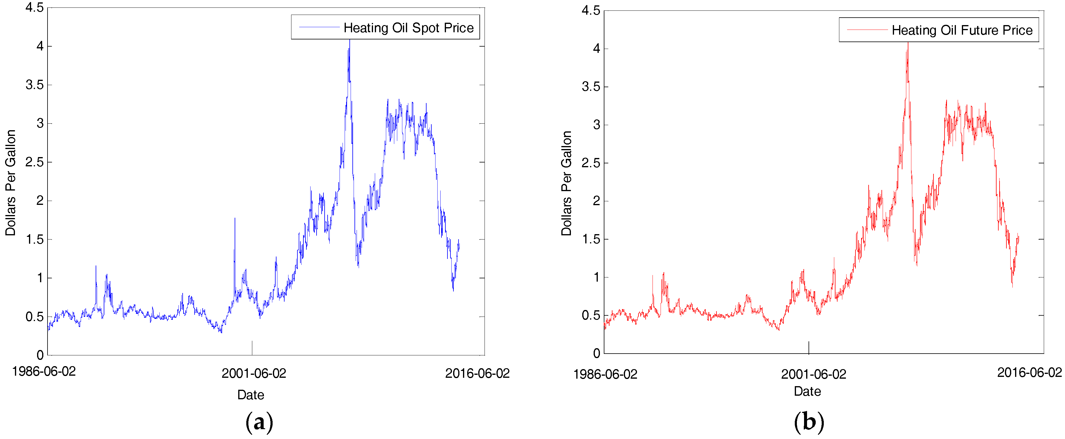
Figure 2.
(a) Probability evolution images of five fluctuation states of heating oil spot prices; (b) Evolution images of and ; (c) Evolutionary images of rise and decline in the volatile fluctuation period.
Figure 2.
(a) Probability evolution images of five fluctuation states of heating oil spot prices; (b) Evolution images of and ; (c) Evolutionary images of rise and decline in the volatile fluctuation period.
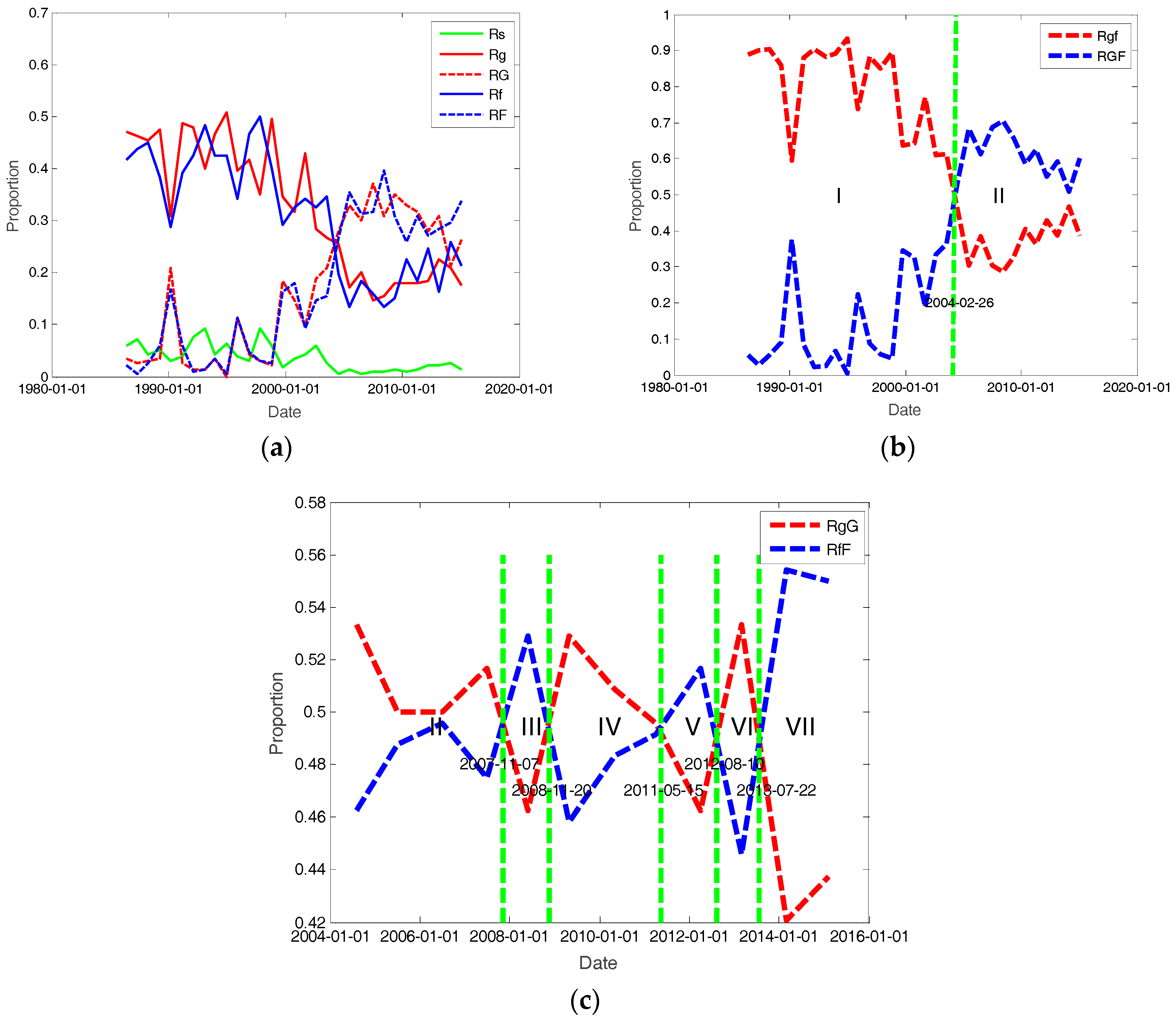
Figure 3.
(a) Probability evolution images of five fluctuation states of heating oil futures prices; (b) Evolution images of and ; (c) Evolutionary images of rise and decline in the volatile fluctuation period.
Figure 3.
(a) Probability evolution images of five fluctuation states of heating oil futures prices; (b) Evolution images of and ; (c) Evolutionary images of rise and decline in the volatile fluctuation period.

Figure 4.
The spot price fluctuation network of heating oil (a) and seven corresponding networks of different periods (b–h).
Figure 4.
The spot price fluctuation network of heating oil (a) and seven corresponding networks of different periods (b–h).
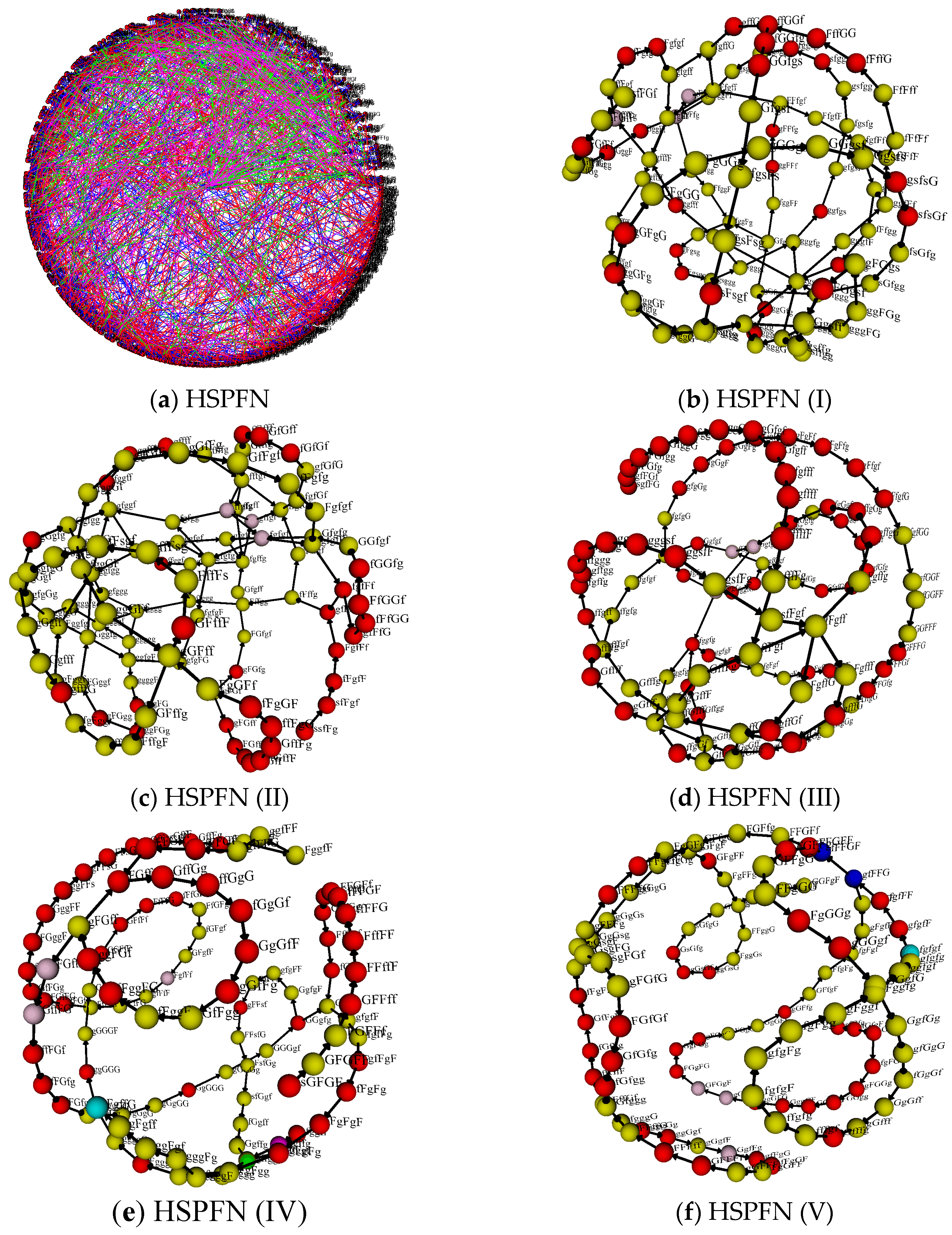

Figure 5.
The futures price fluctuation network of heating oil (a) and six corresponding networks of different periods (b–g).
Figure 5.
The futures price fluctuation network of heating oil (a) and six corresponding networks of different periods (b–g).


Figure 6.
(a) The cumulative time intervals of new nodes in HSPFN and HFPFN; (b) The cumulative time intervals of new nodes in different periods of HSPFN and HFPFN.
Figure 6.
(a) The cumulative time intervals of new nodes in HSPFN and HFPFN; (b) The cumulative time intervals of new nodes in different periods of HSPFN and HFPFN.

Figure 7.
(a) The distance between any two nodes in HSPFN; (b) The distance between any two nodes in HFPFN; (c) The distance distribution of nodes in HSPFN; (d) The distance distribution of nodes in HFPFN.
Figure 7.
(a) The distance between any two nodes in HSPFN; (b) The distance between any two nodes in HFPFN; (c) The distance distribution of nodes in HSPFN; (d) The distance distribution of nodes in HFPFN.

Figure 8.
(a) The path length distribution between nodes in different periods of HSPFN; (b) The path length distribution between nodes in different periods of HFPFN.
Figure 8.
(a) The path length distribution between nodes in different periods of HSPFN; (b) The path length distribution between nodes in different periods of HFPFN.
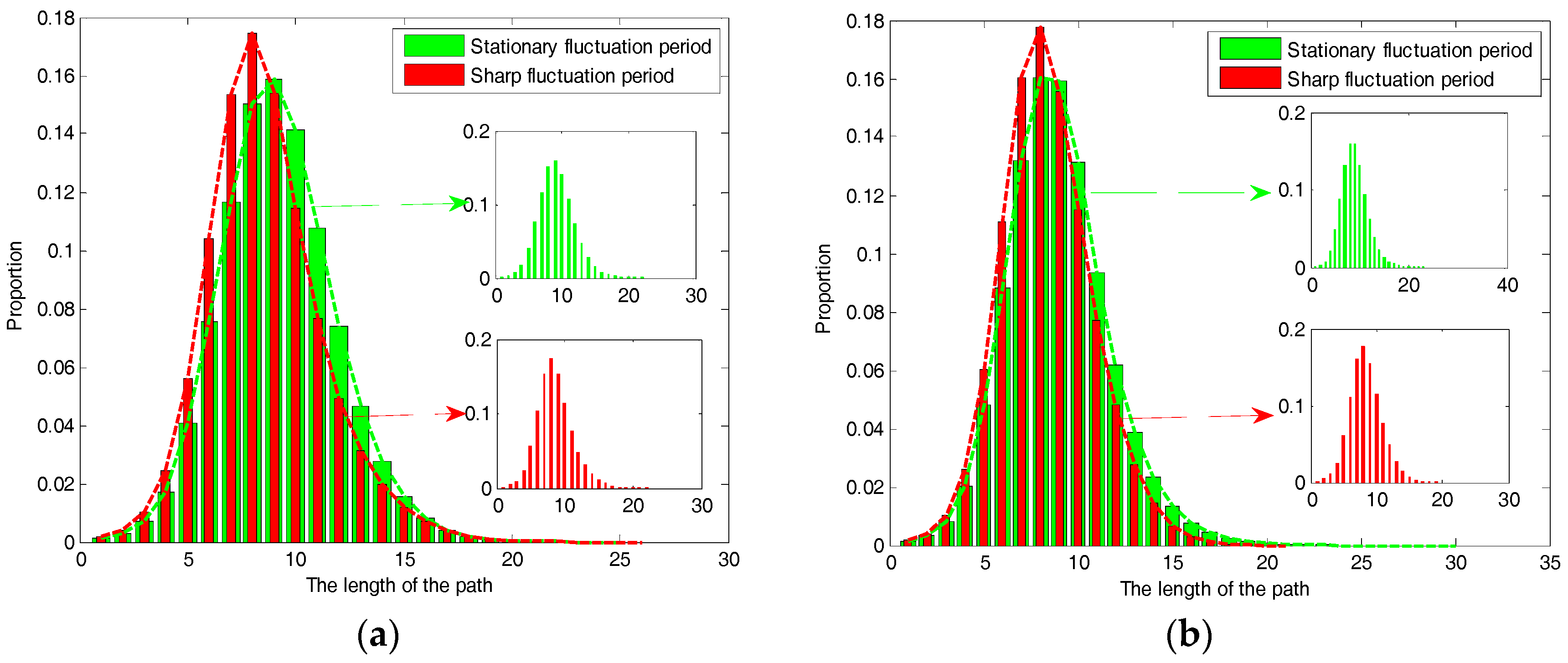
Figure 9.
(a) Strength and cumulative strength distribution of spot price nodes; (b) Strength and cumulative strength distribution of futures price nodes.
Figure 9.
(a) Strength and cumulative strength distribution of spot price nodes; (b) Strength and cumulative strength distribution of futures price nodes.

Figure 10.
(a) Occurrence time of important nodes in HSPFN; (b) Occurrence time of important nodes in HFPEN.
Figure 10.
(a) Occurrence time of important nodes in HSPFN; (b) Occurrence time of important nodes in HFPEN.
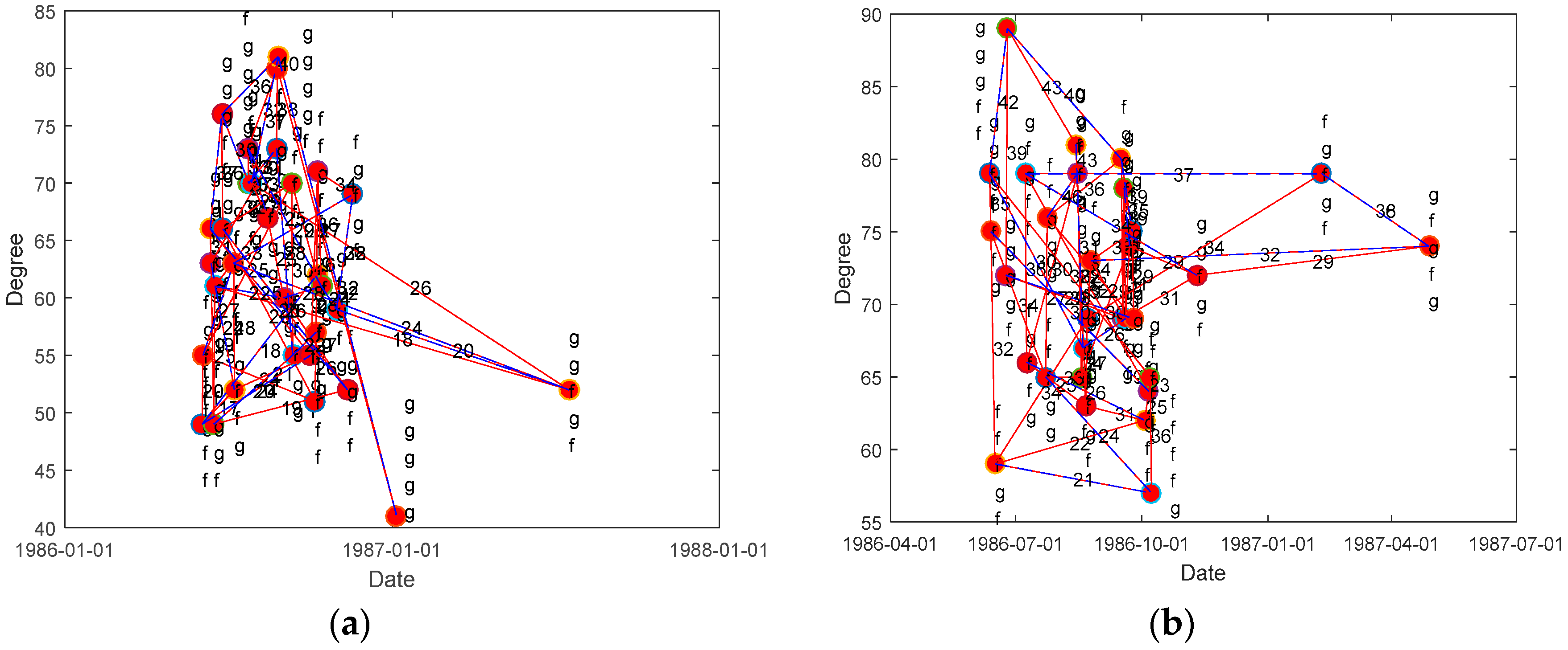
Figure 11.
(a) Important nodes and their links in HSPFN; (b) Important nodes and their links in HFPFN.
Figure 11.
(a) Important nodes and their links in HSPFN; (b) Important nodes and their links in HFPFN.

Figure 12.
(a) Double-logarithmic image of node strength in HSPFN; (b) Double-logarithmic image of node strength in HFPFN.
Figure 12.
(a) Double-logarithmic image of node strength in HSPFN; (b) Double-logarithmic image of node strength in HFPFN.
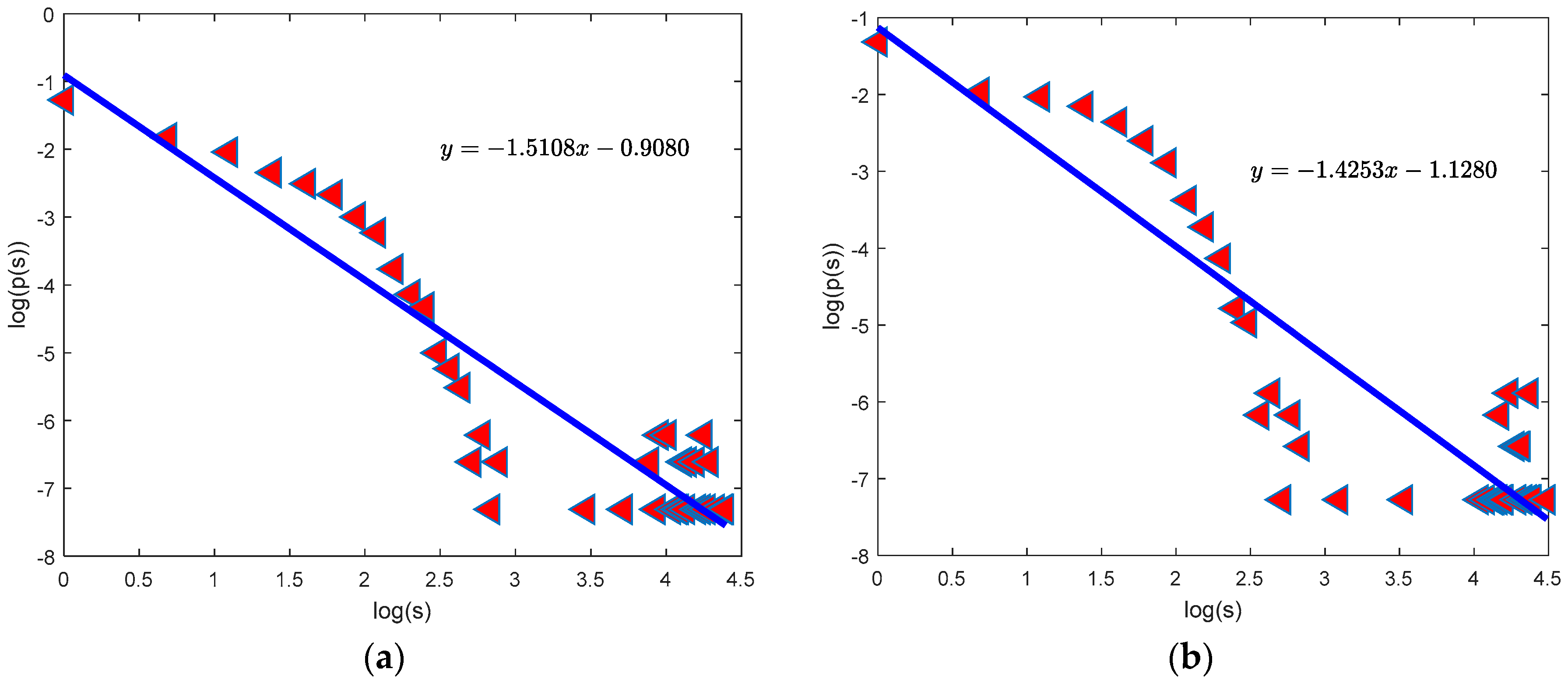
Figure 13.
(a) Double-logarithmic images of node strength in different periods of HSPFN; (b) Double-logarithmic images of node strength in different periods of HFPFN.
Figure 13.
(a) Double-logarithmic images of node strength in different periods of HSPFN; (b) Double-logarithmic images of node strength in different periods of HFPFN.
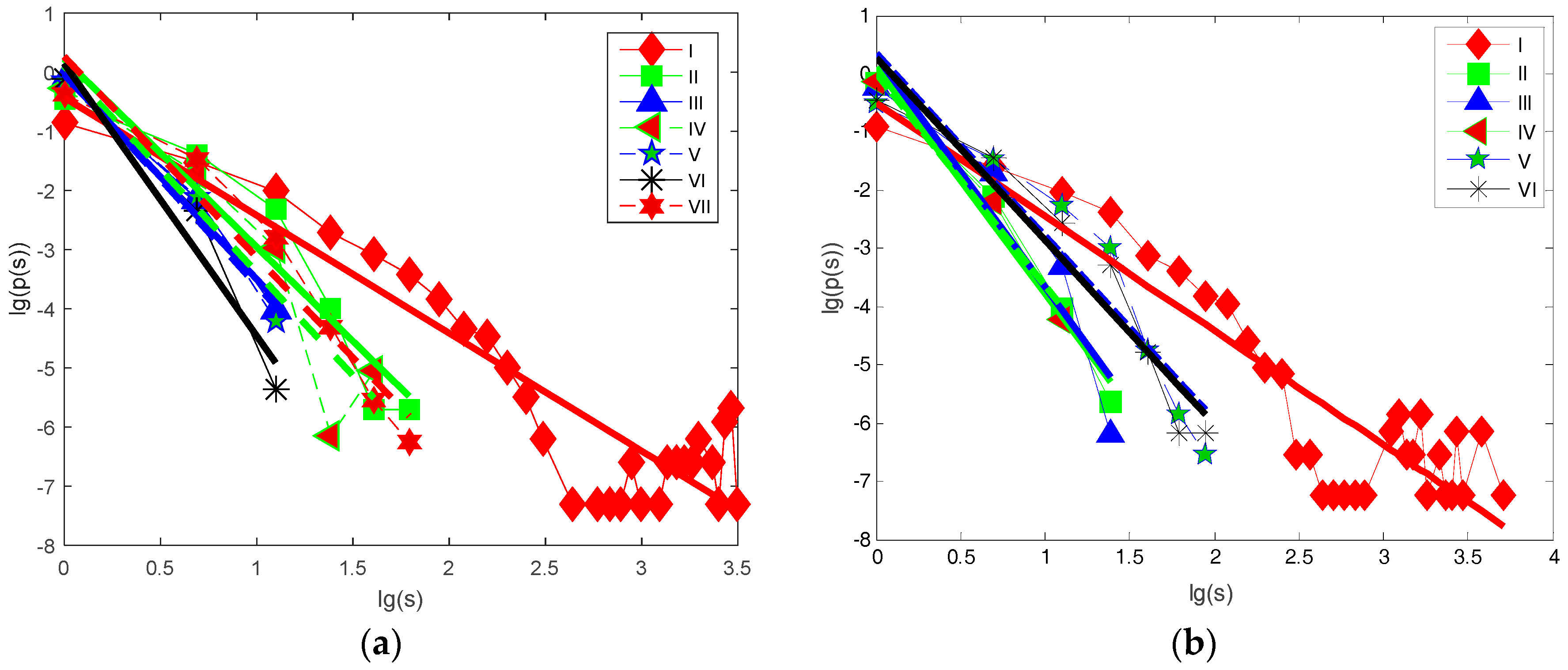
Figure 14.
Characteristics of the same nodes in HSPFN and HFPFN.

Figure 15.
(a) Statistics of the same nodes of HSPFN and HFPFN in stable fluctuation period; (b) Statistics of the same nodes of HSPFN and HFPFN in sharp fluctuation period.
Figure 15.
(a) Statistics of the same nodes of HSPFN and HFPFN in stable fluctuation period; (b) Statistics of the same nodes of HSPFN and HFPFN in sharp fluctuation period.

Figure 16.
(a) The evolution relationship with time between betweenness and strength of nodes in HSPFN; (b) The evolution relationship with time between betweenness and strength of nodes in HFPFN.
Figure 16.
(a) The evolution relationship with time between betweenness and strength of nodes in HSPFN; (b) The evolution relationship with time between betweenness and strength of nodes in HFPFN.

Figure 17.
(a)The evolution of node strength and betweenness during steady fluctuation period in HSPFN; (b) The evolution of node strength and betweenness during steady fluctuation period in HFPFN; (c) The evolution of node strength and betweenness during sharp fluctuation period in HSPFN; (d) The evolution of node strength and betweenness during sharp fluctuation period in HFPFN.

Figure 18.
(a) The clustering coefficient of HSPFN; (b) The clustering coefficient of HFPFN.

Figure 19.
(a) Clustering coefficients of HSPFN during the stable fluctuation period; (b) Clustering coefficients of HFPFN during the stable fluctuation period; (c) Clustering coefficients of HSPFN during the violent fluctuation period; (d) Clustering coefficients of HFPFN during the violent fluctuation period.

Figure 20.
(a) The nodes with larger strength or larger betweenness or larger clustering coefficient in HSPFN; (b) Time distributions of the first appearance of those nodes with larger strength or larger betweenness or larger clustering coefficient in HSPFN; (c) The nodes with larger strength or larger betweenness or larger clustering coefficient in HFPFN; (d) Time distributions of the first appearance of those nodes with larger strength or larger betweenness or larger clustering coefficient in HFPFN.
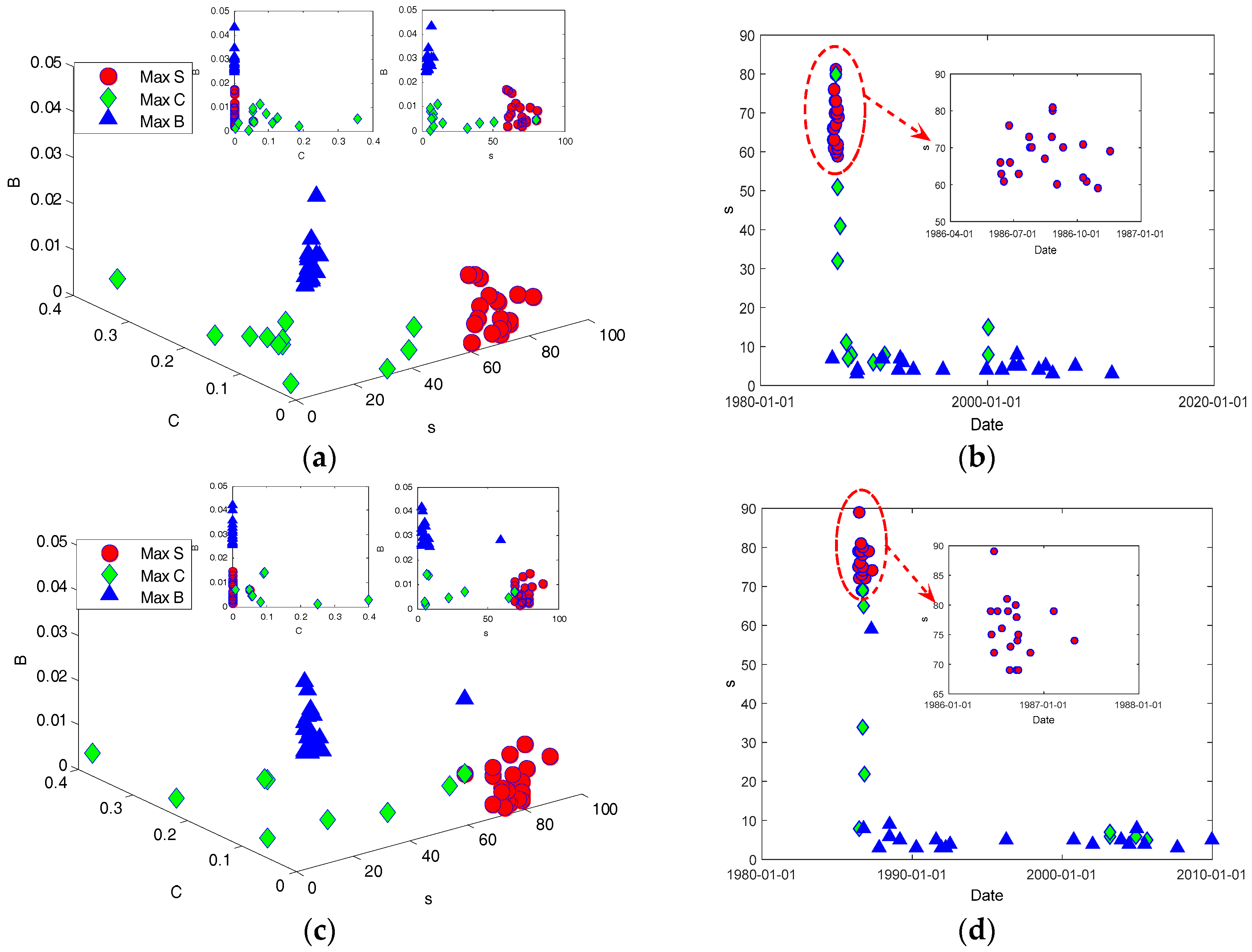

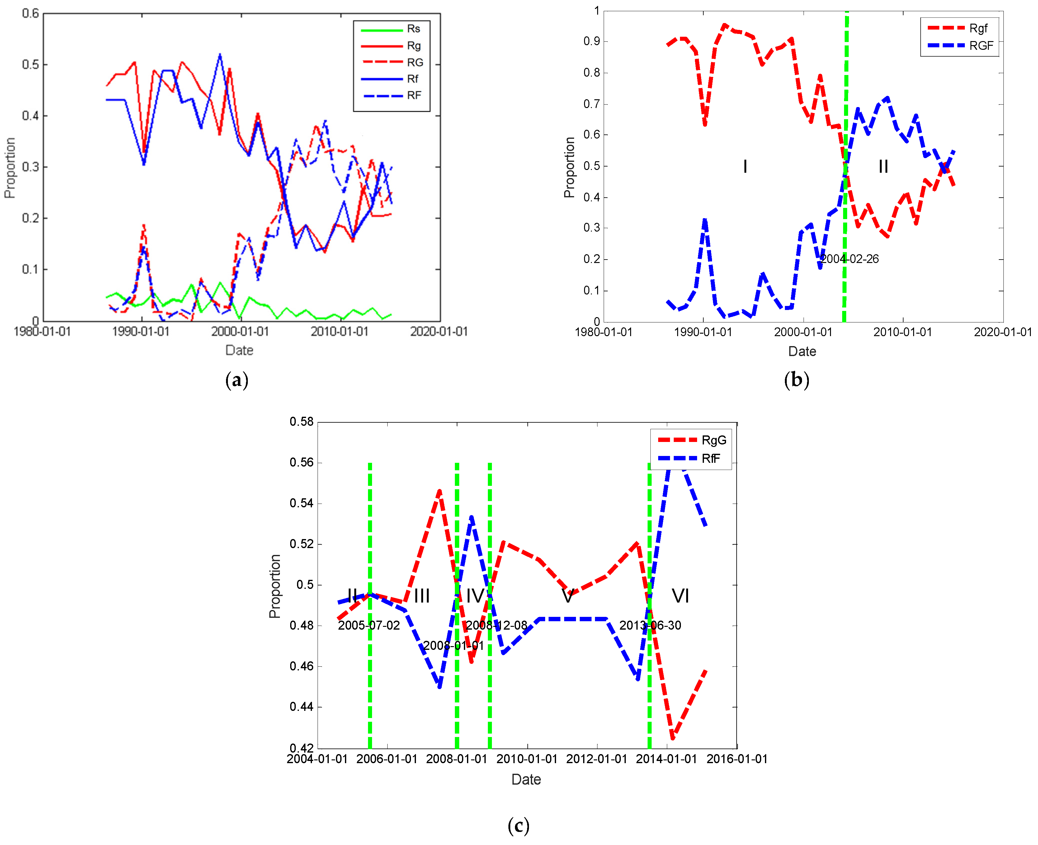
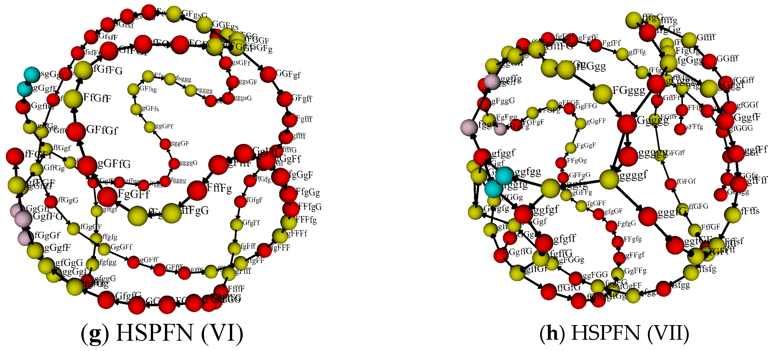
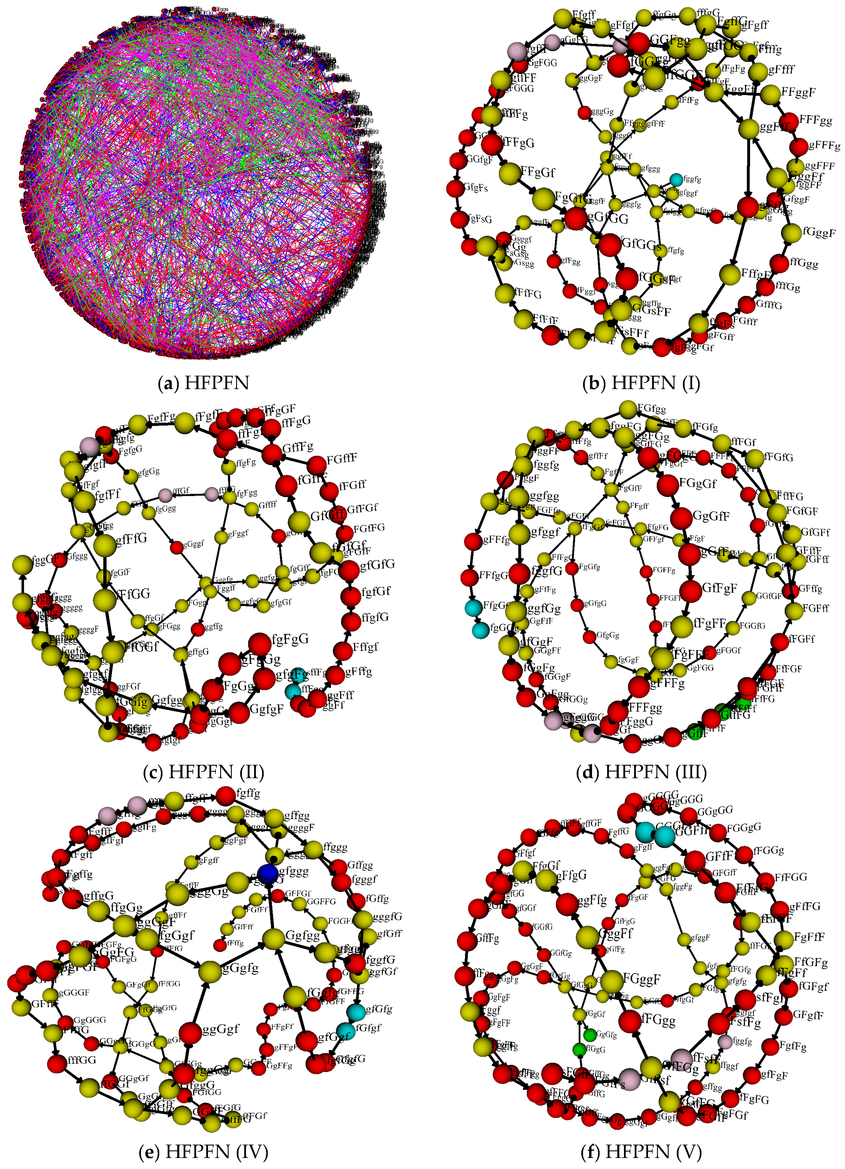
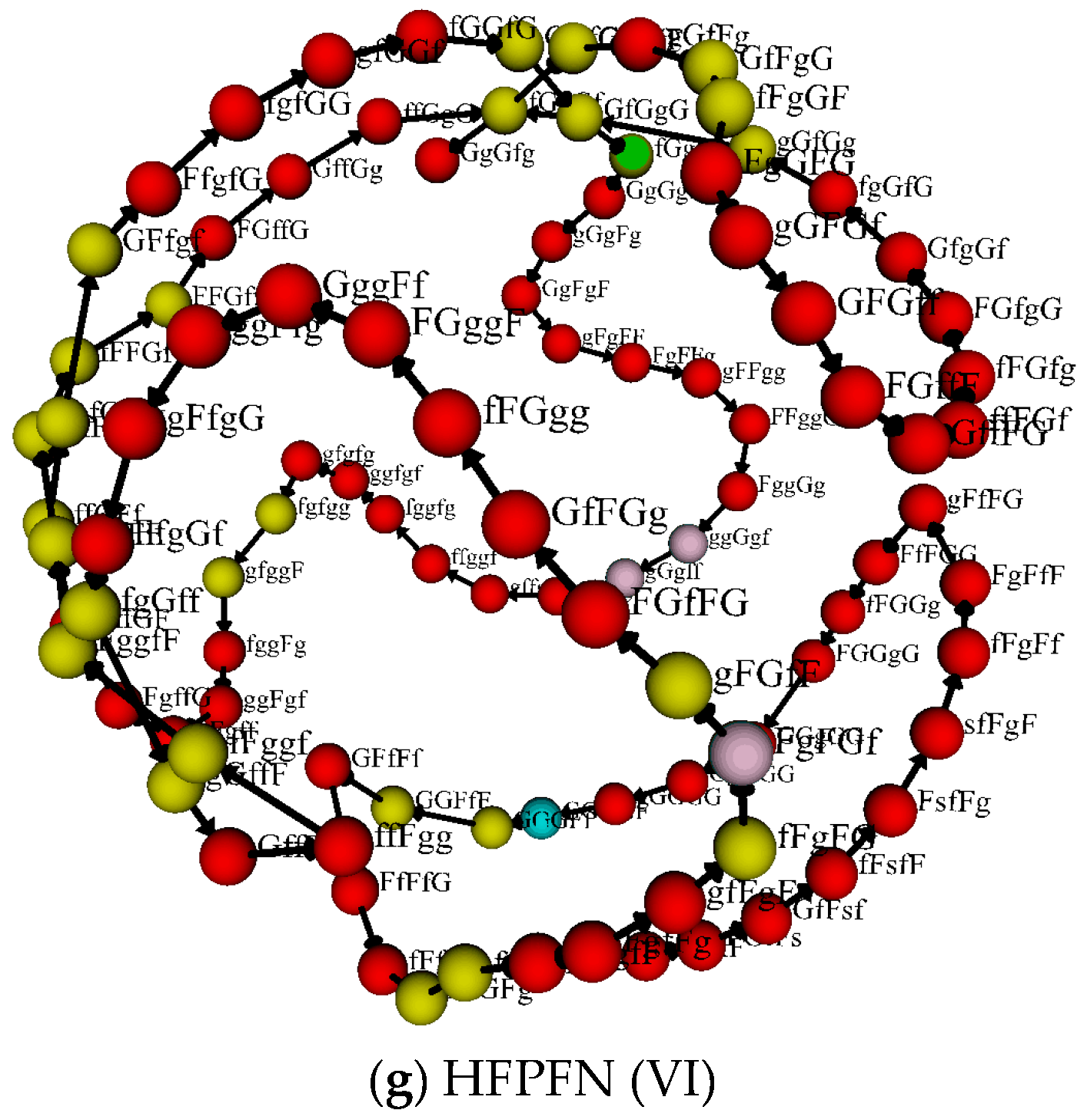
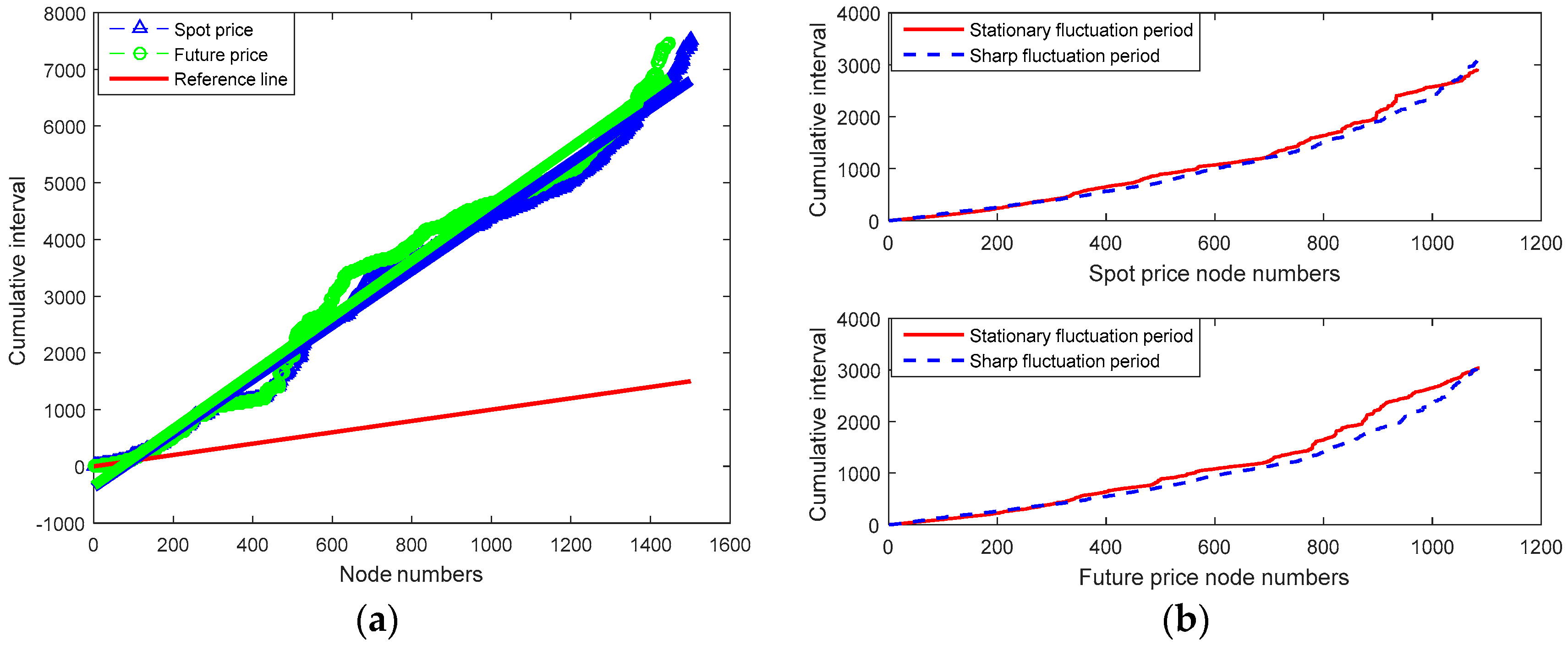
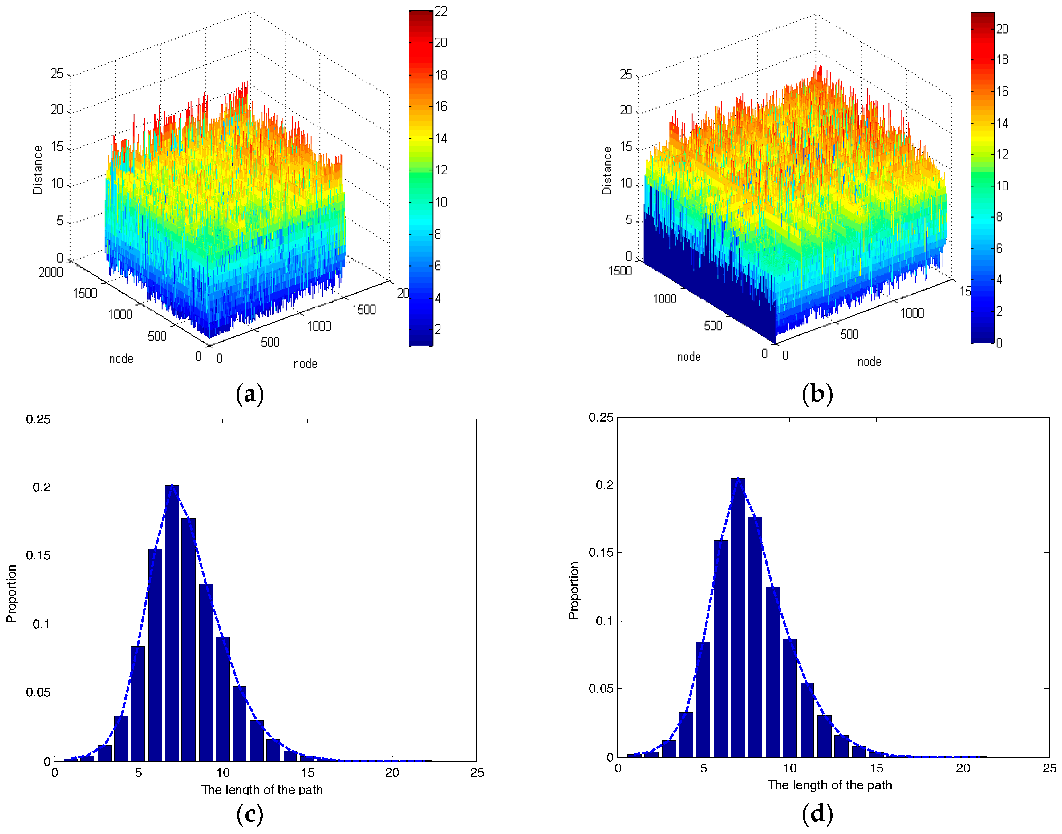
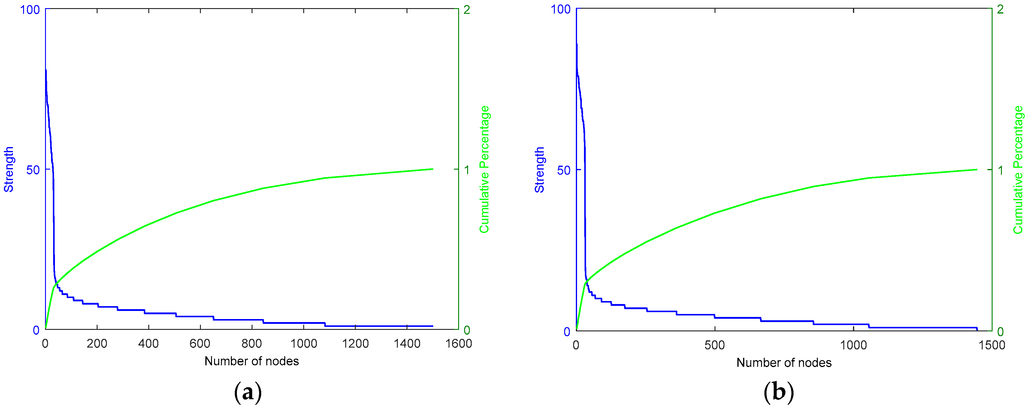
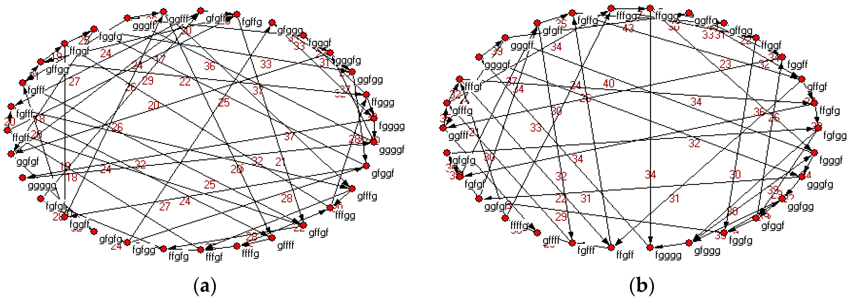
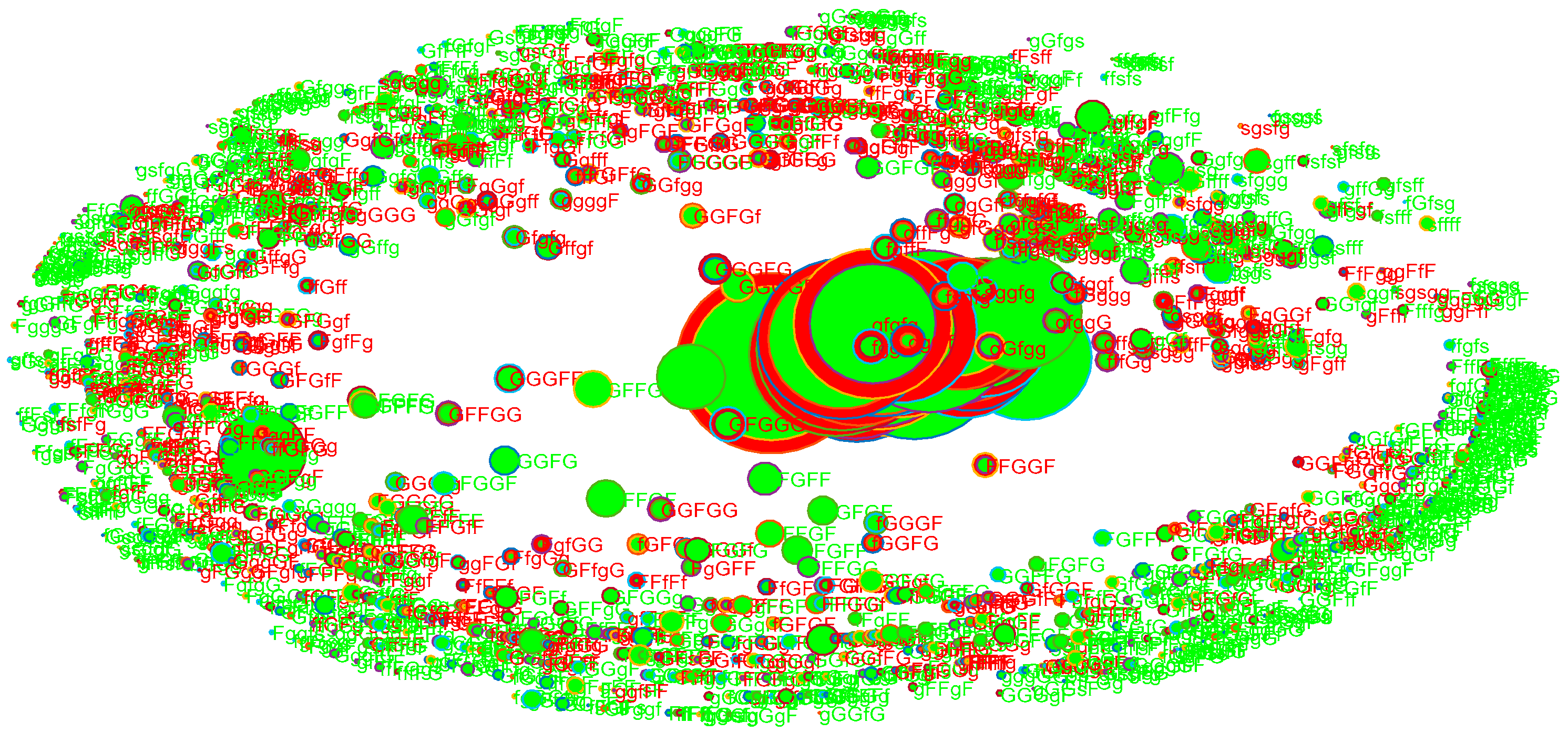
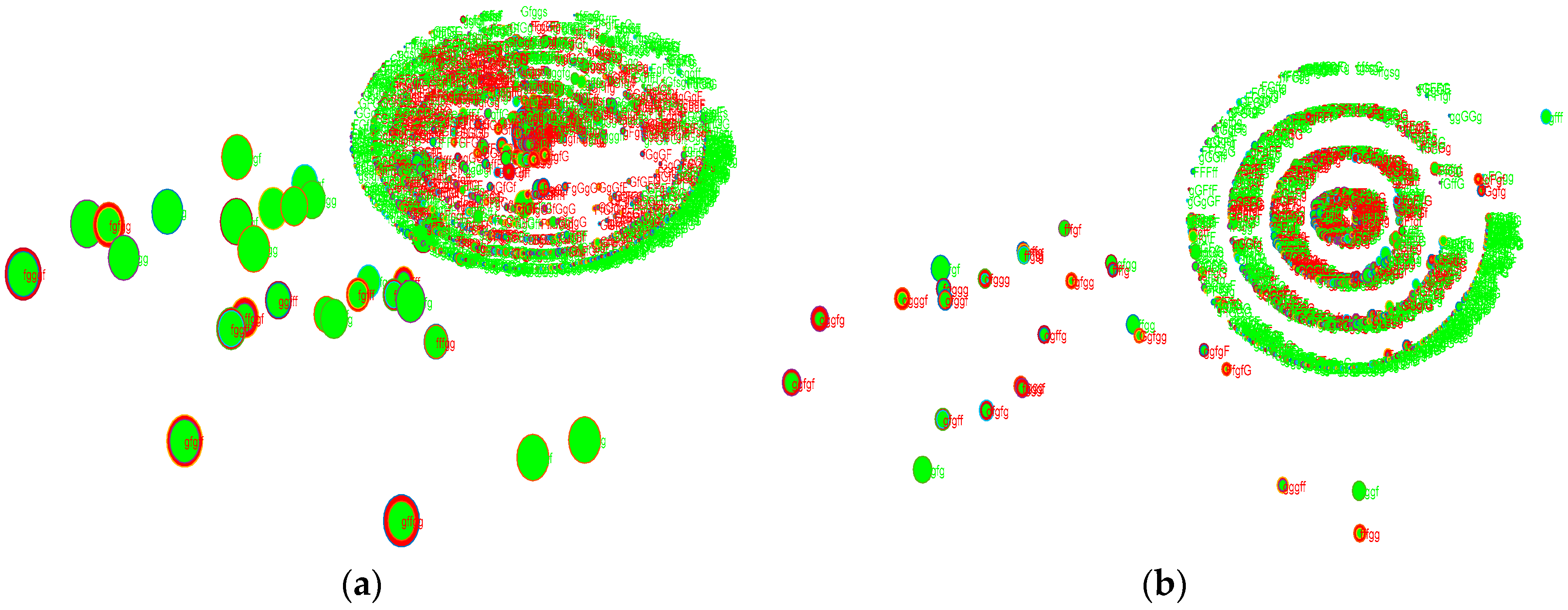
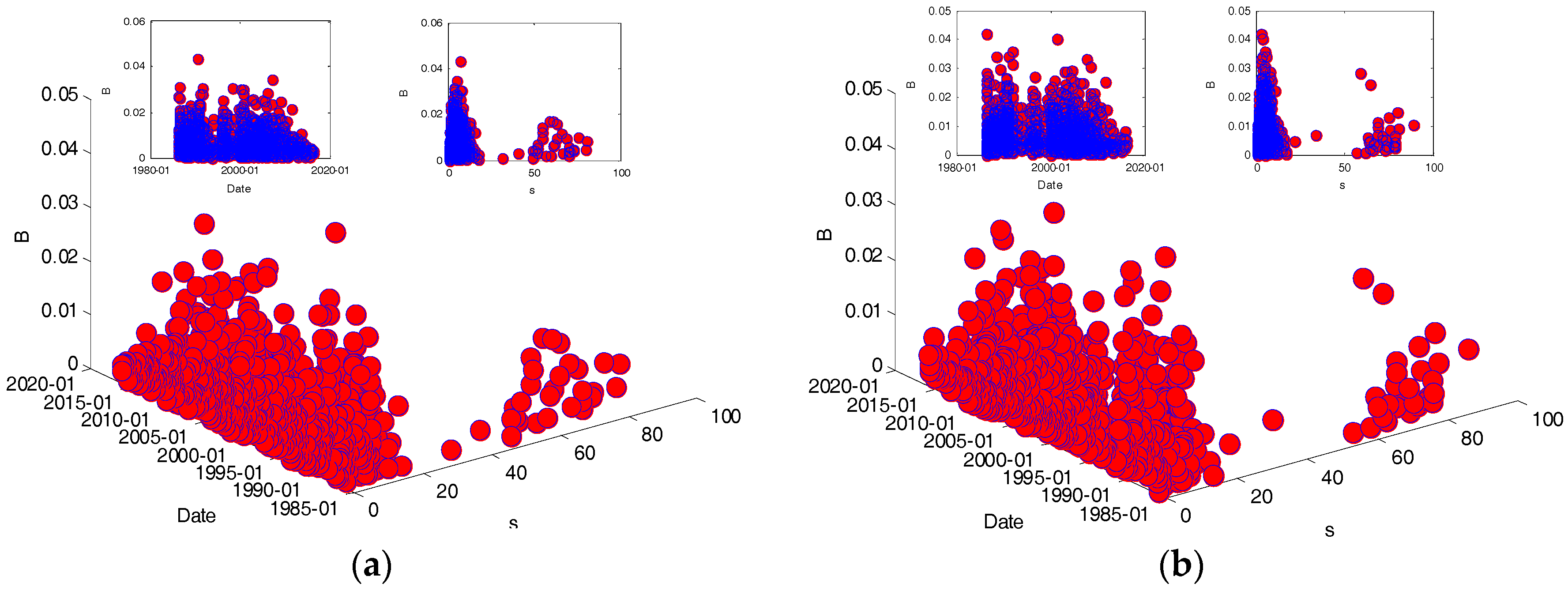
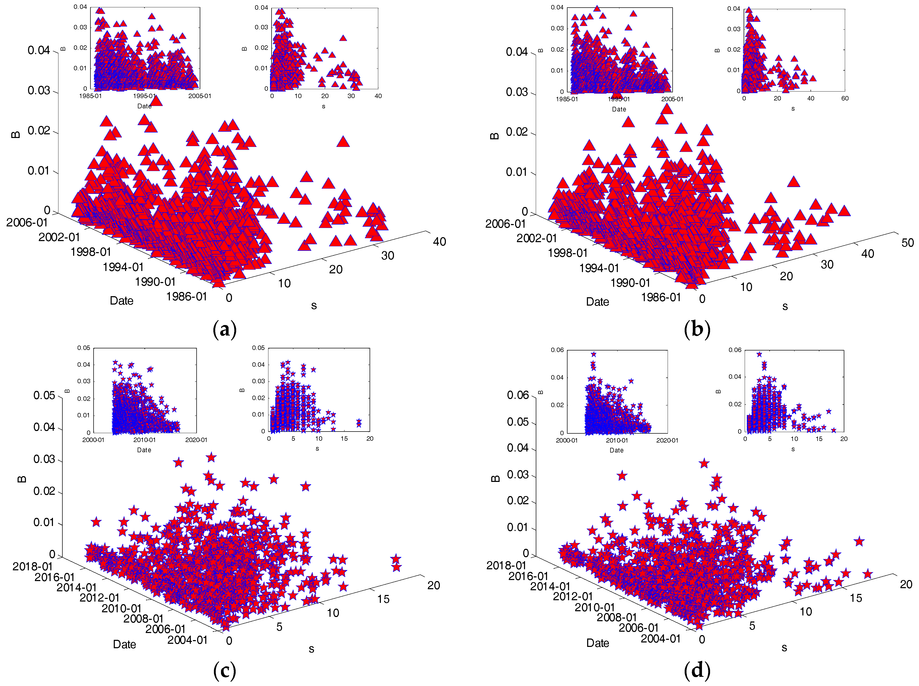
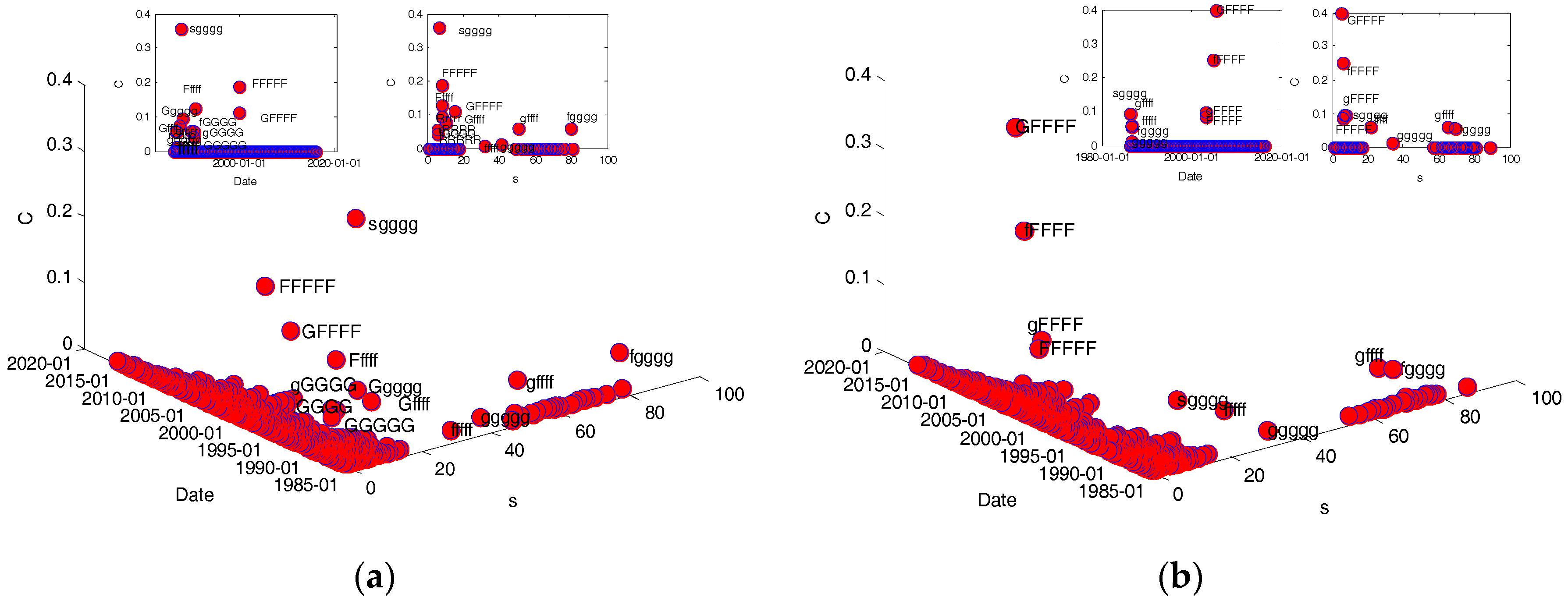
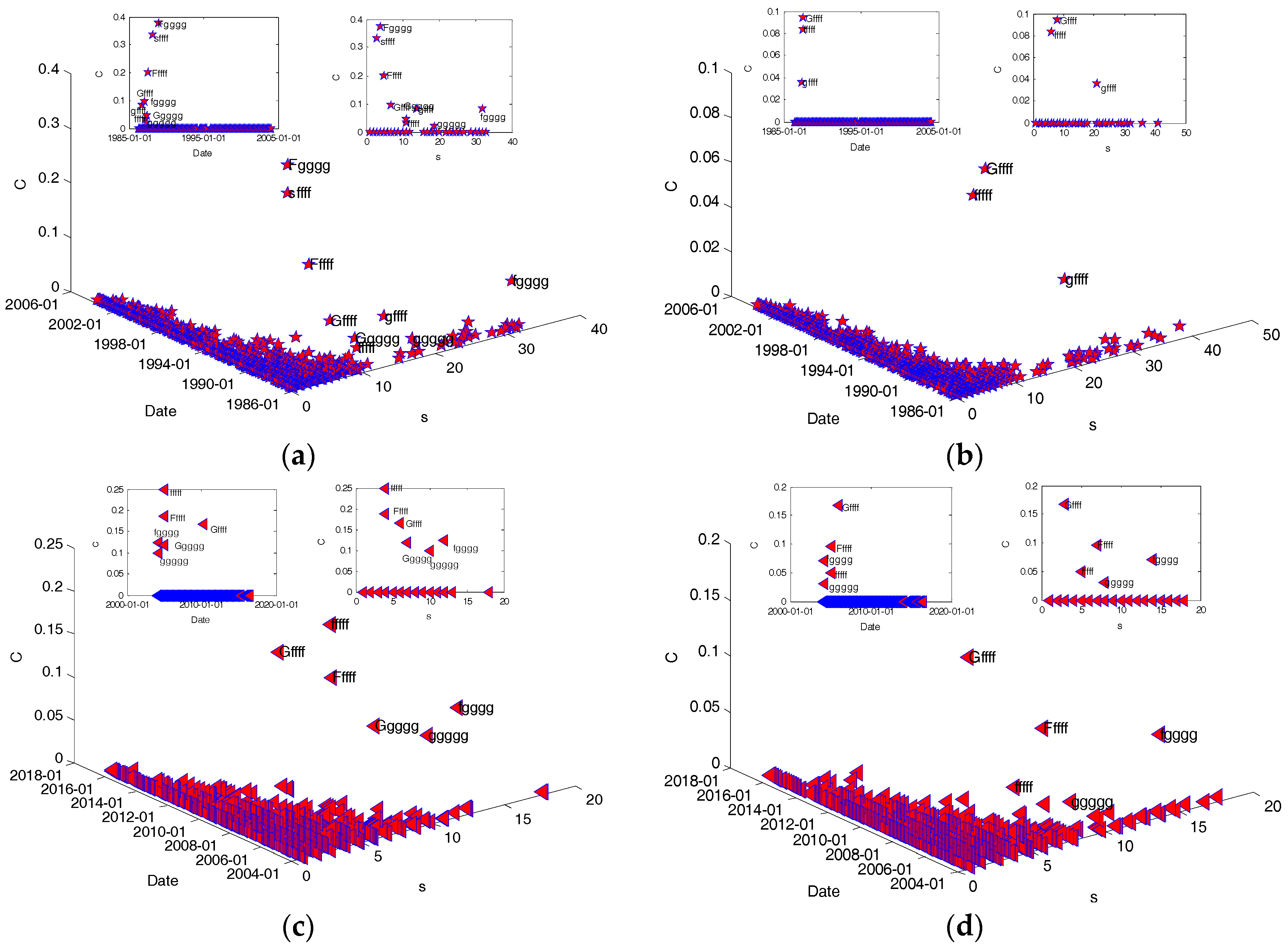
Table 1.
The fluctuation period division of heating oil spot price.
| Number | Periods of Time | Fluctuation State |
|---|---|---|
| I | 2 June 1986–26 February 2004 | Stable fluctuation period |
| II | 27 February 2004–7 November 2007 | Sharp rise period |
| III | 8 November 2007–20 November 2008 | Sharp decline period |
| IV | 21 November 2008–15 May 2011 | Sharp rise period |
| V | 16 May 2011–10 August 2012 | Sharp decline period |
| VI | 11 August 2012–22 July 2013 | Sharp rise period |
| VII | 23 July 2013–1 July 2016 | Sharp decline period |
Table 2.
The fluctuation period division of heating oil futures prices.
| Number | Periods of Time | Fluctuation State |
|---|---|---|
| I | 2 June 1986–26 February 2004 | Stable fluctuation period |
| II | 27 February 2004–2 July 2005 | Sharp decline period |
| III | 3 July 2005–1 January 2008 | Sharp rise period |
| IV | 2 January 2008–8 December 2008 | Sharp decline period |
| V | 9 December 2008–30 June 2013 | Sharp rise period |
| VI | 1 July 2013–1 July 2016 | Sharp decline period |
Table 3.
The construction process of the directional weighted for heating oil spot price fluctuations.
Table 3.
The construction process of the directional weighted for heating oil spot price fluctuations.
| Date | Mode | |||
|---|---|---|---|---|
 | ||||
Table 4.
The relevant statistics of important nodes in HSPFN and HFPFN.
| Number of Nodes (%) | Number of Important Nodes (Strength ) | Proportion of Important Nodes (%) | Proportion of the Sum of Strength of Important Nodes (%) | Average Contribution Ratio between Important Nodes (%) | |
|---|---|---|---|---|---|
| HSPFN | 1501 | 31 | 2.07% | 28.6% | 85.74% |
| HFPFN | 1446 | 30 | 2.07% | 28.6% | 87.27% |
Table 5.
Fitting parameters of node strength distribution for HSPFN and HFPFN in different periods.
| Periods | |||
|---|---|---|---|
| HSPFN | I | 1.9920 | 0.8425 |
| II | 3.1818 | 0.8999 | |
| III | 3.4599 | 0.9831 | |
| IV | 3.4878 | 0.8566 | |
| V | 3.5974 | 0.9729 | |
| VI | 4.6064 | 0.9469 | |
| VII | 3.3918 | 0.9410 | |
| HFPFN | I | 1.9576 | 0.8281 |
| II | 3.8976 | 0.9740 | |
| III | 3.9658 | 0.8760 | |
| IV | 3.6289 | 0.9778 | |
| V | 3.1332 | 0.8865 | |
| VI | 3.1488 | 0.9171 |
© 2017 by the authors. Licensee MDPI, Basel, Switzerland. This article is an open access article distributed under the terms and conditions of the Creative Commons Attribution (CC BY) license (http://creativecommons.org/licenses/by/4.0/).
Share and Cite
MDPI and ACS Style
Chen, H.; Tian, L.; Wang, M.; Zhen, Z. Analysis of the Dynamic Evolutionary Behavior of American Heating Oil Spot and Futures Price Fluctuation Networks. Sustainability 2017, 9, 574. https://doi.org/10.3390/su9040574
AMA Style
Chen H, Tian L, Wang M, Zhen Z. Analysis of the Dynamic Evolutionary Behavior of American Heating Oil Spot and Futures Price Fluctuation Networks. Sustainability. 2017; 9(4):574. https://doi.org/10.3390/su9040574
Chicago/Turabian StyleChen, Huan, Lixin Tian, Minggang Wang, and Zaili Zhen. 2017. "Analysis of the Dynamic Evolutionary Behavior of American Heating Oil Spot and Futures Price Fluctuation Networks" Sustainability 9, no. 4: 574. https://doi.org/10.3390/su9040574
Note that from the first issue of 2016, this journal uses article numbers instead of page numbers. See further details here.