Article

Research on the Coupling Coordination of a Sea–Land System Based on an Integrated Approach and New Evaluation Index System: A Case Study in Hainan Province, China

College of Management and Economics, Tianjin University, No. 92 Weijin Road, Tianjin 300072, China
*
Author to whom correspondence should be addressed.
Sustainability 2017, 9(5), 859; https://doi.org/10.3390/su9050859
Submission received: 24 February 2017 / Revised: 29 April 2017 / Accepted: 16 May 2017 / Published: 19 May 2017

Abstract

:
Based on the concept of sea–land coordination and the statistical data of Hainan Province from 1999 to 2013, we establish a new evaluation index system included four aspects—economic development, social progress, environmental protection and resource efficiency—and use the integrated approach (such as the combination weight method, the coupling coordination degree model, the scissors difference model and the dynamic coupling coordination degree model) to measure the coupling coordination degree of a sea–land system. The results show that: (1) the overall development level of sea system and land system are gradually improved; (2) the coupling coordination degree of sea–land system is gradually from moderately uncoordinated to well coordinated, and the comprehensive evaluation value of sea system has a greater effect on the coupling coordination degree D than that of land system; (3) the scissors difference between sea system and land system is gradually increasing; (4) the dynamic coupling coordination degree of the sea–land system which favors a parabolic shape is basically in the break-in development stage; (5) in the process of sea–land system coordination, the influencing factors of economic development, the social progress and resource efficiency should be given priority and, at the same time, strengthen the environmental protection efforts and awareness to promote the role of environmental protection in the sea–land coordination.

1. Introduction

The marine economy is developing rapidly in the 21st century. Since the beginning of the new century, in order to alleviate the energy shortage, resource shortage, ecological deterioration, and other issues, countries around the world have developed new national marine strategies, strategically laid out from land to sea, which results in fierce competition between marine economies [1]. However, with the rapid development of marine economies, the conflicts and contradictions between sea system and land system are becoming more and more prominent in terms of resources, environment, production elements, and space for development, which seriously restricts the sustainable development of sea system and land system. In addition, the effect of the marine economy in promoting the national economy is more and more limited [2]. Therefore, in order to solve the contradictions between sea system and land system and achieve sea–land system coordination, China has put forward the “The Five Plans as a Whole” principles of economic development [3] and future development goals of “adhering to sea–land coordination, formulating and implementing the marine development strategy, improving the capabilities of developing, controlling, and integrated marine management [4]”, making sea–land coordination a national development strategy. Thus, it is of important theoretical and practical significance to strengthen the research on sea–land coordination in coastal areas.
Zhang et al. [5] proposed the concept of “sea–land coordination” firstly. He thought that the concept of sea–land coordination was that in regional social development, the sea system and land system are two important subsystems that affect the development of the entire regional system, so the government needs to scientifically develop unified planning for oceans and land to achieve complementary advantages and coordination of interaction between the sea system and land system on the basis of taking into account the characteristics of the sea system and land system in terms of resources, environment, economy and social use, and using the links of logistics, energy flow, information flow, and so on between sea and land. The direct purpose of sea–land coordination is effectively using the advantages of the land system to support the breadth and depth of sea development, and then through the vitality of the sea system develop a greater room for improvement of land system. At the same time, the long-term purpose of the sea–land coordination is to achieve a reasonable allocation of sea resources and land resources to promote regional sustainable development.
A conceptual rendering of sea–land co-ordination is shown in Figure 1. The interaction mechanisms of sea system and land system are shown in Figure 2. The development levels of the sea system and land system are not the same in the regional development system, and the overall structure is a pyramid. Although the size of the sea system is small, as a pioneer in regional development, it is located at the top of the pyramid, while the scale of the land system which is located in the lower end of the pyramid is relatively large, and provides basic support for marine development. While giving full play to the guiding role of policy planning and expanding the support of the land system to the sea system, the sea system can rely on land-based infrastructure to expand its own scale. When the interaction between the sea system and the land system is so sufficient that the scale of the sea system is maximized, the radiation degree of the sea system to the land system also increases. This will create a broader space for the progress of the land system. If the land system continues to develop using these spaces, it will further provide greater support for the sea system. At this point, a virtuous circle is formed: the scale of the region is expanding and achieving the goal of coordinated and sustainable development.
There is not a concept of sea–land coordination in western countries, where the studies related to sea–land coordination are called integrated coastal zone management (ICZM) [6,7]. ICZM refers to an ongoing and dynamic process of formulating policy and management strategies to solve conflicts in the use of coastal resources and control the environmental impact of human activities on coastal areas. It mainly considers the ecological, economic, and social fields, and uses an integrated approach to plan and manage human activities in the marine and coastal zone [8]. Comparing the concepts of sea–land coordination and ICZM, we summarize the similarities and differences between them, and then summarize the advantages and disadvantages of developing sea–land coordination and ICZM (as shown in Table 1).
The similarities:
(1)
Comprehensive strategic objective. The ultimate goals of both approaches are to achieve the sustainable development of marine and coastal zones on the basis of a comprehensive consideration of the economic, environmental, social, and environmental needs.
(2)
Similarity of scope. They are both suitable for resource management of land and sea and the design of management mechanisms.
(3)
Diversification of means. They both emphasize the management of marine and coastal zones through policies, laws, regional planning, science and technology, education, training, and other means.
The differences:
(1)
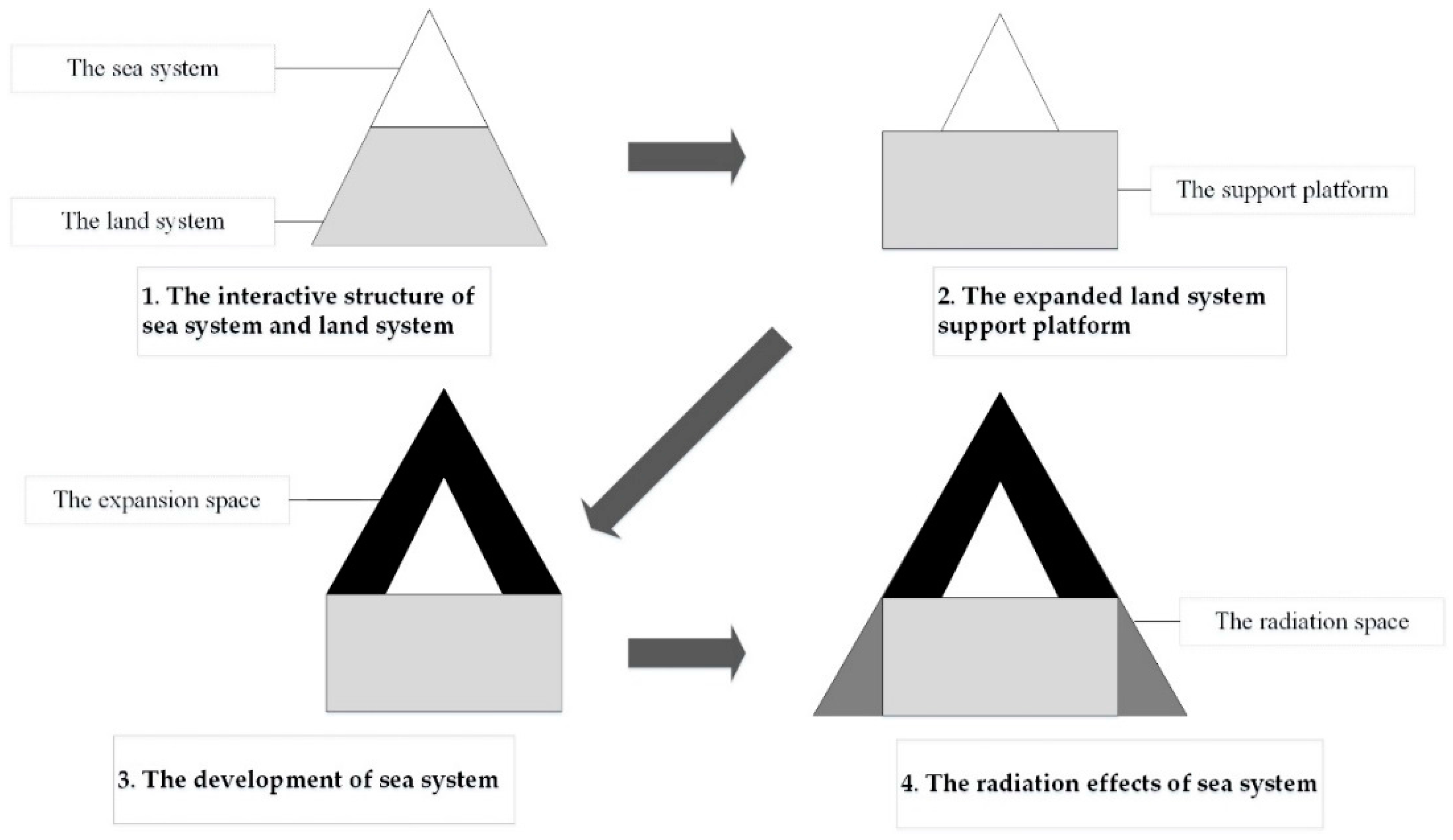
Focus. Sea–land coordination focuses on the characteristics of the marine system and the land system, and stresses the achievement of complementary advantages between the sea system and land system, two economic systems, through policy guidance and industry links. ICZM Manages and plans the development of coastal zones mainly based on natural, environmental, and social factors. It is more concerned about the ecological and environmental problems of the coastal zone, but it is less concerned about the development of the marine economy and coordination between the sea industry and land industry.
(2)
Viewing angle. Sea–land coordination solves the contradictions between sea system and land system from the perspective of the whole region. ICZM protects the environment and ecology of the coastal zone from the local perspective of the coastal zone.
(3)
Level. Sea–land coordination is a national strategy for the development of the sea economy and the land economy in China, and is a guiding ideology for planning and developing the marine and coastal economies. ICZM is a specific implementation process.
(4)
Scope of implementation. The spatial scope of sea–land coordination can not only cover marine and land areas, but also extend to international areas closely related to our interests. The spatial scope of the ICZM is a narrow strip.
At present, the research of Chinese scholars on sea–land coordination can be divided into two aspects: qualitative research and quantitative research. Qualitative research focuses on the connotations of “sea–land coordination” [9], the effects on the development of the marine economy [10], the problems facing it, the feasibility of implementation, and so on [11]. In the quantitative research, Yang et al. [12] used the Criteria Importance through Inter-criteria Correlation (CRITIC) and Analytic Hierarchy Process (AHP) methods to measure sea–land coordination in the Bohai Sea area from the perspectives of the industry, society, ecology and so on. Sun et al. [13] used the capacity structure model and AHP method to measure sea–land coordination from the perspectives of resources, industry, technology, and environment. Liang et al. [14] used the entropy weight method and coupling coordination degree model to evaluate the coupling degree of the sea–land system in Guangdong, China from the perspectives of economy, society, input, and sustainable development. Zhao et al. [15] used the entropy weight and coupling coordination degree model to measure sea–land coordination in China from the perspectives of environment, management, performance, structure, and technology.
The research areas of sea–land coordination have been mainly concentrated on the Bohai Sea, the Yellow Sea and the East Sea of China. Fan et al. [16] analyzed the differences of basic conditions of sea–land coordination in different areas of Liaoning using the statistical data of Liaoning Province as the study sample. Jiang et al. [17] analyzed how to promote the development of the Shandong Peninsula Blue Economic Zone from three levels: the macro view, middle view and micro view. Through the analysis of the correlation between the marine industry and the land industry in Jiangsu Province, Chang et al. [18] put forward effective measures to promote the development of marine and land industry. Hainan has long been China’s major marine economic province, so there is a great deal of research into its marine economy. Through the analysis of the marine industry in Hainan Province, Ye et al. [19] identified the leading and dominant marine industries of Hainan, and proposed countermeasures of marine industry structure optimization and upgrading. Wu et al. [20] investigated the present situation of marine economic development and marine environmental protection in Hainan Province, pointed out the problems existing in protection of the ecological environment, and put forward some suggestions. Zhang et al. [21] constructed an ecological risk assessment model to analyze the main risks of tourism in Hainan, and provided some guidance for the rapid development of tourism in Hainan.
In summary, there is still a very broad space for research on sea–land coordination at home and abroad. Firstly, there is the evaluation index system. From the concept of the sea–land coordination, we can know that the four functions of sea–land coordination include economy, society, environment, and resources, and that these should be fully considered in the evaluation process of sea–land coordination, but in the existing literature, the evaluation index system of sea–land coordination has not yet considered these four aspects. Secondly, research methods. At present, in the quantitative research of sea–land coordination, the methods of determining the weight of the indexes are mostly single. What is more, the research method into the coupling coordination degree of the sea system and the land system is limited to the coupling coordination degree model, while the scissors difference model and the dynamic coupling coordination degree model have not been used. Finally, research areas need to be expanded. In the existing literature, the research on sea–land coordination is mainly concentrated on the Bohai Sea, the Yellow Sea and the East Sea of China. There is little research on sea–land coordination in the South China Sea. However, in recent years, with the increasing concern of the Chinese government on the South China Sea issue as a base for the development of the South China Sea, it is necessary for Hainan to implement the policy of sea–land coordination.
Therefore, in this paper, firstly, we take Hainan Province as the research object, and construct a new evaluation index system of sea–land coordination including four aspects: economic development, social progress, environmental protection, and resource efficiency. Secondly, we use a chain of methods which includes the combination weight method, the coupling coordination degree model, the scissors difference model, and the dynamic coupling coordination degree model, to measure the sea–land coordination degree of Hainan. Finally, according to the conclusions, this paper puts forward relevant suggestions for the development of Hainan which have important practical significance for promoting the sustainable development of the sea–land system in Hainan Province.

2. Materials and Methods

2.1. Materials

2.1.1. Study Area

Hainan Province (Qiong for short) lies between 108°37′ E to 111°05′ E and 18°10′ N to 20°10′ N, and is in the southern tip of China [22]. The coastline length of Hainan is 1823 km, and the land area and the sea area are 35 thousand km2 and 2 million km2 respectively. The scope of its administrative region includes the Hainan, Xisha, Nansha, and Zhongsha Islands and it is located at the northern edge of the tropical zone, having a tropical monsoon climate. The Special Economic Zone of Hainan Province is the only provincial Special Economic Zone and Hainan Island is the second largest island in China outside of Taiwan Island. With rich marine and land resources as well as the country’s high attention, the economy, society, environment, and resources of Hainan Province have made great progress. In economic respects, Gross Domestic Product (GDP) rose from 47 billion CNY in 1999 to 314 billion CNY in 2013, and the Gross Marine Product (GMP) rose from 5 billion CNY in 1999 to 88 billion CNY in 2013. In social respects, the living standard of urban and rural residents continues to improve. The per capita disposable income of urban households rose from 5338 CNY in 1999 to 22,929 CNY in 2013, and education and health are achieving new development. The financial expenditure on education, health, and science rose from 130 million CNY in 1999 to 279.9 (100 million CNY) in 2013. The carrying capacity of the ports has also been gradually rising. The number of berths for port production increased from 46 in 1999 to 76 in 2013. The scale of marine science and technology practitioners has been expanding, and the number of people rose from 30 in 1999 to 212 in 2013. In environmental respects, the capacity of environmental governance has increased, and the urban air quality is generally fine. The investment into pollution control increased from 24,030 thousand CNY in 1999 to 16,344 million in 2013. The per capita marine nature reserve area increased from 1 m2 in 1999 to 27.5 m2 in 2013. In 2013, the proportion of good urban air quality is 99%. In terms of resources, the utilization efficiency of resources continues to increase. The regional economic density increased from 14,100 million/km in 1999 to 89,000 million/km in 2013; the coastline economic density increased from 31 million/km in 1999 to 173 million/km in 2013.
However, in recent years, due to the excessive development of the marine economy, the competition for production elements between sea system and land system is more and more intense. Due to depletion, development, severe resource waste, and the vulnerability of the ecological environment, competition between the sea system and the land system is very prominent. All those have seriously hindered the sustained, healthy, and rapid development of Hainan. Therefore, it is imperative to coordinate the development of the sea–land system.

2.1.2. The Indexes System

Since the 21st century, the relationship between sea and land has become more and more complex [23]. On the one hand, spatial dependence and the complementation of production factors make coordination and sustainable development of sea and land possible. On the other hand, more intense competition for development space and production elements makes coordination and sustainable development of sea system and land system difficult. Thus, the system that consists of the sea system and the land system can be defined as a coupling system. Obviously, the coupling coordination degree is used to represent the degree of interaction between the two systems [24]. To measure the relationship between the sea system and the land system, we determined the preliminary indexes framework by searching the literature [25,26,27], and then in accordance with the actual situation in Hainan Province, we constructed a final evaluation indexes system based on the principles of appropriateness, comparability, and accessibility. The indexes system of the sea system and land system contains 4 subsystems (economic development, social progress, environmental protection, and resource efficiency) and 16 basic grade indicators respectively. The final evaluation indexes system is displayed in Table 2.
The u A H P denotes the weight coefficient of the AHP method, u I E W represents the weight coefficient of the information entropy weight (IEW) method, and u C W denotes the weight coefficient of the combination weight of game theory (CW).

2.2. Methods

2.2.1. Data Pre-Processing

The relative sea statistic data (1999–2013) were acquired from the China Marine Statistical Yearbook (National Bureau of Statistics of the People’s Republic of China, 1999–2013), and the relative land statistic data (1999–2013) were acquired from the Statistical Yearbook of Hainan Province (Hainan Provincial Bureau of Statistics, 1999–2013). For this paper, the temporal and spatial sequence data of Hainan Province from 1999 to 2013 were selected and the data are standardized as Equations (1) and (2) to exclude the influence of dimension, magnitude, and positive and negative orientation (as shown in Table A1 and Table A2 in Appendix A) [28,29].
Positive indicator:
X i j = ( X i j min { X j } ) / ( max { X j } min { X j } )
Negative indicator:
X i j = ( max { X j } X i j ) / ( max { X j } min { X j } )
where X i j denotes the value of indicator j in year i and max { X j } and min { X j } indicate the maximum and minimum values of indicator j for all years respectively. Thus, all of the indexes values are in the range of ( 0 , 1 ) .

2.2.2. Evaluation of the Statistical Data

To overcome the limits of the subjective evaluation method and the objective evaluation method, a combination weight method has been widely adopted in recent research [30]. To make the evaluation process more reasonable, we selected the AHP as a subjective weighting method and the IEW as an objective weighting method to determine the combination weight of each indicator based on game theory. The calculation process for AHP and IEW can be found in References [31,32,33,34].
The calculation process of combination weight based on game theory is as follows [35]:
Step (1): Obtain n weights according to n types of weighting methods, and then construct a basic weight vector set U | = { u 1 , u 2 ... , u n } . A possible weight set is combined by n vectors with the form of arbitrary linear combination as:
U = k = 1 n α k u k T ( α k 0 )
where the u is a possible weight vector in set U and α k is the weight coefficient. Remarkably, in this paper n is equal to two (i.e., AHP and IEW).
Step (2): Determine the most satisfactory weight vector u of the possible weight vector sets according to the concept of game theory, suggesting that a compromise was reached among n weights. Such a compromise can be regarded as optimization of the weight coefficient α k , which is a linear combination. The aim of optimization is to minimize the deviation between u and u k using the following formula:
min j = 1 n α j × u j T u i T 2    ( i = 1 , 2 , , n )
According to the differentiation property of the matrix, the condition of optimal first order derivative in Equation (4) is:
j = 1 n α j × u i × u j T = u i × u i T    ( i = 1 , 2 , , n )
The corresponding system of linear equations is:
[ u 1 u 1 T u 1 u 2 T ... u 1 u n T u 2 u 1 T u 2 u 2 T ... u 2 u n T ... ... ... ... u n u 1 T u n u 2 T ... u n u n T ] [ α 1 α 2 ... α n ] = [ u 1 u 1 T u 2 u 2 T ... u n u n T ]
Step (3): Calculate the weight coefficient ( α 1 , α 2 α n ) according to Equation (6), and then normalize it with the following formula:
α k * = α k k = 1 n α k
Lastly, the combination weight will be obtained as:
u * = k = 1 n α k u k T

2.2.3. Analysis of the Coupling Coordination Degree

The Coupling Coordination Degree Model (CCDM)

The coupling is a term in physics that refers to the phenomenon when two or more systems achieve coordination through interaction and mutual influence, and the coordination degree is used to measure the level of harmony and compatibility in the development of systems. Liao et al. [36] first combined coupling and coordination degree into the coupling coordination degree model to determine the degree of coupling coordination within a system or between different systems, and further divided the grades of coupling coordination degree. Since then, the coupling coordination degree model has been widely used in the evaluation of systems in different areas [37,38,39].
For this paper, we built a coupling coordination degree model to evaluate the coupling relationship between the sea system and the land system. The specific calculation process of CCDM follows [40].
Step (1): Calculate the comprehensive evaluation values of sea system and land system.
f ( x ) = i = 1 n a i x i *
g ( y ) =   i = 1 n b i y i *
where f ( x ) and g ( y ) represent the comprehensive evaluation values of sea system and land system, respectively, as shown in Table 5; x i * and y i * respectively represent the dimensionless normalized values of the two systems; and a i and b i represent the index weights, which are expressed by the combination weight based on game theory of the two systems respectively.
Step (2): Calculate the coupling coordination degree between sea system and land system.
C = { f ( x ) * g ( y ) ( f ( x ) + g ( y ) 2 ) 2 } 1 2
T = α f ( x ) + β g ( y )
D ( x , y ) = C T
where D represents the coupling coordination degree, and D ( 0 , 1 ) ; C represents the coupling degree between sea system and land system, C ( 0 , 1 ) [41]; T reflects the comprehensive coordination index of sea system and land system; and α and β represent the contributions of sea system and land system, respectively. For Hainan Province, the sea system is equally as important as the land system, so the values of α and β are equivalent: α = β = 0.5 .
According to the degree of coupling coordination degree D , the development of coupling of sea system and land system was divided into 3 classes and 10 sub-classes based on the comparative relationship between the comprehensive assessment indexes of sea system f ( x ) and land system g ( y ) (The specific assessment criteria and grade are shown in Table 3.).

The Scissors Difference Model (SDM)

Seton et al. [42] first proposed the concept of scissors difference to describe the trend of the price gap between industrial products and agricultural products. Now the scissors difference is also widely applied to economic research [43].
In this paper, we measure the difference of development trends between the sea system and the land system at a given time through the scissors difference model. The larger the scissors difference, the bigger the difference between the two development trends of sea system and land system (see Figure 3).
The specific calculation process of the SDM is as follows:
Step (1): Obtain the coupling equations of sea system F ( x ) and land system G ( y ) by fitting all the comprehensive evaluation values of sea system f ( x ) and land system g ( y ) respectively in EXCEL.
Step (2): Calculate the tangent angle α between F ( x ) and G ( y ) at a given time. The greater the value of α , the bigger the difference between the sea system and land system will be.
V F ( x ) = F ( x ) = d x / d t
V G ( y ) = G ( y ) = d y / d t
α = arc cos 1 + V F ( x ) V G ( y ) ( 1 + V F ( x ) 2 ) ( 1 + V G ( y ) 2 )    ( 0 α π )
where the range of t is 1 to 15, corresponding to the years 1999–2013.

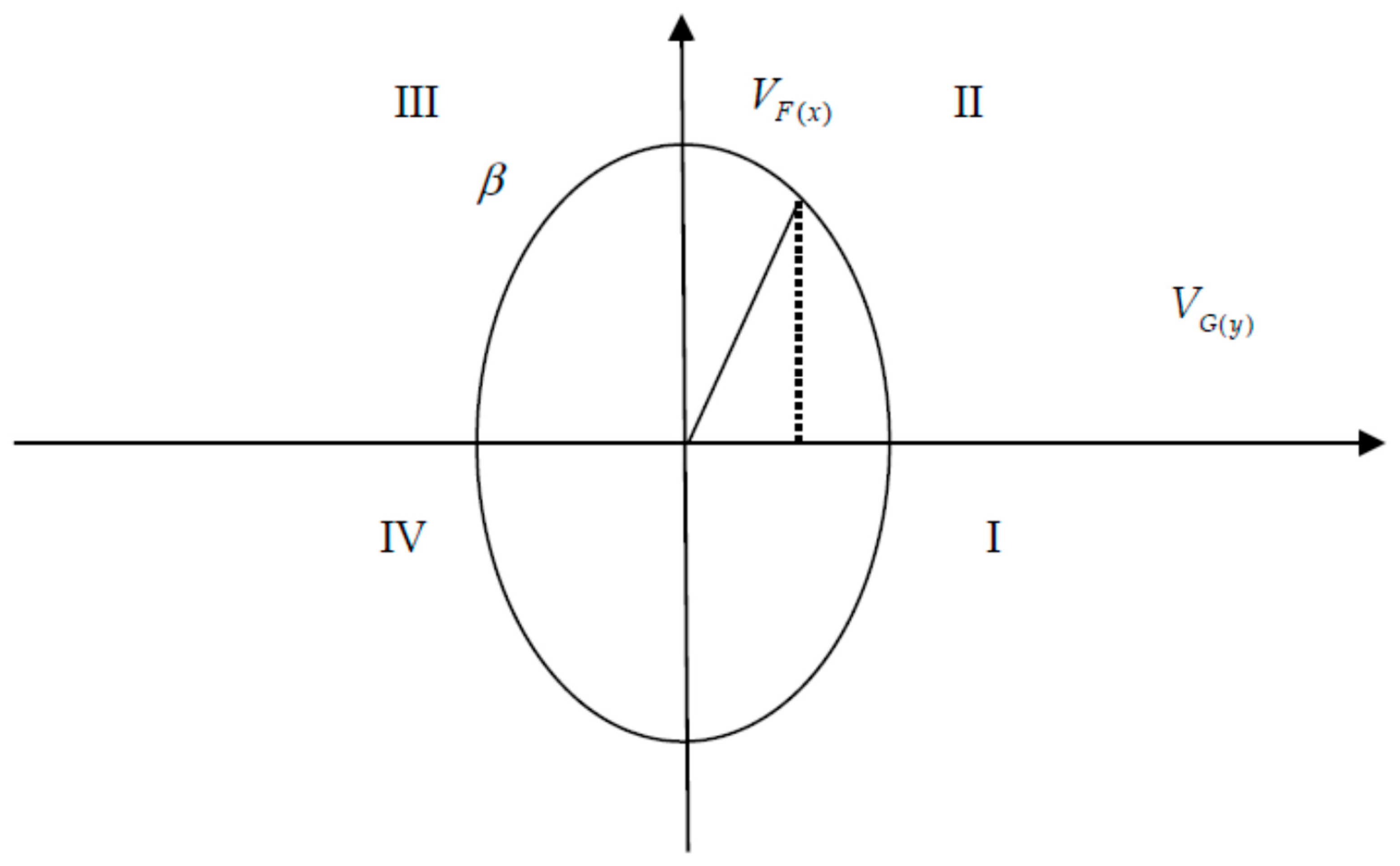
The Dynamic Coupling Coordination Degree Model (DCCDM)

The dynamic coupling coordination degree model is used to determine the coupling degree of the whole system [44].
Li et al. [45] first proposed the DCCDM and used it for coordinated evaluation between the resource environment system and the socioeconomic system, and then divided the grades of the coupling degree of the compound system.
For clarifying the relationship between sea system and land system, we assume that the sea system and the land system and their interrelationships are a compound system. In accordance with systematic evolution in the general systems theory, we establish a dynamic coupling coordination degree model between the sea system and land system to analyze the dynamic evolution and coupling states of the compound system.
The changes of sea system and land system are nonlinear, so the evolutional equation of them can be described as:
d x ( t ) / d t = f ( x 1 , x 2 , , x n ) ; i = 1 , 2 , ... , n ;
where f is the nonlinear function of x i .
The stability of the nonlinear system depends on the nature of the characteristic root of the first-order approximation system, so under the premise of ensuring the stability of motion, spreading it around the origin according to Taylor series expansion, and ignoring the high-order item, the approximate expression of the nonlinear system can be obtained:
d x ( t ) / d t = i = 1 n a i x i ; i = 1 , 2 , ... , n ;
In accordance with this idea, we can establish the general function of the change process of sea system and land system:
f ( x ) = i = 1 n a i x i * , i = 1 , 2 , ... , n
g ( y ) =   i = 1 n b i y i *    , i = 1 , 2 , ... n
Assuming the sea system and land system and their interrelationships as a single system, there are two elements F ( x ) , G ( y ) within this system. According to the Bertalanffy’s general system theory, the evolution equation for the compound system can be expressed as:
F ( x ) = d f ( x ) / d t = T 1 f ( x ) + T 2 g ( y ) , V F ( x ) = d F ( x ) / d t
G ( y ) = d G ( y ) / d t = U 1 f ( x ) + U 2 g ( y ) , V G ( y ) = d G ( y ) / d t
where F ( x ) and G ( y ) are the evolution states of sea system and land system respectively under the influence of their own and external environments. V F ( x ) and V G ( y ) are respectively the evolution speed of the sea system and the land system. In the compound system, F ( x ) and G ( y ) are mutually influenced, and the change of any subsystems will lead to the change of the whole system. The evolution speed of the system V can be regarded as a function of V F ( x ) and V G ( y ) , so V = f ( V F ( x ) , V G ( y ) ) . Therefore, taking V F ( x ) and V G ( y ) as the control variables, the coupling relationship between the whole system and two subsystems is studied by analyzing the changes of V . Since the evolution of the whole system conforms to an S-shaped mechanism, we assume that the dynamic coupling relationship between sea system and land subsystem is periodic. In each cycle, because the changes of V are caused by V F ( x ) and V G ( y ) , we analyze V by projecting the evolution trajectories of V F ( x ) and V G ( y ) in a two-dimensional plane ( V F ( x ) , V G ( y ) ) . In this condition, the variation of V is an ellipse in the coordinate system, as shown in Figure 4. The variable β expresses the angle between V F ( x ) and V G ( y ) . According to the value of β , we can determine the dynamic coupling coordination degree of the sea–land system (The specific assessment criteria and grade of β are shown in Table 4.).
β = arctan ( V F ( x ) / V G ( y ) )
In a cycle, the whole system will experience four states according to the value of β : (I) a low-grade symbiosis stage, (II) a break-in development stage, (III) an utmost development stage, (IV) a high-grade symbiosis stage.

3. Results and Discussion

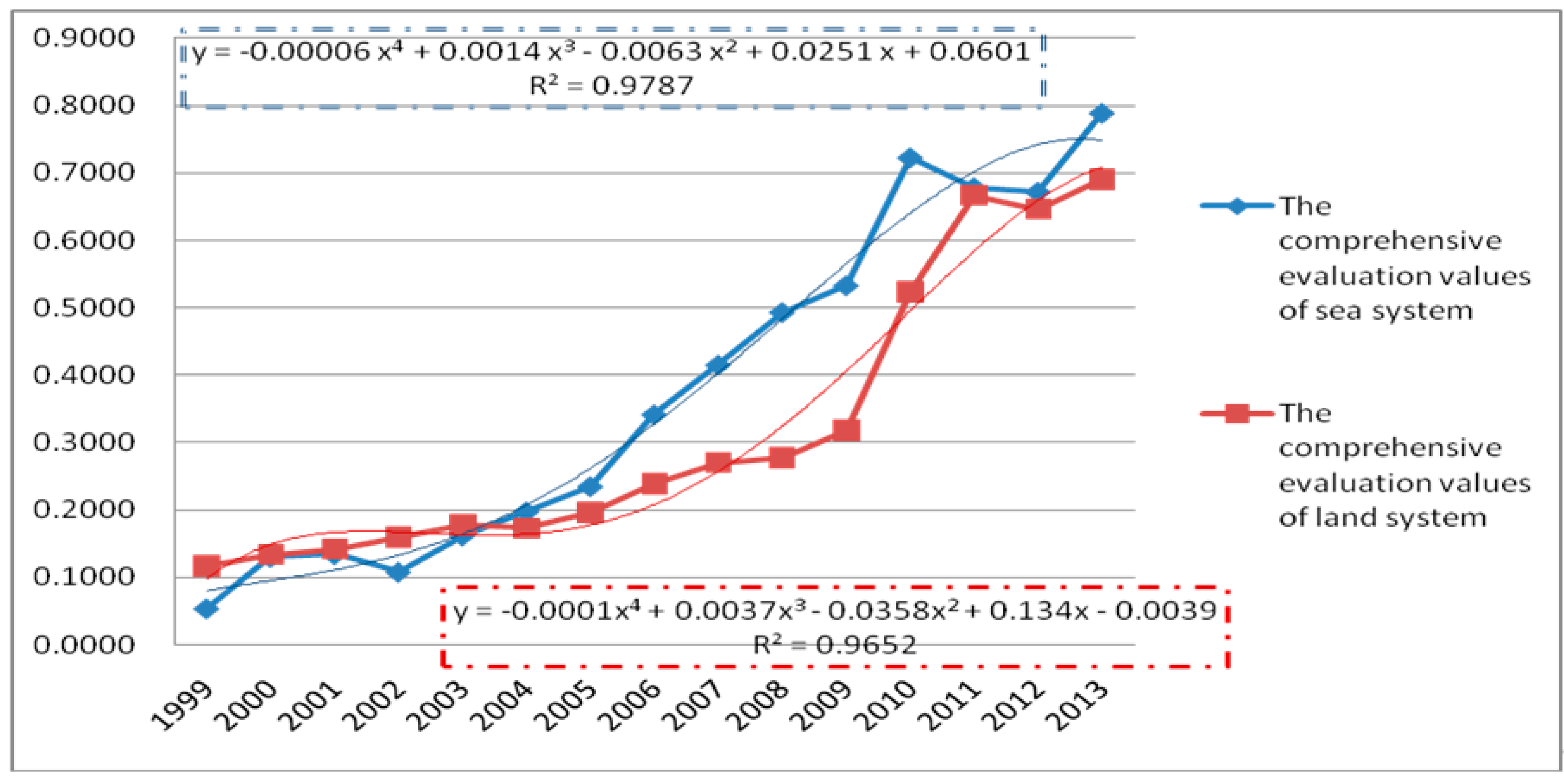
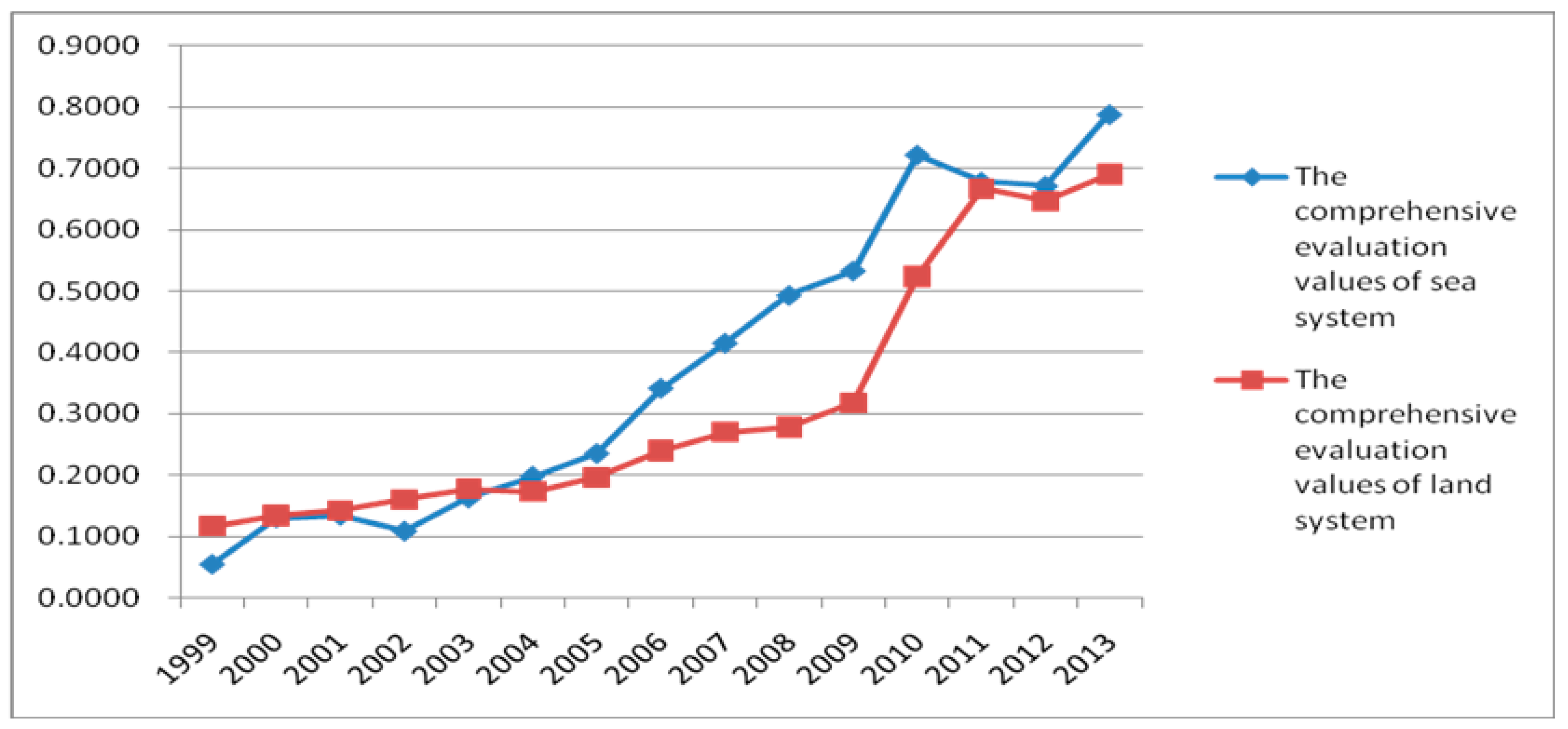
3.1. The Time Series Analysis of the Comprehensive Evaluation Values of Sea System and Land System

Firstly, the subjective weight and the objective weight are calculated by the AHP and IEW respectively. Secondly, in accordance with Equation (8), we calculate the combination weight of the evaluation indexes. Finally, we bring the normalized data and the combination weight into Equations (9) and (10), and get the comprehensive evaluation values of the sea system and the land system. See Table 2 and Table 5.
In Table 2 and Table 5, we can see that the comprehensive evaluation values of the sea system and the land system all gradually increased from 1999 to 2013 in Hainan. The comprehensive evaluation values of the sea system increased from 0.0544 to 0.7883 with growth of 0.7339 during 1999–2013, with a growth rate was 93.1%. The comprehensive evaluation values of the land system increased from 0.1169 to 0.6906 with a growth of 0.5737 during 1999–2013, with a growth rate of 83.07%. According to the different comprehensive evaluation values of sea system and land system, we divide the development of the sea–land system in Hainan into two cases: (1) f ( x ) > g ( y ) , marine economy dominant type; (2) f ( x ) < g ( y ) , land economy dominant type.
In Figure 5, we can see that the marine system of China witnessed continuous development in 1999–2013 years, and that though there was a decrease in 2011, the growth trend remained unchanged. The first year of the “12th Five-Year” plan was 2011, when the economic, social and resource indexes of the marine system were rising, but the environment index declined. For example, the amount of industrial wastewater discharged increased significantly in the coastal areas. When we focus on developing the marine economy, the external environment and its regulation are overlooked, resulting in a negative impact on marine economic development. The land economy maintained its growth in 1999–2013, except for a small decrease in 2012 which may also be caused by the destruction of the environment. During 1999–2003, f ( x ) / g ( y ) were less than 1 and gradually approaching 1, indicating that the development of the marine economy had lagged behind the land economy. In 2003, the State Council issued the “National Marine Economic Development Plan” [46], which led to a rapid development of the marine economy. However, in 2004–2013, f ( x ) / g ( y ) was greater than 1, indicating that the development of the marine economy was ahead of the land economy. In 2005, the government of the Hainan province had issued “About Accelerating the Development of the Marine Economy Decision”, the marine economy had gone through a blowout development, and the economic gap between the sea and the land widened. At the same time, the burden of the environment on the marine economy was becoming heavier. After 2011, f ( x ) / g ( y ) was stable near 1, indicating that the sea system and the land system gradually realized coordinated development.
The research results of this part are basically as same as the research results of Yang et al. [12] and Sun et al. [13]. In their research, they carried out a quantitative study on the sea–land coordination in Bohai sea ring area in China respectively, the results showed that the comprehensive evaluation values of sea system and land system are increasing steadily. Thus, with the country’s high attention to the marine economy and adhering to the sea-land coordination policy, the economic strength of the sea system and the land system indeed have a general increase.

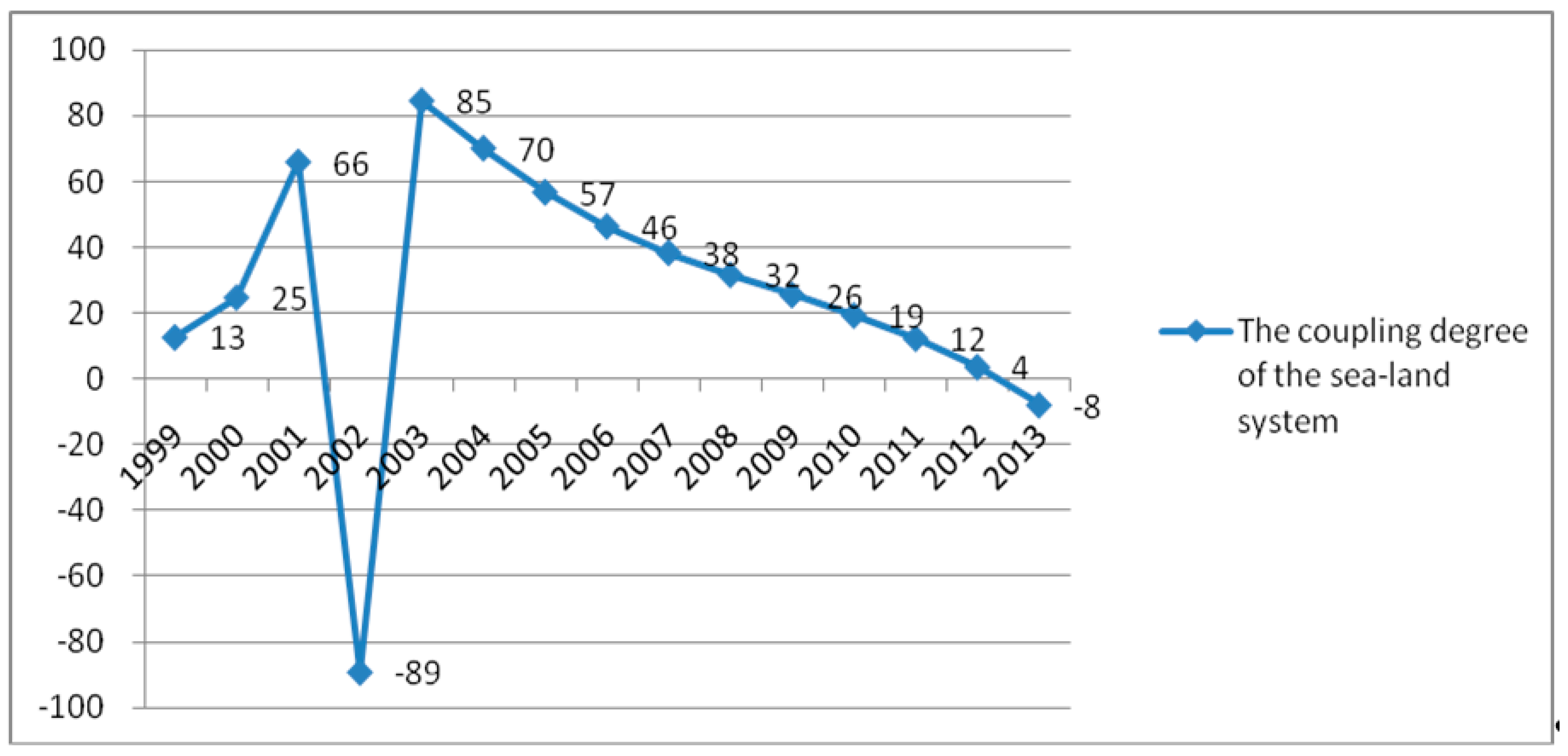
3.2. The Time Series Analysis of Coupling Coordination Degree of Sea System and Land System

In Table 6, we can see that the coupling degree C of the sea system and the land system in Hainan from 1999 to 2013 was between 0.9310 and 0.9978, and the volatility was 7.18%, so the change in that variable was relatively stable. But the coupling coordination degree D was between 0.2824 and 0.8590, a relatively apparent change. The reason for this phenomenon is that the coupling degree indicates synchronization between land system and sea system, but it does not indicate the direction of synchronization between them, while the coupling coordination degree D takes full account of the degree of good or bad coordination between them. See column three in Table 6, which shows that the coupling coordination degree of sea system and land system experienced three stages from 1999 to 2013: uncoordinated development (1999–2002), transitional development (2003–2007), and coordinated development (2008–2013).
In order to explore the effect of the comprehensive evaluation values of the sea system and the comprehensive evaluation values of the land system on the coupling coordination degree D , a multivariate linear regression model was established based on the coupling coordination degree D as the dependent variable, and the comprehensive evaluation values of the sea system and the comprehensive evaluation values of the land systems as the independent variables, using Statistical Product and Service Solutions (SPSS) software. The results are shown in Table 7 and Table 8. In Table 7, it can be seen that in this multivariate linear regression model, the fitting degree of the model R 2 is 0.993, very close to 1; this shows that the fitting degree of the model is very good. This multiple linear regression model can be expressed as: Y i ( D ) = 0.265 + 0.582 f i ( x ) + 0.223 g i ( y ) , ( i = 1 , 2 , ... , 15 ) , and it can be seen in Table 8 that the coupling coordination degree D can be expressed as a multivariate linear function of the comprehensive evaluation values of the sea system and the land system. When the comprehensive evaluation value of the sea system increases by 1 unit, the coupling coordination degree of the sea–land system increases by 0.582 units; when the comprehensive evaluation value of the land system increases by 1 unit, the coupling coordination degree of the sea–land system increases by 0.582 units.
In short, the relationship between the land system and the sea system developed in the desired direction. Also note that the overall comprehensive evaluation values of the sea system has a greater effect on the coupling coordination degree D than does the comprehensive evaluation values of the land system. The main reasons for this are that the government of Hainan Province has begun to pay attention to land economy with careful attention to the marine economy, having begun the process of developing sea–land coordination. The sea–land coordination development of Hainan Province has been inextricably linked with sustainable development policy, the scientific outlook on development policy, and the sea–land coordination policy that China has been promoting from 2003.
The research results of this part are basically the same as the research results of Zhao et al. [15]. In her research, she used the coupling coordination degree to assess the coupling coordination of sea-land system from 2003–2013, the results showed that China’s sea-land system achieved from on the verge of uncoordinated to well coordinated from 2003–2013. Thus, it can be seen that CCDM is appropriate for the study of coupling coordination degree of sea system and land system.

3.3. The Scissors Difference Analysis of Sea System and Land System

In accordance with the comprehensive evaluation values of sea system f ( x ) and land system g ( y ) , polynomial regression models are used to fit the trend functions of sea system F ( x ) and land system G ( y ) in Excel, as shown in Figure 6. Hence the following formulas:
F ( x ) = 0.00006 t 4 + 0.0014 t 3 0.0063 t 2 + 0.0251 t + 0.0601       ( R 2 = 0.9787 )
V F ( x ) = 0.00024 t 3 + 0.0042 t 2 0.0126 t + 0.0251
G ( y ) = 0.0001 t 4 + 0.0037 t 4 0.0358 t 4 + 0.134 t 0.0039              ( R 2 = 0.9652 )
V G ( y ) = 0.0004 t 3 + 0.0111 t 2 0.0716 t + 0.134
where V F ( x ) = F ( x ) = d x / d t and V G ( y ) = G ( y ) = d y / d t .
The scissors difference α between sea system and land system is calculated according to Equation (16). In Figure 7, it can be seen that the curve of the scissors difference α is a “ W ” type, which can be divided into four stages: during the first stage, from 1999 to 2000, the scissors difference α was basically showing a downward trend, decreasing from 3.2 to 1 , which indicated that the difference between sea system and land system was decreasing. The second stage was from 2001 to 2003, when the scissors difference α showed a brief upward trend. During the third stage, from 2004 to 2006, the scissors difference α showed a brief downward trend and reached its minimum in 2006; and during the fourth stage, from 2007 to 2013, the scissors difference α between the sea system and the land system gradually increased and reached its maximum in 2013.
In short, it can be seen that: from 1999–2000, the sea system was relatively backward, the land system was developing well, the pressure from the sea system to the land system had been revealed, but the development speed of land system decreased significantly, thus, at this time, Hainan Province had begun to focus on developing the sea system; from 2001 to 2006, the land system was relatively backward, the sea system was developing well, the development speed of sea system was faster than that of the land system, and the interaction between two systems was obvious. The reasons for this were, at this time, Hainan Province had begun to implement the sea–land coordination policy and the State had promulgated a series of policies and regulations to promote the sea–land coordination; from 2007 to 2013, the development speed of land system exceeded that of sea system, the restriction effects of sea system on land system were evident, thus, at this time, the sea–land coordination policy had been effectively implemented in Hainan Province.

3.4. The Dynamic Coupling Coordination Degree Analysis of the Sea–Land System Model

As can be seen in Figure 8, the dynamic coupling coordination degree of the sea–land system is basically a parabolic shape. From 1999 to 2003, except for 2002, the dynamic coupling coordination degree of the sea–land system demonstrated a general uptrend; after 2003, it was basically a downward trend. The coupling state of the sea–land system was in the break-in development stage except for in 2002. In 2002, Hainan Province was affected by Severe Acute Respiratory Syndrome (SARS), and the developments of the sea system and the land system were seriously disturbed; so in the analysis of this part, we temporarily did not consider 2002. The coupling state can therefore be divided into three stages. The primary-grade coordinated development stage was from 1999 to 2000. In this stage, the development speed of the sea system was less than that of the land system, and the development of the sea has already begun to show the stress on the development of the land. The common development stage was the second stage, which was from 2001 to 2007. During this period, with the rapid development of the sea, the sea system and the land system began to interact with each other, and the restrictions on the land from the sea began to appear, but were not prominent. The third stage was also the primary-grade coordinated development stage, from 2008 to 2013, the development speeds of the sea system and the land system had both fallen, with the declining speed of the sea system being faster than that of the land system.
Based on the above analysis, it can be seen that the results of this part are basically in agreement with the results of Section 3.3. Thus, we can know that the coupling state of the sea–land system has a lot to do with the ocean policies of Hainan and the development policies of China. At the same time, the coupling state of the sea–land system circled between the primary-grade coordinated development stage and the common development stage. This is consistent with the interpretation of the coupling state of system in the literature [47].

3.5. The Influencing Factors of Coupling Coordination Degree of Sea System and Land System

There are many factors influencing the coupling coordination degree of the sea system and land system. This paper mainly considers 16 indicators and 4 subsystems, including economic development, social progress, environmental protection, and resource efficiency. A linear regression analysis was performed between the comprehensive evaluation values of 16 indicators and 4 subsystems and the coupling coordination degree D , using SPSS software. The results are shown in Table 9 and Table 10. In the 5% confidence interval, all indicators and subsystems are significantly correlated with the coupling coordination degree D in addition to the environmental protection subsystem; the fitting degree R 2 is greater than 0.841 and is very ideal between the other subsystems and the coupling coordination degree.
In Table 9, it can be seen that the influence order of each subsystem includes resource efficiency, economic development, and social progress in the sea system, but in the land system, the influence order includes economic development, resource efficiency and social progress. (The environmental subsystem is not considered because in the linear analysis the fitting degree is less than 0.5). This suggests that social progress, economic development, and resource efficiency have positive influences on the coupling coordination degree. Although the fitting degree of environmental protection is not ideal, its positive role in promoting sea–land coordination, which has been confirmed by many scholars, cannot be ignored [48,49]. Thus, for the actual situation in Hainan, priority in the process of sea–land coordination should be given to social progress, economic development, and resource efficiency, along with strengthening the efforts and awareness of environmental protection to enhance the role of environmental protection.
In Table 10, it can be seen that in the 16 indicators in sea system, the top five influencing factors on the coupling coordination degree D are marine science and technology, GMP accounts for GDP proportion, marine capture production, gross fisheries product, and length of wharf, respectively (The top five influencing factors are marked in bold in Table 10). The mariculture area, staff and workers of marine scientific research, the direct discharge of industrial waste water into marine, the per capita area of marine nature reserves, and the number of completed projects for marine pollution control in the year, rank in the last five. For the land system, the top five are: percentage of social employed population, total investment in fixed assets, financial expenditures on education, health and science, regional economic density; growth rate of gross national product, respectively (The top five influencing factors are marked in bold in Table 10). Employees in scientific research and technological development, the afforested area, total discharge of industrial waste water, per capita arable land, and land transportation volume rank in the last five. This shows that improving the efficiency of economic development, increasing the investment in science and technology, labor and infrastructure can effectively promote the coordinated development of sea-land system in Hainan. The research results of this part are basically as same as the research results of Liang et al. [14]. In his research, he found that Guangdong Province should give priority to economic efficiency factors, social development factors and labor technology investment factors to coordinate the sea-land system.

4. Conclusions

Research on the relationship between the sea system and the land system is important for promoting the overall development of the sea–land system in Hainan Province. The coordinated development of sea system and land system is a constantly changing process. In this paper, taking the statistical data of Hainan Province from 1999 to 2013 as our example, we constructed a sea–land system which includes four subsystems—economic development, social progress, environmental protection, and resource efficiency—to measure the coupling coordination degree between the sea system and the land system. Our conclusions are as follows:
(1)
From 1999 to 2013, the comprehensive evaluation values of the sea system and the land system of Hainan Province were basically increasing step by step, and the basic development trend was consistent. Moreover, the development of sea-land system in Hainan Province had gone through two stages from 1999–2013: the land economy dominant stage and the marine economy dominant stage.
(2)
Through the analysis of the coupling coordination degree between sea system and land system, it can be seen that the relationship between them is developing in a desirable way. This shows that under the influence of national policy, the government of Hainan has begun to pay attention to the land economy as well as to the marine economy and implemented the sea-land coordination policy.
(3)
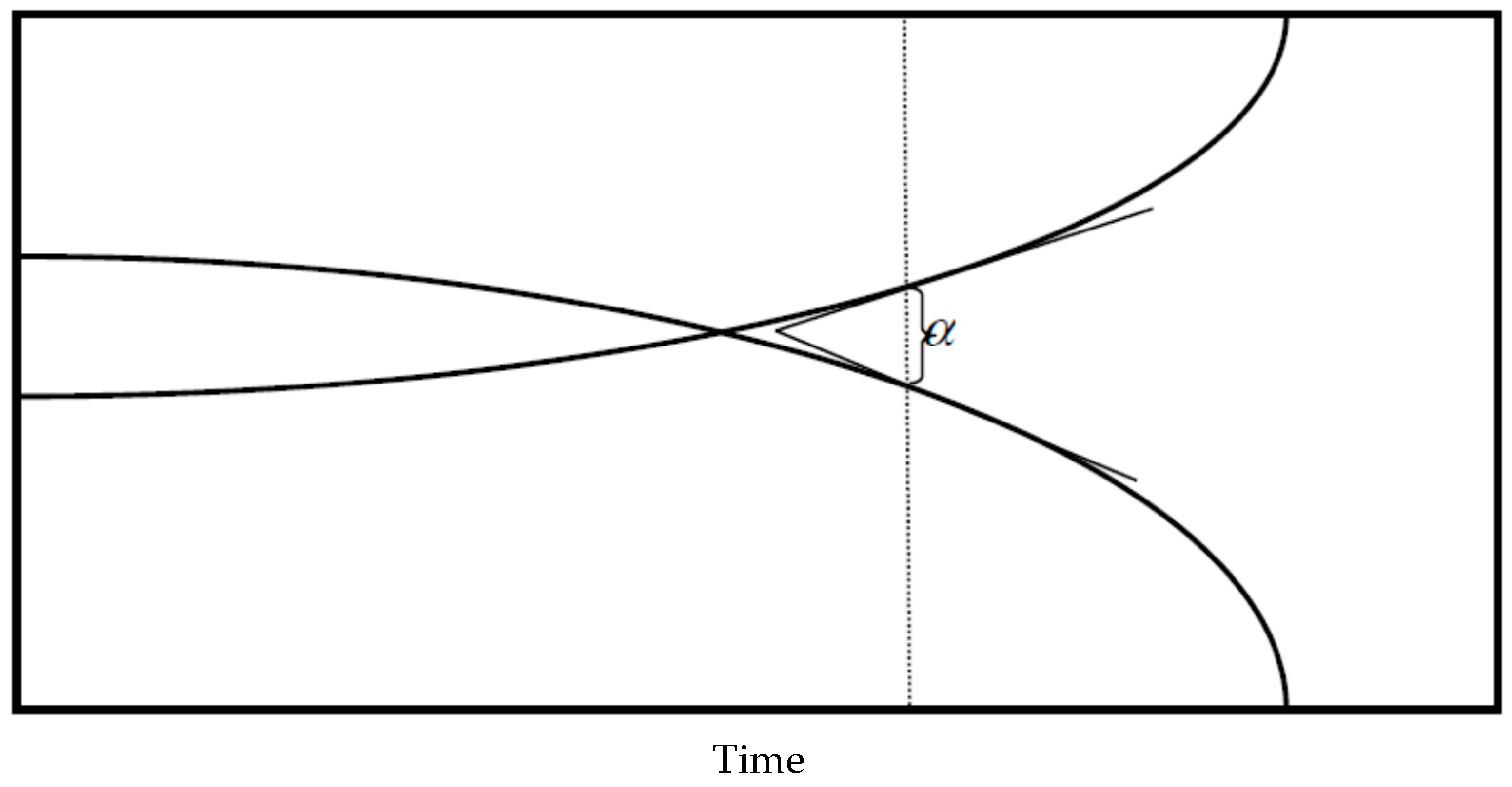
With the attention of the country and the government of Hainan to the sea-land coordination policy, the gap between the development speed of the marine economy and land economy has been increasing, and the curve of the scissors difference α is a “ W ” type.
(4)
The dynamic coupling coordination degree of the sea–land system, which follows a parabolic curve, was basically in the break-in development stage from 1999–2013. At the same time, the coupling state of the sea–land system circled between the primary-grade coordinated development stage and the common development stage.
(5)
To promote coupling coordination development of sea–land system in Hainan Province, the government should give priority to economic development, social progress, and resource efficiency subsystems in adhering to the principles of developing the sea through science and technology and of sea–land coordination, and increase efforts towards and cultivate consciousness of environmental protection, making environmental protection an important aspect of promoting sea–land coordination. What’s more, improving the efficiency of economic development, increasing the investment in science and technology, labor and the infrastructure can effectively promote the coordinated development of sea–land system in Hainan.
In building on previous studies, this paper makes a useful attempt to quantify the sea–land coordination. We hope to provide guidance for the sea–land coordination development of Hainan Province and other coastal areas and cities. However, due to the limits of statistical data in Hainan Province, the available evaluation indicators of sea–land system are limited, which leads to a relatively weak consistency in evaluation indicators between the sea system and the land system. This is a problem that needs to be solved in future study.

Acknowledgments

This paper is supported by the National Social Science Fund of China (Major Program), China, No. 13ZD162.

Author Contributions

Liming Zhao and Yujie Wu conceptualized and designed the study; Ling Li analyzed the data and wrote the paper. All authors read and approved the final manuscript.

Conflicts of Interest

The authors declare no conflict of interest.

Appendix A

Table A1. The standardized data for sea system.
YearGross Marine ProductGMP Accounts for GDP ProportionGross Fisheries ProductInternational Tourism Foreign Exchange IncomeMain Port Cargo ThroughputDistribution of Coastal ObservationStaff and Workers of Marine Scientific ResearchNumber of Marine Science and Technology
19990.0000.0000.0000.0610.0000.01370.00000.0000
20000.0190.1030.0660.0620.0200.02740.01080.0256
20010.0570.3420.1260.0630.0330.02740.02160.0513
20020.0660.3070.1160.0240.0600.00000.02700.0769
20030.1100.4950.1670.0000.0970.38360.00540.0513
20040.2000.8510.2320.0380.1230.42470.01620.0513
20050.2370.8740.3070.1900.1340.36990.01080.1026
20060.3100.9810.1870.5240.3450.28770.25950.3462
20070.3821.0000.2550.7770.5120.34250.66490.4872
20080.4520.9440.3440.8260.5440.35620.83240.4487
20090.5050.9460.4150.5720.6020.26030.87570.5641
20100.6100.8640.5070.7680.7180.54790.90270.6410
20110.7230.7970.6571.0000.8290.35620.83781.0000
20120.8420.8220.8100.8290.9100.05480.87570.5128
20131.0000.9171.0000.8311.0001.00001.00000.5256
YearDirect Discharge of Industrial Waste Water into MarineNumber of Completed Projects for Marine Pollution Control in the YearNumber of Marine Nature ReservesPer Capita Area of Marine Nature ReservesEconomic Density of CoastlineLength of WharfMarine Capture ProductionMariculture Area
19990.3900.1080.7080.007−0.0010.0000.0000.393
20000.5131.0000.7080.0060.0210.0880.1340.538
20010.6610.3240.7080.0060.0430.0880.2750.670
20020.6170.0680.0000.0000.0600.0880.4250.728
20031.0000.1350.0000.0000.0270.0880.5880.761
20040.7720.1080.0000.0000.0630.0880.7330.856
20050.4440.3240.1670.0050.1080.1760.8700.894
20060.0000.3781.0000.0100.1660.2061.0001.000
20070.3320.2161.0000.0100.2290.2430.6060.000
20080.4690.1760.9170.1960.3150.2570.6530.275
20090.8140.0681.0000.0100.4210.7270.8250.610
20100.8480.1220.7501.0000.5790.9770.7400.539
20110.4360.3110.7500.1840.7560.9770.8240.550
20120.3410.2700.7500.1850.8850.8880.9150.670
20130.3760.0000.7500.1830.9971.0000.9330.764
Table A2. The standardized data for land system.
YearGrowth Rate of Gross National ProductTotal Investment in Fixed AssetsTotal Merchandise Exports in Foreign TradeTotal Retail Sales of Social Consumer GoodsLand Transportation VolumeHousehold Disposable Income of Urban ResidentsEmployee in Scientific Research and Technological DevelopmentFinancial Expenditure in Education, Health and Science
19990.00000.0000.0000.0000.0940.0000.1050.000
20000.15900.0010.0180.0180.0840.0010.1530.005
20010.12400.0060.0180.0370.0300.0280.2000.013
20020.18800.0140.0240.0570.0000.0840.0000.026
20030.16500.0340.0410.0420.0680.1090.0130.034
20040.17100.0530.1160.0970.1170.1360.0970.051
20050.14100.0750.0930.1390.1840.1580.2850.081
20060.27600.0930.2390.1910.3230.2310.3100.102
20070.41200.1260.3680.2620.4300.3220.2970.177
20080.11800.2050.3770.3750.3100.4130.3870.272
20090.12900.3200.3890.4670.3040.4780.4780.403
20101.00000.4500.5550.5730.6110.5820.7450.522
20110.84700.5610.6060.7170.7430.7410.8040.716
20120.31800.7710.8090.8530.9010.8860.9020.890
20130.14101.0001.0001.0001.0001.0001.0001.000
YearTotal Discharge of Industrial Waste WaterIndustrial Solid Waste GenerationPollution Control Project InvestmentAfforested AreaRegional Economic DensityPer capita Arable LandTotal Energy ProductionPercentage of Social Employed Population
19990.9631.0000.0020.072−0.0010.9840.0000.009
20000.9650.9260.0190.0980.0190.9110.0080.000
20010.9670.9840.0000.3830.0400.7790.0120.000
20020.9740.9580.2600.1570.0650.6960.0090.075
20030.9610.9380.0041.0000.0810.5760.0060.129
20040.9810.8970.0010.3760.1210.4870.0010.164
20050.9610.8350.0910.3290.1590.4010.0100.185
20060.9550.7780.1820.1940.2140.2970.0150.151
20071.0000.7470.0080.0290.2850.1900.0200.248
20080.9990.5710.0070.0920.3790.3920.0350.257
20090.9660.6250.0070.1250.4360.2930.0390.340
20100.0130.5940.0090.0750.5910.0640.8640.403
20110.0440.0001.0000.0720.7640.0710.9570.523
20120.0000.0990.1620.0470.8900.0431.0000.766
20130.0290.0400.0510.0001.0000.0040.8981.000

References

  1. Pajaro, M.G.; Mulrennan, M.E.; Vincent, A.C.J. Toward an integrated marine protected areas policy: Connecting the global to the local. Environ. Dev. Sustain. 2010, 12, 945–965. [Google Scholar] [CrossRef]
  2. Smith, H.D. The industrialization of the world ocean. Ocean Coast. Manag. 2000, 43, 11–28. [Google Scholar] [CrossRef]
  3. Theory and Practice. Decision of the Central Committee of the Communist Party of China on Several Issues of Perfecting the Socialist Mark Economic System; People’s Publishing House: Beijing, China, 2003. (In Chinese) [Google Scholar]
  4. Xi, J.P. A note on the proposal of the CPC Central Committee on the formulation of the thirteenth five-year plan for national economic and social development. Pract. Theory Thought 2015, 11, 24–31. (In Chinese) [Google Scholar]
  5. Zhang, H.F. A discussion on the integration of sea-land co-planning to build a powerful country. Pac. J. 2005, 7, 14–17, (In Chinese with English Abstract). [Google Scholar]
  6. Cincin-Sain, B.; Belfiore, S. Linking marine protected areas to integrate coastal and ocean management: A review of theory and practice. Ocean Coast. Manag. 2005, 48, 847–868. [Google Scholar] [CrossRef]
  7. Panayotou, K. Coastal management and climate change: an Australian perspective. J. Coast. Res. 2009, 1, 742–746. [Google Scholar]
  8. Mitchell, C.L. Sustainable oceans development: The Canadian approach. Mar. Policy 1998, 22, 393–412. [Google Scholar] [CrossRef]
  9. Han, Z.L.; Di, Q.B.; Zhou, L.P. Discussion on the connotation and target of sea–land coordination. Mar. Econ. 2012, 1, 10–15, (In Chinese with English Abstract). [Google Scholar]
  10. Ye, X.D. Constructing “Digital Ocean” to implement sea–land coordination. Pac. J. 2007, 4, 77–86. (In Chinese) [Google Scholar]
  11. Wang, L. Achievements, problems and prospects of land and sea-land co-ordination development. Macroecon. Manag. 2013, 9, 23–24. (In Chinese) [Google Scholar]
  12. Yang, Y.D.; Sun, C.Z. Assessment of land-sea coordination in the Bohai sea ring area and spatial-temporal differences. Resour. Sci. 2014, 4, 691–701, (In Chinese with English Abstract). [Google Scholar]
  13. Sun, C.Z.; Gao, Y.; Han, J. Sea & land economy integration assessment based on competence structure relation model in the Bohai Sea ring area. Areal Res. Dev. 2012, 12, 28–33, (In Chinese with English Abstract). [Google Scholar]
  14. Liang, J.J.; Yang, M.Z. Analyzing and evaluating Guangdong’s coupling coordination and evolution of the land-sea system. Mar. Econ. 2015, 8, 42–48, (In Chinese with English Abstract). [Google Scholar]
  15. Zhao, X.; Nan, X. A study of the coupling coordination mechanism between marine and land economy from the perspective of the giant system. Ecol. Econ. 2016, 8, 25–35. [Google Scholar]
  16. Fan, F.; Sun, C.Z. Research on the cooperation development of marine & inland economy in Liaoning Province. Areal Res. Dev. 2011, 2, 59–63, (In Chinese with English Abstract). [Google Scholar]
  17. Jiang, B.G.; Han, L.M. Strategies for building Shandong Peninsula Blue Economic Zone. J. Shandong Univ. 2009, 5, 92–96, (In Chinese with English Abstract). [Google Scholar]
  18. Chang, Y.M.; Cheng, C.C. Spatial-temporal evolution of regional economic pattern in Anhui Province. Areal Res. Dev. 2012, 4, 34–36, (In Chinese with English Abstract). [Google Scholar]
  19. Ye, B.; Li, J.Q. Studies on the optimizing strategy of the structure of marine industry in Hainan. J. Huazhong Normal Univ. 2011, 45, 125–128, (In Chinese with English Abstract). [Google Scholar]
  20. Wu, R.; Wang, D.U. Analysis of marine ecology and environmental protection in Hainan. Ocean Dev. Manag. 2013, 9, 61–65. (In Chinese) [Google Scholar]
  21. Zhang, G.H.; Wang, J. Ecological risk assessment and early warning mechanism for tourism development in Hainan Province. Trop. Geogr. 2013, 1, 88–95, (In Chinese with English Abstract). [Google Scholar]
  22. Yang, W. Administrative arrangements and displacement compensation in top-down tourism planning—A case from Hainan Province, China. Tour. Manag. 2007, 28, 70–82. [Google Scholar]
  23. Pittman, J.; Armitage, D. Governance across the land-sea interface: A systematic review. Environ. Sci. Policy 2016, 64, 9–17. [Google Scholar] [CrossRef]
  24. Li, M.; Jin, F.; Song, Z.; Liu, Y. Spatial coupling analysis of regional economic development and environmental pollution in China. J. Geogr. Sci. 2013, 23, 525–537. [Google Scholar]
  25. Wang, Q.; Yang, Y. The research of marine economy and land economy overall planning based on symbiosis theory. Chin. Fish. Econ. 2016, 5, 26–34, (In Chinese with English Abstract). [Google Scholar]
  26. Liu, X.M.; Zhang, Y.N.; Fan, L. A study on the influential factors of the overall development of marine & land economy of Shandong Province. Technol. Innov. Manag. 2017, 2, 136–144, (In Chinese with English Abstract). [Google Scholar]
  27. Gai, M.; Liu, W.; Tian, C. Spatial-temporal coupling on marine and land industrial systems in coastal regions of China. Resour. Sci. 2013, 35, 966–976, (In Chinese with English Abstract). [Google Scholar]
  28. Ding, L.; Zhao, W.; Huang, Y.; Cheng, S. Research on the Coupling Coordination Relationship between urbanization and the air environment: A case study of the area of Wuhan. Atmosphere 2015, 6, 1539–1558. [Google Scholar] [CrossRef]
  29. Ai, J.Y.; Feng, L.; Dong, X.W.; Zhu, X.D. Exploring coupling coordination between urbanization and ecosystem quality (1985–2010): A case study from Lianyungang City, China. Front. Earth Sci. 2016, 10, 527–545. [Google Scholar] [CrossRef]
  30. Wang, S.J.; Ma, H.T.; Zhao, Y.B. Exploring the relationship between urbanization and the Eco-environment—A case study of Beijing-Tianjin-Hebei region. Ecol. Indic. 2014, 45, 171–183. [Google Scholar] [CrossRef]
  31. Ishizaka, A.; Labib, A. Review of the main developments of the analytic hierarchy process. Expert Syst. Appl. 2011, 39, 14336–14345. [Google Scholar] [CrossRef]
  32. Stefanidis, S.; Stathis, D.R. Assessment of flood hazard based on natural and anthropocentric factors using analytic hierarchy process (AHP). Nat. Hazards 2013, 68, 569–585. [Google Scholar] [CrossRef]
  33. Yan, J.H.; Feng, C.H.; Li, L. Sustainability assessment of machining process based on extension theory and entropy weight approach. Int. J. Adv. Manuf. Technol. 2014, 71, 1419–1431. [Google Scholar] [CrossRef]
  34. Jesmin, F.K.; Sharif, M.B. Weighted entropy for segmentation evaluation. Opt. Laser Technol. 2014, 57, 236–242. [Google Scholar]
  35. Lai, C.; Chen, X.; Wang, Z.; Wu, X. A fuzzy comprehensive evaluation model for flood risk based on the combination weight of game theory. Nat. Hazards 2015, 77, 1243–1259. [Google Scholar] [CrossRef]
  36. Liao, C.B. Quantitative judgment and classification system for coordinated development of environment an economy. Top. Geogr. 1999, 2, 171–177, (In Chinese with English Abstract). [Google Scholar]
  37. Zhou, Z.L.; Cao, Q.Q. Coupling coordination degree model of oil-economy-environment system in the western region. In Proceedings of the 2014 International Conference on Management Science and Engineering, Helsinki, Finland, 17–19 August 2014; IEEE: New York, NY, USA, 2014; pp. 827–832. [Google Scholar]
  38. Zhou, D.; Xu, J.; Lin, Z. Conflict or coordination? Assessing land use multi-functionalization using production-living-ecology analysis. Sci. Total Environ. 2016, 577, 136–147. [Google Scholar] [CrossRef] [PubMed]
  39. Li, Q.; Su, Y.; Pei, Y. Research on coupling coordination degree model between upstream and downstream enterprises. In Proceedings of the 2008 International Conference on Information Management, Innovation Management and Industrial Engineering, Taipei, Taiwan, 19–21 December 2008. [Google Scholar] [CrossRef]
  40. Tang, Z. An integrated approach to evaluating the coupling coordination between tourism and the environment. Tour. Manag. 2015, 46, 11–19. [Google Scholar] [CrossRef]
  41. Yuan, Y.Q.; Jin, M.Z.; Ren, J.F.; Hu, M.; Ren, P.Y. The dynamic coordinated development of a regional environment-tourism-economy system: A case study from western Hunan Province, China. Sustainability 2014, 6, 5231–5251. [Google Scholar] [CrossRef]
  42. Seton, F. Scissor crises, value-prices, and the movement of value-prices under technical change. Struct. Chang. Econ. Dyn. 2000, 11, 13–24. [Google Scholar] [CrossRef]
  43. Yue, D.; Xu, X.; Li, Z.; Hui, C.; Li, W.; Yang, H.; Ge, J. Spatiotemporal analysis of ecological footprint and biological capacity of Gansu, China 1991–2015: Down from the environmental cliff. Ecol. Econ. 2006, 58, 393–406. [Google Scholar] [CrossRef]
  44. Li, X.J.; Tao, J.G. The dynamic coupling analysis for coordinated development of the environment and economy based on cloud model: Case study of Henan. In Proceedings of the 2014 International Conference on Management Science & Engineering, Helsinki, Finland, 17–19 August 2014; IEEE: New York, NY, USA, 2014; pp. 726–735. [Google Scholar]
  45. Li, C.M. Study of coordinated development model and its application between the economy and resources environment in small town. Syst. Eng. Theory Pract. 2004, 11, 134–144, (In Chinese with English Abstract). [Google Scholar]
  46. Wang, Z.K. The state council approved the implementation of the “National Marine Economic Development Plan“. Mar. Inf. 2003, 3, 31. [Google Scholar]
  47. Zhao, Y.; Wang, S.; Zhou, C. Understanding the relation between urbanization and the eco-environment in China’s Yangtze River Delta using an improved EKC model and coupling analysis. Sci. Total Environ. 2016, 571, 862–875. [Google Scholar] [CrossRef] [PubMed]
  48. Ioppolo, G.; Saija, G.; Salomone, R. From coastal management to environmental management: The sustainable eco-tourism program for the mid-western coast of Sardinia. Land Use Policy 2013, 31, 460–471. [Google Scholar] [CrossRef]
  49. Marotta, L.; Ceccaroni, L.; Matteucci, G.; Rossini, P.; Guerzoni, P. A decision-support system in ICZM for protecting the ecosystems: Integration with the habitat directive. J. Coast. Conserv. 2011, 15, 393–405. [Google Scholar] [CrossRef]
Figure 1. A conceptual rendering of sea–land coordination.
Sustainability 09 00859 g001
Figure 2. The interaction mechanism of sea system and land system.
Sustainability 09 00859 g002
Figure 3. The sketch map of the scissors difference model.
Sustainability 09 00859 g003
Figure 4. Process of coupling state of sea–land system.
Sustainability 09 00859 g004
Figure 5. The comprehensive evaluation values of the sea system and the land system.
Sustainability 09 00859 g005
Figure 6. The fitting functions of sea system and land system.
Sustainability 09 00859 g006
Figure 7. The scissors difference between the sea system and the land system.
Sustainability 09 00859 g007
Figure 8. The dynamic coupling coordination degree of the sea–land system.
Sustainability 09 00859 g008
Table 1. The advantages and disadvantages of developing sea–land coordination and integrated coastal zone management (ICZM).
The Advantages and Disadvantages of Developing Sea–Land Coordination in China
The advantages1. The rapid development of the marine economy has laid a solid material foundation for the implementation of sea–land coordination.
2. The Chinese government attaches great importance to sea–land coordination, and has upgraded sea–land coordination to a national strategy.
3. In academic circles, the research on the sea–land coordination has made some achievements, which provides a theoretical guidance for the sea–land coordination.
4. The main adviser of the sea-land coordination policy is the Chinese government, which provides an effective guarantee for the smooth implementation of this policy.
The disadvantages1. The coordination between governments at all levels is difficult.
2. Disputes over the maritime boundaries have affected the process of the sea–land coordination internationally.
3. Due to historical reasons and lack of publicity, at present the concept of “heavy land light sea” is serious, and the national awareness of developing the sea economy is weak.
4. The legal system of sea–land coordination has not yet formed.
The advantages and disadvantages of ICZM
The advantages1. At present, there are many achievements in the ICZM at home and abroad, which lay a solid foundation for the future research.
2. The dynamic assessment of the ICZM has formed a mature index assessment system, which can be expressed specifically as DPSIR model (drive-pressure-status-influence-reaction).
3. A variety of new technologies or methods have been routinely used in the ICZM research, such as Geographic Information System (GIS), Remote sensing, Decision Support Systems, Visual database, Ocean Geographic Techniques and so on.
The disadvantages1. At present, there is no uniform definition of the coastal zone at home and abroad, so the scope of ICZM cannot be well defined, leading to legislative difficulties in the coastal zone.
2. The main disciplines of ICZM research are distributed in the fields of environmental science, ecology, oceanography, geography and other natural sciences, and the social science research is less; it mainly focuses on the international relations law.
3. The funding support to ICZM is less; much of the funding comes from the international organizations.
4. The ICZM focuses on the planning process, the evaluation of the effect after the implementation of ICZM is insufficient, leading experience of ICZM cannot be well studied.
Table 2. The evaluation indexes system of sea system and land system.
System GradeSubsystem GradeBasic Grade u A H P u I E W u C W
Sea SystemEconomic developmentX1: Gross Marine Product (100 million CNY)0.12940.05680.0884
X2: GMP accounts for GDP proportion (%)0.04580.02450.0337
X3: Gross fisheries product (100 million CNY)0.09150.04740.0664
X4: International tourism foreign exchange income (USD 10,000)0.06470.06550.0644
Social progressX5: Main port cargo throughput (10,000 tons)0.09010.06520.0755
X6: Distribution of coastal observation stations (number)0.05760.05940.0579
X7: Staff and workers of marine scientific research (person)0.12750.15260.1398
X8: Number of marine science and technology (number)0.03320.04890.0414
Environmental protectionX9: Direct discharge of industrial waste water into marine (million tons)0.05200.01990.0339
X10: Number of completed projects for marine pollution control in the year (unit)0.03680.05510.0464
X11: Number of marine nature reserves (unit)0.01360.04120.0285
X12: Per capita area of marine nature reserves (m2)0.02350.19250.1154
Resource efficiencyX13: Economic density of coastline (100 million CNY/km)0.09750.08230.0881
X14: Length of wharf (m)0.02810.06990.0506
X15: Marine capture production (tons)0.06890.02230.0427
X16: Mariculture area (hm2)0.03980.01690.0269
Land SystemEconomic developmentX17: Growth rate of gross national product (%)0.13700.04420.0858
X18: Total investment in fixed assets (100 million CNY)0.06190.08070.0723
X19: Total merchandise exports in foreign trade (ten thousand US dollars)0.03570.05940.0488
X20: Total retail sales of social consumer goods (10 thousand CNY)0.09680.05800.0754
Social progressX21: Land transportation volume (10,000 tons)0.12830.04850.0843
X22: Household disposable income of urban residents (CNY)0.09070.05240.0696
X23: Employee in scientific research and technological development (person)0.03700.04240.0400
X24: Financial expenditure in education, health and science (10 thousand CNY)0.05240.07560.0652
Environmental protectionX25: Total discharge of industrial waste water (10,000 tons)0.04340.03210.0372
X26: Industrial solid waste generation (10,000 tons)0.04800.02260.0340
X27: Pollution control project investment (million CNY)0.02110.14440.0891
X28: Afforested area (ha.)0.01350.06210.0403
Resource efficiencyX29: Regional economic density (100 million CNY/km2)0.09680.05390.0731
X30: Per capita arable land(hm2)0.02530.03730.0319
X31: Total energy production (10,000 tons of standard coal)0.06850.13190.1035
X32: Percentage of social employed population (%)0.04380.05470.0498
Table 3. Discriminating standards of the coupling coordination degree.
Section D ValueTypes
Uncoordinated Development0~0.09Extremely uncoordinated
0.10~0.19Seriously uncoordinated
0.20~0.29Moderately uncoordinated
0.30~0.39Slightly uncoordinated
Transitional Development0.40~0.49On the verge of uncoordinated
0.50~0.59Barely coordinated
Coordinated Development0.60~0.69Slightly coordinated
0.70~0.79Moderately coordinated
0.80~0.89Well coordinated
0.90~1.00Quality coordinated
Table 4. The coupling degree of the sea–land model.
The Range of β StageDevelopment StageThe Performance
90 < β 0 Ilow-grade symbiosis stageDuring this period, the development speed of sea system is slow, and it is not restricted by land system. The impact of the sea system on the land system is almost zero.
0 < β < 45 IIprimary-grade coordinated development stage V F ( x ) < V G ( y ) , the development speed of the sea system is less than that of the land system, and the sea system has already begun to show the stress on the land system.
β = 45 harmonious development stage V F ( x ) = V G ( y ) , the development speed of the sea system is equal to that of the land system. It is harmonious between the sea system and the land system.
45 < β 90 common development stage V F ( x ) > V G ( y ) , with the rapid development of the sea system, the two system began to interact with each other, and the restriction of the land system to the sea system began to appear, but it is not prominent.
90 < β 180 IIIutmost development stageWith the rapid development of the marine economy, the sea system has accelerated the demand for land resources, the contradiction between the sea system and the land system has become increasingly prominent, which has restricted the development of the marine economy.
180 < β 90 IVhigh-grade symbiosis stageThe restriction between the sea system and the land system has been gradually transformed into mutual promotion, and finally reaches a high-grate symbiosis between the sea system and the land system.
Table 5. The comprehensive evaluation values of sea system and land system.
YearThe Comprehensive Evaluation Values of Sea System ( f ( x ) )The Comprehensive Evaluation Values of Land System ( g ( y ) )
19990.05440.1169
20000.13040.1339
20010.13460.1419
20020.10840.1601
20030.16250.1775
20040.19800.1730
20050.23540.1959
20060.34180.2391
20070.41530.2700
20080.49330.2774
20090.53310.3177
20100.72250.5238
20110.67830.6667
20120.67170.6464
20130.78830.6906
Table 6. The coupling coordination degree of sea system and land system.
YearCoupling Degree C Coupling Coordination Degree D Grade of Coupling Coordination
19990.93100.2824Moderately uncoordinated
20000.99990.3635Slightly uncoordinated
20010.99970.3718Slightly uncoordinated
20020.98130.3630Slightly uncoordinated
20030.99900.4121On the verge of uncoordinated
20040.99770.4302On the verge of uncoordinated
20050.99580.4634On the verge of uncoordinated
20060.98420.5347Barely coordinated
20070.97730.5787Barely coordinated
20080.95990.6082Slightly coordinated
20090.96740.6415Slightly coordinated
20100.98720.7843Moderately coordinated
20111.00000.8200Well coordinated
20120.99980.8117Well coordinated
20130.99780.8590Well coordinated
Table 7. The model summary of multiple linear regression model.
Model Summary
ModelRR2Adjusted R2Standard Estimation ErrorChange the StatisticsDurbin–Watson
R2 ChangesF Changesdf1df2Sig. F Changes
10.996 a0.993 b0.9920.01766380.993824.4592120.0000.979
a R denotes the multiple correlation coefficient; b R2 denotes the fitting degree of the model.
Table 8. The coefficients of multiple linear regression model.
Coefficient
ModelNon-Normalized CoefficientsNormalized CoefficientstSig.The Colinearity Statistics
BNormalized ErrorTrial VersionToleranceVIF
constant a0.2650.009 31.0050.000
the comprehensive evaluation values of sea system a0.5820.0520.76711.0790.0000.1267.955
the comprehensive evaluation values of land system a
The coupling coordination degree D b
0.2230.0640.2423.4920.0040.1267.955
a Predictive variable: constant, the comprehensive evaluation values of sea system, the comprehensive evaluation values of land system. b Dependent variable: the coupling coordination degree D .
Table 9. The influence order of four subsystems.
System GradeInfluencing FactorThe Linear Regression EquationThe Fitting Degree R 2 Influence Order
The sea systemEconomic Development Y i ( D ) = 0.293 + 2.459 f E C i ( x ) 0.9662
Social Progress Y i ( D ) = 0.346 + 1.750 f S O i ( x ) 0.9333
Environmental Protection Y i ( D ) = 0.390 + 2.714 f E N i ( x ) 0.244
Resource Efficiency Y I ( D ) = 0.270 + 3.135 f R E i ( x ) 0.9191
The land systemEconomic Development Y i ( D ) = 0.353 + 2.483 g E C i ( y ) 0.9531
Social Progress Y i ( D ) = 0.364 + 2.185 g S O i ( y ) 0.0923
Environmental Protection Y i ( D ) = 0.862 4.497 g E N i ( y ) 0.484
Resource Efficiency Y i ( D ) = 0.365 + 2.423 g R E i ( y ) 0.8142
Remarks: The EC denotes the economic development subsystem, the SO denotes social progress subsystem; the EN denotes environmental protection subsystem; the RE denotes resource efficiency subsystem, the i = 1 , 2 , ... , 15 .
Table 10. The influence order of 16 indicators.
Index Evaluation SystemInfluence OrderIndex Evaluation SystemInfluence Order
X1: Gross Marine Product (100 million CNY)10X17: Growth rate of gross national product (%)5
X2: GMP accounts for GDP proportion (%)2X18: Total investment in fixed assets (100 million CNY)2
X3: Gross fisheries product (100 million CNY)4X19: Total merchandise exports in foreign trade (ten thousand US dollars)11
X4: International tourism foreign exchange income (USD 10,000)8X20: Total retail sales of social consumer goods (10 thousand CNY)10
X5: Main port cargo throughput (10,000 tons)9X21: Land transportation volume (10,000 tons)12
X6: Distribution of coastal observation stations (number)7X22: Household disposable income of urban residents (CNY)8
X7: Staff and workers of marine scientific research (person)15X23: Employee in scientific research and technological development (person)15
X8: Number of marine science and technology (number)1X24: Financial expenditure in education, health and science (10 thousand CNY)3
X9: Direct discharge of industrial waste water into marine (million tons)14X25: Total discharge of industrial waste water (10,000 tons)14
X10: Number of completed projects for marine pollution control in the year (unit)12X26: Industrial solid waste generation (10,000 tons)6
X11: Number of marine nature reserves (unit)6X27: Pollution control project investment (million CNY)7
X12: Per capita area of marine nature reserves (m2)13X28: Afforested area (ha.)16
X13: Economic density of coastline (100 million CNY/km)11X29: Regional economic density (100 million CNY/km2)4
X14: Length of wharf (m)5X30: Per capita arable land(hm2)13
X15: Marine capture production (tons)3X31: Total energy production (10,000 tons of standard coal)9
X16: Mariculture area (hm2)16X32: Percentage of social employed population (%)1

