Long Term Quantification of Climate and Land Cover Change Impacts on Streamflow in an Alpine River Catchment, Northwestern China


Abstract
:1. Introduction
2. Materials
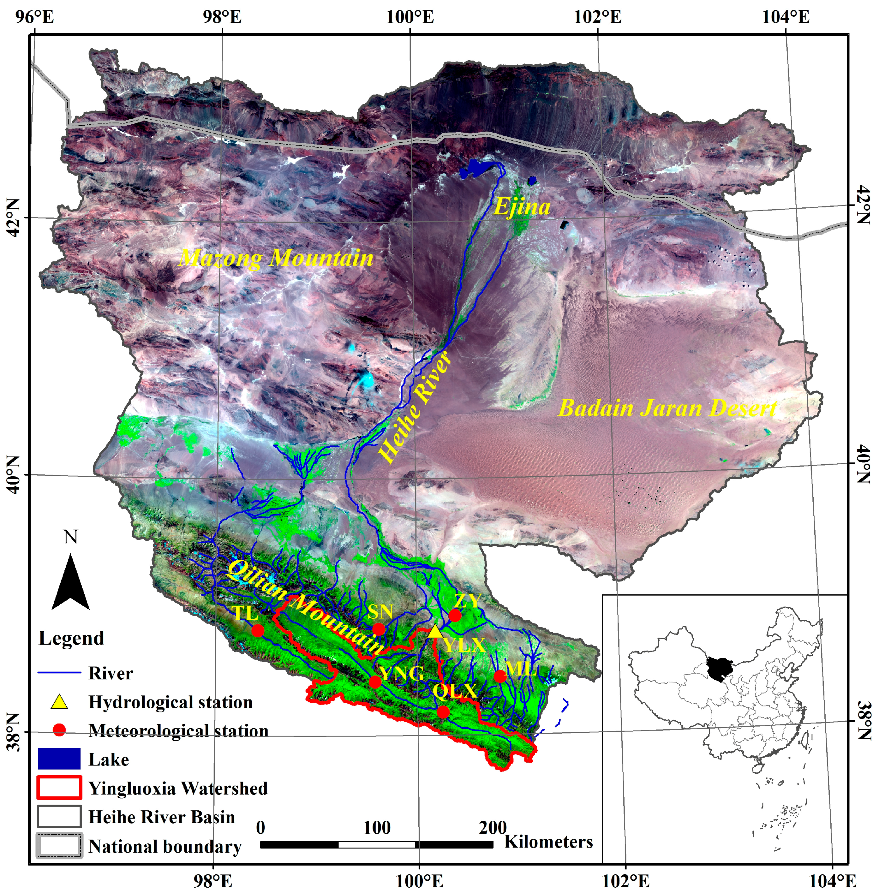
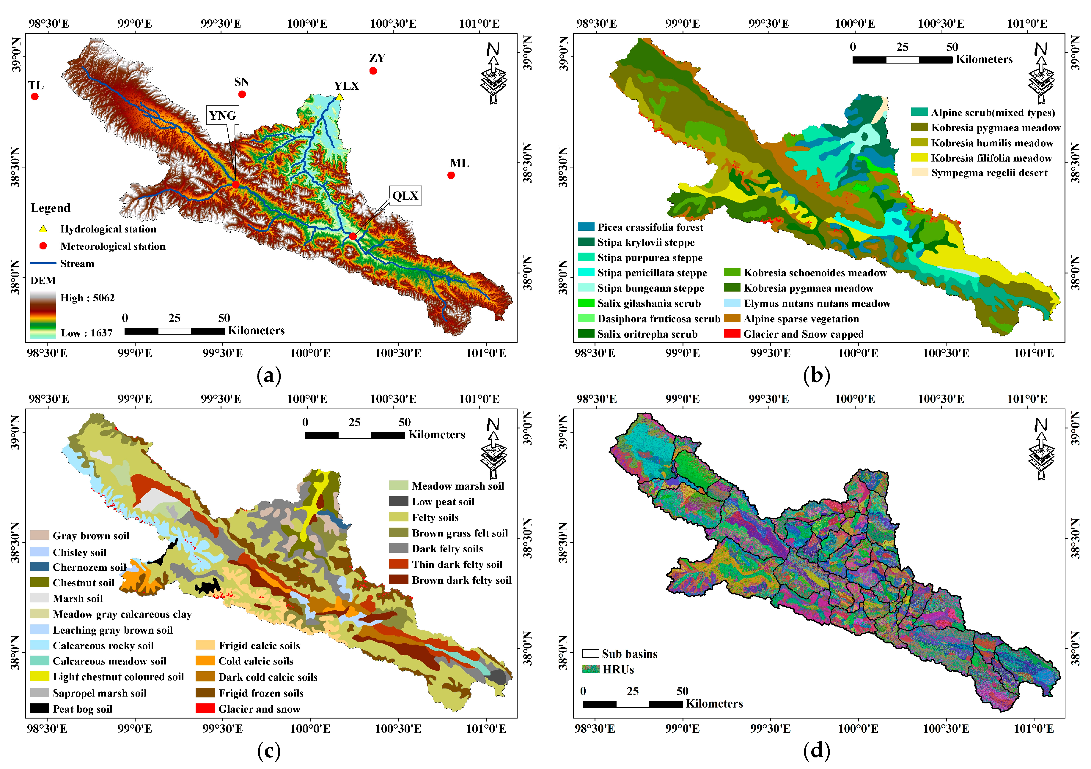
2.1. Study Area
2.2. Data Availability
3. Methodologies
3.1. Distinguishing the Impacts of Climate and Land Cover Changes
3.2. Soil and Water Assessment Tool (SWAT) Model and Model Setup
3.3. Model Calibration and Confirmation Analysis
3.4. Mann-Kendall Trend Test
4. Results and Discussion
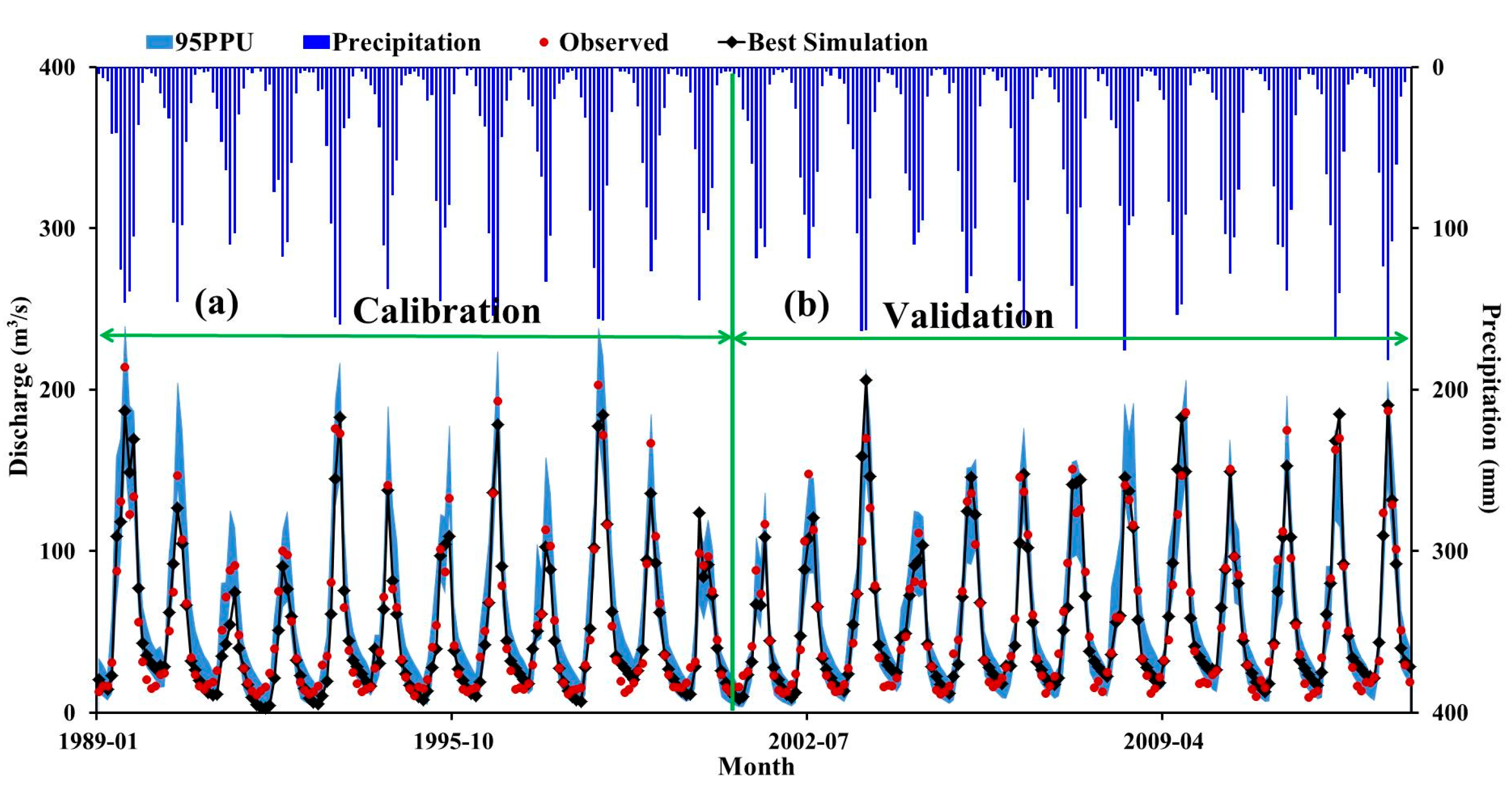
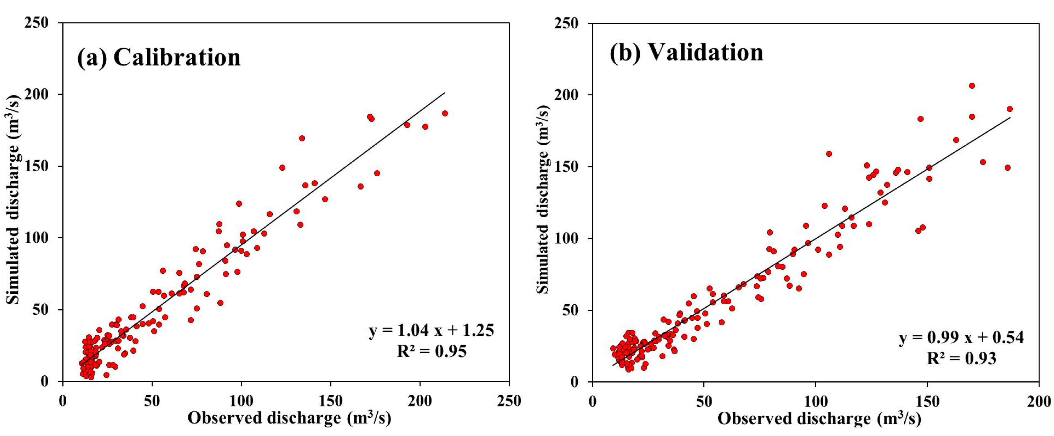
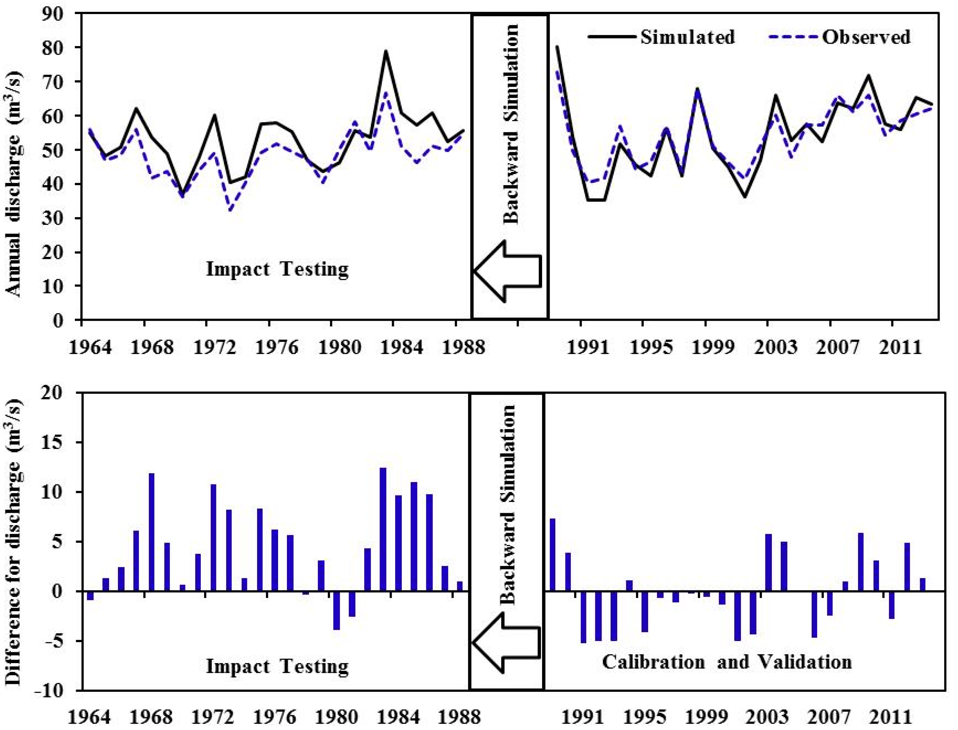
4.1. Model Performance
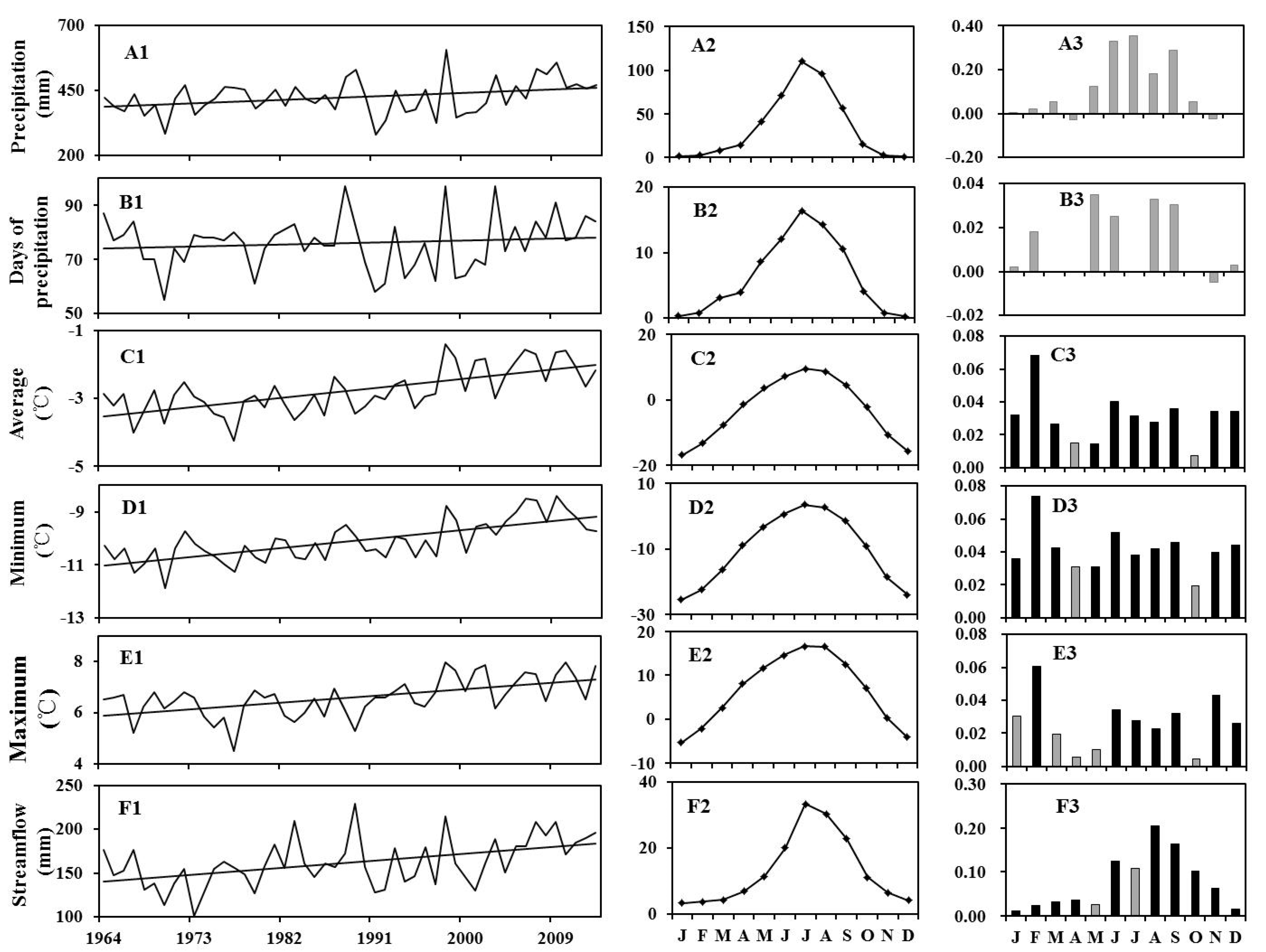
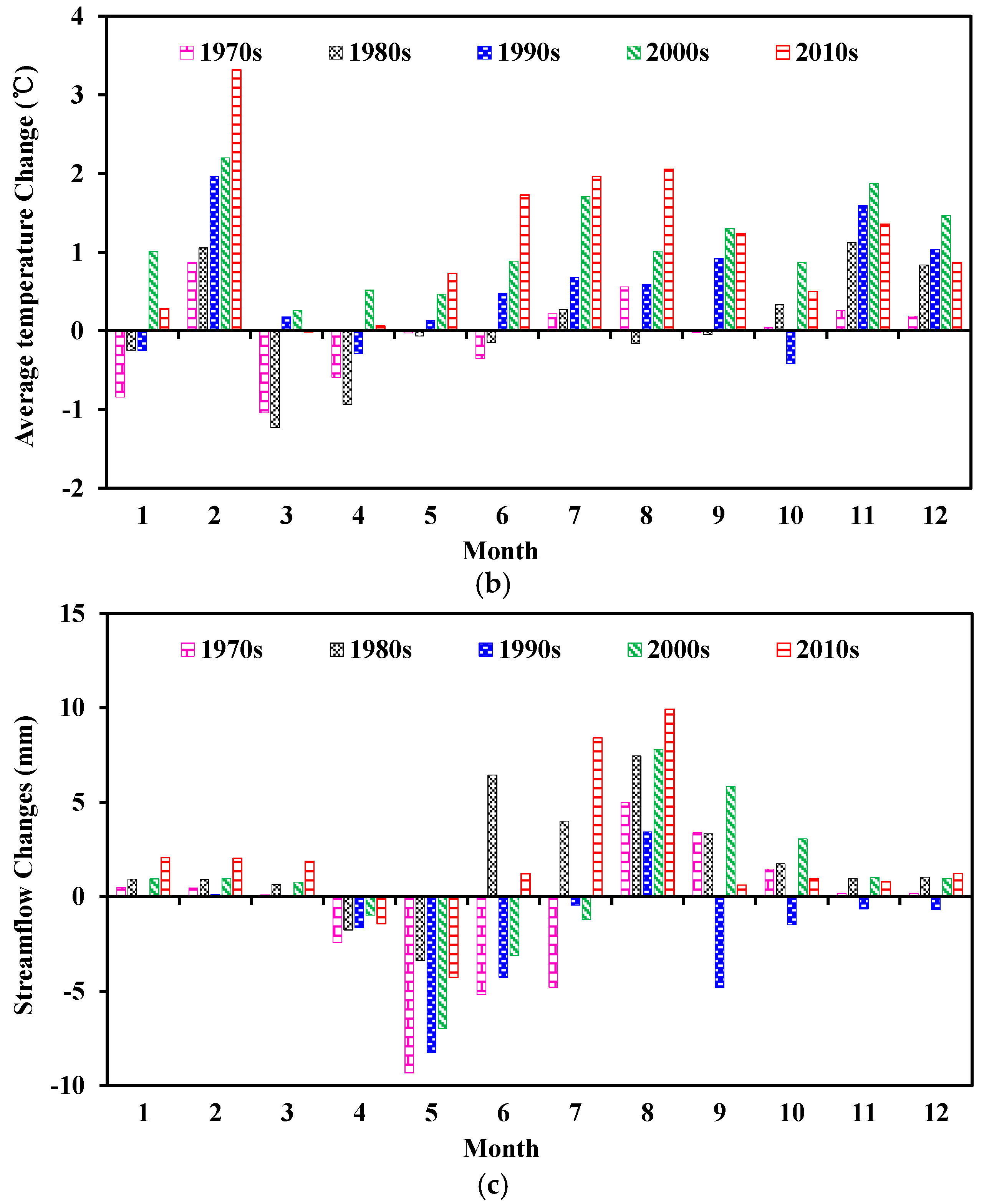
4.2. The Change in Hydro-Meteorological Variables
4.3. The Effects of Land Cover and Climate Change on Streamflow
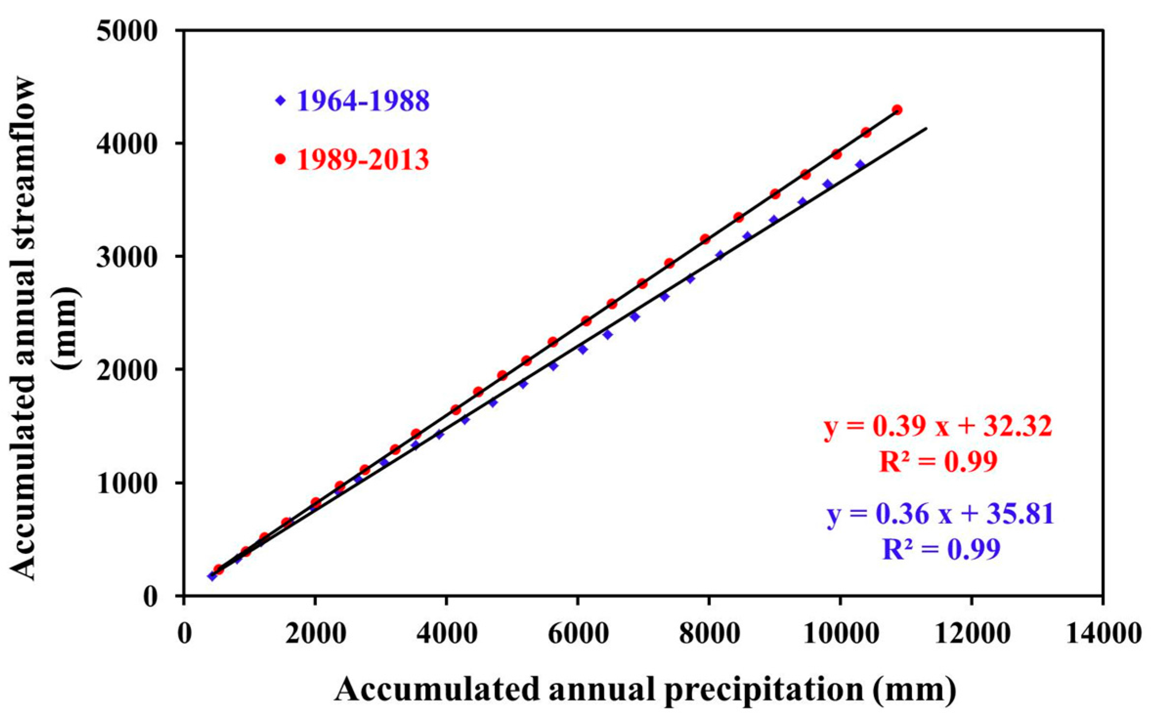
4.3.1. Identifing the Effects of Land Cover Change on Streamflow
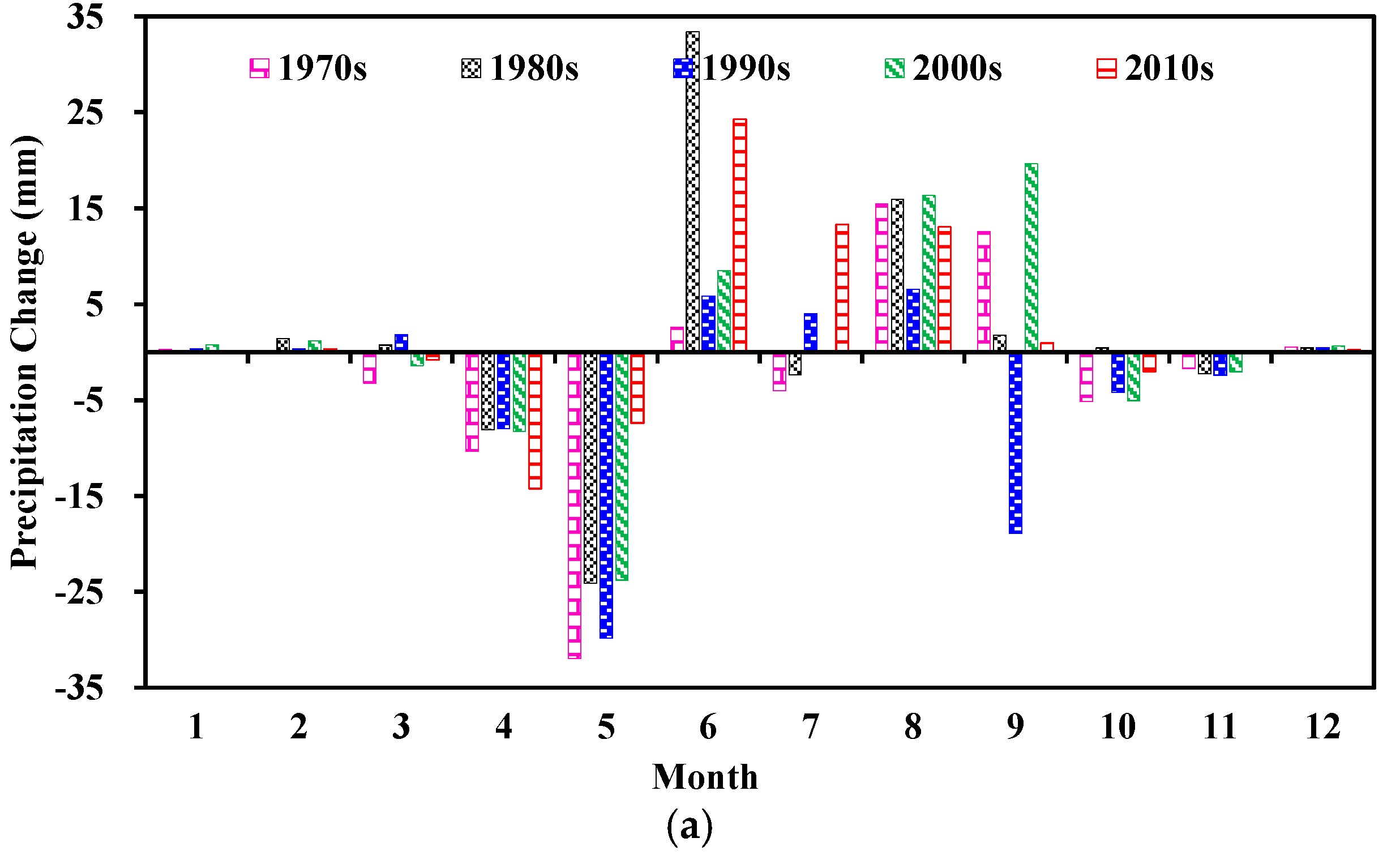
4.3.2. Quantifying Climate Change Contribution to Streamflow
5. Conclusions
Acknowledgments
Author Contributions
Conflicts of Interest
References
- Yang, D.; Gao, B.; Jiao, Y.; Lei, H.; Zhang, Y.; Yang, H.; Cong, Z. A distributed scheme developed for eco-hydrological modeling in the upper heihe river. Sci. China Earth Sci. 2014, 58, 36–45. [Google Scholar] [CrossRef]
- Feng, Q.; Miao, Z.; Li, Z.; Li, J.; Si, J.; S, Y.; Chang, Z. Public perception of an ecological rehabilitation project in inland river basins in northern China: Success or failure. Environ. Res. 2015, 139, 20–30. [Google Scholar] [CrossRef] [PubMed]
- Gao, G.; Fu, B.; Wang, S.; Liang, W.; Jiang, X. Determining the hydrological responses to climate variability and land use/cover change in the loess plateau with the budyko framework. Sci. Total Environ. 2016, 557–558, 331–342. [Google Scholar] [CrossRef] [PubMed]
- Milly, P.C.; Dunne, K.A.; Vecchia, A.V. Global pattern of trends in streamflow and water availability in a changing climate. Nature 2005, 438, 347–350. [Google Scholar] [CrossRef] [PubMed]
- Lopez-Moreno, J.I.; Zabalza, J.; Vicente-Serrano, S.M.; Revuelto, J.; Gilaberte, M.; Azorin-Molina, C.; Moran-Tejeda, E.; Garcia-Ruiz, J.M.; Tague, C. Impact of climate and land use change on water availability and reservoir management: Scenarios in the upper aragon river, Spanish pyrenees. Sci. Total Environ. 2014, 493, 1222–1231. [Google Scholar] [CrossRef] [PubMed]
- Ye, X.; Zhang, Q.; Liu, J.; Li, X.; Xu, C.-Y. Distinguishing the relative impacts of climate change and human activities on variation of streamflow in the poyang lake catchment, China. J. Hydrol. 2013, 494, 83–95. [Google Scholar] [CrossRef]
- Feng, Q.; Li, Z.; Liu, W.; Li, J.; Guo, X.; Wang, T. Relationship between large scale atmospheric circulation, temperature and precipitation in the extensive hexi region, China, 1960–2011. Quat. Int. 2016, 392, 187–196. [Google Scholar] [CrossRef]
- Gu, X.; Zhang, Q.; Singh, V.P.; Chen, Y.D.; Shi, P. Temporal clustering of floods and impacts of climate indices in the tarim river basin, China. Glob. Planet. Chang. 2016, 147, 12–24. [Google Scholar] [CrossRef]
- Tian, F.; Lü, Y.H.; Fu, B.J.; Yang, Y.H.; Qiu, G.; Zang, C.; Zhang, L. Effects of ecological engineering on water balance under two different vegetation scenarios in the Qilian mountain, northwestern China. J. Hydrol. Reg. Stud. 2016, 5, 324–335. [Google Scholar] [CrossRef]
- Ning, T.; Li, Z.; Liu, W. Separating the impacts of climate change and land surface alteration on runoff reduction in the Jing River catchment of China. Catena 2016, 147, 80–86. [Google Scholar] [CrossRef]
- Intergovernmental Panel on Climate Change. Climate Change 2013: The Physical Science Basis; IPCC: Cambridge, UK; New York, NY, USA, 2013. [Google Scholar]
- Ponpang-Nga, P.; Techamahasaranont, J. Effects of climate and land use changes on water balance in upstream in the Chao Phraya River Basin, Thailand. Agric. Nat. Resour. 2016, 50, 310–320. [Google Scholar] [CrossRef]
- Li, H.; Zhang, Y.; Vaze, J.; Wang, B. Separating effects of vegetation change and climate variability using hydrological modelling and sensitivity-based approaches. J. Hydrol. 2012, 420, 403–418. [Google Scholar] [CrossRef]
- Falkenmark, M.; Rockstrom, J. Balancing Water for Humans and Nature: The New Approach in Ecohydrology; Routledge: London, UK, 2004. [Google Scholar]
- DeFries, R.; Eshleman, K.N. Land-use change and hydrologic processes: A major focus for the future. Hydrol. Process. 2004, 18, 2183–2186. [Google Scholar] [CrossRef]
- Tomer, M.D.; Schilling, K.E. A simple approach to distinguish land-use and climate-change effects on watershed hydrology. J. Hydrol. 2009, 376, 24–33. [Google Scholar] [CrossRef]
- Zhang, L.; Nan, Z.; Yu, W.; Ge, Y. Modeling land-use and land-cover change and hydrological responses under consistent climate change scenarios in the Heihe River Basin, China. Water Resour. Manag. 2015, 29, 4701–4717. [Google Scholar] [CrossRef]
- Dessu, S.B.; Melesse, A.M. Modelling the rainfall-runoff process of the mara river basin using the soil and water assessment tool. Hydrol. Process. 2012, 26, 4038–4049. [Google Scholar] [CrossRef]
- Liu, Y.; Zhang, J.; Wang, G.; Liu, J.; He, R.; Wang, H.; Liu, C.; Jin, J. Quantifying uncertainty in catchment-scale runoff modeling under climate change (case of the Huaihe River, China). Quat. Int. 2012, 282, 130–136. [Google Scholar] [CrossRef]
- Qin, J.; Ding, Y.; Wu, J.; Gao, M.; Yi, S.; Zhao, C.; Ye, B.; Li, M.; Wang, S. Understanding the impact of mountain landscapes on water balance in the Upper Heihe River watershed in northwestern China. J. Arid Land 2013, 5, 366–383. [Google Scholar] [CrossRef]
- Xu, X.; Yang, D.; Yang, H.; Lei, H. Attribution analysis based on the budyko hypothesis for detecting the dominant cause of runoff decline in Haihe Basin. J. Hydrol. 2014, 510, 530–540. [Google Scholar] [CrossRef]
- Wang, X. Advances in separating effects of climate variability and human activity on stream discharge: An overview. Adv. Water Resour. 2014, 71, 209–218. [Google Scholar] [CrossRef]
- Zhao, A.; Zhu, X.; Liu, X.; Pan, Y.; Zuo, D. Impacts of land use change and climate variability on green and blue water resources in the Weihe River Basin of northwest China. Catena 2016, 137, 318–327. [Google Scholar] [CrossRef]
- Yan, R.; Gao, J.; Li, L. Modeling the hydrological effects of climate and land use/cover changes in Chinese lowland polder using an improved walrus model. Hydrol. Res. 2016, 47, 84–101. [Google Scholar] [CrossRef]
- Sarhadi, A.; Burn, D.H.; Johnson, F.; Mehrotra, R.; Sharma, A. Water resources climate change projections using supervised nonlinear and multivariate soft computing techniques. J. Hydrol. 2016, 536, 119–132. [Google Scholar] [CrossRef]
- Chiarelli, D.D.; Davis, K.F.; Rulli, M.C.; D’Odorico, P. Climate change and large-scale land acquisitions in africa: Quantifying the future impact on acquired water resources. Adv. Water Resour. 2016, 94, 231–237. [Google Scholar] [CrossRef]
- Zhang, L.; Podlasly, C.; Ren, Y.; Feger, K.-H.; Wang, Y.; Schwärzel, K. Separating the effects of changes in land management and climatic conditions on long-term streamflow trends analyzed for a small catchment in the loess plateau region, NW China. Hydrol. Process. 2014, 28, 1284–1293. [Google Scholar] [CrossRef]
- Lu, Z.; Zou, S.; Xiao, H.; Zheng, C.; Yin, Z.; Wang, W. Comprehensive hydrologic calibration of SWAT and water balance analysis in mountainous watersheds in northwest China. Phys. Chem. Earth Parts A/B/C 2015, 79–82, 76–85. [Google Scholar] [CrossRef]
- Geng, X.; Wang, X.; Yan, H.; Zhang, Q.; Jin, G. Land use/land cover change induced impacts on water supply service in the upper reach of Heihe River Basin. Sustainability 2014, 7, 366–383. [Google Scholar] [CrossRef]
- Huang, G. From water-constrained to water-driven sustainable development—A case of water policy impact evaluation. Sustainability 2015, 7, 8950–8964. [Google Scholar] [CrossRef]
- Yin, Z.; Feng, Q.; Zou, S.; Yang, L. Assessing variation in water balance components in Mountainous Inland River Basin experiencing climate change. Water 2016, 8, 472. [Google Scholar] [CrossRef]
- Wu, F.; Zhan, J.; Wang, Z.; Zhang, Q. Streamflow variation due to glacier melting and climate change in Upstream Heihe River Basin, northwest China. Phys. Chem. Earth Parts A/B/C 2015, 79–82, 11–19. [Google Scholar] [CrossRef]
- Zang, C.F.; Liu, J.; van der Velde, M.; Kraxner, F. Assessment of spatial and temporal patterns of green and blue water flows under natural conditions in Inland River Basins in northwest China. Hydrol. Earth Syst. Sci. 2012, 16, 2859–2870. [Google Scholar] [CrossRef] [Green Version]
- Deng, X.; Shi, Q.; Zhang, Q.; Shi, C.; Yin, F. Impacts of land use and land cover changes on surface energy and water balance in the Heihe River Basin of China, 2000–2010. Phys. Chem. Earth Parts A/B/C 2015, 79–82, 2–10. [Google Scholar] [CrossRef]
- Yin, Z.; Xiao, H.; Zou, S.; Zhu, R.; Lu, Z.; Lan, Y.; Shen, Y. Simulation of hydrological processes of mountainous watersheds in Inland River Basins: Taking the Heihe Mainstream River as an example. J. Arid Land 2013, 6, 16–26. [Google Scholar] [CrossRef]
- Yang, L.; Feng, Q.; Yin, Z.; Wen, X.; Si, J.; Li, C.; Deo, R.C. Identifying separate impacts of climate and land use/cover change on hydrological processes in Upper Stream of Heihe River, northwest China. Hydrol. Process. 2017, 31, 1100–1112. [Google Scholar] [CrossRef]
- Cheng, G.; Li, X.; Zhao, W.; Xu, Z.; Feng, Q.; Xiao, S.; Xiao, H. Integrated study of the water-ecosystem-economy in the Heihe River Basin. Natl. Sci. Rev. 2014, 1, 413–428. [Google Scholar] [CrossRef]
- Chen, Y.; Deng, H.; Li, B.; Li, Z.; Xu, C. Abrupt change of temperature and precipitation extremes in the arid region of northwest China. Quat. Int. 2014, 336, 35–43. [Google Scholar] [CrossRef]
- Li, B.; Chen, Y.; Shi, X. Why does the temperature rise faster in the arid region of northwest China? J. Geophys. Res. Atmos. 2012, 117, D16115. [Google Scholar] [CrossRef]
- Wang, H.; Chen, Y.; Xun, S.; Lai, D.; Fan, Y.; Li, Z. Changes in daily climate extremes in the arid area of northwestern China. Theor. Appl. Climatol. 2012, 112, 15–28. [Google Scholar] [CrossRef]
- Gao, Y.; Chen, F.; Barlage, M.; Liu, W.; Cheng, G.; Li, X.; Yu, Y.; Ran, Y.; Li, H.; Peng, H.; et al. Enhancement of land surface information and its impact on atmospheric modeling in the Heihe River Basin, northwest China. J. Geophys. Res. 2008, 113, D20S90. [Google Scholar] [CrossRef]
- Arnold, J.G.; Srinivasan, R.; Williams, J.R. Large area hydrologic modeling and assessment. Part I: Model development. J. Am. Water Resour. Assoc. 1998, 34, 73–89. [Google Scholar] [CrossRef]
- Neitsch, S.L.; Arnold, J.G.; Kiniry, J.R.; Williams, J.R. Soil and Water Assessment Tool Theoretical Documentation (Version 2005); USDA-ARS Grassland, Soil and Water Research Laboratory: Temple, TX, USA, 2005. [Google Scholar]
- Abbaspour, K.C. SWAT-CUP, SWAT Calibration and Uncertainty Programs; Swiss Federal Institute of Aquatic Science and Technology: Dübendorf, Switzerland, 2011. [Google Scholar]
- Moriasi, D.N.; Arnold, J.G.; Van Liew, M.W.; Bingner, R.L.; Harmel, R.D.; Veith, T.L. Model evaluation guidelines for systematic quantification of accuracy in watershed simulations. Trans. ASABE 2007, 50, 885–900. [Google Scholar] [CrossRef]
- Mann, H.B. Nonparametric tests against trend. Econometrica 1945, 13, 245–259. [Google Scholar] [CrossRef]
- Kendall, M.G. Rank Correlation Methods; Griffin: London, UK, 1975. [Google Scholar]
- Tesemma, Z.K.; Mohamed, Y.A.; Steenhuis, T.S. Trends in rainfall and runoff in the Blue Nile Basin: 1964–2003. Hydrol. Process. 2010, 24, 3747–3758. [Google Scholar] [CrossRef]
- Hamed, K.H. Trend detection in hydrologic data: The mann-kendall trend test under the scaling hypothesis. J. Hydrol. 2008, 349, 350–363. [Google Scholar] [CrossRef]
- Hamed, K.H.; Rao, A.R. A modified mann-kendall trend test for autocorrelated data. J. Hydrol. 1998, 204, 182–196. [Google Scholar] [CrossRef]
- Sen, P.K. Estimates of the regression coefficient based on kendall’s tau. J. Am. Stat. Assoc. 1968, 63, 1379–1389. [Google Scholar] [CrossRef]
- Wu, F.; Zhan, J.; Chen, J.; He, C.; Zhang, Q. Water yield variation due to forestry change in the head-water area of Heihe River Basin, northwest China. Adv. Meteorol. 2015, 2015, 1–8. [Google Scholar] [CrossRef]
- Wu, F.; Zhan, J.; Su, H.; Yan, H.; Ma, E. Scenario-based impact assessment of land use/cover and climate changes on watershed hydrology in Heihe River Basin of northwest China. Adv. Meteorol. 2015, 2015, 1–11. [Google Scholar] [CrossRef]


| Parameter 1 | Description | Parameter Range | Fitted Value |
|---|---|---|---|
| r_CN2.mgt | Initial SCS runoff curve number for moisture condition II | −0.4~0.2 | −0.225 |
| v_ALPHA_BF.gw | Base flow alpha factor (days) | 0.0~0.5 | 0.25 |
| v_GW_DELAY.gw | Groundwater delay time (days) | 90.0~180.0 | 165.0 |
| v_GWQMN.gw | Threshold depth of water in the shallow aquifer required for return flow to occur (mm) | 0.0~2.0 | 1.0 |
| v_GW_REVAP.gw | Groundwater ‘rewap’ coefficient | 0.0~0.2 | 0.033 |
| v_ESCO.hru | Soil evaporation compensation factor | 0.5~0.9 | 0.70 |
| v_CH_N2.rte | Manning’s ‘n’ value for the main channel | 0.0~0.3 | 0.05 |
| v_CH_K2.rte | Effective hydraulic conductivity in main channel alluvium (mm/h) | 5.0~40.0 | 10.83 |
| v_ALPHA_BNK.rte | Base flow alpha factor for bank storage | 0.0~1.0 | 0.50 |
| r_SOL_AWC.sol | Available water capacity of the soil layer (mm H2O/mm soil) | −0.2~0.4 | −0.10 |
| r_SOL_K.sol | Saturated hydraulic conductivity (mm/h) | −0.8~0.8 | −0.53 |
| v_SFTMP.bsn | Snowfall temperature (°C) | −2.0~1.0 | −1.5 |
| v_SMFMN.bsn | Melt factor on December 21 (mm H2O/°C-day) | 0~10.0 | 3.5 |
| v_SMFMX.bsn | Melt factor on June 21 (mm H2O/°C-day) | 0~10.0 | 7.5 |
| v_TLPAS.sub | Temperature lapse rate (°C/km) | −8.0~−4.0 | −5.5 |
| Period | NSE | R2 | PBIAS (%) |
|---|---|---|---|
| Calibration (1989–2000) | 0.93 | 0.95 | −3.47 |
| Validation (2001–2013) | 0.93 | 0.93 | 1.81 |
| The CV phase (1989–2013) | 0.93 | 0.93 | −0.59 |
| The IT phase (1964–1988) | 0.92 | 0.94 | 7.12 |
| Variable | Average | Slope of Regression Line (year−1) | M-K Test | β (year−1) | Significance |
|---|---|---|---|---|---|
| Precipitation (mm) | 420.65 | 1.542 | 2.52 | 1.487 | <0.05 |
| Days of precipitation (days) | 75.32 | 0.134 | 1.42 | 0.132 | - |
| Average air temperature (°C) | −2.83 | 0.030 | 4.82 | 0.030 | <0.01 |
| Minimum air temperature (°C) | −10.17 | 0.039 | 5.50 | 0.037 | <0.01 |
| Maximum air temperature (°C) | 6.58 | 0.026 | 3.84 | 0.027 | <0.01 |
| Streamflow (mm) | 160.28 | 0.914 | 3.92 | 0.937 | <0.01 |
| Decade | PCP (mm) | ta (°C) | R (mm) | PCP Change (mm) | ta Change (°C) | R Change (mm) | PCP (%) | ta (%) | R (%) |
|---|---|---|---|---|---|---|---|---|---|
| 1960s | 510.37 | −1.55 | 167.10 | - | - | - | - | - | - |
| 1970s | 499.47 | −1.66 | 153.54 | −10.90 | −0.11 | −13.56 | −2.14 | −7.10 | −8.11 |
| 1980s | 531.16 | −1.53 | 189.40 | 20.79 | 0.02 | 22.30 | 4.07 | 1.29 | 13.35 |
| 1990s | 498.02 | −1.05 | 151.44 | −12.35 | 0.50 | −15.66 | −2.42 | 32.26 | −9.39 |
| 2000s | 522.06 | −0.46 | 174.31 | 11.69 | 1.09 | 7.21 | 2.29 | 70.32 | 4.32 |
| 2010s | 528.21 | −0.42 | 190.50 | 17.84 | 1.13 | 23.40 | 3.50 | 72.90 | 14.01 |
© 2017 by the authors. Licensee MDPI, Basel, Switzerland. This article is an open access article distributed under the terms and conditions of the Creative Commons Attribution (CC BY) license (http://creativecommons.org/licenses/by/4.0/).
Share and Cite
Yin, Z.; Feng, Q.; Yang, L.; Wen, X.; Si, J.; Zou, S. Long Term Quantification of Climate and Land Cover Change Impacts on Streamflow in an Alpine River Catchment, Northwestern China. Sustainability 2017, 9, 1278. https://doi.org/10.3390/su9071278
Yin Z, Feng Q, Yang L, Wen X, Si J, Zou S. Long Term Quantification of Climate and Land Cover Change Impacts on Streamflow in an Alpine River Catchment, Northwestern China. Sustainability. 2017; 9(7):1278. https://doi.org/10.3390/su9071278
Chicago/Turabian StyleYin, Zhenliang, Qi Feng, Linshan Yang, Xiaohu Wen, Jianhua Si, and Songbing Zou. 2017. "Long Term Quantification of Climate and Land Cover Change Impacts on Streamflow in an Alpine River Catchment, Northwestern China" Sustainability 9, no. 7: 1278. https://doi.org/10.3390/su9071278