Association between Three-Dimensional Built Environment and Urban Air Temperature: Seasonal and Temporal Differences


Department of Urban Planning and Engineering, Hanyang University, Seoul 04763, Korea
*
Author to whom correspondence should be addressed.
Sustainability 2017, 9(8), 1338; https://doi.org/10.3390/su9081338
Submission received: 1 June 2017
/
Revised: 26 July 2017
/
Accepted: 26 July 2017
/
Published: 31 July 2017
(This article belongs to the Section Sustainable Urban and Rural Development)
Abstract
:Climate change and the urban heat island phenomenon are increasingly important issues in urban thermal environments. However, there is a lack of research on the relationship between three-dimensional built environments and air temperature. Therefore, the purpose of this study is to provide policy suggestions that could be used to improve urban thermal environments by analyzing the effect of the three-dimensional built environment of an urban space on the urban air temperature according to changes in time (i.e., season, time of day). Using data from 236 automatic weather stations (AWSs) in Seoul, Korea, this study focused on three-dimensional built environmental variables and land use variables that affect air temperature in terms of season and time. The analysis results indicate that the sky view factor and porosity were lower in urban areas, with higher sky view factor and porosity values associated with lower air temperature. This study also indicates that surface roughness is higher in urban areas, with higher surface roughness associated with higher air temperature. These results suggest that urban design practices should consider the three-dimensional built environment when planning urban development and urban regeneration projects in order to improve the urban thermal environment.
1. Introduction
Recently, researchers and policy makers have become interested in mitigation strategies to combat the urban heat island effect and global warming. The characteristics of built environments in urban areas have substantial effects on the urban thermal environment. In particular, the urban heat island effect during the summer is a main threat to the daily lives of urban residents. The consistent and severe heat problems in the summer of 2016 in Korea called public attention to the necessity of mitigation strategies for the urban heat island effect. The high temperature caused by the urban heat island effect during the summer months is an urgent issue that should be dealt with because it increases heat-related illnesses such as heat exhaustion and stroke.
Previous studies suggest that high temperature in the city center is associated with high-density development, large number of impervious surfaces, few green areas, and air pollution [1,2,3,4,5]. However, in Hong Kong, the air temperature of the city center was lower than that of the sub-center due to the ventilation effect and the smaller amount of solar radiation [6,7]. This result indicates that increasing the building density does not necessarily increase the air temperature in urban areas. Instead, the three-dimensional characteristics of the urban environment can affect the air temperature in a complicated way.
The purpose of this study is to analyze the effect of the three-dimensional built environment on urban air temperature in Seoul. This study examines the relationship between the three-dimensional built environment and urban air temperature as a function of time (i.e., season, time of day). To analyze the built environment factors that affect the air temperature, we applied both two- and three-dimensional built environmental characteristics of urban space including the sky view factor, surface roughness, and porosity level.
2. Literature Review
Several studies have analyzed the relationships between two-dimensional urban characteristics and the thermal environment [1,2,3,4,5,8,9]. In particular, previous studies have examined the mitigation effect of green space on urban temperature. In studies employing satellite images, such as Landsat data, an increased green space ratio was observed with a decrease in air temperature [10,11]. In addition, it was also reported that a single large green space or a number of smaller green spaces could cause a cool island effect, thereby reducing the air temperature [12]. Previous studies have indicated that the mitigation effect of green space varies according to its density, size, and shape [13,14,15].
Another factor that affects air temperature is albedo, which is the reflection ratio of solar radiation. An area with a high albedo level was observed to show a lower surface temperature [16]. The albedo level is highly related with the materials of roofing sheets or road surfaces [17]. Land use was also reported to be a significant factor that affects the urban temperature, especially in areas where human activities increase at night [18]. Furthermore, anthropogenic heat, including the heat from traffic, human activities, and major facilities, was observed to be an important determinant of the urban thermal environment [19,20]. In a study analyzing 47 areas in South Korea, an increase in traffic showed a high association with an increase in urban temperature [21].
Urban areas that have undergone high-density development with high-rise buildings are more likely to experience an increase in urban air temperature. Therefore, researchers have developed three-dimensional measures such as the sky view factor, roughness, and porosity that can quantify the urban environment [22,23,24,25]. For instance, a higher sky view factor, which indicates a high ratio of sky visibility at a certain point, decreases the urban temperature. The mitigation effect of the sky view factor can be explained through the canyon effect, which is more likely to decrease the air circulation in areas with lower sky view factor, leading to higher air temperature [26]. Generally, the sky view factor is lower in areas with many high-rise buildings [24]. In addition, an increase in sky view factor decreases the urban air temperature during both the day and night [25].
The roughness of an urban area is used to estimate the arrangement of buildings and open spaces. A lower surface roughness can cause higher wind speeds and form wind pathways that can lower urban temperature and heat stress [27]. Like surface roughness, roughness length can also be used to estimate wind speed and wind path in urban areas [28,29]. Since cool wind from suburban areas or green spaces can decrease urban temperature, the wind path is an important factor for mitigating urban heat islands [30]. On the other hand, porosity, which is the ratio of vacant space, is a significant index for urban street canyons. Low porosity can disturb ventilation in high-rise building areas, increase urban temperature, and lower pedestrian-level thermal comfort [31,32].
Regarding the effects of three-dimensional urban factors on air temperature, Chun & Guldmann showed that a higher sky view factor leads to lower urban temperature [33]. On the other hand, Theeuwes et al. analyzed the seasonal effect of aspect ratio on urban temperature [34]. According to their results, the effect of aspect ratio on air temperature differed by season. The seasonal difference in the effect of aspect ratio on air temperature was attributed to the changes in solar radiation levels. Most recently, Chun and Guhathakurta examined the effect of three-dimensional urban factors on the urban heat island, focusing on its variation over the day and night [35]. They reported that tall buildings can mitigate the surface temperature during the daytime because of their shadows, but can also create an urban heat island at night because of the low sky view factor.
However, urban areas with high-rise buildings do not necessarily experience increased urban air temperature due to the influx of daytime solar radiation, which is a critical factor influencing urban air temperature during the daytime. As a result, several studies analyzing the relationship between sky view factor and air temperature for both day and night have reported slightly different results [24,25,33,35]. These differences are attributed to the different number of samples, study area, and other weather factors such as wind and humidity. In addition, few studies have analyzed how buildings, roads, and open spaces interact with solar radiation and wind [6,7,36].
Furthermore, few studies have attempted to analyze the seasonal effects of urban factors on air temperature [34,37,38,39]. For instance, Hamada and Ohta reported that the effect of green open space on air temperature differs by season [39]. In addition, Taleghani et al. showed that green open space continuously mitigates the urban air temperature during both the summer and winter [37]. These results are attributed to changes in vegetation level and climate factors including wind and humidity. Thus, the determinant factors of the urban heat island and air temperature have been widely examined for two-or three-dimensional urban features. In addition, the effects of urban features have been analyzed while considering both the temporal and seasonal effects.
However, the shortcomings of previous studies are as follows. First, only a few studies have examined the relationship between the three-dimensional built environment and the urban air temperature. The three-dimensional characteristics including sky view factor, surface roughness, and porosity are factors that can be used to effectively describe the built environment. They are also intimately related to the solar radiation and wind tunnel effects. Second, most previous studies focused on urban air temperature in summer. Summer is a crucial season for examining the determinants of urban air temperature; however, since Korea has four distinct seasons, it is necessary to analyze the urban air temperature for other seasons as well. Furthermore, it is necessary to analyze whether the built environmental variables show a consistent effect on urban air temperature throughout all four seasons. Third, few studies have examined the relationship between air temperature and the three-dimensional built environment during both the day and night. Since solar radiation directly affects the thermal environment only during the day, it is necessary to analyze both time periods within a day. Lastly, previous studies investigating the urban thermal environment are limited due to the lack of high-resolution urban temperature data. For instance, most of the studies focused on Seoul were based on a small amount of automatic weather station (AWS) data. Therefore, it can be difficult to generalize the analysis results and conclusions.
Based on the shortcomings of previous studies, the novelty of this study is as follows. First, we examined the relationship between the three-dimensional built environment and the urban air temperature using an extensive amount of urban air temperature data. We analyzed the air temperature in Seoul using the observation data of 236 AWSs, including AWSs operated by the Korean Meteorological Administration (KMA) and SK Weather Planet (SKWP). Second, in addition to two-dimensional factors, we considered three-dimensional built environment variables of sky view factor, surface roughness, and porosity. Third, we investigated the effects of built environment characteristics on the urban thermal environment as a function of season. The urban thermal conditions are important for all four seasons because they are linked to issues such as energy consumption and air pollution. It is especially important to manage the cool island effect during the winter. Finally, we analyzed the determinants of air temperature for both the daytime and nighttime while considering the influence of solar radiation.
3. Research Measures and Methodology
3.1. Study Area
The study area for this project was Seoul, the capital city of South Korea. Seoul is located at 37.6 latitude and 127.0 longitude and has a total area of approximately 605 . The population is about 9.9 million with a population density of 16.3 thousand people per . In 2015, the annual mean temperature was 13.6 °C, and the highest and lowest temperatures were 36.0 °C and −13.0 °C, respectively. The Han River (6.9% of the Seoul city area), which crosses the city from east to west, and the mountainous areas (24.5% of the Seoul city area) located in the north and south highlight the three-dimensional characteristics of the urban environment (see Figure 1).
3.2. Description of Variables
This study classifies independent variables into four groups: weather characteristics and altitude, two-dimensional built environment, land use, and three-dimensional built environment. The weather characteristics and altitude factors are wind speed, solar radiation, and altitude of the AWS. The wind speed was used to examine the influence of wind intensity on urban air temperature. In general, higher wind speeds are known to lower the air temperature by circulating air within an area [21,40]. The solar radiation affects the weather conditions, and its value is also influenced by the three-dimensional built environment. In addition, we considered the altitude of the AWSs because the 236 AWSs utilized in our study are located in the city center as well as in the peripheral mountain areas.
For the two-dimensional built environment, we used surface albedo, green space, road area, building area, and gross floor area. Surface albedo indicates the ratio of the reflection level of the surface. As albedo increases, the solar radiation at the surface decreases, which leads to mitigation of air temperature [16]. Green areas also lower the urban air temperature by forming cold islands [12]. Tree evapotranspiration reduces the air temperature, with the shade areas formed by trees reducing the surface temperature by as much as 6–8 °C in the summer [10,41]. In contrast, road area, which has low heat capacity and low albedo, increases the air temperature. Building area and gross floor area were used to consider the development density of the area.
For land use variables, we considered the total floor area of residential, commercial, and office building uses. The floor area according to building use is used to estimate the occurrence of anthropogenic heat caused by human activity and facility utilization. Commercial areas can generate more anthropogenic heat from people and facilities than other areas during the daytime.
For the three-dimensional built environment variables, this study uses the sky view factor, surface roughness, and porosity. First, the sky view factor indicates the ratio of visible sky at a certain point, reflecting the characteristics of high-density urban areas [24,25,42]. The sky view factor is measured as a value between 0.0 and 1.0. A higher sky view factor enhances the ventilation effect, resulting in a lower urban air temperature. Next, the surface roughness, which focuses on the height and distribution of buildings, was used to analyze the effects of three-dimensional characteristics on air temperature. The roughness length index could have been used as a similar index; however, we applied the surface roughness index because it is easier to calculate and more intuitive. We expected that an increase in surface roughness would result in an increase in urban air temperature. Finally, the porosity represents the volume ratio of empty space and is computed by excluding the volume of buildings in the urban canyon. When the porosity value is high, a higher ventilation effect and a lower air temperature are expected.
3.3. Methods for Computing Variables
This study used 500 m buffer areas around the AWS installation sites as the unit of analysis for analyzing the neighboring areas based on the locations of the AWSs. Therefore, the independent variables of the built environment were measured within a 500-m buffer.
3.3.1. Air Temperature and Wind Speed
This study used air temperature data measured from 236 AWSs, including 27 Korean Meteorological Administration AWSs and 209 SK Weather Planet AWSs. The AWS data also included wind speed. We excluded the days when rainfall or snowfall exceeded 5 mm in order to control instant changes in weather conditions caused by rainfall or snowfall. To analyze the seasonal variation of air temperature determinants, we defined April, August, October, and January as spring, summer, fall, and winter, respectively. In addition, we divided the data based on the sunrise and sunset times to analyze the temporal variation for both daytime and nighttime (see Table 1). According to the time period in Table 1, the air temperature and the wind speed were averaged over each period.
3.3.2. Solar Radiation and Altitude
The amount of solar radiation directly increases air temperature, as well as surface temperature, based on the amount of energy emitted by the sun onto the surface or building. For example, the highest daytime temperature occurs between 12 and 14 o’clock because the sun is located in the highest position during this time and the solar radiation is the strongest. Moreover, the criteria used for distinguishing daytime from nighttime were the sunrise and sunset times, which indicate the presence or absence of solar radiation.
The amount of solar radiation was computed using the ArcGIS program, with the elevation and building data of Seoul used as the input data sources. Because there is no direct solar radiation at night, we did not consider solar radiation as a variable in the nighttime model. For altitude, the average altitude value of the 500 m buffer area of each AWS location was applied using the Seoul Digital Elevation Model (DEM).
3.3.3. Two-Dimensional Built Environment
First, surface albedo was calculated using Landsat 8 data from the USGS. For analyzing the entire area of Seoul, the 2015 Landsat image with the least cloud cover was used. Smith suggested a method to calculate albedo from Landsat 7 data, which we used by adjusting the new band number of Landsat 8 data [43]. Also, the New Address Database of the Ministry of Government Administration and Home Affairs including the geographic information system (GIS) shape data was used to calculate the other two-dimensional built environment variables.
3.3.4. Land Use
In order to measure the total area for each type of building use, the building ledge database was applied. The building register data contain the type of use, area, floor, and address. To use this information for spatial analysis with other data in ArcGIS, we transformed the building register data into spatial data via geocoding analysis. To represent anthropogenic heat from human activity and facility operation in the case study area, this study aggregated the floor area of each land use of residential, commercial, and office use.
3.3.5. Sky View Factor
The sky view factor indicates the ratio of visible sky from a certain observation point. More specifically, it indicates the ratio of the open sky space in the hemisphere formed toward the center from an observation point [44,45]. The numerical range for the sky view factor is from 0 to 1. In general, a larger value means more open space where the air circulation is smoother. Furthermore, it is known that the sky view factor is intimately related with solar radiation.
Most previous studies that have dealt with the sky view factor utilized fisheye lenses or GIS to measure the value. Using a fisheye lens enables the sky view factor to be calculated accurately by considering the concrete forms of buildings and plants. However, since this method requires that a photograph be taken during a field survey, there are difficulties in collecting data for many locations. In addition, measuring the sky view factor with a fisheye lens in our study was not viable because we examined the determinants of air temperature seasonally. Therefore, we measured the sky view factor using the ArcGIS program. A variety of studies have suggested programs (e.g., ArcView SVF Extension, SOLWEIG, and SkyHelios) for calculating the sky view factor and have reported that the results are highly correlated with the values measured using a fisheye lens [21,45].
In this study, we used the ‘skyline’ and ‘skyline graph’ functions in ArcGIS 10 to compute the sky view factor. First, the ‘skyline’ function constructs spatial information about the basic boundary, which is necessary to compute the sky view factor at a certain observation point. Next, the ‘skyline graph’ function computes the sky view factor based on the ‘skyline’ results (see Figure 2). This methodology requires information about the observation point where the sky view factor is being measured as well as the 3D spatial information of the analysis site. In this study, we used the average value of the sky view factor calculated within the 500 m buffer of each AWS location to explain the air temperature. This method was first suggested by Chen et al. [24], who reported that the areal sky view factor is appropriate when analyzing air temperature. In addition, the points for computing the sky view factor were selected within a 500 m buffer area of each AWS location. After plotting the observation points with a grid spacing of 50 m, points on the road or the ground were finally selected as the observation points (see Figure 3).
3.3.6. Surface Roughness
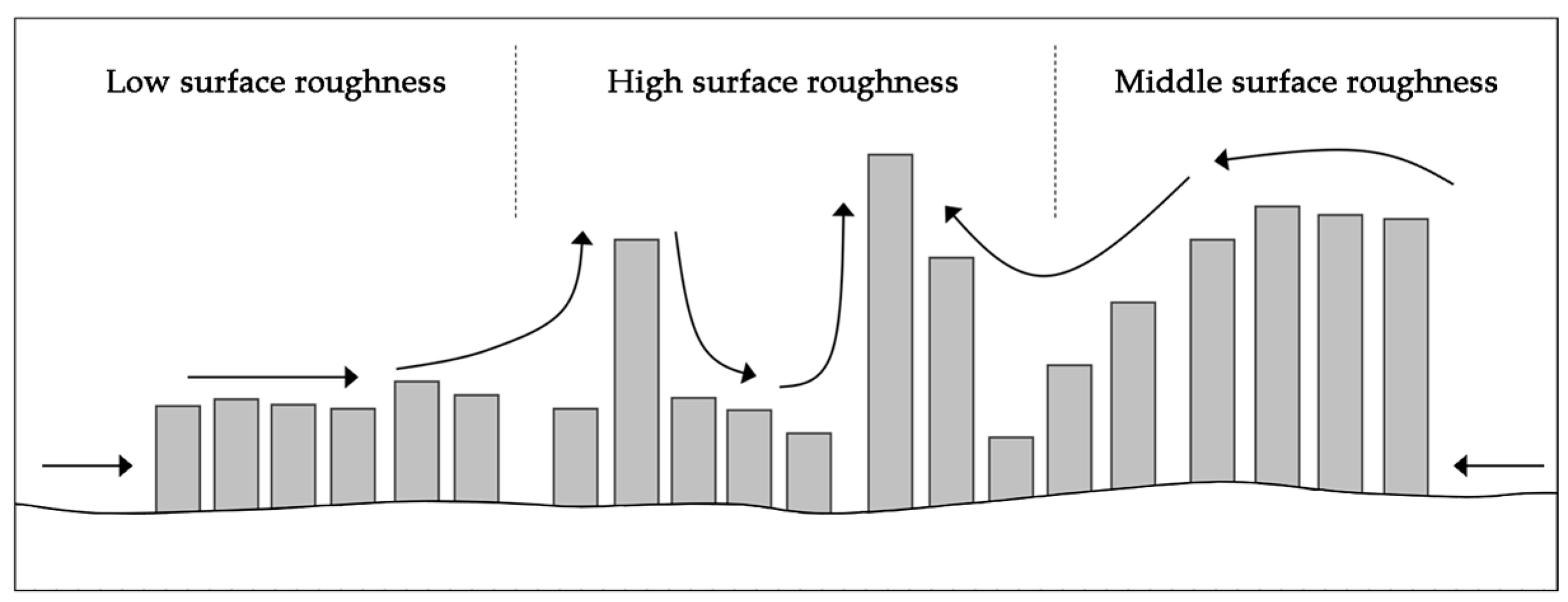
Surface roughness refers to the irregularity of the three-dimensional shape of an area. In particular, it is related to the degree of irregularity of buildings. Generally, a higher surface roughness value leads to less wind circulation, which results in an increase in air temperature. In previous studies [27,28], either the standard deviation of building height or the concept of roughness length was typically used to measure the surface roughness parameter.
In this study, we used the standard deviation of building height as the variable for surface roughness. This method is intuitive and requires relatively simple computing processes. To measure this variable, grids with a unit of 5 m were created for the 500 m buffer area around each station. The height was then measured from the center point of each grid. The surface roughness represents the irregularity of the building heights and is highly correlated with air temperature. When the surface roughness is low, the wind circulation is expected to be high, resulting in a decrease in urban air temperature. In contrast, if the surface roughness is high, as shown in the middle of Figure 4, the wind circulation is expected to be low, which can negatively affect urban air temperature.
3.3.7. Porosity
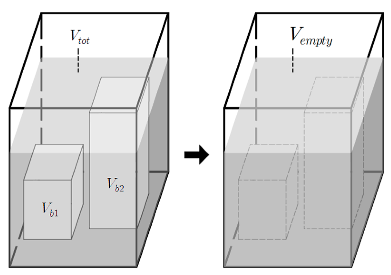
Porosity generally refers to the ratio of void space within a total volume of space. The porosity of a city indicates the volume ratio of the void space excluding buildings and artificial structures (see Figure 5). Moreover, porosity expresses the empty space between urban canyons. Porosity is highly related with the formation of wind pathways, and it is reported that higher porosity values enhance wind circulation, thereby lowering the air temperature.
Gál and Unger [28] proposed two methods for calculating porosity. The two methods differ in how they select the maximum height used to calculate the total volume (Vtotal) of the analysis site. The first method designates the maximum height as the height of the top of the city, including the floor and buildings. Alternatively, the second method uses the maximum height of the building floor within each analysis unit. For Seoul, the difference in elevation between AWS sites is large because there are many mountainous areas. Therefore, if porosity is calculated according to the first method, there will be under- or overestimation issues. Thus, we employed the second method to measure the porosity value.
3.4. Research Process and Methodology
To examine the changes in the effects of independent variables on the seasonal air temperature, we used air temperatures in January, April, August, and October to represent winter, spring, summer, and autumn, respectively. In addition, we divided the air temperature data into daytime and nighttime to consider solar radiation. First, we analyzed the descriptive statistics to observe the seasonal differences in urban air temperature and weather characteristics. In addition, we examined other variables including the three-dimensional built environment and the land use characteristics. Second, we analyzed the correlation between urban air temperature and each independent variable. Finally, we examined the effects of the independent variables on urban air temperature using the multiple regression model. Table 2 shows the variables applied in this study.
4. Analysis Results and Interpretations
4.1. Descriptive Analysis
The descriptive statistics of the variables are shown in Table 3. The descriptive statistics of air temperature, wind speed, and solar radiation are presented by season. As seen in Table 3, the average daytime air temperatures in spring, summer, autumn, and winter were 15.6 °C, 27.8 °C, 17.9 °C, and 1.0 °C, respectively. Alternatively, the average nighttime air temperatures of the four seasons were 12.5 °C, 25.2 °C, 14.7 °C, and −0.9 °C, respectively. Moreover, regardless of the season, the gap between the maximum and minimum values was about 4–6 °C. Also, for the standard deviation of air temperature, the highest values for daytime and nighttime were observed in the summer and autumn, respectively. For wind speed, spring showed the highest wind speed among the four seasons, and the average value was always higher in the daytime than in the nighttime. The average value of solar radiation was in descending order of summer, spring, autumn, and winter.
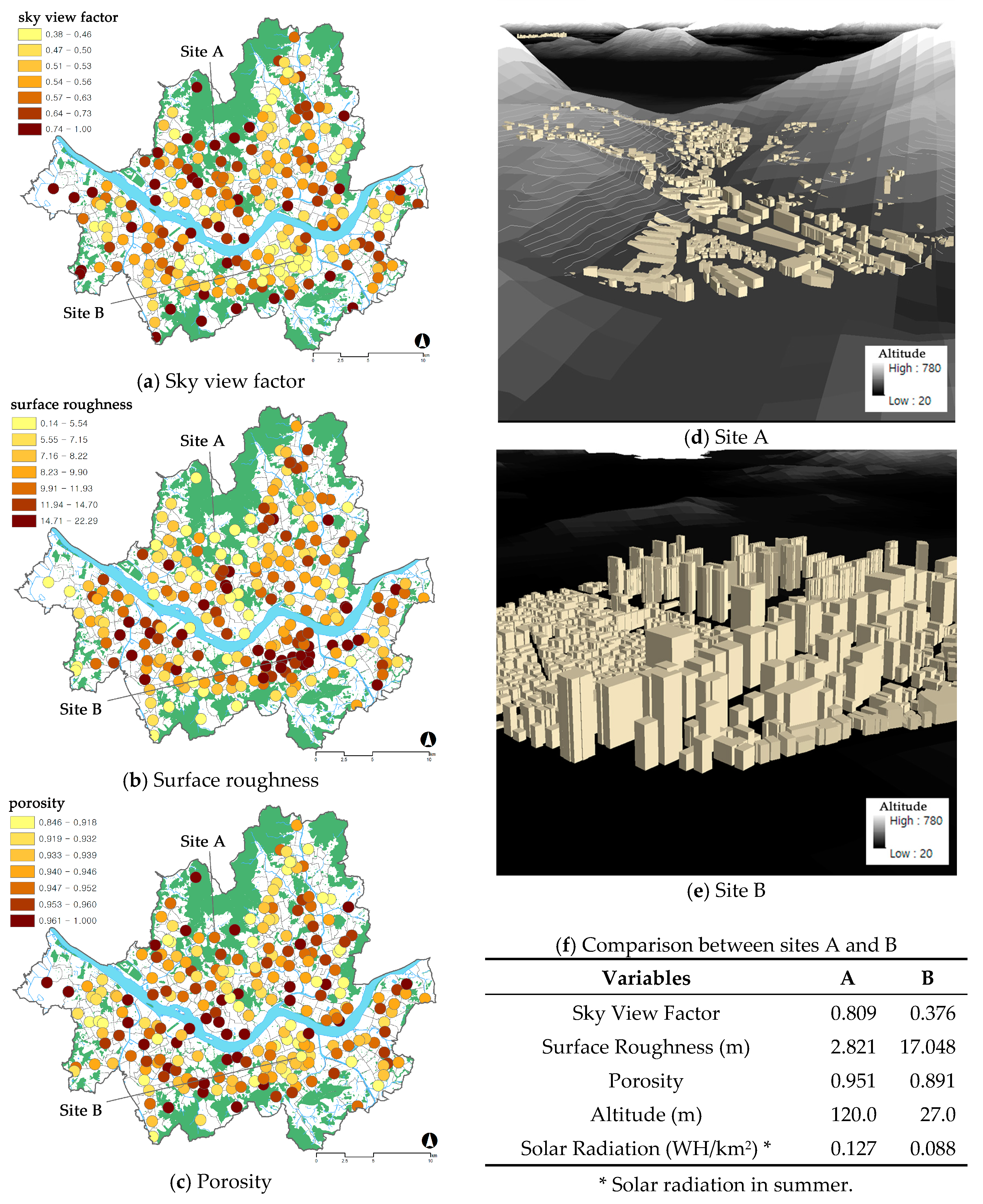
For the three-dimensional built environment variables, the average sky view factor was 0.58, while the sky view factor value varied from 0.38 to 0.99. The average surface roughness was 9.74, with minimum and maximum values of 0.14 and 22.29, respectively. The average porosity was 0.94, and varied from 0.85 to 0.99. For the AWS sites in mountainous areas, including the areas of Bukhan Mountain and Gwanak Mountain, the sky view factor and porosity value were both close to 1.00, and the surface roughness was lowest (Site A in Figure 6). In contrast, the AWS sites with low sky view factors, low porosity, and high surface roughness were mainly found in the central business districts such as in the Gangnam area (Site B in Figure 6).
For land use variables, the average of the gross floor area was in ascending order of residential, commercial, and office uses. In addition, the gross floor area of office buildings showed the highest standard deviation, implying that office buildings are concentrated in only a few areas. In the case of green spaces, the average green space area in the 500 m buffer areas was approximately 0.075 .
4.2. Correlation Analysis Results
4.2.1. Correlation Analysis with Air Temperature
The results of the correlation analysis between air temperature and the independent variables are shown in Table 4. The air temperature was divided by season and time (day or night). The wind speed only showed a significantly negative correlation with the daytime air temperature, regardless of season. Alternatively, altitude showed a negative correlation with air temperature regardless of season and time. For solar radiation, a negative correlation with air temperature was observed. However, this does not imply that higher solar radiation reduces air temperature because the solar radiation itself is influenced by the physical environment of the site. The amount of solar radiation influx within a 500 m buffer area around the AWS location was lower in the high-rise urban areas than in the mountainous areas (see Figure 6f). This is due to the shade created by the high-rise buildings, which results in less solar radiation at the ground level.
Albedo and green space showed negative correlations with urban air temperature, indicating that high albedo and increase in green space could reduce urban air temperature. On the contrary, road area, building area, and gross floor area had positive correlations with air temperature. Among the land use variables, all variables showed positive correlations, while commercial use showed the highest correlation with urban air temperature. This means that land use can differently affect urban air temperature according to the land use type.
In the case of the three-dimensional built environments, the sky view factor and porosity showed negative correlations with urban air temperature. In contrast, surface roughness showed a positive correlation with air temperature. Green space showed a negative correlation with air temperature, while the gross floor areas of residential, commercial, or office uses showed positive correlations. In summary, the results of the correlation analysis showed that the three-dimensional built environment variables had a significant correlation with air temperature regardless of season or time. In addition, the land use variables also showed expected results (i.e., positive associations with residential, commercial, or office uses and a negative association with green space).
4.2.2. Correlation Analysis between Independent Variables
To understand the relationships among independent variables, this study conducted correlation analyses (see Table 5). First, among the three-dimensional built environmental variables, surface roughness was the only variable with a significant correlation with wind speed. For solar radiation, gross floor area and sky view factor showed high correlations over 0.8. Interestingly, sky view factor showed a high correlation with building area, but surface roughness had a low correlation under 0.2. However, surface roughness had a high correlation with gross floor area, over 0.8.
4.3. Results of Multiple Regression Analysis
Table 6 and Table 7 show the results of eight multiple regression models as a function of season and time. This study excluded road area, building area, and gross floor area variables based on the correlation analysis and multicollinearity test. In addition, albedo was not included in the daytime model due to a multicollinearity problem with solar radiation. Wind speed showed a significant relationship with daytime air temperature for all seasons but only in the spring nighttime. The coefficients indicated that higher wind speed lowers the air temperature. The coefficient of wind speed was highest in summer, implying that wind speed critically affects summer air temperature. Solar radiation showed a significant relationship with air temperature only in summer and autumn. Moreover, the coefficient of solar radiation was positive, which is different from the results obtained via correlation analysis. This discrepancy is caused by our consideration of other important variables of the AWS site in the multiple regression models. Finally, altitude showed a significant and negative relationship with air temperature throughout the seasons and times.
Regardless of season, albedo and green space showed significant negative effects at night. Because two-dimensional built environment variables have cooling effects at night, the surface temperature is likely to have a strong impact on the urban thermal condition after sunset. From the perspective of the seasonal effect, the two-dimensional built environmental variables showed a higher impact on urban air temperature in autumn and winter. Thus, when applying albedo and green space to improve urban thermal environment, we should consider the seasonal effects.
The results of the land use variables are as follows. First, residential GFA did not show a significant association with air temperature. However, commercial GFA showed a significant and positive relationship with air temperature in the nighttime of all seasons and in the daytime of summer and autumn. In contrast, in the case of office GFA, there was a significant and negative association with air temperature during the nighttime of summer and autumn, as well as during the daytime of autumn. These results indicate the effects of human and facility activities on air temperature because other built environments were considered. In other words, for commercial GFA, there were activities that raised the nighttime air temperature regardless of season. In addition, the different coefficient values of commercial and office GFAs can be caused by differences in the activities of humans and facilities.
The three-dimensional built environments showed statistically significant results for different seasons and times. First, the sky view factor showed a negative relationship with air temperature in the nighttime of spring, summer, and autumn, as well as in the daytime of summer. Thus, the sky view factor is an effective measure for cooling urban heat in summer. Next, the surface roughness showed a significant and positive relationship with air temperature during the nighttime of all seasons, with the highest coefficient observed in autumn. Lastly, porosity showed a significant and negative relationship with air temperature only in the daytime of summer, autumn, and winter.
5. Conclusions
This study analyzed the impact of three-dimensional built environments on air temperature as a function of season and time. The main results of this analysis are as follows.
First, the three-dimensional built environment variables of sky view factor, surface roughness, and porosity showed statistically significant associations with air temperature. The sky view factor was lower in urban centers (e.g., Gangnam) and higher in peripheral mountainous areas. Regression analysis showed that a higher sky view factor generally lowers the urban air temperature. Surface roughness showed a positive association with nighttime air temperature during all seasons. The increased surface roughness, due to the large structures and high-rise buildings, showed a negative relationship with air temperature because wind flow was reduced. Additionally, porosity showed a significant and positive relationship with daytime air temperature due to the ventilation effect when porosity level is high. The analysis results also indicated that the impact of the three-dimensional built environment on air temperature was higher in the summer than in the winter. Thus, three-dimensional built environment variables can be used as effective indicators for urban design strategies for the mitigation of summer heatwaves and their side effects.
Second, daytime wind speeds were higher than those during the nighttime, and the regression analysis showed that higher wind speed reduces the air temperature throughout all four seasons. Since the wind intensity is influenced by the physical environment of the site, the importance of designing a ‘wind path’ is significant when attempting to improve the urban thermal environment.
Third, the level of solar radiation was higher in summer and spring and showed a significant relationship with air temperature. The regression analysis results indicated that higher solar radiation showed a positive relationship with higher urban air temperature. While urban centers receive less solar radiation due to the shade provided by high-rise buildings, these areas show higher air temperature due to the high-density development and concentrated human activities.
Fourth, land use showed a significant relationship with air temperature based on correlation and multiple regression analyses. Commercial GFA showed a positive relationship with nighttime air temperature, indicating that most of the urban activities after sunset are concentrated in commercial areas. In contrast, office GFA showed a negative relationship with air temperature, implying a reduction in urban activities in office areas after sunset. The amount of green space showed a negative relationship with urban air temperature. Since green spaces can cause a cool island effect, which decreases urban heat, this indicates the need to include green spaces and/or urban parks to improve urban thermal comfort.
In conclusion, this study suggests the following policy implications. First, we should consider three-dimensional built environment variables, such as the sky view factor, surface roughness and porosity, during urban planning and urban design practices in order to improve urban thermal comfort. Second, a wind path is necessary to enhance the function of air ventilation in urban spaces. A wind path can lower air temperatures in urban centers during the summer and also reduce air pollution. Third, two-dimensional built environment variables such as albedo and green spaces should be actively applied to reduce urban air temperature in city centers.
However, despite the important findings of this study, these results might not be generalizable because we only used air temperature data from 2015. In addition, we were unable to account for a few variables in the regression model due to multi-collinearity. Therefore, future studies should consider air temperature data for multiple years and attempt an analysis that can deal with the variables excluded in our analysis.
Acknowledgments
This work was supported by a Korean Agency for Infrastructure Technology Advancement (KAIA) grant funded by the Ministry of Land, Infrastructure, and Transport (Grant 17AUDP-B102406-03).
Author Contributions
As the lead author, Cheolyeong Park initiated this study with an original idea and conducted the overall analysis. He also wrote an initial draft of the manuscript based on his master’s thesis at Hanyang University. Jaehyun Ha, as a co-author, assisted data analysis and developed the manuscript. Sugie Lee, as a corresponding author, developed the original idea of this study and suggested appropriate methodologies for the overall analysis. All authors have read, provided feedback on, and approved the final manuscript.
Conflicts of Interest
The authors declare no conflict of interest.
References
- Lowry, W.P. Weather and Life: An Introduction to Biometeorology; Academic Press: Cambridge, MA, USA, 1969. [Google Scholar]
- Oke, T.R. City size and the urban heat island. Atmos. Environ. 1973, 7, 769–779. [Google Scholar] [CrossRef]
- Park, H.S. Features of the heat island in Seoul and its surrounding cities. Atmos. Environ. 1986, 20, 1859–1866. [Google Scholar] [CrossRef]
- Lee, H.Y. A study on urban heat islands over the metropolitan Seoul area, using satellite images. J. Korean Geogr. Soc. 1989, 24, 1–13. [Google Scholar]
- He, J.F.; Liu, J.Y.; Zhuang, D.F.; Zhang, W.; Liu, M.L. Assessing the effect of land use/land cover change on the change of urban heat island intensity. Theor. Appl. Climatol. 2007, 90, 217–226. [Google Scholar] [CrossRef]
- Giridharan, R.; Lau, S.S.Y.; Ganesan, S.; Givoni, B. Urban design factors influencing heat island intensity in high-rise high-density environments of Hong Kong. Build. Environ. 2007, 42, 3669–3684. [Google Scholar] [CrossRef]
- Giridharan, R.; Lau, S.S.Y.; Ganesan, S.; Givoni, B. Lowering the outdoor temperature in high-rise high-density residential developments of coastal Hong Kong: The vegetation influence. Build. Environ. 2008, 43, 1583–1595. [Google Scholar] [CrossRef]
- Mackey, C.W.; Lee, X.; Smith, R.B. Remotely sensing the cooling effects of city scale efforts to reduce urban heat island. Build. Environ. 2012, 49, 348–358. [Google Scholar] [CrossRef]
- Lin, W.; Yu, T.; Chang, X.; Wu, W.; Zhang, Y. Calculating cooling extents of green parks using remote sensing: Method and test. Landsc. Urban Plan. 2015, 134, 66–75. [Google Scholar] [CrossRef]
- Oh, K.S.; Hong, J.J. The relationship between urban spatial elements and the urban heat island effect. J. Korean Urban Des. 2015, 18, 47–63. [Google Scholar]
- Yun, H.C.; Kim, M.G.; Jung, K.Y. Analysis of temperature change by forest growth for mitigation of the urban heat island. J. Korean Soc. Surv. 2013, 31, 143–150. [Google Scholar] [CrossRef]
- Kong, F.; Yin, H.; James, P.; Hutyra, L.R.; He, H.S. Effects of spatial pattern of greenspace on urban cooling in a large metropolitan area of eastern China. Landsc. Urban Plan. 2014, 128, 35–47. [Google Scholar] [CrossRef]
- Feyisa, G.L.; Dons, K.; Meilby, H. Efficiency of parks in mitigating urban heat island effect: An example from Addis Ababa. Landsc. Urban Plan. 2014, 123, 87–95. [Google Scholar] [CrossRef]
- Fintikakis, N.; Gaitani, N.; Santamouris, M.; Assimakopoulos, M.; Assimakopoulos, D.N.; Fintikaki, M.; Albanis, G.; Papadimitriou, K.; Chryssochoides, E.; Katopodi, K.; et al. Bioclimatic design of open public spaces in the historic centre of Tirana, Albania. Sustain. Cities Soc. 2011, 1, 54–62. [Google Scholar] [CrossRef]
- Lehmann, I.; Mathey, J.; Rößler, S.; Bräuer, A.; Goldberg, V. Urban vegetation structure types as a methodological approach for identifying ecosystem services: Application to the analysis of micro-climatic effects. Ecol. Indic. 2014, 42, 58–72. [Google Scholar] [CrossRef]
- Jeong, J.J. Comparison of land surface temperatures derived from surface emissivity with urban heat island effect. J. Environ. Impact Assess. Assoc. Korea 2009, 18, 219–227. [Google Scholar]
- Yuan, J.; Emura, K.; Farnham, C. Highly reflective roofing sheets installed on a school building to mitigate the urban heat island effect in Osaka. Sustainability 2016, 8, 514. [Google Scholar] [CrossRef]
- Song, B.G.; Park, K.H. Analysis of heat island characteristics considering urban space at nighttime. J. Korean Assoc. Geogr. Inf. Stud. 2012, 15, 133–143. [Google Scholar] [CrossRef]
- Grimmond, C.S.B.; Christen, A. Flux measurements in urban ecosystems. FluxLett. Newsl. FLUXNET 2012, 5, 1–7. [Google Scholar]
- Lindberg, F.; Grimmond, C.S.B.; Yogeswaran, N.; Kotthaus, S.; Allen, L. Impact of city changes and weather on anthropogenic heat flux in Europe 1995–2015. Urban Clim. 2013, 4, 1–15. [Google Scholar] [CrossRef]
- Cho, H.S.; Jeong, Y.J.; Choi, M.J. Effects of the urban spatial characteristics on urban heat island. J. Korea Environ. Policy Adm. Soc. 2014, 22, 27–43. [Google Scholar] [CrossRef]
- Svensson, M.K. Sky view factor analysis-implications for urban air temperature differences. Meteorol. Appl. 2004, 11, 201–211. [Google Scholar] [CrossRef]
- Unger, J. Connection between urban heat island and sky view factor approximated by a software tool on a 3D urban database. Int. J. Environ. Pollut. 2008, 36, 59–80. [Google Scholar] [CrossRef]
- Chen, L.; Ng, E.; An, X.; Ren, C.; Lee, M.; Wang, U.; He, Z. Sky view factor analysis of street canyons and its implications for daytime intra-urban air temperature differentials in high-rise, high-density urban areas of Hong Kong: A GIS-based simulation approach. Int. J. Climatol. 2012, 32, 121–136. [Google Scholar] [CrossRef]
- Ha, J.; Lee, S.; Park, C. Temporal effects of environmental characteristics on urban air temperature: The influence of the sky view factor. Sustainability 2016, 8, 895. [Google Scholar] [CrossRef]
- Nunez, M.; Oke, T.R. The energy balance of an urban canyon. J. Appl. Meteorol. 1977, 16, 11–19. [Google Scholar] [CrossRef]
- Ng, E.; Yuan, C.; Chen, L.; Ren, C.; Fung, J.C. Improving the wind environment in high-density cities by understanding urban morphology and surface roughness: a study in Hong Kong. Landsc. Urban Plan. 2011, 101, 59–74. [Google Scholar] [CrossRef]
- Gál, T.; Unger, J. Detection of ventilation paths using high-resolution roughness parameter mapping in a large urban area. Build. Environ. 2009, 44, 198–206. [Google Scholar] [CrossRef]
- An, S.M.; Lee, K.S.; Yi, C.Y. Building wind corridor network using roughness length. J. Korean Inst. Landsc. Arch. 2015, 169, 101–113. [Google Scholar] [CrossRef]
- Song, Y.B. The Plan and Design for Wind Path; Green Tomato: Seoul, Korea, 2007. [Google Scholar]
- Chun, B.S.; Kim, H.Y. Analysis of urban heat island effect using information from 3-dimensional city model. J. Korea Spat. Inf. Soc. 2010, 18, 1–11. [Google Scholar]
- Yuan, C.; Ng, E. Building porosity for better urban ventilation in high-density cities-A computational parametric study. Build. Environ. 2012, 50, 176–189. [Google Scholar] [CrossRef]
- Chun, B.; Guldmann, J.M. Spatial statistical analysis and simulation of the urban heat island in high-density central cities. Landsc. Urban Plan. 2014, 125, 76–88. [Google Scholar] [CrossRef]
- Theeuwes, N.E.; Steeneveld, G.J.; Ronda, R.J.; Heusinkveld, B.G.; Van Hove, L.W.A.; Holtslag, A.A.M. Seasonal dependence of the urban heat island on the street canyon aspect ratio. Q. J. R. Meteorol. Soc. 2014, 140, 2197–2210. [Google Scholar] [CrossRef]
- Chun, B.; Guhathakurta, S. The impacts of three-dimensional surface characteristics on urban heat islands over the diurnal cycle. Prof. Geogr. 2017, 69, 191–202. [Google Scholar] [CrossRef]
- Takebayashi, H.; Moriyama, M. Relationships between the properties of an urban street canyon and its radiant environment: Introduction of appropriate urban heat island mitigation technologies. Sol. Energy 2012, 86, 2255–2262. [Google Scholar] [CrossRef]
- Taleghani, M.; Tenpierik, M.; Van Den Dobbelsteen, A.; Sailor, D.J. Heat mitigation strategies in winter and summer: Field measurements in temperate climates. Build. Environ. 2014, 81, 309–319. [Google Scholar] [CrossRef]
- Wang, Y.; Akbari, H. Analysis of urban heat island phenomenon and mitigation solutions evaluation for Montreal. Sustain. Cities Soc. 2016, 26, 438–446. [Google Scholar] [CrossRef]
- Hamada, S.; Ohta, T. Seasonal variations in the cooling effect of urban green areas on surrounding urban areas. Urban For. Urban Green. 2010, 9, 15–24. [Google Scholar] [CrossRef]
- Kim, Y.J.; Kang, D.H.; Ahn, K.H. Characteristics of urban heat-island phenomena caused by climate changes in Seoul, and alternative urban design approaches for their improvements. J. Urban Des. Inst. Korea 2011, 12, 5–14. [Google Scholar]
- Lee, E.Y.; Moon, S.K.; Shim, S.R. A study on the effect of air temperature and ground temperature mitigation from several arrangements of urban green. J. Korean Inst. Landsc. Arch. 1996, 24, 65–78. [Google Scholar]
- An, S.M.; Kim, B.S.; Lee, H.Y.; Kim, C.H.; Yi, C.Y.; Eum, J.H.; Woo, J.H. Three-dimensional point cloud based sky view factor analysis in complex urban settings. Int. J. Climatol. 2014, 34, 2685–2701. [Google Scholar] [CrossRef]
- Smith, R.B. The Heat Budget of the Earth’s Surface Deduced from Space; Yale University Center for Earth Observation: New Haven, CT, USA, 2010. [Google Scholar]
- Oke, T.R. Canyon geometry and the nocturnal urban heat island: Comparison of scale model and field observations. J. Climatol. 1981, 1, 237–254. [Google Scholar] [CrossRef]
- Hämmerle, M.; Gál, T.; Unger, J.; Matzarakis, A. Comparison of models calculating the sky view factor used for urban climate investigations. Theor. Appl. Climatol. 2011, 105, 521–527. [Google Scholar] [CrossRef]
Figure 1.
Study area and the 236 AWSs in Seoul, Korea.
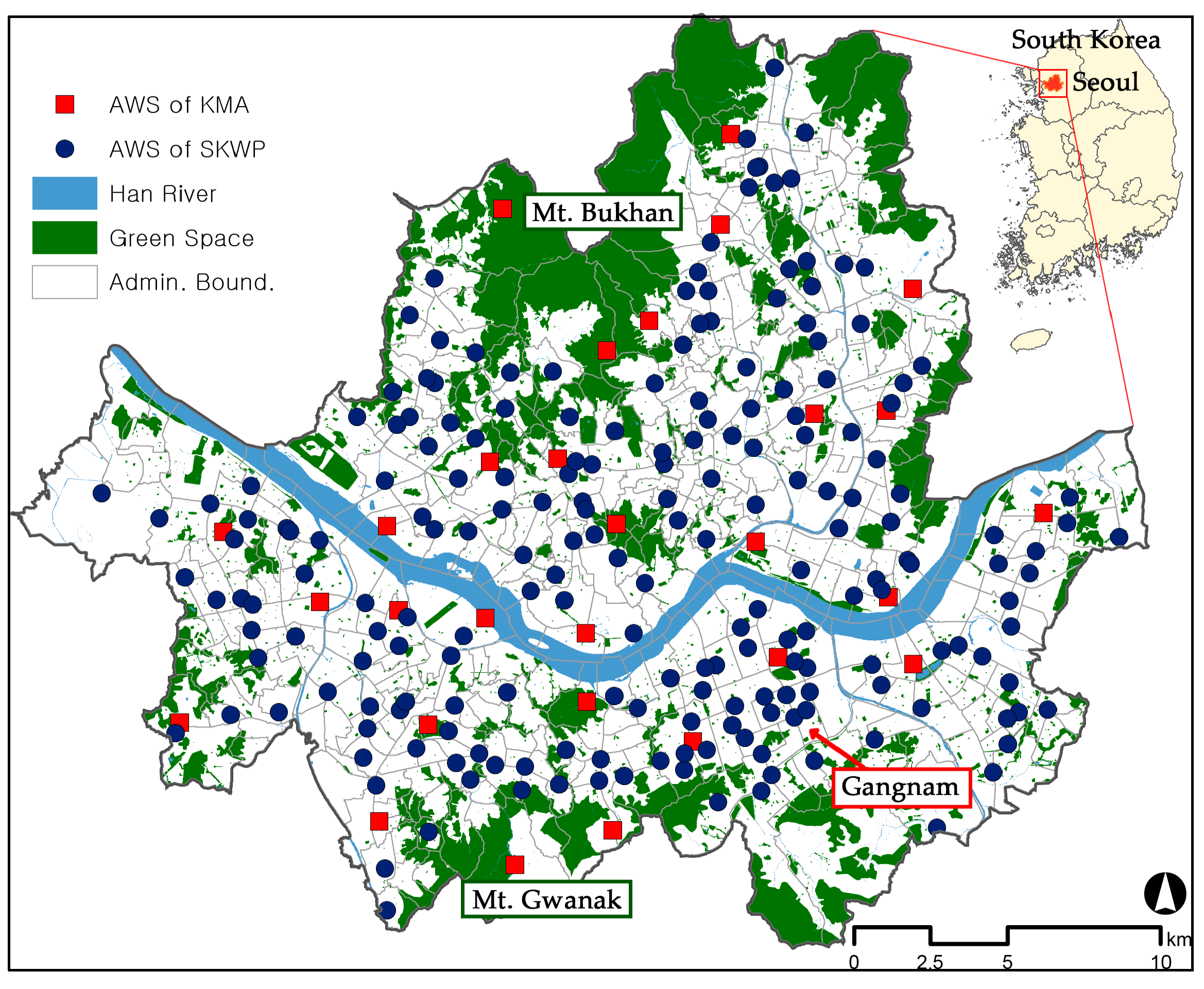
Figure 2.
Skyline graph and sky view factor calculation in ArcGIS.
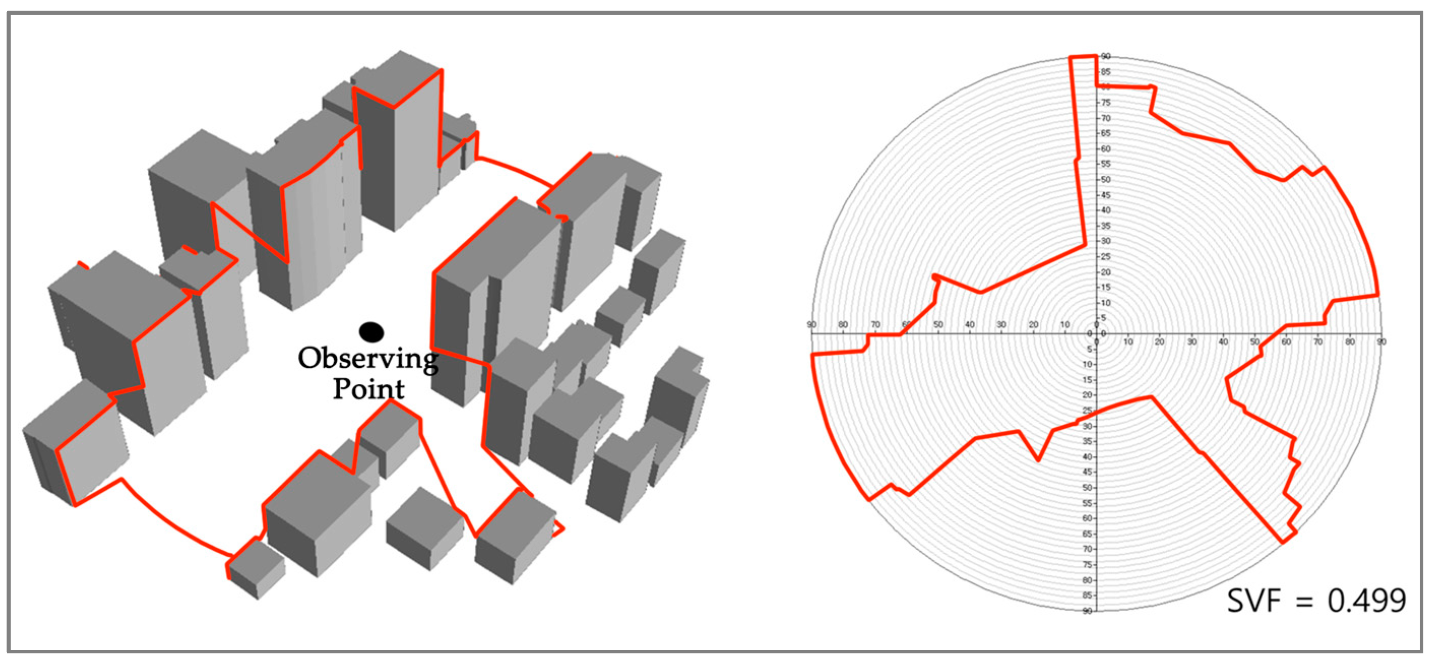
Figure 3.
Selection process of the observation points for sky view factor. (Source: Adapted from [25])
Figure 3.
Selection process of the observation points for sky view factor. (Source: Adapted from [25])
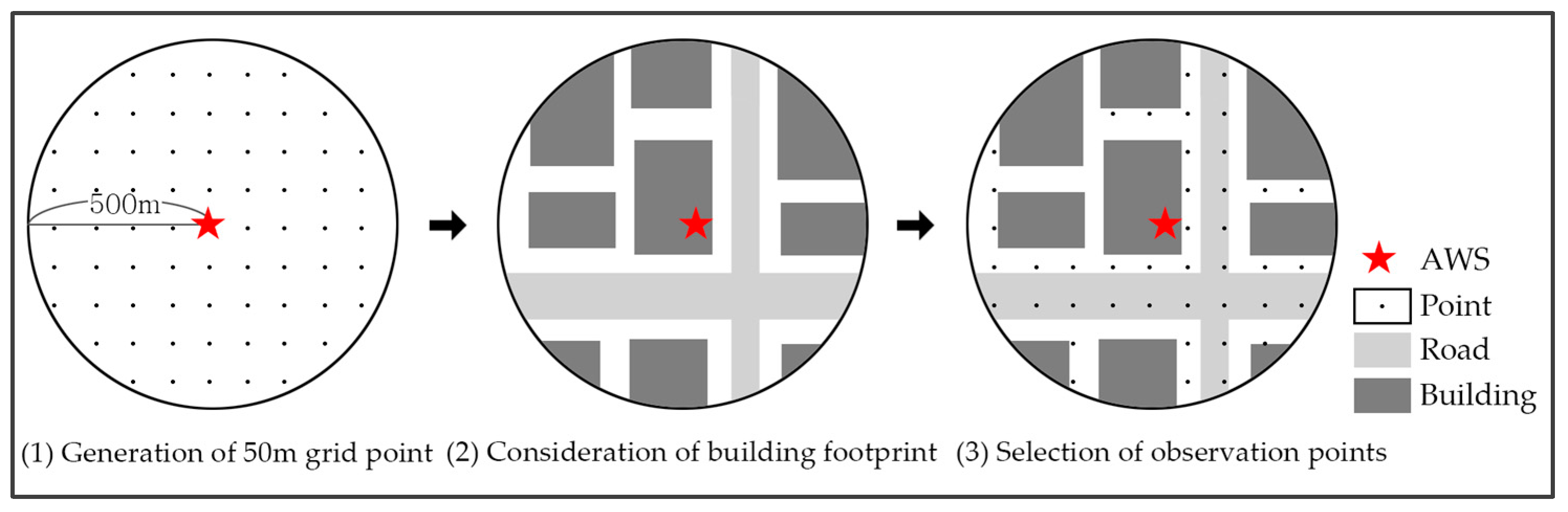
Figure 4.
Surface roughness in urban areas.

Figure 5.
Concept of porosity.

Figure 6.
Three-dimensional built environments around selected AWSs.

Table 1.
Sunrise and sunset times for the different seasons. Source: Korea Astronomy Observatory.
| Season | Date | Sunrise | Sunset | Daytime | Nighttime |
|---|---|---|---|---|---|
| Spring | 04.01 | 6:19 | 18:54 | 7a.m.–18p.m. | 20p.m.–5a.m. |
| 04.30 | 5:39 | 19:20 | |||
| Summer | 08.01 | 5:35 | 19:41 | 7a.m.–18p.m. | 20p.m.–5a.m. |
| 08.31 | 6:01 | 19:04 | |||
| Autumn | 10.01 | 6:27 | 18:16 | 8a.m.–17p.m. | 19p.m.–6a.m. |
| 10.31 | 6:55 | 17:36 | |||
| Winter | 01.01 | 7:47 | 17:24 | 9a.m.–17p.m. | 19p.m.–7a.m. |
| 01.31 | 7:37 | 17:54 |
Table 2.
Variable description.
| Variable | Unit | Description | |
|---|---|---|---|
| Air Temperature | °C | Average temperature in daytime and nighttime | |
| Weather Characteristics and Altitude | Wind Speed | m/s | Average wind speed in daytime and nighttime |
| Solar Radiation | WH/km2 | Average solar radiation within the 500 m buffer | |
| Altitude | M | Average altitude within the 500 m buffer | |
| Two-Dimensional Built Environment | Albedo | - | Average surface albedo within the 500 m buffer |
| Green Space | Km2 | Area of green space within the 500 m buffer | |
| Road Area | Km2 | Area of roads within the 500 m buffer | |
| Building Area | Km2 | Area of buildings within the 500 m buffer | |
| Gross Floor Area (GFA) | km2 | Gross floor area within the 500 m buffer | |
| Land Use | Residential Use | km2 | Gross floor area of residential use within the 500 m buffer |
| Commercial Use | km2 | Gross floor area of commercial use within the 500 m buffer | |
| Office Use | km2 | Gross floor area of office use within the 500 m buffer | |
| Three-Dimensional Built Environment | Sky View Factor | - | Average sky view factor calculated in a 50 m × 50 m grid within the 500 m buffer |
| Surface Roughness | m | Standard deviation of height in a 5 m × 5 m grid within the 500 m buffer | |
| Porosity | - | Ratio of vacant space, excluding buildings and structures, within the 500 m buffer | |
Table 3.
Descriptive statistics.
| Variable | Unit | Avg. | Std. Dev. | Min. | Max. | |||
|---|---|---|---|---|---|---|---|---|
| Air Temperature | Spring | Day | °C | 15.557 | 0.436 | 13.306 | 17.485 | |
| Night | °C | 12.509 | 0.724 | 9.042 | 14.727 | |||
| Summer | Day | °C | 27.841 | 0.497 | 24.918 | 29.762 | ||
| Night | °C | 25.219 | 0.691 | 22.125 | 26.838 | |||
| Autumn | Day | °C | 17.875 | 0.459 | 15.263 | 19.302 | ||
| Night | °C | 14.713 | 0.868 | 10.312 | 16.304 | |||
| Winter | Day | °C | 0.964 | 0.428 | −1.857 | 2.093 | ||
| Night | °C | −0.893 | 0.664 | −4.437 | 0.733 | |||
| Weather Characteristics and Altitude | Wind Speed | Spring | Day | m/s | 2.285 | 0.573 | 0.615 | 4.204 |
| Night | m/s | 1.547 | 0.509 | 0.361 | 4.018 | |||
| Summer | Day | m/s | 1.998 | 0.513 | 0.568 | 4.053 | ||
| Night | m/s | 1.578 | 0.510 | 0.383 | 3.677 | |||
| Autumn | Day | m/s | 2.022 | 0.532 | 0.613 | 4.170 | ||
| Night | m/s | 1.426 | 0.491 | 0.259 | 3.369 | |||
| Winter | Day | m/s | 2.109 | 0.567 | 0.666 | 3.787 | ||
| Night | m/s | 1.698 | 0.550 | 0.367 | 3.747 | |||
| Solar Radiation | Spring | WH/km2 | 0.102 | 0.010 | 0.077 | 0.132 | ||
| Summer | WH/km2 | 0.115 | 0.010 | 0.088 | 0.147 | |||
| Autumn | WH/km2 | 0.052 | 0.006 | 0.036 | 0.071 | |||
| Winter | WH/km2 | 0.026 | 0.004 | 0.017 | 0.037 | |||
| Altitude | m | 37.435 | 25.747 | 20.000 | 253.081 | |||
| Two-Dimensional Built Environment | Albedo | - | 0.128 | 0.008 | 0.106 | 0.166 | ||
| Green Space | 0.075 | 0.120 | 0.000 | 0.784 | ||||
| Road Area | 0.160 | 0.050 | 0.000 | 0.265 | ||||
| Building Area | 0.211 | 0.073 | 0.000 | 0.347 | ||||
| Gross floor Area | 1.074 | 0.487 | 0.001 | 2.718 | ||||
| Land Use | Residential Use | 0.591 | 0.301 | 0.000 | 1.699 | |||
| Commercial Use | 0.254 | 0.198 | 0.000 | 1.140 | ||||
| Office Use | 0.143 | 0.297 | 0.000 | 2.179 | ||||
| Three-Dimensional Built Environment | Sky View Factor | - | 0.583 | 0.133 | 0.376 | 0.997 | ||
| Surface Roughness | m | 9.691 | 4.448 | 0.144 | 22.287 | |||
| Porosity | - | 0.940 | 0.023 | 0.846 | 1.000 | |||
Table 4.
Correlation analysis with air temperature.
| Variables | Daytime | Nighttime | |||||||
|---|---|---|---|---|---|---|---|---|---|
| Spring | Summer | Autumn | Winter | Spring | Summer | Autumn | Winter | ||
| Weather Characteristics and Altitude | Wind Speed | −0.450 *** | −0.263 *** | −0.318 *** | −0.341 *** | 0.105 | 0.080 | 0.084 | 0.090 |
| Solar Radiation | −0.260 *** | −0.240 *** | −0.158 ** | −0.241 *** | - | - | - | - | |
| Altitude | −0.334 *** | −0.413 *** | −0.403 *** | −0.514 *** | −0.477 *** | −0.541 *** | −0.450 *** | −0.506 *** | |
| Two-Dimensional Built Environment | Albedo | −0.127 * | −0.102 | −0.049 | −0.057 | −0.282 *** | −0.207 *** | −0.283 *** | −0.297 *** |
| Green Space | −0.186 *** | −0.303 *** | −0.255 *** | −0.348 *** | −0.500 *** | −0.511 *** | −0.469 *** | −0.509 *** | |
| Road Area | 0.187 *** | 0.292 *** | 0.251 *** | 0.331 *** | 0.563 *** | 0.541 *** | 0.559 *** | 0.556 *** | |
| Building Area | 0.174 *** | 0.250 *** | 0.214 *** | 0.234 *** | 0.503 *** | 0.474 *** | 0.475 *** | 0.450 *** | |
| Gross Floor Area | 0.309 *** | 0.291 *** | 0.214 *** | 0.281 *** | 0.546 *** | 0.471 *** | 0.487 *** | 0.503 *** | |
| Land Use | Residential Use | 0.163 ** | 0.163 ** | 0.146 ** | 0.187 *** | 0.368 *** | 0.318 *** | 0.306 *** | 0.321 *** |
| Commercial Use | 0.256 *** | 0.281 *** | 0.224 *** | 0.242 *** | 0.452 *** | 0.409 *** | 0.441 *** | 0.437 *** | |
| Office Use | 0.205 *** | 0.126 * | 0.041 | 0.086 | 0.240 *** | 0.168 ** | 0.193 *** | 0.221 *** | |
| Three-Dimensional Built Environment | Sky View Factor | −0.267 *** | −0.301 *** | −0.226 *** | −0.288 *** | −0.602 *** | −0.544 *** | −0.526 *** | −0.531 *** |
| Surface Roughness | 0.309 *** | 0.281 *** | 0.220 *** | 0.283 *** | 0.490 *** | 0.421 *** | 0.432 *** | 0.452 *** | |
| Porosity | −0.123 * | −0.184 *** | −0.172 *** | −0.188 *** | −0.259 *** | −0.253 *** | −0.247 *** | −0.258 *** | |
* p < 0.10, ** p < 0.05, *** p < 0.01.
Table 5.
Correlation analysis between independent variables (daytime, summer).
| Variables | Wind. | Solar. | Alt. | Alb. | Green. | Road. | Build. | GFA | Res. | Com. | Off. | SVF | Rough. | Porosity |
|---|---|---|---|---|---|---|---|---|---|---|---|---|---|---|
| Wind. | 1.000 | |||||||||||||
| Solar. | 0.160 ** | 1.000 | ||||||||||||
| Altitude | −0.271 *** | 0.259 *** | 1.000 | |||||||||||
| Albedo | 0.274 *** | 0.559 *** | −0.141 ** | 1.000 | ||||||||||
| Green. | −0.264 *** | 0.392 *** | 0.639 *** | −0.048 | 1.000 | |||||||||
| Road. | 0.224 *** | −0.507 *** | −0.517 *** | −0.160 ** | −0.592 *** | 1.000 | ||||||||
| Build. | 0.214 *** | −0.563 *** | −0.351 *** | −0.157 ** | −0.510 *** | 0.735 *** | 1.000 | |||||||
| GFA | −0.124 * | −0.857 *** | −0.381 *** | −0.400 *** | −0.443 *** | 0.547 *** | 0.500 *** | 1.000 | ||||||
| Res. | −0.119 * | −0.676 *** | −0.226 *** | −0.324 *** | −0.314 *** | 0.192 *** | 0.292 *** | 0.486 *** | 1.000 | |||||
| Com. | −0.036 | −0.514 *** | −0.287 *** | −0.296 *** | −0.349 *** | 0.656 *** | 0.507 *** | 0.667 *** | −0.011 | 1.000 | ||||
| Office | −0.131 ** | −0.396 *** | −0.101 | −0.271 *** | −0.137 ** | 0.335 *** | 0.160 ** | 0.660 *** | −0.137 ** | 0.613 *** | 1.000 | |||
| SVF | −0.033 | 0.883 *** | 0.421 *** | 0.348 *** | 0.579 *** | −0.699 *** | −0.831 *** | −0.777 *** | −0.628 *** | −0.513 *** | −0.276 *** | 1.000 | ||
| Rough. | −0.181 *** | −0.683 *** | −0.371 *** | −0.313 *** | −0.350 *** | 0.352 *** | 0.167 ** | 0.887 *** | 0.502 *** | 0.477 *** | 0.569 *** | −0.546 *** | 1.000 | |
| Porosity | −0.030 | 0.507 *** | 0.132 ** | 0.162 ** | 0.335 *** | −0.295 *** | −0.455 *** | −0.460 *** | −0.255 *** | −0.293 *** | −0.208 *** | 0.529 *** | −0.206 *** | 1.000 |
* p < 0.10, ** p < 0.05, *** p < 0.01.
Table 6.
Multiple regression analysis (daytime).
| Variable | Spring | Summer | Autumn | Winter | |||||
|---|---|---|---|---|---|---|---|---|---|
| Coef. | t | Coef. | t | Coef. | t | Coef. | t | ||
| Weather Characteristics and Altitude | Wind Speed | −0.397 *** | −9.11 | −0.427 *** | −7.24 | −0.372 *** | −7.46 | −0.321 *** | −8.05 |
| Solar Radiation | 5.088 | 0.70 | 16.383 ** | 2.04 | 25.956 ** | 2.25 | −0.200 | −0.01 | |
| Altitude | −0.007 *** | −5.85 | −0.008 *** | −5.42 | −0.008 *** | −5.65 | −0.009 *** | −7.90 | |
| Two-Dimensional Built Environment | Albedo | - | - | - | - | - | - | - | - |
| Green Space | 0.347 | 1.20 | −0.101 | −0.30 | 0.147 | 0.48 | −0.068 | −0.26 | |
| Land Use | Residential Use | −0.010 | −0.06 | −0.019 | −0.10 | 0.024 | 0.14 | −0.039 | −0.26 |
| Commercial Use | 0.198 | 1.08 | 0.037 * | 1.74 | 0.432 ** | 2.20 | 0.241 | 1.42 | |
| Office Use | 0.074 | 0.55 | −0.130 | −0.82 | −0.247 * | −1.72 | −0.122 | −0.98 | |
| Three-Dimensional Built Environment | Sky View Factor | −0.431 | −0.91 | −1.044 * | −1.85 | −0.715 | −1.39 | 0.226 | 0.51 |
| Surface Roughness | −0.002 | −0.16 | 0.009 | 0.73 | 0.009 | 0.85 | 0.001 | 0.14 | |
| Porosity | −0.738 | −0.60 | −2.603 * | −1.82 | −3.122 ** | −2.41 | −2.007 * | −1.79 | |
| Constant | 17.099 *** | 14.73 | 30.021 *** | 21.94 | 20.720 *** | 17.16 | 3.718 *** | 3.58 | |
| Statistics | Obs. | 232 | 232 | 232 | 232 | ||||
| F | 14.72 *** | 12.89 *** | 13.10 *** | 18.46 *** | |||||
| R2 | 0.400 | 0.368 | 0.372 | 0.455 | |||||
* p < 0.10; ** p < 0.05; *** p < 0.01.
Table 7.
Multiple regression analysis (nighttime).
| Variable | Spring | Summer | Autumn | Winter | |||||
|---|---|---|---|---|---|---|---|---|---|
| Coef. | t | Coef. | t | Coef. | t | Coef. | t | ||
| Weather Characteristics and Altitude | Wind Speed | 0.163 ** | 2.30 | 0.031 | 0.42 | 0.088 | 0.95 | 0.066 | 1.09 |
| Solar Radiation | - | - | - | - | - | - | - | - | |
| Altitude | −0.006 *** | −3.11 | 0.009 *** | −4.74 | −0.007 *** | −3.12 | −0.008 *** | −4.29 | |
| Two-Dimensional Built Environment | Albedo | −15.229 *** | −2.95 | −14.556 *** | −2.86 | −24.178 *** | −3.68 | −21.425 *** | −4.44 |
| Green Space | −0.734 * | −1.70 | −0.712 * | −1.68 | −1.080 ** | −1.98 | −1.033 ** | −2.57 | |
| Land Use | Residential Use | −0.110 | −0.47 | −0.224 | −0.97 | −0.310 | −1.03 | −0.122 | −0.56 |
| Commercial Use | 0.469 * | 1.69 | 0.470 * | 1.72 | 0.851 ** | 2.41 | 0.491 * | 1.90 | |
| Office Use | −0.261 | −1.28 | −0.425 ** | −2.13 | −0.632 ** | −2.45 | −0.300 | −1.59 | |
| Three-Dimensional Built Environment | Sky View Factor | −1.505 *** | −2.80 | −1.093 ** | −2.06 | −1.044 | −1.52 | −0.433 | −0.87 |
| Surface Roughness | 0.034 ** | 2.34 | 0.027 * | 1.88 | 0.044 ** | 2.34 | 0.027 * | 1.95 | |
| Porosity | 0.947 | 0.52 | −0.452 | −0.25 | −0.510 | −0.22 | −0.883 | −0.52 | |
| Constant | 14.117 *** | 7.79 | 28.289 *** | 15.85 | 18.766 *** | 8.14 | 2.913 * | 1.72 | |
| Statistics | Obs. | 232 | 232 | 232 | 232 | ||||
| F | 22.06 *** | 19.21 *** | 17.05 *** | 20.41 *** | |||||
| R2 | 0.500 | 0.465 | 0.435 | 0.480 | |||||
* p < 0.10; ** p < 0.05; *** p < 0.01.
© 2017 by the authors. Licensee MDPI, Basel, Switzerland. This article is an open access article distributed under the terms and conditions of the Creative Commons Attribution (CC BY) license (http://creativecommons.org/licenses/by/4.0/).
Share and Cite
MDPI and ACS Style
Park, C.; Ha, J.; Lee, S. Association between Three-Dimensional Built Environment and Urban Air Temperature: Seasonal and Temporal Differences. Sustainability 2017, 9, 1338. https://doi.org/10.3390/su9081338
AMA Style
Park C, Ha J, Lee S. Association between Three-Dimensional Built Environment and Urban Air Temperature: Seasonal and Temporal Differences. Sustainability. 2017; 9(8):1338. https://doi.org/10.3390/su9081338
Chicago/Turabian StylePark, Cheolyeong, Jaehyun Ha, and Sugie Lee. 2017. "Association between Three-Dimensional Built Environment and Urban Air Temperature: Seasonal and Temporal Differences" Sustainability 9, no. 8: 1338. https://doi.org/10.3390/su9081338
Note that from the first issue of 2016, this journal uses article numbers instead of page numbers. See further details here.