China’s Industrial Total-Factor Energy Productivity Growth at Sub-Industry Level: A Two-Step Stochastic Metafrontier Malmquist Index Approach

School of Management, Harbin Institute of Technology, Harbin 150001, China
*
Authors to whom correspondence should be addressed.
Sustainability 2017, 9(8), 1384; https://doi.org/10.3390/su9081384
Submission received: 20 June 2017
/
Revised: 27 July 2017
/
Accepted: 27 July 2017
/
Published: 5 August 2017
(This article belongs to the Section Energy Sustainability)
Abstract
:Under the concept of metafrontier, technology gap ratio is alternatively interpreted as potential energy efficiency. Combined with Malmquist index framework and Shephard energy distance function, we then develop a metafrontier Malmquist energy productivity index to analyze the total-factor energy productivity growth with four specific components: groupfrontier efficiency change index, groupfrontier technological change index, efficiency catch-up index and technological catch-up index. Methodologically, a newly developed two-step stochastic metafrontier analysis is applied to address the potentially biased estimation problems in the previous mixed approach. This analytical framework is used to evaluate the energy productivity growth of China’s 35 sub-industries in industrial sector from 2001 to 2015. The main empirical results show that: (1) In terms of cumulative metafrontier Malmquist energy productivity growth, China’s overall industry has witnessed a 25% growth and a U-shaped growing trend bottoming out in 2006; meanwhile, 19 sub-industries have suffered an energy productivity loss and the remaining 16 sub-industries have experienced an energy productivity gain. (2) From the technology heterogeneity perspective, light industry outperforms heavy industry in metafrontier Malmquist energy productivity growth, while the intra-group and inter-group energy productivity develops roughly in balance for overall industry. (3) The change of metafrontier Malmquist energy productivity is mainly driven by technological change components rather than efficiency change components. On average, groupfrontier technological change makes the biggest contribution to energy productivity growth, followed by technological catch-up, then efficiency catch-up, and groupfrontier efficiency change is last. (4) The metafrontier Malmquist energy productivity growth has shown a significant convergence in heavy industry and light industry, as well as overall industry.
1. Introduction
According to the Statistical Review of World Energy (BP, 2017) [1], China accounts for 23% of the total primary energy consumption in 2016, recording the world’s largest increment for the sixteenth consecutive year and remaining the world’s largest energy consumer since 2010. Meanwhile, China’s industrial sector is extremely energy-intensive and contributes approximately 70% of the total energy use from 1990s on [2]. However, energy, especially combusted fuel, is generally regarded as the main contributor to the environmental and climate change issues. Therefore, to improve environmental quality and fulfill international responsibility for climate change, China has set several official targets for energy conversation and emission reduction (ECER), e.g., the obligatory reduction goals of energy intensity and carbon intensity in the 11th and 12th Five-Year Plans (FYPs). Recently, Chinese government formulates the 13th FYP (2016–2020) and sets the binding goals of energy intensity and carbon intensity to be 15% and 18% down with respect to 2015 levels [3]. Accordingly, industrial sector, due to its largest contribution to energy consumption, is inevitably controlled and regulated to attain such binding targets. However, this is a great challenge for industrial sector, since China is undergoing the rapid industrialization and urbanization. Thus, the evaluation of industrial energy efficiency, especially the exploration of its dynamics, is of vital importance in order to forecast the effects of energy policies and then possibly make further adjustments.
In this context, total-factor energy efficiency (TFEE) has gained significant popularity since it was first introduced by Hu and Wang [4], defining TFEE as a ratio of the target energy input to actual energy input in the data envelopment analysis (DEA) framework. Afterwards, many studies followed or extended the concept of TFEE (e.g., [5,6,7,8,9,10]). However, TFEE is conceptually a static measure of energy efficiency at a specific period [11,12], which cannot deal with the dynamic energy efficiency changes. To address this issue, some studies have investigated the dynamic energy efficiency performance using different productivity indices. For example, Chang and Hu [13] introduced a total-factor energy productivity index, integrating the concept of TFEE with Luenberger productivity index, to measure the changes of total-factor energy productivity. It was then decomposed into two components: total-factor energy efficiency change and total-factor energy technological change. Wu et al. [11] further combined the Shephard energy distance function and Malmquist productivity index to develop a dynamic energy efficiency performance index, which is also decomposed into two components like [13]. Wang et al. [14] introduced a total-factor Malmquist–Luenberger energy productivity index and decomposed it into two components, the same as in [11,13]. For similar studies, see Zhou et al. [15] and Li and Lin [16]. Wang et al. [17] went one step further than the aforementioned studies, which integrated Sato–Vartia index into Malmquist energy productivity index to study economy-wide energy productivity performance by considering sectoral heterogeneity. This extended productivity index can be decomposed into three components, namely, energy consumption structure effect, efficiency change effect and technological change effect. Furthermore, Wang and Wei [18] decomposed an aggregated specific energy productivity indicator, combining Luenberger productivity index and DEA models, into four components: pure efficiency change, scale efficiency change, pure technology change and scale of technology change. Recently, Shen and Lin [19] utilized the input-oriented Malmquist productivity index to evaluate the dynamic change of total-factor energy efficiency, and decomposed it into four components according to Balk [20] and Pantzios et al. [21], that is, technological change, technical efficiency change, scale efficiency change and input-mix effect.
However, the above studies did not take group heterogeneity into account, which might cause biased results since heterogeneity across groups might lead to different production technologies. When heterogeneity exists in production technologies, the metafrontier approach is preferred to assess energy efficiency performance instead. The concept of metafrontier was introduced by Hayami [22] and Hayami and Ruttan [23] and developed by Battese and Rao [24], Battese et al. [25], and O’Donnell et al. [26] to solve the incomparability of production performances for different groups. In the field of dynamic energy efficiency performance, Oh [27] provided a metafrontier Malmquist–Luenberger productivity growth index based on the framework of global Malmquist productivity index proposed by Pastor and Lovell [28], to measure the environmentally sensitive productivity and decomposed it into three components, namely, efficiency change, best practice gap change and technology gap change for 46 countries between 1993 and 2003. For similar studies with the same three components, see, e.g., Chung and Heshmati [29] and Munisamy and Arabi [30] with Malmquist–Luenberger index approach; and Wang et al. [31] and Li and Song [32] with Malmquist index approach. Fei and Lin [33] provided another three-components decomposition framework of Malmquist index approach under the concept of metafrontier, namely, technical efficiency change, technological progress change and technology gap ratio change, to explore the energy productivity growth in China’s agricultural sector of 30 provinces over the period of 2001–2012. Li and Lin [34] utilized the metafrontier Malmquist–Luenberger productivity index with the improved directional distance functions, combining the super-efficiency and sequential DEA models, to measure the energy efficiency performance with carbon dioxide emissions in Chinese 30 provinces from 1997 to 2011. There were two kinds of energy productivity indices according to metafrontier and groupfrontier respectively, which could be decomposed into two components, namely, efficiency change and technological change. Furthermore, they used a technology adjustment factor introduce by Chen and Yang [35] to measure the relative technology level of the groupfrontier to the metafrontier, which was thus disaggregated into pure technology catch-up and potential technological relative change.
Methodologically, the aforementioned studies all employed the nonparametric DEA models, and very few studies paid attention to parametric models to evaluate the dynamic energy efficiency performance. For example, Du and Lin [1] used a newly developed fixed-effects stochastic frontier approach (SFA) model by Chen et al. [36], accounting for individual heterogeneities and statistical noises, to estimate the Malmquist energy productivity change of the world’s 123 economies from 1990 to 2010, decomposed by energy efficiency change and energy technological change. When considering group heterogeneities, Zhang and Ye [37] extended the parametric hyperbolic distance functions developed by Cuesta et al. [38] and applied SFA to estimate energy and environmental efficiency of China’s 29 provinces from 1995 to 2010. They further decomposed the Malmquist total-factor environmental productivity into environmental efficiency change and environmental technological change. Lin et al. [39] employed a generalized metafrontier Malmquist productivity index based on the directional output distance function and generalized Malmquist productivity index [40], and disaggregated this index into three components, namely, efficiency change, technological change and scale efficiency change, to calculate the environmental productivity by SFA in 70 countries from 1981 to 2007. Zhang and Wang [41] proposed a metafrontier Luenberger productivity index which could be decomposed into efficiency change, technological change, efficiency change gap and technological change gap following Chen and Yang [42], and used the deterministic parametric linear programming technique to estimate parameters and compute the environmentally-sensitive productivity growth for the Korean fossil fuel power industry at the plant-level from 2003 to 2011.
Based on the existing studies, this paper makes contributions in three aspects to the strand of literature on the dynamic energy efficiency performance under the parametric metafrontier framework. First, integrating the metafrontier concept, Malmquist index framework and Shephard energy distance function introduced by Zhou et al. [43], we develop a metafrontier Malmquist energy productivity index (MMEPI) and decompose it into four components, namely, groupfrontier efficiency change index (GECI), groupfrontier technological change index (GTCI), efficiency catch-up index (ECUI) and technological catch-up index (TCUI), the two latter of which compose the aforementioned technological gap change. Second, under the concept of metafrontier, energy efficiency and productivity are previously estimated by a so-called two-step mixed approach introduced by Battese et al. [25] and O’Donnell et al. [26]. That is, the groupfrontiers in the first step are calculated by DEA or SFA, while the metafrontier in the second step is computed by mathematical programming techniques. In virtue of statistical inference, SFA is increasingly used in the first step. However, Huang et al. [44] pointed out that the statistical properties of the metafrontier estimates in the second step were unknown, since the technology gaps obtained from the mathematical programming technique might be contaminated by random shocks. To overcome this limitation, they instead proposed a new two-step stochastic metafrontier approach to estimate technical efficiency, where SFA is used in both steps. We apply this approach in the field of energy and environmental studies to calculate both groupfrontiers and metafrontier simultaneously. Third, to our best knowledge, there are very few studies investigating the dynamic energy efficiency performance at Chinese industry level using parametric techniques. Some studies, e.g., Chen and Golley [45], Fan et al. [46], Li and Lin [47], Emrouznejad and Yang [48], Yang and Yang [49] and Li and Lin [16], applied nonparametric DEA models to analyze total-factor energy productivity and its determinants of Chinese (Shanghai) industrial sub-industries. Differently, Shen and Lin [19] used parametric SFA to explore the dynamic change of total-factor energy efficiency of Chinese 30 industrial sub-industries from 2002 to 2014. Following this strand, the present paper also utilizes parametric SFA to analyze the total-factor energy productivity of more China’s sub-industries (35) over a longer period (2001–2015).
The rest of this paper is organized as follows. Section 2 introduces the methodology, covering the total-factor energy efficiency under the metafrontier framework, metafrontier Malmquist energy productivity index and the two-step stochastic metafrontier approach. In Section 3, data and industrial heterogeneity are discussed first and estimation results and decomposition results are then reported. Section 4 concludes the paper.
2. Methodology
2.1. Total-Factor Energy Efficiency under the Metafrontier Framework
The metafrontier framework highlights the technological heterogeneity among decision-making units (DMUs) which can be divided into different groups with homogeneous technology. Thus, there are two different kinds of technologies: one is the group-specific technology, and the other is the metafrontier technology. Accordingly, we consider a neoclassical production framework, in which capital (), labor () and energy () are taken as inputs, and gross output () is treated as the output. Taking technological heterogeneity into account, we suppose that there are different groups of industries in China’s industrial sector, the technology of which can be described as follows, referring to O’Donnell et al. [26] and Chen and Yang [42]:
The production technology of the metafrontier is given by
where and denote the specific technologies of groupfrontier and metafrontier, respectively, and they satisfy the properties following (O’Donnell et al.) [26]: (i) if for any then ; (ii) if then for some ; and (iii) .
Referring to Zhou et al. [43] and Lin and Du [50], the Shephard energy distance function relative to the group-specific technology is defined as:
Accordingly, the Shephard energy distance function relative to the metafrontier technology is given by
In Equations (3) and (4), denotes the scale of energy reduction, reflecting the maximum possibility of energy conversation while keeping the remaining input–output combination unchanged given a specific technology. Furthermore, the two corresponding kinds of total-factor energy efficiency indices are defined as:
Since metafrontier is regarded as an envelopment curve of the groupfrontiers, the group-specific Shephard energy distance function (groupfrontier energy efficiency index, GEEI) is not bigger (smaller) than the metafrontier Shephard energy distance function (metafrontier energy efficiency index, MEEI). The corresponding relationship is described as follows:
According to O’Donnell et al. [26] and Fei and Lin [33], we define the metatechnology ratio index (MTRI) as:
It is noteworthy that technology gap ratio (TGR) may be more frequently used than MTR in literature. However, O’Donnell et al. [26] have pointed out that an increase in TGR implies a decrease in the gap between groupfrontier and metafrontier. To avoid confusion, we prefer MTR to TGR in this paper as O’Donnell et al. have done. Actually, Fei and Lin [33] have redefined TGR to be one minus MTR to follow the intuition of “technology gap”. Differently, we next provide an alternative terminology of MTR in order to emphasize its technical efficiency nature.
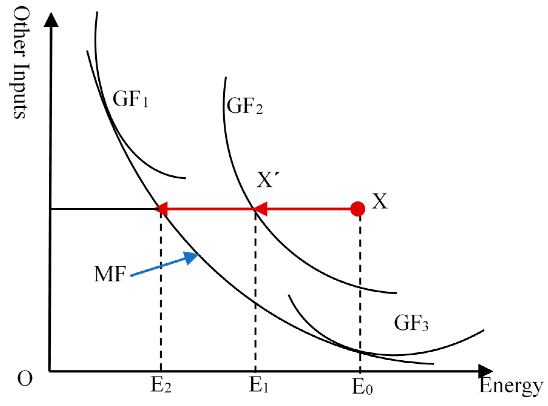
Figure 1 provides a graphical illustration of the difference between GEEI and MEEI. The curves represent the production isoquants, i.e., three for group frontiers (GF1, GF2 and GF3) and the last one for metafrontier (MF). We consider a DMU, i.e., X in Figure 1, whose energy is underutilized according to its own groupfrontier (GF2) as well as the metafrontier (MF). In this case, GEEI and MEEI of DMU X can be calculated as the ratio of and the ratio of , respectively.
Then, we show that the MTRI of DMU X can be expressed as the ratio of , reflecting the technical efficiency between groupfrontier (GF2) and the metafrontier (MF). Furthermore, if we regard as the hypothetically corresponding efficient DMU of X relative to its groupfrontier, the metatechnology ratio index of group j can be seen as a potential energy efficiency index (PEEI), which is defined as:
where
denotes the simulated Shephard energy distance function with respect to the potential DMU on one specific groupfrontier, so that PEEI can be taken as a special energy efficiency of a potential (not an actual) DMU (e.g., ). To specify this, we rewrite Equation (7) as follows:
Equation (10) reveals the links among the abovementioned three different energy efficiency indices, namely, MEEI, GEEI and PEEI, implying that the energy efficiency relative to the metafrontier can be regarded as a combination of two separate parts: GEEI for an actual DMU with respect to its own groupfrontier, and PEEI for a potential DMU on the specific groupfrontier with respective to the metafrontier. We can easily conclude that increases in MEEI may be driven by increases in GEEI or PEEI, or both of them. The implications are that, for a DMU X, it can improve its energy efficiency relative to the metafrontier through: (i) improving its energy efficiency within a specific group given that the gap between its own groupfrontier to metafrontier remains unchanged; (ii) improving its potential energy efficiency (shrinking the gap between its own groupfrontier to metafrontier) given that its group-specific energy efficiency remains unchanged; or (iii) improving the group-specific and potential energy efficiency simultaneously. It is worth noting that the terminology of PEEI is of vital importance to help further decompose the metatechnology ratio change component in a clear and convenient way.
2.2. Metafrontier Malmquist Energy Productivity Index
The Malmquist productivity index, inspired by Malmquist [51], was first theoretically approved by Caves et al. [52], and further developed by Färe et al. [53] as the product of efficiency change and technological change. Referring to Du and Lin [1], we define a Malmquist energy productivity index to explore the dynamics of total-factor energy efficiency as:
where the subscripts and denote periods and , respectively, and the superscript denotes the DMU . Following this definition and combined with Equation (10), we can express the changes of total-factor energy efficiency from periods to period in the Malmquist productivity index framework with two standard components as:
In Equation (12), MMEPI denotes the metafrontier Malmquist energy productivity index, which can be decomposed into metafrontier efficiency change index (MECI) and metafrontier technological change index (MTCI), following the benchmark decomposition framework in Färe et al. [53] or Du and Lin [1]. Accordingly, in Equation (13), GMEPI denotes the groupfrontier Malmquist energy productivity index with two components, namely, groupfrontier efficiency change index (GECI) and groupfrontier technological change index (GTCI).
We now focus on the potential Malmquist energy productivity index (PMEPI), which reflects the catch-up effect from groupfrontier to metafrontier and is in general treated as an indecomposable component (see, e.g., [27,29,30,31,32,33]). However, Chen and Yang [35,42] regarded it as a technical adjusted factor and decomposed it into i.e., pure technological catch-up (PTCU) and frontier catch-up (FCU) in an output-oriented distance function framework. According to Chen and Yang, PTCU captures the catch-up effect in technology without the ingredients of technical inefficiency from the view of a groupfrontier, and FCU implies the change in a whole band of TGR lying between the groupfrontiers and the metafrontier. Furthermore, Zhang and Wang [41] provided another terminology in the Luenberger index framework, that is, efficiency change gap (ECG) and technological change gap (TCG), which were identical to PTCU and FCU, respectively. In this paper, since PEEI is regarded as a special energy efficiency, its Malmquist productivity can thus be decomposed into two common components: efficiency change and technological change. Recalling that PEEI reflects the catch-up effect between groupfrontier and metafrontier, the above components of PMEPI are accordingly termed as efficiency catch-up index (ECUI) and technological catch-up index (TCUI). Obviously, the interpretations of the two catch-up components are much more straightforward than before from the standard decomposition framework of Malmquist productivity index.
Let us consider the relationship among MMEPI, GMEPI and PMEPI. Integrating Equations (9), and (12)–(14), we can finally obtain the MMEPI as follows:
It is easy to obtain the following equalities:
Furthermore, after reforming Equation (15), MMEPI can be expressed as:
Equation (16) reveals that the efficiency change in metafrontier Malmquist energy productivity can be seen as a product of groupfrontier efficiency change and efficiency catch-up between groupfrontier and metafrontier. Similarly, metafrontier technological change is driven by both groupfrontier technological change and potential technological catch-up. Meanwhile, Equation (17) indicates that the metafrontier Malmquist energy productivity growth is determined by the groupfrontier Malmquist energy productivity growth (relative to an actual DMU) as well as the potential Malmquist energy productivity growth (relative to a potential DMU). In this sense, an increase in MMEPI may be driven by an increase in GMEPI or PMEPI, or both of them. As such, according to Equation (15), the metafrontier Malmquist energy productivity can be regarded as a product of four specific components, namely, groupfrontier efficiency change, groupfrontier technological change, efficiency catch-up and technological catch-up.
2.3. Model Specification and Estimation
Basically, the Shephard energy distance function can be calculated by DEA or SFA. Up to date, DEA, featuring in irrespective of mandate model specification, is more widely used than SFA. However, the conventional DEA has a main drawback that it does not take statistical noises into account. In this regard, SFA seems more attractive and is increasingly employed in recent studies about energy and environmental issues, see, e.g., Zhou et al. [43], Du and Lin [1], and Filippini and Hunt [54]. When considering group heterogeneity, a so-called two-step mixed approach developed by Battese et al. [25] and O’ Donnell et al. [26] has gained increasingly popularity in the calculation of technical efficiency. As its name implies, the two-step mixed approach covers two different steps, that is, the first step is the estimation of group-specific technical efficiency by SFA, while the technical efficiency relative to the metafrontier in the second step is estimated by mathematical programming techniques rather than SFA. The methodological discrepancy weakens to some extent the advantages of SFA over DEA. Thereafter, Huang et al. [44] introduced a new two-step stochastic metafrontier approach, featuring in methodological consistency in the two estimation steps, to evaluate the production performance of world’s agriculture and Taiwanese hotel industry. We apply this approach to address energy and environmental issues in the present paper.
Referring to Du and Lin [1] and Shen and Lin [19], we use a translog function to describe the group-specific Shephard energy distance function in the first step, which is given by:
where ; and is a random variable assumed to be independent and identically distributed, that is, i.i.d . Note that there are two different implications of ; the subscript denotes periods; and the variable captures technological change over time. According to Equation (3), the Shephard energy distance function is linearly homogeneous in energy, based on which we can rewrite Equation (18) as:
where , denoting composite error; is independent of and is assumed to be following Battese and Collei [55], in which is a nonnegative random variable satisfying i.i.d . is an unknown scalar parameter, which indicates an improvement in technical efficiency if , or a decline in technical efficiency if . Additionally, represents the total periods.
Equation (19) can be estimated through employing MLE, and GEEI with respect to Equation (5) is predicted by:
Similarly, we can also estimate the metafrontier Shephard energy distance function to calculate MEEI. However, due to different data-generating processes, the above estimated metafrontier may not exactly envelope all the groupfrontiers. To address this issue, Battese et al. [25] redefined the metafrontier to be an envelope of the deterministic parts of the groupfrontiers, which was further confirmed and developed in O’ Donnell et al. [26]. However, the deterministic metafrontier function may have some limitations in terms of computation: (i) it is hard to provide a meaningful statistical interpretation to the calculated metafrontier function due to the unclear statistical properties of the estimated parameters; (ii) the mathematical programming techniques are unable to incorporate random shocks, which may result in a relatively inefficient calculation of metafrontier energy efficiency; and, more seriously, (iii) the calculation in the second step applies the estimated group frontiers rather than the theoretical ones such that the degree of bias is unknown (Huang et al. [44]; Chang et al. [56]). Consequently, Huang et al. [44] introduced a new two-step stochastic metafrontier approach, in which SFA is also utilized for the calculation of metatechnology ratio (PEEI) in the second step. In this sense, the aforementioned difficulties can be avoided. Therefore, this paper follows their methodology with a marginal extension to the input-oriented distance function framework.
Integrating Equations (8) and (9), MTRI (PEEI) can be rewritten as follows:
where denotes the actual energy input, and , denote the optimal energy input with respect to metafrontier and groupfrontier, respectively. Taking natural logarithms in both sides of Equation (21), we get:
where , that is, . Further, Equation (19) can be rewritten as:
In Equation (23), stands for the deterministic part of stochastic groupfrontier. Accordingly, can be seen as the deterministic part of stochastic metafrontier.
Recalling the relationship between the computed and true deterministic groupfrontier, we have:
Plugging Equation (24) into Equation (22), we obtain:
where , . According to Huang et al. [44], the non-negative inefficiency term can be assumed to be i.i.d . On the other hand, can be reasonably assumed to be asymptotically normally distributed with zero mean, but may not be independently, identically distributed due to the residuals, . To address this issue, the quasi-maximum likelihood estimator (QMLE) is applied instead of the standard MLE, in which the sandwich-form estimators for covariance matrix are used to obtain the correct standard errors (Huang et al. [44]; White [57]).
Consequently, PEEI can be predicted by:
With Equations (20) and (26), the estimated MEEI can be calculated according to Equation (10).
Let us switch to the calculation of energy productivity. On the one hand, groupfrontier efficiency change index and efficiency catch-up index can be calculated directly from the estimated GEEI and PEEI between periods t and t + 1.
On the other hand, the groupfrontier technological change index and technological catch-up index can be estimated following the framework introduced by Fuentes et al. [58]:
Finally, with Equations (27)–(29), MECI and MTCI can be computed according to Equation (16). Moreover, MMEPI, GMEPI and PMEPI, can be calculated following Equations (12)–(14), respectively.
3. Empirical Analysis
3.1. Data and Industrial Heterogeneity
We undertake the empirical analysis on the dynamics of China’s industrial energy efficiency at the disaggregated level over the period of 2001–2015 that covers exactly three FYPs. Since the National Standard of Industrial Classification (GB/T4754) has been amended three times during this sample period, we need to make some necessary adjustments to ensure the consistent statistical coverage of each industrial sector following the amendment framework of Chen [59]. In this regard, we finally choose 35 two-digit sub-industries listed in Table 1 for this empirical study.
The required variables include capital stock (K), labor (L) and energy (E) as inputs, and industrial gross output (Y) as the output. First, the data of capital stock and labor (numbers of employees) from 2001 to 2008 are directly acquired from Chen [59], and the other data from 2012 to 2015 are extrapolated following Chen’s methodology. The corresponding raw materials are collected from China Statistical Yearbook and China Industry Economy Statistical Yearbook. Second, energy is measured by final energy consumption, and the relevant data are collected from China Energy Statistical Yearbook. Third, the construction of industrial gross output follows Chen’s refinement framework, that is, using total gross output to solve the discrepancy in statistical coverage over different years. Furthermore, we apply IO tables (i.e., 2000, 2002, 2005, 2007, 2010, and 2012) released in Input–Output Tables of China to amend the values in both total and disaggregated gross outputs. Additionally, the nominal data on capital stock and industrial gross output have been deflated into constant price at 1990 following Chen [59].
Regarding the heterogeneity across sub-industries, this paper follows the classifications in Fan et al. [46] and Li and Lin [60], where sub-industries are divided into two groups, namely, heavy industry and light industry. The coverage of each industry is noted under Table 1: 23 sub-industries for heavy industry and 12 sub-industries for light industry.
From Table 1, the average levels of gross output (Y), capital stock (K), labor (L) and energy (E) in heavy industry are higher than those in light industry. Moreover, from the additional variables, i.e., capital intensity (K/L) and energy intensity (E/Y), we can find that heavy industry is in general more capital-intensive and energy-intensive than light industry. For example, the mean value of capital intensity in heavy industry is approximately two times higher than that in light industry. Meanwhile, the mean value of energy intensity in heavy industry is around seven times higher than that in light industry. When considering the maximum level, the energy intensity gap between heavy and light industry is even bigger, about 11 times. However, in view of the minimum level, the energy intensity in heavy industry is approximately half of that in light industry, which implies that some heavy sub-industries may be more energy efficiently used than light industry.
3.2. Estimation Results
We report the estimation results for four different frontier functions in Table 2, the former three of which are computed by MLE and the last one is estimated by QMLE. First, the “pooled” column represents that the model is estimated by pooling all the sub-industries as a whole. The “heavy” and “light” columns represent the group-specific estimates under the concept of technology heterogeneity. We use log-likelihood ratio (LR) test to analyze whether group heterogeneity is statistically significant. The LR statistic is defined by λ = −2{ln[L(H0)] − ln[L(H1)]}, where ln[L(H0)] denotes the log-likelihood value of “pooled” regression with the null hypothesis (H0) that the frontiers of different groups are identical, and ln[L(H1)] denotes the sum of log-likelihood values of both “heavy” and “light” regressions with the alternative hypothesis (H1) that the frontiers of both groups are different. The LR test listed in Table 2 rejects the null hypothesis, indicating that the frontiers of “heavy” and “light” are statistically heterogeneous. Second, apart from the listed variables in Table 1 and technology variable , we also incorporate two dummy variables, namely, dum115 and dum125, representing the 11th and the 12th FYPs, respectively. Compared with the period of 10th FYP (2001–2005), energy is more efficiently used in the periods of 2006–2010 and 2011–2015 with positive signs. Third, most of the estimated values of lnσ2 and ln[γ/(1 − γ)] for models I–IV are significant at the 1% level, confirming that technical inefficiency generally exists in the industrial sector.
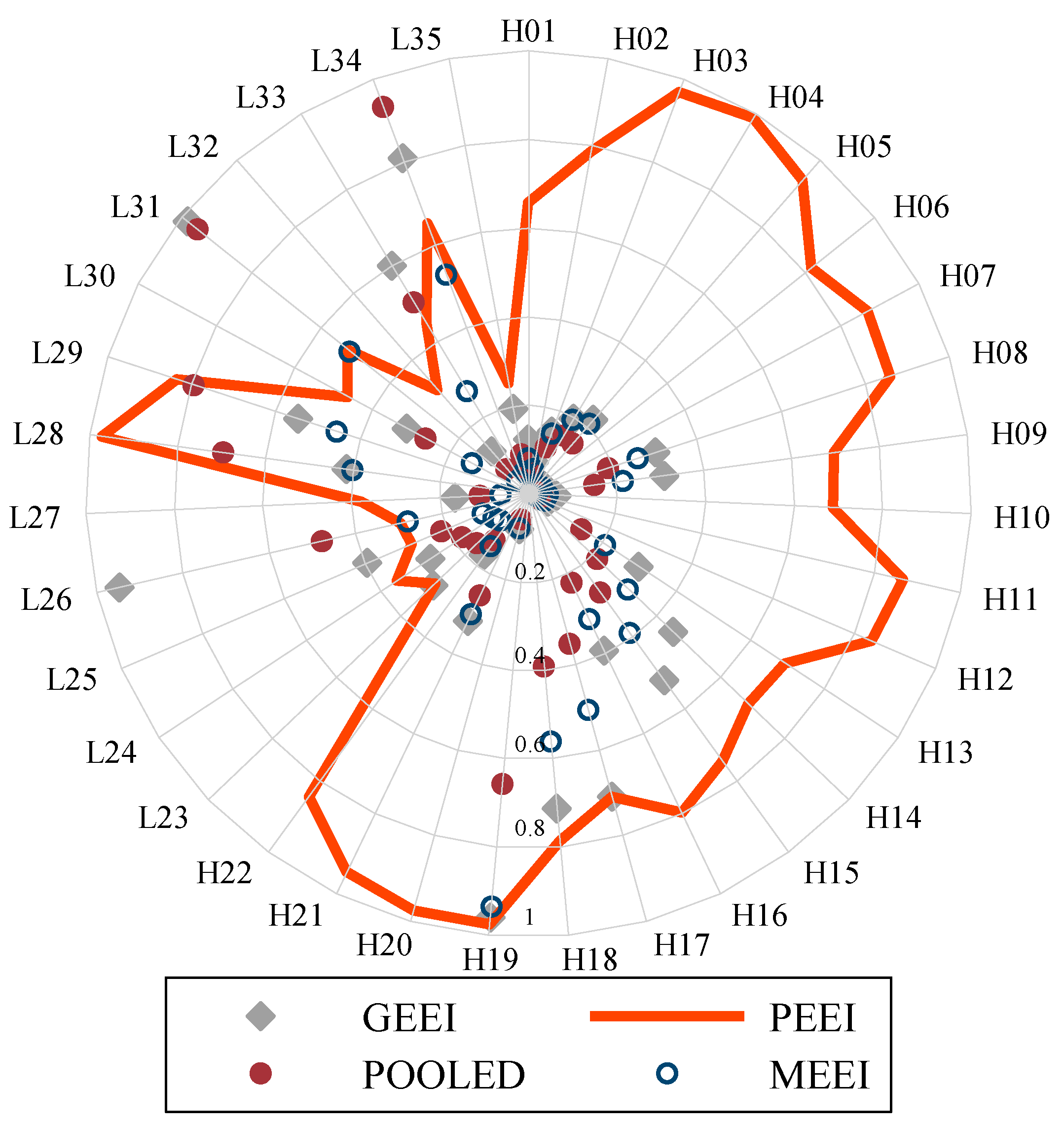
Based on the estimated parameters in Table 2, we calculate four different energy efficiency indices, that is, the pooled energy efficiency index (hereinafter POOLED), GEEI, PEEI and MEEI, and depict the average values from 2001 to 2015 in Figure 2.
It can be seen that the average values in measuring instruments manufacturing in heavy industry (H19) and furniture manufacturing in light industry (L31) are approximately equal in terms of GEEI. However, in view of MEEI, the average value in H19 stays almost unchanged while that in L31 becomes much smaller. This difference between the two typical sub-industries comes from the metatechnology. That is, the potential energy use technology in H19 is more advanced than that in L31, which leads to a bigger value of PEEI in H19 than that in L31, as shown in Figure 2. Generally, the average values of PEEI in heavy industry are higher than those in light industry, which is in line with Li and Lin [60].
In view of POOLED, light industry seems to perform better than heavy industry. For example, there are four sub-industries exceeding 0.6 in light industry (L28, L29, L31, and L34) but only one in heavy industry (H19). However, the performance of light and heavy industry becomes closer in terms of MEEI, that is, four sub-industries and three sub-industries are over 0.4, respectively. The difference between POOLED and MEEI implies that the homogeneous technology assumption is somewhat inappropriate and biased.
3.3. Decomposition Results
3.3.1. Macro-Analysis
We calculate the cumulative MMEPI and its components according to Equations (27)–(29) for the period of 2001–2005, setting 2001 as the base year. Figure 3 presents the cumulative average trends among different sub-industries in three categories, where “O”, “H” and “L” denote overall industry, heavy industry and light industry, respectively. We can see that MMEPI(O) has experienced a U-shaped change, going downward until 2006 with a minimum cumulative energy productivity of 0.825. From then on, the growth rate of MMEPI(O) becomes positive and peaks in 2015 with a maximum cumulative energy productivity of 1.250. It means that energy productivity in overall industry has increased by 25% during the past fifteen years. In general, this U-shaped development of energy productivity is in line with Du and Lin [1]. Moreover, the turning point of 2006 implies that China’s ECER program seems to take effect.
Further, Figure 3 provides more details about cumulative growth of MMEPI from three aspects. First, Figure 3a displays two MMEPIs for heavy industry and light industry in the additive manner. We find that: (i) both of them have experienced a U-shaped development, but the turning points are different, that is, 2007 and 2005, respectively; and (ii) the average cumulative values of MMEPI in light industry are generally bigger than those in heavy industry, albeit they are equal at the base year.
Second, Figure 3b plots the decomposition results based on Equation (17) in the multiplicative manner. It is noteworthy that the turning points in the cumulative growth of GMEPI and PMEPI are the same year (2007), while that in MMEPI is 2006. This difference is caused by the used averaging techniques: the average value of GMEPI multiplying that of PMEPI does not necessarily equal that of MMEPI, albeit it holds in each sub-industry. However, the comparison between GMEPI and PMEPI is meaningful. We can observe that the curve of PMEPI is above GMEPI until 2014, indicating that PMEPI performs better than GMEPI before 2014 in terms of geometric mean of cumulative energy productivity growth. However, when it turns to 2015, the cumulative growth of GMEPI slightly surpasses PMEPI. That is, on average, GMEPI performs a little better than PMEPI for the period of 2001–2015.
Third, based on Equations (12), (16) and (27)–(29), Figure 3c presents the decomposition results of MECI and MTCI also in the multiplicative manner. We can see that MECI undergoes a decline during the sample period, which is different from the U-shaped change of MTCI as well as the other components in Figure 3a,b. This means that energy efficiency has generally deteriorated over time, whereas after 2004 energy technological progress is so significant that it finally drives up the energy productivity from 2006 on.
According to Equations (15) and (27)–(29), we further provide four specific components and their contributions for the cumulative metafrontier Malmquist energy productivity growth in Table 3. In the column of “Cumulative growth index”, MMEPI is decomposed into four components, namely, GECI, GTCI ECUI and TCUI. For the averaging reasons as discussed above, MMEPI is not necessarily equal to the product of these four components. Accordingly, we take natural logarithm of productivity growth in order to analyze the relative contributions of different components.
First, in the 10th FYP period (2001–2005), MMEPI has experienced a general decline in heavy industry, light industry and also overall industry. Specially, only GECI in light industry witnesses a positive growth in this period. Second, during the 11th FYP period (2006–2010), the metafrontier Malmquist energy productivity in light industry shows a productivity gain, while that in heavy industry and overall industry suffers a productivity loss. However, we observe that average values of MMEPI in heavy industry and overall industry for 11th FYP period are bigger than those for 10th FYP period, implying that energy productivity starts to improve. Third, even bigger improvements are made in the 12th FYP period in all groups, and the total contributions of technological change components (GTCI and TCUI, the same below) are bigger than those of efficiency change components (GECI and ECUI, the same below).
Finally, during the period of 2001–2015, all categories have experienced an improvement in the metafrontier Malmquist energy productivity, whereas the components perform somewhat differently. For example, in heavy industry, technological change components and efficiency change components make positive and negative contributions to energy productivity growth respectively, and the former overtakes the latter, resulting in an improvement in energy productivity. Among these four components, GECI is the biggest (negative) contributor. Similarly, in overall industry, the positive contributions of technological change components surpass the negative contributions of efficiency change components, but GTCI becomes the biggest (positive) contributor. However, the picture for the light industry is quite different. That is, the contribution of GECI is positive while that of TUCI is negative, albeit the total contributions of technological change components are bigger than those of efficiency change components. Parallel to overall industry, GTCI is also the biggest (positive) contributor in light industry.
Furthermore, Figure 4 describes the dynamic contributions of four components for the cumulative metafrontier Malmquist energy productivity growth with 2001 as the base year. We can see that the cumulative efficiency change components (GECI and ECUI) contribute negatively to energy productivity growth over time, while the contributions of cumulative technological change components (GTCI and TCUI) turn from negative to positive during the sample period. Specifically, TCUI remains the biggest (negative) contributor to energy productivity growth until 2006. After, GECI takes the lead in energy productivity growth for the period of 2007–2010. GTCI begins to dominate the energy productivity growth and maintains ahead in the 12th FYP period.
Comparatively, for the period of 2001–2015, GTCI makes the biggest contribution to energy productivity growth, followed by TCUI, then ECUI and GECI, which are approximately equal. Moreover, the former two technological change components contribute positively to energy productivity growth, whereas the latter two efficiency change components make the negative contributions. It means that: (i) overall industry has experienced a significant technological progress and suffered a long-run deterioration in energy efficiency, indicating that sub-industries tend to adopt new technologies rather than make full use of the existing technologies; (ii) group-specific technology has advanced faster than metatechnology, implying that low-tech sub-industries seem to be more willing to approach new technologies than high-tech sub-industries; and (iii) the managerial inefficiency almost equally exists in the utilization of energy technologies for both low-tech and high-tech sub-industries.
3.3.2. Sectoral-Analysis
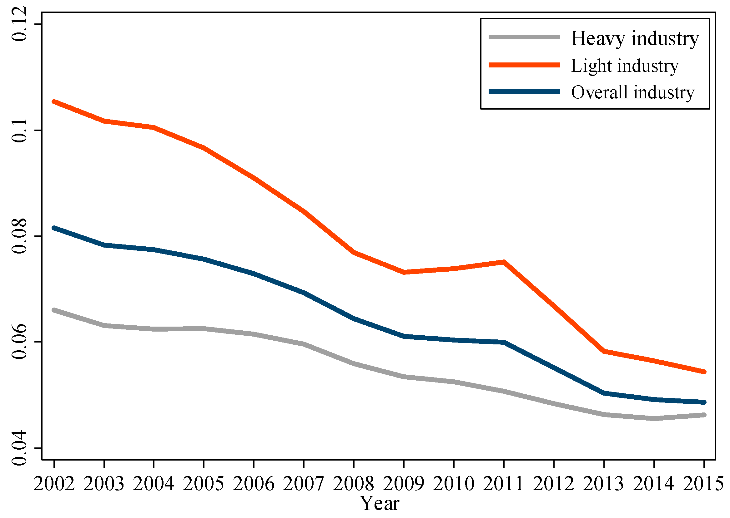
Table 4 reports the calculation results of MMEPI for all sub-industries in the period of 2001–2015. In general, the average values of MMEPI in different groups have increased over time, indicating that energy productivity has been improved for the past fifteen years. According to the geometric mean of MMEPI from 2001 to 2015, light industry has performed better than heavy industry, both of which grow at around 0.93% and 1.64% annually. This result is coincident with what it shows in Figure 3a.
We also find that 19 out of 35 sub-industries have suffered an energy productivity loss in terms of geometric mean of MMEPI from 2001 to 2015. Among these productivity loss sub-industries, heavy industry and light industry account for 13 and 6 sub-industries, respectively. In contrast, the remaining 16 of 35 sub-industries, covering nine heavy industries and seven light industries, have experienced an increase in energy productivity. These results indicate that, heavy industry is more vulnerable to suffer productivity loss than light industry, while both of them are approximately equal in achieving energy productivity gain.
As for individual sub-industries, Electricity production (H20) and Gas production (H21) have the best productivity growth performance in terms of geometric mean of MMEPI, with values of 1.117 and 1.096 respectively. On the contrary, Culture, education and sport activities manufacturing (L34), Leather manufacturing (L29), and Furniture manufacturing (L31) have suffered the biggest energy productivity loss, with geometric mean values of 0.865, 0.897 and 0.901 respectively. These ranks are similar to those of green productivity growth calculated under the Malmquist index framework in Li and Lin [47], albeit most of the sub-industries had positive productivity growth from 1998 to 2011.
In brief, there seems to be a paradox. That is, the average energy productivity growth of heavy industry is lower than that of light industry, however, the two best productivity performance sub-industries belong to heavy industry and the three worst productivity performance sub-industries belong to light industry. On the one hand, it has some clues from the minimum level of energy intensity for heavy industry and light industry in Table 1, implying that the most energy efficiently used sub-industry may come from heavy industry rather than light industry. On the other hand, to further understand this issue, we next explore the driving forces on energy productivity growth in Figure 5 and Figure 6.
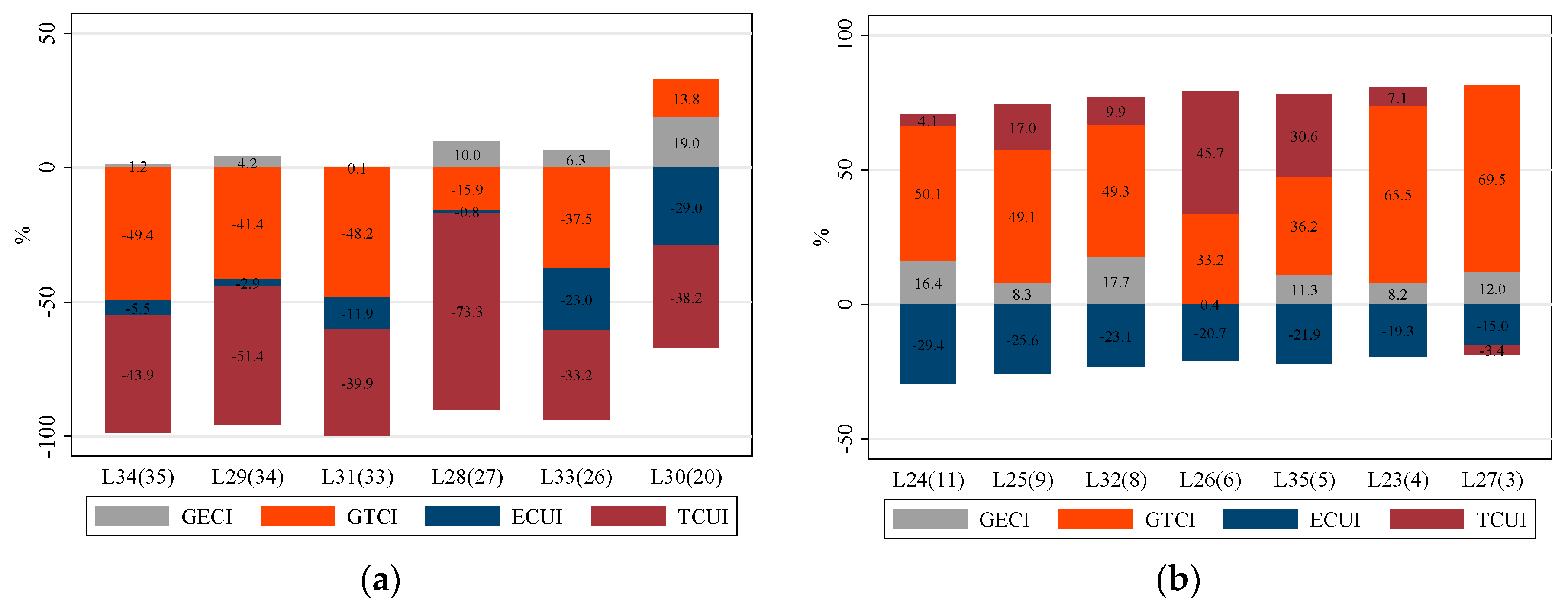
The contributions of different drivers for metafrontier Malmquist energy productivity growth are shown in Figure 5 and Figure 6, classified by: (a) productivity loss; and (b) productivity gain. It is worth noting that the contributions are calculated the same way as in Table 3 by taking natural logarithms of the cumulative growth of different components. The numbers in brackets denote the ranks of cumulative productivity growth from 2001 to 2015.
We can see that, in Figure 5 for heavy industry, efficiency change components (GECI and ECUI) contribute negatively to energy productivity growth, implying that the existing technologies are not efficiently used in heavy industry. That is, energy managerial efficiency needs to improve urgently.
Specifically, in Figure 5a, of 13 sub-industries, GECI makes the biggest contributions to energy productivity growth in eight sub-industries; GTCI takes the lead in four sub-industries; TCUI dominates energy productivity growth only in Measuring instruments manufacturing (H19). Moreover, we can find that GMEPI (GECI and GTCI) controls the energy productivity loss in these sub-industries. On the other hand, in Figure 5b, technological change components become the dominating factor of energy productivity growth with positive contributions except for Communication equipment manufacturing (H18), in which GTCI makes a negative contribution to the growth of energy productivity (−3.4%).
As for the two best productivity performance sub-industries, namely, Electricity production (H20) and Gas production (H21), we can see that technological change components play an overwhelming role in energy productivity growth, accounting for 75.8% and 82.5%, respectively. Furthermore, the productivity growth is mainly driven by the inter-group technological progress in H20 (TCUI, 42.5%) while by intra-group technological progress in H21 (GTCI, 53.8%). Meanwhile, we can also observe that the contribution of ECUI to the growth of energy productivity is negligible.
We plot in Figure 6 the different contributions of four components for MMEPI in light industry. Compared with Figure 5, GECI turns to play a positive role in energy productivity growth in light industry, albeit ECUI still contributes negatively to energy productivity growth in all light sub-industries.
In Figure 6a, technological change components (GTCI and TCUI) contribute most to the energy productivity loss in all sub-industries. Specially, in the three worst productivity performance sub-industries, namely, Culture, education and sport activities manufacturing (L34), Leather manufacturing (L29) and Furniture manufacturing (L31), the total contributions of technological change components are −93.3%, −92.8% and −88.8%, respectively. Recalling those two best productivity performance sub-industries (H20 and H21) in Figure 5b, we can conclude that in those sub-industries technological progress or regress determines energy productivity gain or loss.
In Figure 6b, apart from GECI, GTCI and TCUI also contribute positively to energy productivity growth in light industry except for Textile industry (L27) with a negative contribution of TCUI (−3.4%). Moreover, technological change components are the biggest contributor for productivity growth, as in Figure 5b and Figure 6a. In addition, GTCI dominates the increase of MMEPI in all light sub-industries except for Tobacco manufacturing (L26), in which TCUI is the biggest contributor accounting for 45.7%. It means that the energy productivity gains in light industry are mainly due to the intra-group technological progress.
To sum up, we provide the numbers of dominant contributor of the metafrontier Malmquist energy productivity growth in the 35 sub-industries in Table 5. First, 20 out of 35 sub-industries are dominated by GMEPI for energy productivity growth, and PMEPI controls the remaining 15 sub-industries. Moreover, GMEPI mainly leads to a productivity loss in heavy industry but a productivity gain in light industry; in contrast, PMEPI mainly makes positive contributions to energy productivity gain in heavy industry but negative contributions to energy productivity loss in light industry. Second, energy productivity growth in the vast majority of sub-industries is dominantly driven by MTCI; the remaining seven sub-industries are governed by MECI for productivity loss only, implying that the productivity loss may be caused by the bad management of the utilization of existing technologies. Third, as for individual contributors, GTCI performs better than others with 15 sub-industries, followed by GECI (11), and then TCUI (9). It is worth noting that: (i) no sub-industry is dominated by ECUI for productivity growth; and (ii) GECI makes most and negative contributions to productivity growth in three heavy sub-industries, albeit they experience a productivity gain.
Finally, we depict the dynamic trends of coefficients of variation (CVs) for cumulative MMEPI in different groups in Figure 7. We can observe that the CVs in overall industry show a falling trend, indicating that metafrontier Malmquist energy productivity growth in all sub-industries tends to converge over time, which is known as σ-convergence. Moreover, we can also find that the CVs of energy productivity growth in heavy industry and light industry are generally decreasing over time, and light industry seems to converge faster than heavy industry during the sample period.
4. Conclusions
In this paper, metafrontier energy efficiency consists of groupfrontier energy efficiency and potential energy efficiency, the latter of which is previously termed as technology gap ratio. Accordingly, metafrontier Malmquist energy productivity is decomposed into groupfrontier Malmquist energy productivity (i.e., groupfrontier efficiency change and groupfrontier technological change) and potential Malmquist energy productivity (i.e., efficiency catch-up and technological catch-up). Furthermore, a newly developed two-step stochastic metafrontier analysis technique is applied for the calculation of energy efficiency and productivity. The developed approach is used to compare the energy productivity growth of 35 sub-industries in China’s industrial sector for the period of 2001–2015. The main empirical results are shown as follows.
- (1)
- In view of metafrontier Malmquist energy productivity, overall industry has witnessed a 25% cumulative growth and a U-shaped trend bottoming out in 2006, which may indicate that the ECER programs are effective in the periods of 11th and 12th FYPs. Meanwhile, 19 sub-industries have suffered an energy productivity loss, and the remaining 16 sub-industries have experienced an energy productivity gain.
- (2)
- From the technology heterogeneity perspective, light industry outperforms heavy industry in metafrontier Malmquist energy productivity growth, while groupfrontier Malmquist energy productivity growth is on average a little higher than potential Malmquist energy productivity growth, indicating that the intra-group and inter-group energy productivity develops roughly in balance as a whole.
- (3)
- As for individual components, groupfrontier technological change makes the biggest contribution to energy productivity growth (43.4%), followed by technological catch-up (21.8%), efficiency catch-up (−17.4%) and groupfrontier efficiency change (−17.1%). That is, it is technological change that dominates the energy productivity growth, implying that the existing technologies are not utilized sufficiently and the management efficiency needs to improve. Furthermore, groupfrontier technological change makes positive (mainly negative) contributions in productivity gain (loss) sub-industries; technological catch-up works like groupfrontier technological change, both of which dominate the growth of energy productivity in 28 out of 35 sub-industries; efficiency catch-up contributes negatively to all the sub-industries; groupfrontier efficiency change plays a negative (positive) role in energy productivity growth for heavy (light) industry.
- (4)
- There exists σ-convergence of metafrontier Malmquist energy productivity growth in heavy industry and light industry as well as overall industry, implying that the energy efficiency laggards can catch up the energy efficiency leaders in the future, which is line with the concept of metafrontier.
These results indicate that, to perfectly fulfill the ECER targets, the Chinese government should pay more attention to heterogeneous energy policies for heavy industry and light industry. Moreover, general technologies for the improvement of energy efficiency in both heavy and light industries need to be better adopted and diffused. In particular, the management of the existing metatechnology needs urgent improvement since the efficiency catch-up component contributes negatively to all sub-industries.
There are three possible directions for future research. First, to capture environmental effect, pollutants could be incorporated into the present framework to explore environmentally sensitive energy efficiency and productivity. Second, the global Malmquist productivity index may be integrated into the present decomposition framework, so that more insights might be explored into the energy productivity growth. Third, this paper mainly investigates group heterogeneity with a two-step stochastic metafrontier analysis approach. Moreover, individual heterogeneity might also be captured and addressed by, e.g., the “true fixed effects” model suggested by Greene [61] or the within-MLE approach introduced by Chen et al. [36]. That is, a new parametric approach may be developed to solve the problems of individual heterogeneity as well as group heterogeneity.
Acknowledgments
This paper is supported by the National Natural Science Foundation of China (Nos. 71273074 and 71673067).
Author Contributions
Lizhan Cao designed the research and wrote this manuscript. Zhongying Qi and Junxia Ren participated in discussion and provided some valuable suggestions. All authors read and approved the final manuscript.
Conflicts of Interest
The authors declare no conflict of interest.
References
- Petroleum, B. Statistical Review of World Energy. Available online: http://www.bp.com/content/dam/bp/en/corporate/pdf/energy-economics/statistical-review-2017/bp-statistical-review-of-world-energy-2017-full-report.pdf (accessed on 19 June 2017).
- National Bureau of Statistics of China. Available online: http://data.stats.gov.cn/easyquery.htm?cn=C01 (accessed on 15 May 2017).
- National Development and Reform Commission. Available online: http://www.sdpc.gov.cn/zcfb/zcfbtz/201701/t20170117_835278.html (accessed on 15 May 2017).
- Hu, J.L.; Wang, S.C. Total-factor energy efficiency of regions in China. Energy Policy 2006, 17, 3206–3217. [Google Scholar] [CrossRef]
- Zhou, P.; Ang, B.W. Linear programming models for measuring economy-wide energy efficiency performance. Energy Policy 2008, 8, 2911–2916. [Google Scholar] [CrossRef]
- Li, L.B.; Hu, J.L. Ecological total-factor energy efficiency of regions in China. Energy Policy 2012, 46, 216–224. [Google Scholar] [CrossRef]
- Zhou, P.; Wu, F.; Zhou, D.Q. Total-factor energy efficiency with congestion. Annu. Oper. Res. 2015, 255, 1–16. [Google Scholar] [CrossRef]
- Zhou, D.Q.; Wu, F.; Zhou, X.; Zhou, P. Output-specific energy efficiency assessment: A data envelopment analysis approach. Appl. Energy 2016, 177, 117–126. [Google Scholar] [CrossRef]
- Zhao, L.; Zha, Y.; Liang, N.; Liang, L. Data envelopment analysis for unified efficiency evaluation: An assessment of regional industries in China. J. Clean. Prod. 2016, 113, 695–704. [Google Scholar] [CrossRef]
- Oliveira, R.; Camanho, A.S.; Zanella, A. Expanded eco-efficiency assessment of large mining firms. J. Clean. Prod. 2017, 142, 2364–2373. [Google Scholar] [CrossRef]
- Wu, F.; Fan, L.W.; Zhou, P.; Zhou, D.Q. Industrial energy efficiency with CO2 emissions in China: A nonparametric analysis. Energy Policy 2012, 49, 164–172. [Google Scholar] [CrossRef]
- Du, K.; Lin, B. International comparison of total-factor energy productivity growth: A parametric Malmquist index approach. Energy 2017, 118, 481–488. [Google Scholar] [CrossRef]
- Chang, T.P.; Hu, J.L. Total-factor energy productivity growth, technical progress, and efficiency change: An empirical study of China. Appl. Energy 2010, 10, 3262–3270. [Google Scholar] [CrossRef]
- Wang, H.; Zhou, P.; Zhou, D.Q. Scenario-based energy efficiency and productivity in China: A non-radial directional distance function analysis. Energy Econ. 2013, 40, 795–803. [Google Scholar] [CrossRef]
- Zhou, D.Q.; Wang, Q.; Su, B.; Zhou, P.; Yao, L.X. Industrial energy conservation and emission reduction performance in China: A city-level nonparametric analysis. Appl. Energy 2016, 166, 201–209. [Google Scholar] [CrossRef]
- Li, K.; Lin, B. Impact of energy conservation policies on the green productivity in China’s manufacturing sector: Evidence from a three-stage DEA model. Appl. Energy 2016, 168, 351–363. [Google Scholar] [CrossRef]
- Wang, H.; Ang, B.W.; Wang, Q.W.; Zhou, P. Measuring energy performance with sectoral heterogeneity: A non-parametric frontier approach. Energy Econ. 2017, 62, 70–78. [Google Scholar] [CrossRef]
- Wang, K.; Wei, Y.M. Sources of energy productivity change in China during 1997–2012: A decomposition analysis based on the Luenberger productivity indicator. Energy Econ. 2016, 54, 50–59. [Google Scholar] [CrossRef]
- Shen, X.; Lin, B. Total Factor Energy Efficiency of China’s Industrial Sector: A Stochastic Frontier Analysis. Sustainability 2017, 4, 646. [Google Scholar] [CrossRef]
- Balk, B.M. Scale efficiency and productivity change. J. Prod. Anal. 2001, 3, 159–183. [Google Scholar] [CrossRef]
- Pantzios, C.J.; Karagiannis, G.; Tzouvelekas, V. Parametric decomposition of the input-oriented Malmquist productivity index: With an application to Greek aquaculture. J. Prod. Anal. 2011, 1, 21–31. [Google Scholar] [CrossRef]
- Hayami, Y. Sources of Agricultural Productivity Gap among Selected Countries. Am. J. Agric. Econ. 1969, 3, 564–575. [Google Scholar] [CrossRef]
- Hayami, Y.; Ruttan, V.W. Agricultural productivity differences among countries. Am. Econ. Rev. 1970, 5, 895–911. [Google Scholar]
- Battese, G.E.; Rao, D.S.P. Technology Gap, Efficiency, and a Stochastic Metafrontier Function. Int. J. Bus. Econ. 2002, 2, 87–93. [Google Scholar]
- Battese, G.E.; Rao, D.S.P.; O’Donnell, C.J. A Metafrontier Production Function for Estimation of Technical Efficiencies and Technology Gaps for Firms Operating Under Different Technologies. J. Prod. Anal. 2004, 1, 91–103. [Google Scholar] [CrossRef]
- O’Donnell, C.J.; Rao, D.S.P.; Battese, G.E. Metafrontier frameworks for the study of firm-level efficiencies and technology ratios. Empir. Econ. 2008, 2, 231–255. [Google Scholar] [CrossRef]
- Oh, D.H. A metafrontier approach for measuring an environmentally sensitive productivity growth index. Energy Econ. 2010, 1, 146–157. [Google Scholar] [CrossRef]
- Pastor, J.T.; Lovell, C.A.K. A global Malmquist productivity index. Econ. Lett. 2005, 2, 266–271. [Google Scholar] [CrossRef]
- Chung, Y.; Heshmati, A. Measurement of environmentally sensitive productivity growth in Korean industries. J. Clean. Prod. 2014, 104, 380–391. [Google Scholar] [CrossRef]
- Munisamy, S.; Arabi, B. Eco-efficiency change in power plants: Using a slacks-based measure for the meta-frontier Malmquist–Luenberger productivity index. J. Clean. Prod. 2015, 105, 218–232. [Google Scholar] [CrossRef]
- Wang, H.; Zhou, P.; Wang, Q. Constructing slacks-based composite indicator of sustainable energy development for China: A meta-frontier nonparametric approach. Energy 2016, 101, 218–228. [Google Scholar] [CrossRef]
- Li, K.; Song, M. Green Development Performance in China: A Metafrontier Non-Radial Approach. Sustainability 2016, 3, 219. [Google Scholar] [CrossRef]
- Fei, R.; Lin, B. Energy efficiency and production technology heterogeneity in China’s agricultural sector: A meta-frontier approach. Technol. Forecast. Soc. Chang. 2016, 109, 25–34. [Google Scholar] [CrossRef]
- Li, K.; Lin, B. Metafroniter energy efficiency with CO2 emissions and its convergence analysis for China. Energy Econ. 2015, 48, 230–241. [Google Scholar] [CrossRef]
- Chen, K.H.; Yang, H.Y. Extensions of the metafrontier Malmquist productivity index: An empirical study with cross-country macro-data. Taiwan Econ. Rev. 2008, 4, 551–588. [Google Scholar]
- Chen, Y.Y.; Schmidt, P.; Wang, H.J. Consistent estimation of the fixed effects stochastic frontier model. J. Econom. 2014, 2, 65–76. [Google Scholar] [CrossRef]
- Zhang, Z.; Ye, J. Decomposition of environmental total factor productivity growth using hyperbolic distance functions: A panel data analysis for China. Energy Econ. 2015, 47, 87–97. [Google Scholar] [CrossRef]
- Cuesta, R.A.; Lovell, C.A.K.; Zofío, J.L. Environmental efficiency measurement with translog distance functions: A parametric approach. Ecol. Econ. 2009, 8, 2232–2242. [Google Scholar] [CrossRef]
- Lin, E.Y.Y.; Chen, P.Y.; Chen, C.C. Measuring green productivity of country: A generlized metafrontier Malmquist productivity index approach. Energy 2013, 55, 340–353. [Google Scholar]
- Orea, L. Parametric decomposition of a generalized Malmquist productivity index. J. Prod. Anal. 2002, 1, 5–22. [Google Scholar] [CrossRef]
- Zhang, N.; Wang, B. A deterministic parametric metafrontier Luenberger indicator for measuring environmentally-sensitive productivity growth: A Korean fossil-fuel power case. Energy Econ. 2015, 51, 88–98. [Google Scholar] [CrossRef]
- Chen, K.H.; Yang, H.Y. A cross-country comparison of productivity growth using the generalised metafrontier Malmquist productivity index: With application to banking industries in Taiwan and China. J. Prod. Anal. 2011, 3, 197–212. [Google Scholar] [CrossRef]
- Zhou, P.; Ang, B.W.; Zhou, D.Q. Measuring economy-wide energy efficiency performance: A parametric frontier approach. Appl. Energy 2012, 1, 196–200. [Google Scholar] [CrossRef]
- Huang, C.J.; Huang, T.H.; Liu, N.H. A new approach to estimating the metafrontier production function based on a stochastic frontier framework. J. Prod. Anal. 2014, 3, 241–254. [Google Scholar] [CrossRef]
- Chen, S.; Golley, J. ‘Green’ productivity growth in China’s industrial economy. Energy Econ. 2014, 44, 89–98. [Google Scholar] [CrossRef]
- Fan, M.; Shao, S.; Yang, L. Combining global Malmquist-Luenberger index and generalized method of moments to investigate industrial total factor CO2 emission performance: A case of Shanghai (China). Energy Policy 2015, 79, 189–201. [Google Scholar] [CrossRef]
- Li, K.; Lin, B. Measuring green productivity growth of Chinese industrial sectors during 1998–2011. China Econ. Rev. 2015, 36, 279–295. [Google Scholar] [CrossRef]
- Emrouznejad, A.; Yang, G. A framework for measuring global Malmquist–Luenberger productivity index with CO2 emissions on Chinese manufacturing industries. Energy 2016, 115, 840–856. [Google Scholar] [CrossRef]
- Yang, M.; Yang, F. Energy-Efficiency Policies and Energy Productivity Improvements: Evidence from China’s Manufacturing Industry. Emerg. Mark. Financ. Trade 2016, 6, 1395–1404. [Google Scholar] [CrossRef]
- Lin, B.; Du, K. Technology gap and China’s regional energy efficiency: A parametric metafrontier approach. Energy Econ. 2013, 40, 529–536. [Google Scholar] [CrossRef]
- Malmquist, S. Index numbers and indifference surfaces. Traba. Estad. 1953, 2, 209–242. [Google Scholar] [CrossRef]
- Caves, D.W.; Christensen, L.R.; Diewert, W.E. Multilateral comparisons of output, input, and productivity using superlative index numbers. Econ. J. 1982, 365, 73–86. [Google Scholar] [CrossRef]
- Fare, R.; Grosskopf, S.; Norris, M.E. Productivity Growth, Technical Progress, and Efficiency Change in Industrialized Countries. Am. Econ. Rev. 1994, 1, 66–83. [Google Scholar]
- Filippini, M.; Hunt, L.C. Measurement of energy efficiency based on economic foundations. Energy Econ. 2015, 52, S5–S16. [Google Scholar] [CrossRef]
- Battese, G.E.; Coelli, T.J. Frontier production functions, technical efficiency and panel data: With application to paddy farmers in India. J. Prod. Anal. 1992, 3, 153–169. [Google Scholar] [CrossRef]
- Chang, B.G.; Huang, T.H.; Kuo, C.Y. A comparison of the technical efficiency of accounting firms among the US, China, and Taiwan under the framework of a stochastic metafrontier production function. J. Prod. Anal. 2015, 3, 337–349. [Google Scholar] [CrossRef]
- White, H. Maximum likelihood estimation of misspecified models. Econom. J. Econom. Soc. 1982, 50, 1–25. [Google Scholar] [CrossRef]
- Fuentes, H.J.; Grifell-Tatjé, E.; Perelman, S. A Parametric Distance Function Approach for Malmquist Productivity Index Estimation. J. Prod. Anal. 2001, 2, 79–94. [Google Scholar] [CrossRef]
- Chen, S. Reconstruction of sub-industrial statistical data in China (1980–2008). China Econ. Quart. 2011, 3, 735–776. [Google Scholar]
- Li, J.; Lin, B. Ecological total-factor energy efficiency of China’s heavy and light industries: Which performs better? Renew. Sustain. Energy Rev. 2017, 72, 83–94. [Google Scholar] [CrossRef]
- Greene, W. Fixed and random effects in stochastic frontier models. J. Prod. Anal. 2005, 1, 7–32. [Google Scholar] [CrossRef]
Figure 1.
Technology frontiers and different forms of energy efficiency.

Figure 2.
The average energy efficiency with different indices.

Figure 3.
Cumulative metafrontier Malmquist energy productivity growth and its components: (a) heavy and light industries; (b) groupfrontier and potential productivity indices; and (c) efficiency and technology components.
Figure 3.
Cumulative metafrontier Malmquist energy productivity growth and its components: (a) heavy and light industries; (b) groupfrontier and potential productivity indices; and (c) efficiency and technology components.
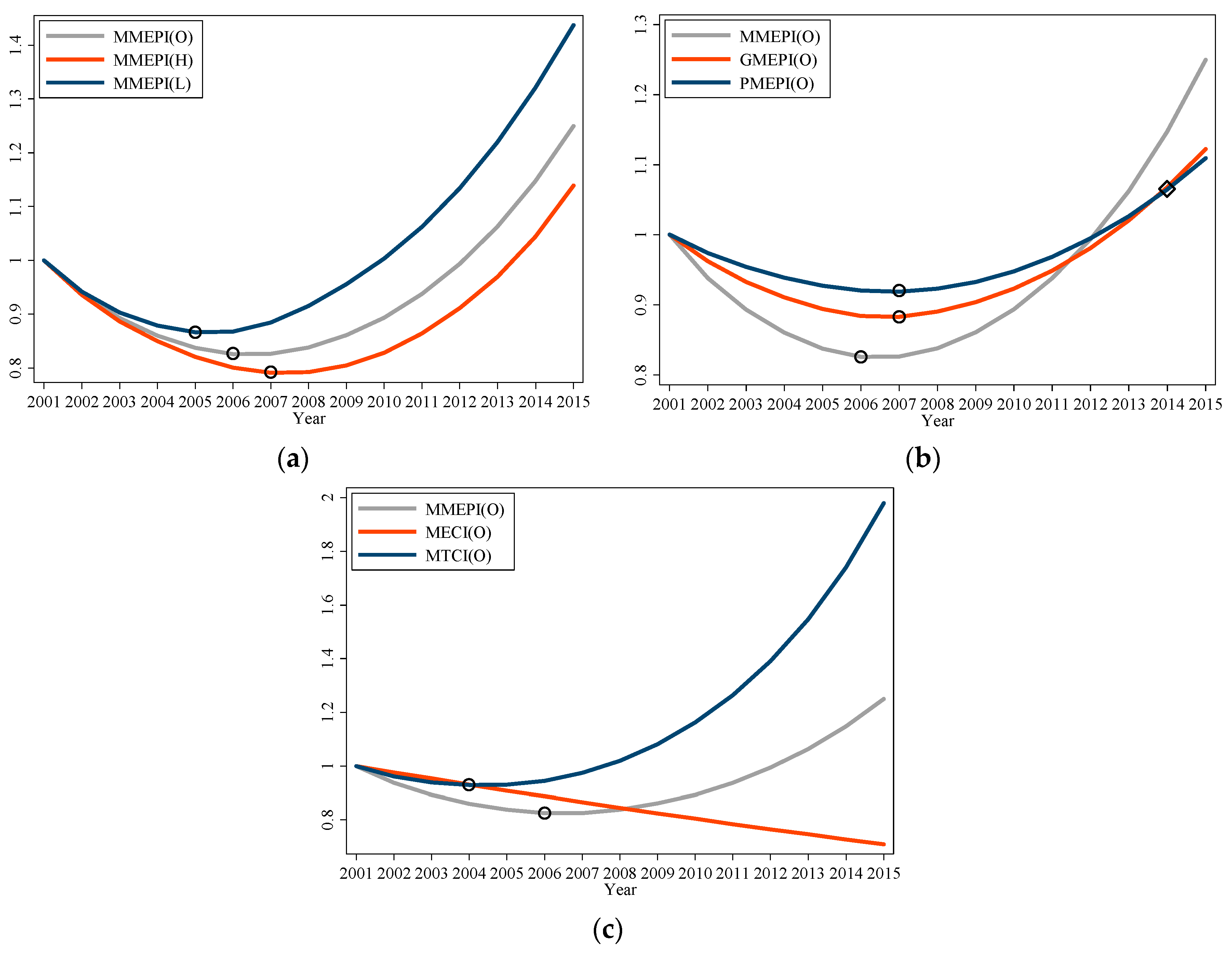
Figure 4.
Dynamic contributions of different components for cumulative MMEPI in overall industry.
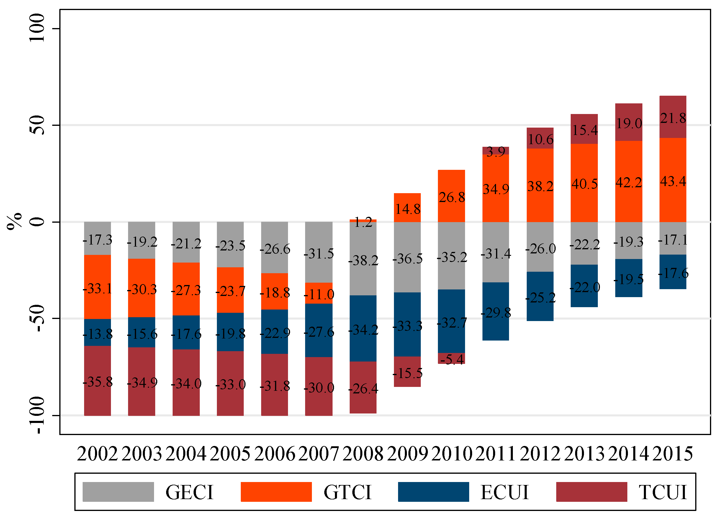
Figure 5.
Contributions of different components for MMEPI in heavy industry: (a) productivity loss; and (b) productivity gain.
Figure 5.
Contributions of different components for MMEPI in heavy industry: (a) productivity loss; and (b) productivity gain.
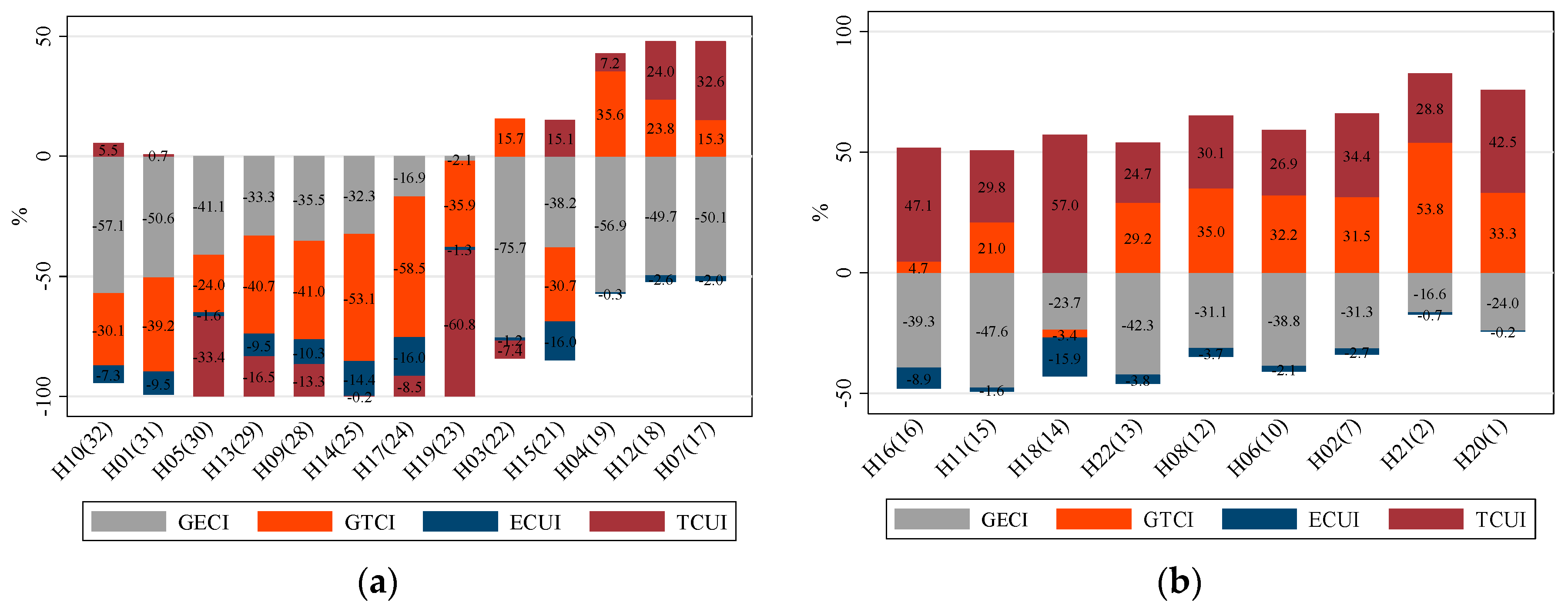
Figure 6.
Contributions of different components for MMEPI in light industry: (a) productivity loss; and (b) productivity gain.
Figure 6.
Contributions of different components for MMEPI in light industry: (a) productivity loss; and (b) productivity gain.

Figure 7.
Dynamic change of coefficients of variation for cumulative MMEPI in different groups.


Table 1.
Summary statistics and industry classification.
| Variables | Units | Heavy industry | Light industry | ||||||||
|---|---|---|---|---|---|---|---|---|---|---|---|
| Obs. | Mean | Std. dev. | Min | Max | Obs. | Mean | Std. dev. | Min | Max | ||
| Y | 109 RMB | 330 | 1.254 | 2.078 | 0.009 | 15.413 | 195 | 0.541 | 0.456 | 0.056 | 2.433 |
| K | 109 RMB | 330 | 0.372 | 0.476 | 0.016 | 3.628 | 195 | 0.118 | 0.109 | 0.005 | 0.599 |
| L | 109 Persons | 330 | 0.036 | 0.028 | 0.002 | 0.108 | 195 | 0.027 | 0.022 | 0.002 | 0.095 |
| E | 109 TCE | 330 | 0.769 | 1.296 | 0.015 | 8.034 | 195 | 0.143 | 0.162 | 0.009 | 0.730 |
| K/L | RMB/Person | 330 | 15.019 | 18.309 | 1.130 | 110.882 | 195 | 6.698 | 6.887 | 0.373 | 30.250 |
| E/Y | TCE/RMB | 330 | 1.885 | 2.624 | 0.020 | 13.608 | 195 | 0.266 | 0.227 | 0.038 | 1.229 |
Note: (1) Heavy industry covers: Coal mining and washing (H01), Oil and natural gas extracting (H02), Ferrous metal mining (H03), Non-ferrous metal mining (H04), Non-metal mining (H05), Oil processing, coking and nuclear fuel processing (H06), Chemical materials and products manufacturing (H07), Medicines manufacturing (H08), Rubber and plastics manufacturing (H09), Non-metallic Mineral Products manufacturing (H10), Ferrous metal smelting and pressing (H11), Non-ferrous metal smelting and pressing (H12), Metal products manufacturing (H13), General purpose manufacturing (H14), Special purpose manufacturing (H15), Transport equipment manufacturing (H16), Electrical machinery and equipment manufacturing (H17), Communication equipment manufacturing (H18), Measuring instruments manufacturing (H19), Electricity production (H20), Gas production (H21), and Water production (H22). (2) Light industry covers: Food processing (L23), Food manufacturing (L24), Beverages manufacturing (L25), Tobacco manufacturing (L26), Textile industry (L27), Textile clothes, shoes and caps (L28), Leather manufacturing (L29), Timber and wood processing (L30), Furniture manufacturing (L31), Paper industry (L32), Printing and intermediary replication (L33), Culture, education and sport activities manufacturing (L34), and Chemical fibers manufacturing (L35).
Table 2.
Estimations of pooled frontier, groupfrontiers and metafrontier functions.
| First Step | Second Step | |||||||
|---|---|---|---|---|---|---|---|---|
| I Pooled a | II Heavy a | III Light a | IV Metafrontier b | |||||
| lnk | 0.221 ** | 0.110 | 0.868 *** | 0.138 | −0.669 ** | 0.308 | 0.124 | 0.142 |
| lnl | −0.720 *** | 0.235 | −1.673 *** | 0.238 | 0.832 ** | 0.377 | −0.969 ** | 0.392 |
| lny | −0.531 *** | 0.136 | −0.221 * | 0.137 | −1.337 *** | 0.361 | −0.399 ** | 0.181 |
| t | −0.057 *** | 0.021 | −0.168 *** | 0.026 | 0.114 *** | 0.042 | −0.056 ** | 0.023 |
| (lnk)2 | −0.071 *** | 0.015 | −0.058 ** | 0.025 | −0.124 *** | 0.050 | −0.075 *** | 0.009 |
| (lnl)2 | −0.140 *** | 0.039 | −0.311 *** | 0.042 | −0.026 | 0.045 | −0.171 *** | 0.055 |
| (lny)2 | 0.024 | 0.022 | 0.017 | 0.020 | −0.145 | 0.134 | 0.021 | 0.018 |
| t2 | 0.001 | 0.001 | 0.001** | 0.001 | −0.003** | 0.001 | 0.000 | 0.000 |
| lnklnl | 0.257 *** | 0.033 | 0.414 *** | 0.051 | 0.279 *** | 0.052 | 0.238 *** | 0.044 |
| lnklny | −0.089 *** | 0.025 | −0.115 *** | 0.025 | −0.221 * | 0.134 | −0.084 *** | 0.024 |
| tlnk | 0.029 *** | 0.003 | 0.032 *** | 0.005 | 0.048 *** | 0.013 | 0.036 *** | 0.002 |
| lnllny | −0.043 | 0.046 | 0.055 | 0.046 | 0.026 | 0.113 | −0.005 | 0.049 |
| tlnl | −0.030 *** | 0.005 | −0.059 *** | 0.007 | −0.026 *** | 0.010 | −0.036 *** | 0.005 |
| tlny | 0.010 *** | 0.004 | 0.015 *** | 0.004 | 0.040* | 0.022 | 0.010 *** | 0.002 |
| dum115 | 0.053 ** | 0.023 | 0.081 *** | 0.024 | 0.087** | 0.038 | 0.055 *** | 0.008 |
| dum125 | 0.048 | 0.036 | 0.049 | 0.037 | 0.149 *** | 0.056 | 0.048 *** | 0.010 |
| cons | 1.546 *** | 0.452 | −0.074 | 0.486 | 2.537 *** | 0.562 | 0.946 | 0.130 |
| μ | 1.678 *** | 0.447 | 1.552 ** | 0.669 | 1.045 *** | 0.180 | −4.287 *** | 1.692 |
| η | −0.013 *** | 0.002 | −0.020 *** | 0.002 | 0.008 | 0.006 | −0.019 *** | 0.004 |
| lnσ2 | 0.827 ** | 0.406 | 0.922 * | 0.544 | −1.925 *** | 0.291 | 1.014 *** | 0.266 |
| ln[γ/(1 − γ)] | 5.260 *** | 0.414 | 5.734 *** | 0.552 | 2.677 *** | 0.385 | 6.846 *** | 0.400 |
| log-likelihood | 293.397 | 243.325 | 81.528 | 678.769 | ||||
| LR test | Chi-squared = 62.91 (p-value = 0.000) | |||||||
| obs. | 525 | 330 | 195 | 525 | ||||
Note: (1) superscript “a” denotes MLE and “b” denotes QMLE; (2) σ2 = σv2 + σu2, γ = σu2/(σu2/σ2); (3) *, ** and *** denote coefficient significant at 10%, 5% and 1%, respectively.
Table 3.
Decomposition of metafrontier Malmquist energy productivity index.
| Groups | Periods | Cumulative Growth Index | Log Cumulative Growth | ||||||||
|---|---|---|---|---|---|---|---|---|---|---|---|
| MMEPI | GECI | GTCI | ECUI | TCUI | MMEPI | GECI | GTCI | ECUI | TCUI | ||
| Heavy | 2001–2005 | 0.821 | 0.882 | 0.938 | 0.986 | 0.998 | −0.198 | −0.125 | −0.064 | −0.014 | −0.002 |
| Light | 2001–2005 | 0.866 | 1.034 | 0.977 | 0.943 | 0.885 | −0.144 | 0.033 | −0.023 | −0.059 | −0.122 |
| Overall | 2001–2005 | 0.837 | 0.938 | 0.952 | 0.970 | 0.956 | −0.177 | −0.064 | −0.049 | −0.030 | −0.045 |
| Heavy | 2006–2010 | 0.966 | 0.871 | 1.044 | 0.985 | 1.075 | −0.034 | −0.138 | 0.044 | −0.015 | 0.072 |
| Light | 2006–2010 | 1.041 | 1.032 | 1.094 | 0.937 | 0.971 | 0.040 | 0.032 | 0.090 | −0.065 | −0.030 |
| Overall | 2006–2010 | 0.994 | 0.931 | 1.063 | 0.967 | 1.036 | −0.006 | −0.072 | 0.061 | −0.033 | 0.036 |
| Heavy | 2011–2015 | 1.174 | 0.858 | 1.184 | 0.983 | 1.177 | 0.160 | −0.153 | 0.169 | −0.017 | 0.163 |
| Light | 2011–2015 | 1.195 | 1.031 | 1.171 | 0.931 | 1.057 | 0.179 | 0.031 | 0.158 | −0.071 | 0.055 |
| Overall | 2011–2015 | 1.182 | 0.922 | 1.179 | 0.964 | 1.132 | 0.167 | −0.081 | 0.165 | −0.037 | 0.124 |
| Heavy | 2001–2015 | 1.139 | 0.635 | 1.290 | 0.948 | 1.394 | 0.130 | −0.454 | 0.255 | −0.053 | 0.332 |
| Light | 2001–2015 | 1.437 | 1.120 | 1.496 | 0.800 | 0.969 | 0.363 | 0.114 | 0.403 | −0.223 | −0.032 |
| Overall | 2001–2015 | 1.250 | 0.815 | 1.366 | 0.893 | 1.236 | 0.223 | −0.204 | 0.312 | −0.113 | 0.212 |
Note: (1) the base year for the periods of 2001–2005, 2006–2010, 2011–2015 and 2001–2015 are 2001, 2006, 2011 and 2001, respectively; and (2) due to the averaging techniques, MMEPI is not necessarily equal to the product of GECI, GTCI, ECUI and TCUI.
Table 4.
The MMEPI values of 35 sub-industries from 2001 to 2015.
| Indus. | 01/02 | 02/03 | 03/04 | 04/05 | 05/06 | 06/07 | 07/08 | 08/09 | 09/10 | 10/11 | 11/12 | 12/13 | 13/14 | 14/15 | Geom. |
|---|---|---|---|---|---|---|---|---|---|---|---|---|---|---|---|
| H01 | 0.875 | 0.882 | 0.886 | 0.883 | 0.881 | 0.887 | 0.902 | 0.920 | 0.934 | 0.948 | 0.957 | 0.964 | 0.977 | 0.989 | 0.920 |
| H02 | 1.044 | 1.040 | 1.029 | 1.025 | 1.020 | 1.023 | 1.033 | 1.049 | 1.058 | 1.064 | 1.075 | 1.093 | 1.114 | 1.128 | 1.056 |
| H03 | 0.915 | 0.919 | 0.916 | 0.907 | 0.906 | 0.920 | 0.943 | 0.969 | 0.988 | 1.005 | 1.018 | 1.028 | 1.043 | 1.062 | 0.966 |
| H04 | 0.936 | 0.948 | 0.959 | 0.966 | 0.972 | 0.974 | 0.981 | 0.997 | 1.008 | 1.015 | 1.020 | 1.025 | 1.037 | 1.051 | 0.992 |
| H05 | 0.858 | 0.875 | 0.887 | 0.900 | 0.914 | 0.929 | 0.932 | 0.931 | 0.939 | 0.950 | 0.959 | 0.968 | 0.977 | 0.984 | 0.928 |
| H06 | 1.002 | 1.006 | 1.009 | 1.006 | 1.003 | 1.005 | 1.014 | 1.033 | 1.050 | 1.056 | 1.061 | 1.071 | 1.080 | 1.089 | 1.034 |
| H07 | 0.949 | 0.956 | 0.960 | 0.963 | 0.968 | 0.974 | 0.982 | 0.993 | 1.003 | 1.014 | 1.026 | 1.036 | 1.047 | 1.058 | 0.994 |
| H08 | 0.964 | 0.978 | 0.990 | 1.001 | 1.012 | 1.022 | 1.028 | 1.032 | 1.037 | 1.043 | 1.047 | 1.053 | 1.064 | 1.072 | 1.024 |
| H09 | 0.875 | 0.884 | 0.891 | 0.892 | 0.896 | 0.909 | 0.927 | 0.942 | 0.950 | 0.961 | 0.974 | 0.987 | 1.000 | 1.008 | 0.935 |
| H10 | 0.837 | 0.848 | 0.861 | 0.874 | 0.887 | 0.901 | 0.913 | 0.924 | 0.935 | 0.949 | 0.963 | 0.974 | 0.984 | 0.995 | 0.916 |
| H11 | 0.945 | 0.956 | 0.967 | 0.973 | 0.981 | 0.990 | 0.999 | 1.010 | 1.022 | 1.030 | 1.037 | 1.039 | 1.044 | 1.052 | 1.003 |
| H12 | 0.936 | 0.949 | 0.958 | 0.960 | 0.966 | 0.972 | 0.978 | 0.992 | 1.009 | 1.022 | 1.031 | 1.042 | 1.053 | 1.064 | 0.994 |
| H13 | 0.845 | 0.860 | 0.873 | 0.882 | 0.896 | 0.915 | 0.932 | 0.943 | 0.950 | 0.961 | 0.977 | 0.986 | 0.997 | 1.003 | 0.929 |
| H14 | 0.895 | 0.903 | 0.906 | 0.908 | 0.916 | 0.929 | 0.946 | 0.961 | 0.971 | 0.982 | 0.989 | 0.998 | 1.009 | 1.017 | 0.951 |
| H15 | 0.921 | 0.929 | 0.933 | 0.941 | 0.951 | 0.962 | 0.973 | 0.982 | 0.989 | 0.999 | 1.010 | 1.019 | 1.028 | 1.036 | 0.976 |
| H16 | 0.945 | 0.954 | 0.961 | 0.966 | 0.974 | 0.985 | 0.994 | 1.006 | 1.016 | 1.028 | 1.037 | 1.046 | 1.057 | 1.067 | 1.002 |
| H17 | 0.904 | 0.906 | 0.910 | 0.910 | 0.915 | 0.925 | 0.944 | 0.966 | 0.980 | 0.997 | 1.011 | 1.019 | 1.029 | 1.037 | 0.960 |
| H18 | 0.989 | 0.992 | 0.992 | 0.984 | 0.981 | 0.984 | 0.979 | 0.983 | 1.004 | 1.016 | 1.022 | 1.035 | 1.047 | 1.054 | 1.004 |
| H19 | 0.898 | 0.910 | 0.919 | 0.929 | 0.937 | 0.947 | 0.956 | 0.966 | 0.978 | 0.989 | 0.993 | 1.003 | 1.019 | 1.029 | 0.962 |
| H20 | 1.056 | 1.062 | 1.076 | 1.088 | 1.093 | 1.103 | 1.114 | 1.122 | 1.132 | 1.148 | 1.155 | 1.155 | 1.162 | 1.174 | 1.117 |
| H21 | 1.028 | 1.042 | 1.061 | 1.072 | 1.086 | 1.100 | 1.102 | 1.108 | 1.117 | 1.122 | 1.122 | 1.121 | 1.130 | 1.144 | 1.096 |
| H22 | 0.965 | 0.968 | 0.976 | 0.984 | 0.992 | 1.005 | 1.010 | 1.007 | 1.012 | 1.024 | 1.033 | 1.036 | 1.042 | 1.044 | 1.007 |
| L23 | 1.017 | 1.025 | 1.031 | 1.036 | 1.050 | 1.070 | 1.082 | 1.088 | 1.095 | 1.104 | 1.115 | 1.126 | 1.134 | 1.138 | 1.079 |
| L24 | 0.976 | 0.986 | 0.989 | 0.993 | 1.005 | 1.024 | 1.039 | 1.044 | 1.046 | 1.049 | 1.054 | 1.059 | 1.065 | 1.071 | 1.028 |
| L25 | 1.009 | 1.012 | 1.022 | 1.028 | 1.037 | 1.045 | 1.049 | 1.052 | 1.057 | 1.062 | 1.065 | 1.068 | 1.074 | 1.077 | 1.047 |
| L26 | 1.061 | 1.064 | 1.068 | 1.067 | 1.065 | 1.065 | 1.065 | 1.065 | 1.068 | 1.073 | 1.076 | 1.074 | 1.074 | 1.075 | 1.069 |
| L27 | 1.046 | 1.046 | 1.048 | 1.050 | 1.056 | 1.069 | 1.084 | 1.092 | 1.094 | 1.097 | 1.104 | 1.114 | 1.122 | 1.126 | 1.082 |
| L28 | 0.848 | 0.861 | 0.876 | 0.894 | 0.917 | 0.939 | 0.958 | 0.966 | 0.969 | 0.976 | 0.990 | 1.004 | 1.011 | 1.017 | 0.943 |
| L29 | 0.827 | 0.834 | 0.842 | 0.851 | 0.865 | 0.882 | 0.902 | 0.914 | 0.920 | 0.927 | 0.941 | 0.953 | 0.959 | 0.965 | 0.897 |
| L30 | 0.910 | 0.922 | 0.923 | 0.930 | 0.945 | 0.971 | 0.997 | 1.007 | 1.009 | 1.016 | 1.024 | 1.032 | 1.042 | 1.045 | 0.983 |
| L31 | 0.805 | 0.823 | 0.832 | 0.845 | 0.865 | 0.895 | 0.926 | 0.937 | 0.937 | 0.940 | 0.946 | 0.954 | 0.963 | 0.967 | 0.901 |
| L32 | 1.008 | 1.015 | 1.021 | 1.027 | 1.033 | 1.039 | 1.051 | 1.061 | 1.068 | 1.081 | 1.087 | 1.087 | 1.089 | 1.090 | 1.054 |
| L33 | 0.903 | 0.913 | 0.913 | 0.910 | 0.916 | 0.931 | 0.947 | 0.954 | 0.954 | 0.954 | 0.959 | 0.974 | 0.988 | 0.994 | 0.943 |
| L34 | 0.788 | 0.793 | 0.795 | 0.800 | 0.814 | 0.831 | 0.851 | 0.865 | 0.867 | 0.867 | 0.919 | 0.977 | 0.987 | 0.996 | 0.865 |
| L35 | 1.046 | 1.052 | 1.059 | 1.059 | 1.063 | 1.070 | 1.071 | 1.068 | 1.069 | 1.075 | 1.083 | 1.085 | 1.088 | 1.093 | 1.070 |
| Avg.H | 0.936 | 0.944 | 0.951 | 0.955 | 0.961 | 0.971 | 0.981 | 0.993 | 1.004 | 1.015 | 1.024 | 1.032 | 1.043 | 1.053 | 1.009 a |
| Avg.L | 0.942 | 0.950 | 0.955 | 0.961 | 0.972 | 0.987 | 1.001 | 1.009 | 1.012 | 1.017 | 1.028 | 1.039 | 1.046 | 1.059 | 1.016 a |
| Avg.O | 0.938 | 0.946 | 0.952 | 0.957 | 0.965 | 0.977 | 0.989 | 0.999 | 1.007 | 1.015 | 1.025 | 1.035 | 1.044 | 1.057 | 1.015 a |
Note: (1) ”Indus.” decnotes industries; (2) “Geom.” denotes geometric mean among 2001–2015; (3) “Avg.” denotes arithmetic mean among sub-industries; (4) “01/02” denotes the period of 2001–2002, the same below; and (5) the superscript “a” denotes geometric mean of the average accumulated productivity growth (2001–2015) among sub-industries.
Table 5.
Dominate contributor of the growth of MMEPI.
| Total | GMEPI | PMEPI | MECI | MTCI | GECI | GTCI | ECUI | TCUI | |
|---|---|---|---|---|---|---|---|---|---|
| Sub-industries | 35 | 20 | 15 | 7 | 28 | 11 | 15 | 0 | 9 |
| Heavy industry | 22 | 13 | 9 | 7 | 15 | 11 | 6 | 0 | 5 |
| productivity loss | 13 | 12(−) | 1(−) | 7(−) | 6(−) | 8(−) | 4(−) | 0 | 1(−) |
| productivity gain | 9 | 1(+) | 8(+) | 0 | 9(+) | 3(−) | 2(+) | 0 | 4(+) |
| Light industry | 13 | 7 | 6 | 0 | 13 | 0 | 9 | 0 | 4 |
| productivity loss | 6 | 0 | 6(−) | 0 | 6(−) | 0 | 3(−) | 0 | 3(−) |
| productivity gain | 7 | 7(+) | 0 | 0 | 7(+) | 0 | 6(+) | 0 | 1(+) |
Note: the signs in brackets donate the contributions are positive (+) or negative (−).
© 2017 by the authors. Licensee MDPI, Basel, Switzerland. This article is an open access article distributed under the terms and conditions of the Creative Commons Attribution (CC BY) license (http://creativecommons.org/licenses/by/4.0/).
Share and Cite
MDPI and ACS Style
Cao, L.; Qi, Z.; Ren, J. China’s Industrial Total-Factor Energy Productivity Growth at Sub-Industry Level: A Two-Step Stochastic Metafrontier Malmquist Index Approach. Sustainability 2017, 9, 1384. https://doi.org/10.3390/su9081384
AMA Style
Cao L, Qi Z, Ren J. China’s Industrial Total-Factor Energy Productivity Growth at Sub-Industry Level: A Two-Step Stochastic Metafrontier Malmquist Index Approach. Sustainability. 2017; 9(8):1384. https://doi.org/10.3390/su9081384
Chicago/Turabian StyleCao, Lizhan, Zhongying Qi, and Junxia Ren. 2017. "China’s Industrial Total-Factor Energy Productivity Growth at Sub-Industry Level: A Two-Step Stochastic Metafrontier Malmquist Index Approach" Sustainability 9, no. 8: 1384. https://doi.org/10.3390/su9081384
Note that from the first issue of 2016, this journal uses article numbers instead of page numbers. See further details here.