Radiometric Calibration of Terrestrial Laser Scanners with External Reference Targets

Abstract
:
1. Introduction
2. Instruments and Data Correction
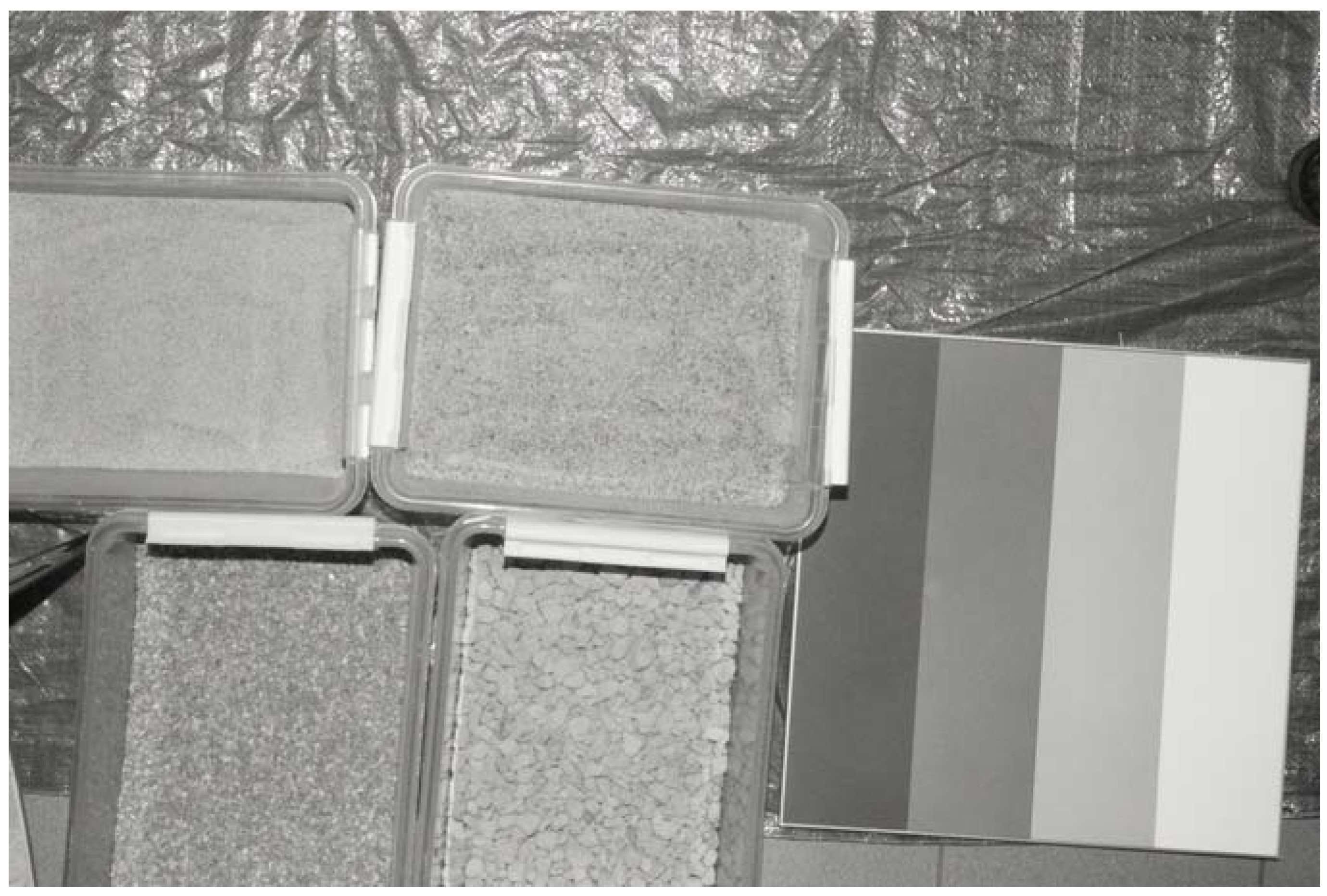
2.1. The Instruments and Measurements

2.2. Data Correction
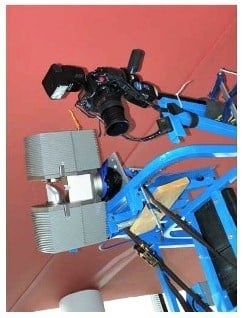
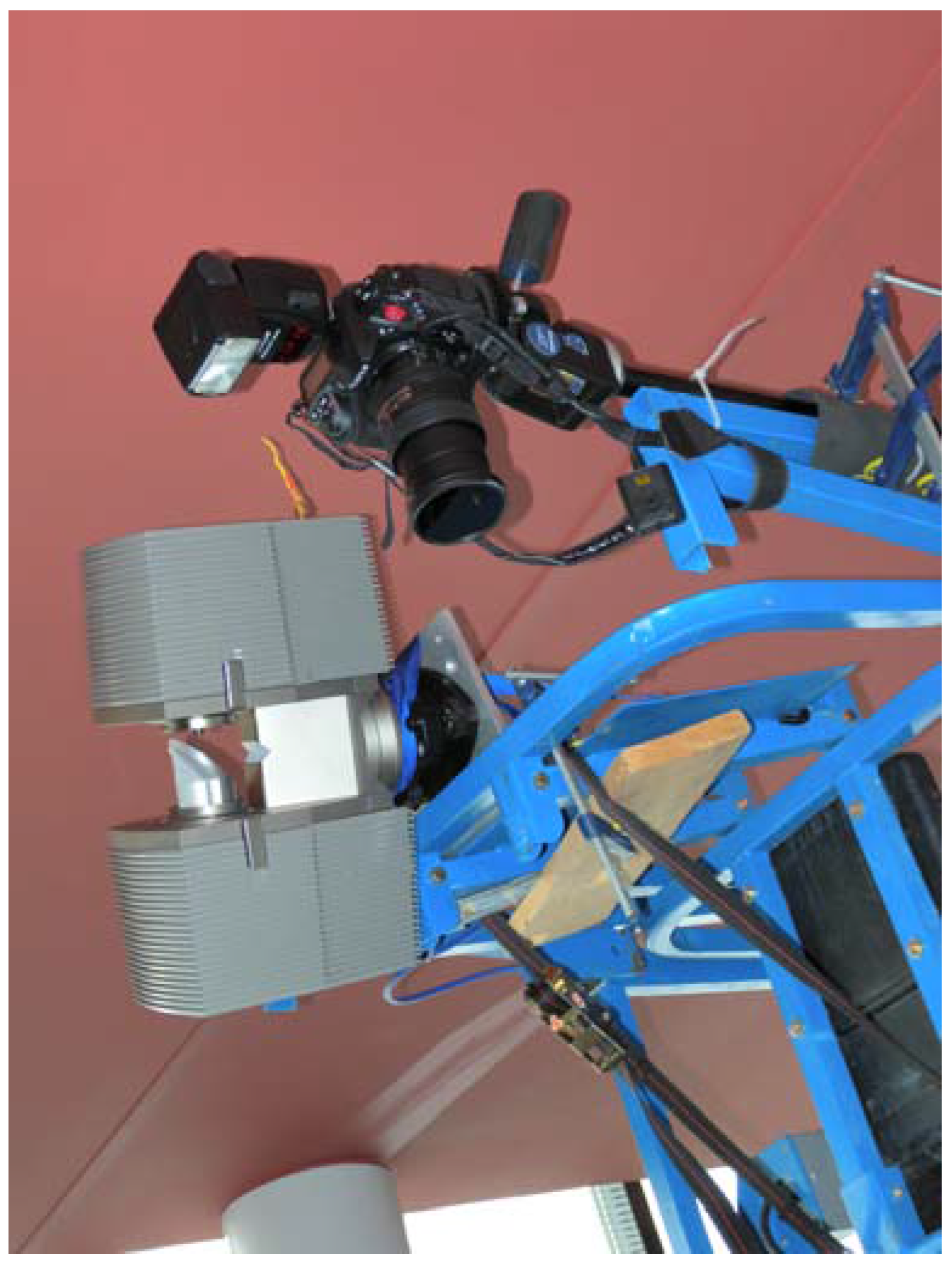
2.3. Near-Infrared Digital Camera
3. Results
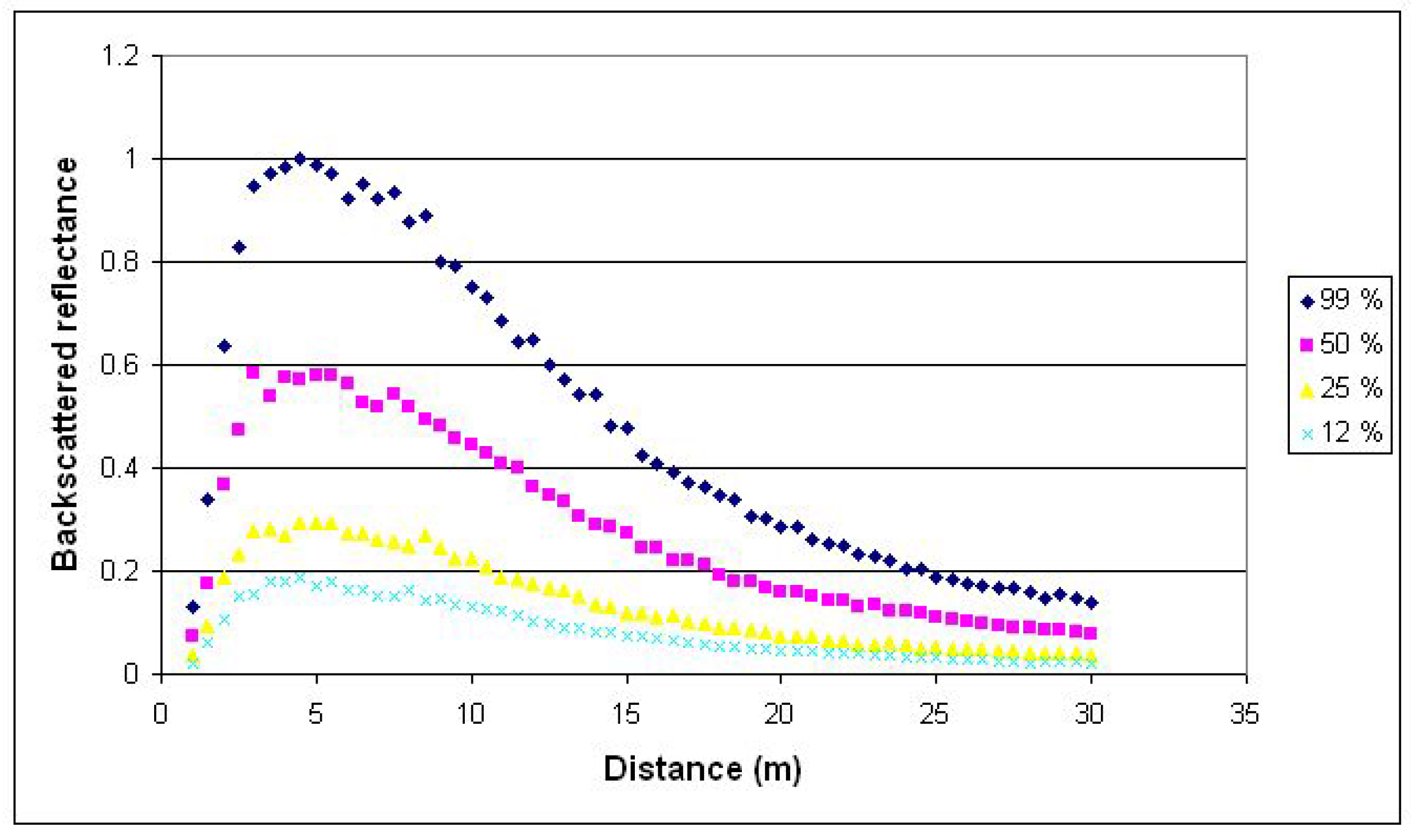
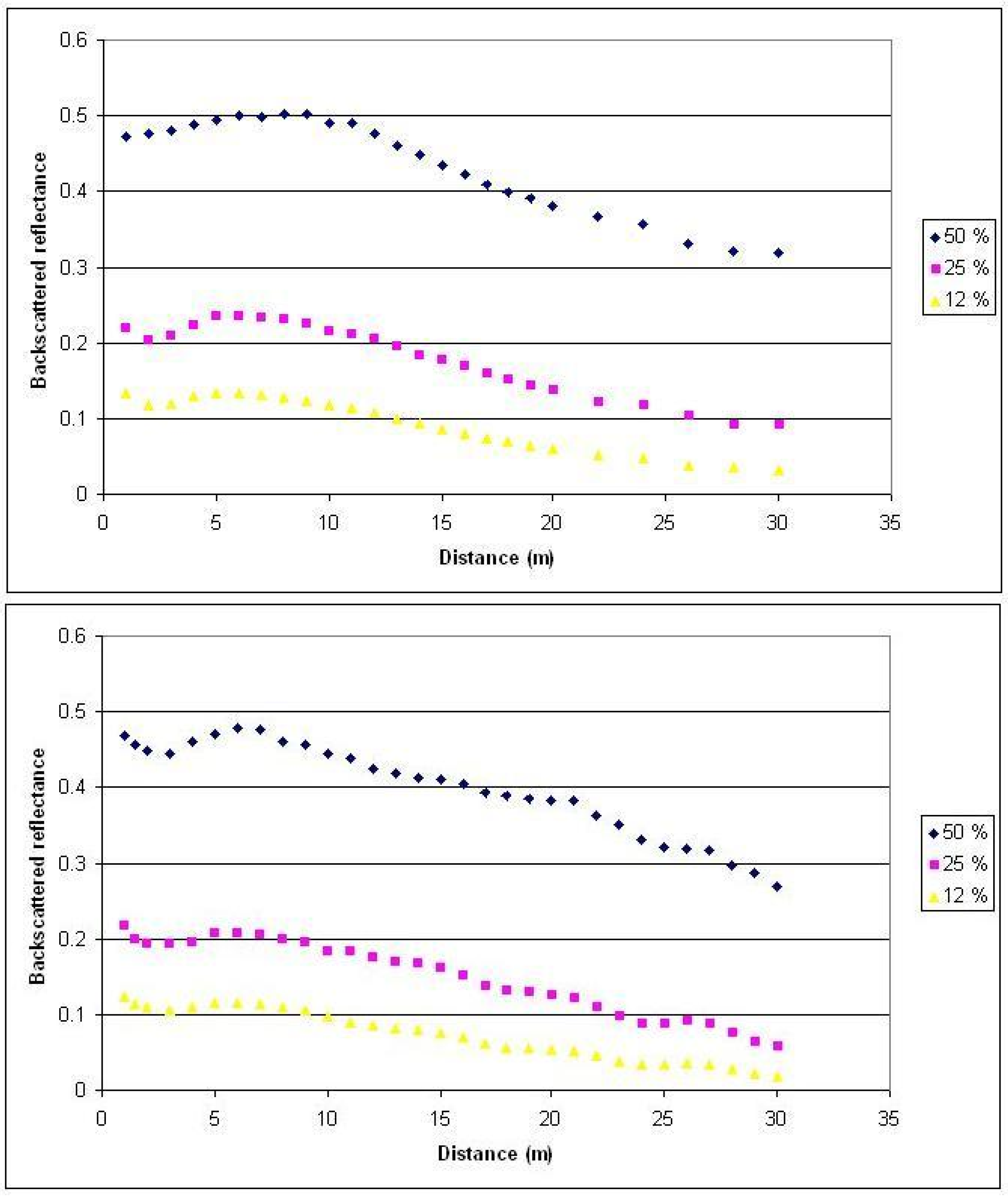
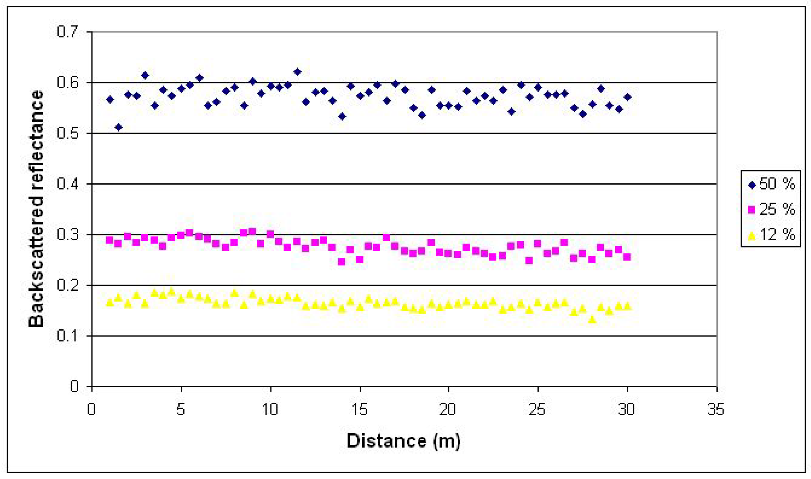
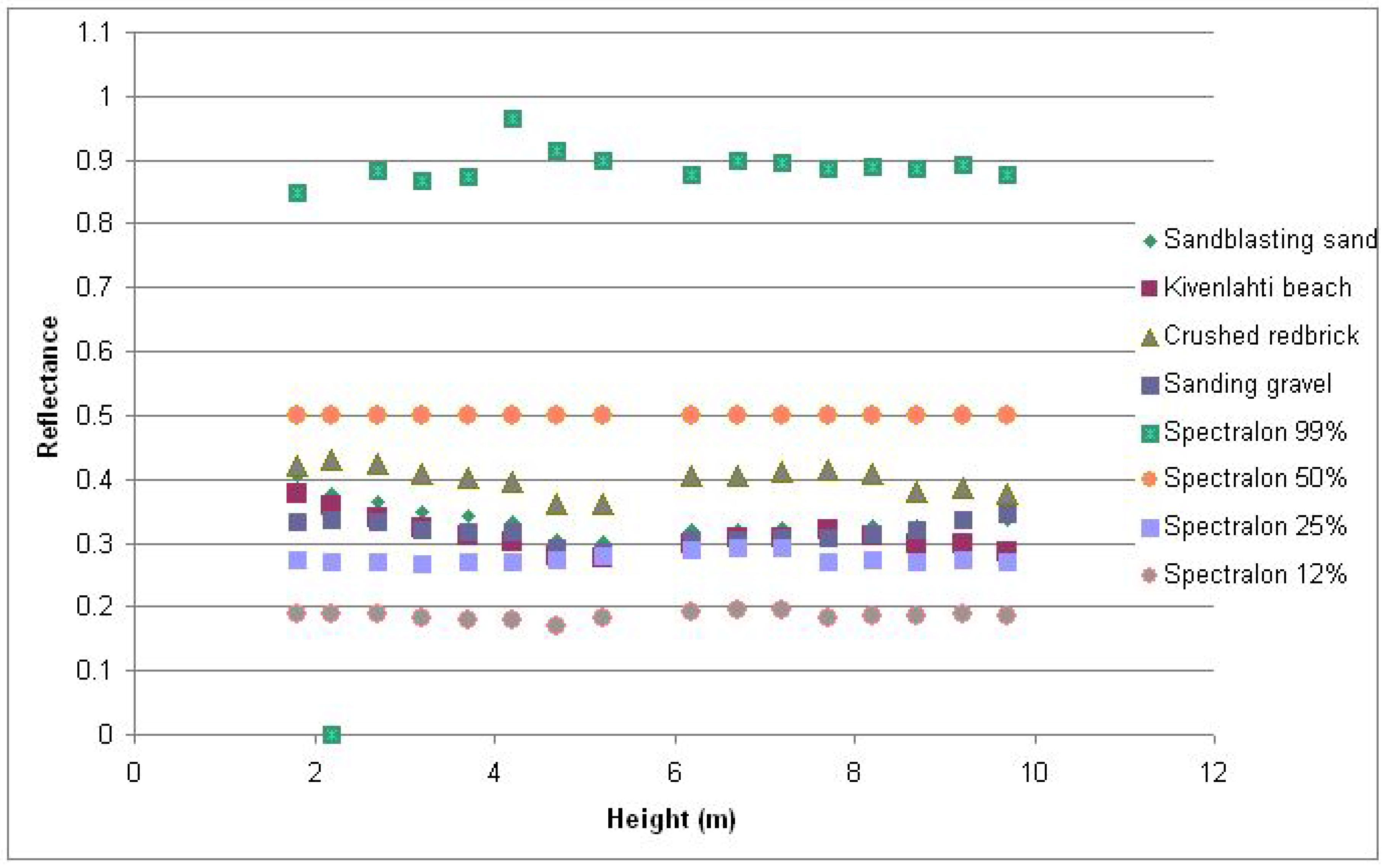
3.1. Distance Effects
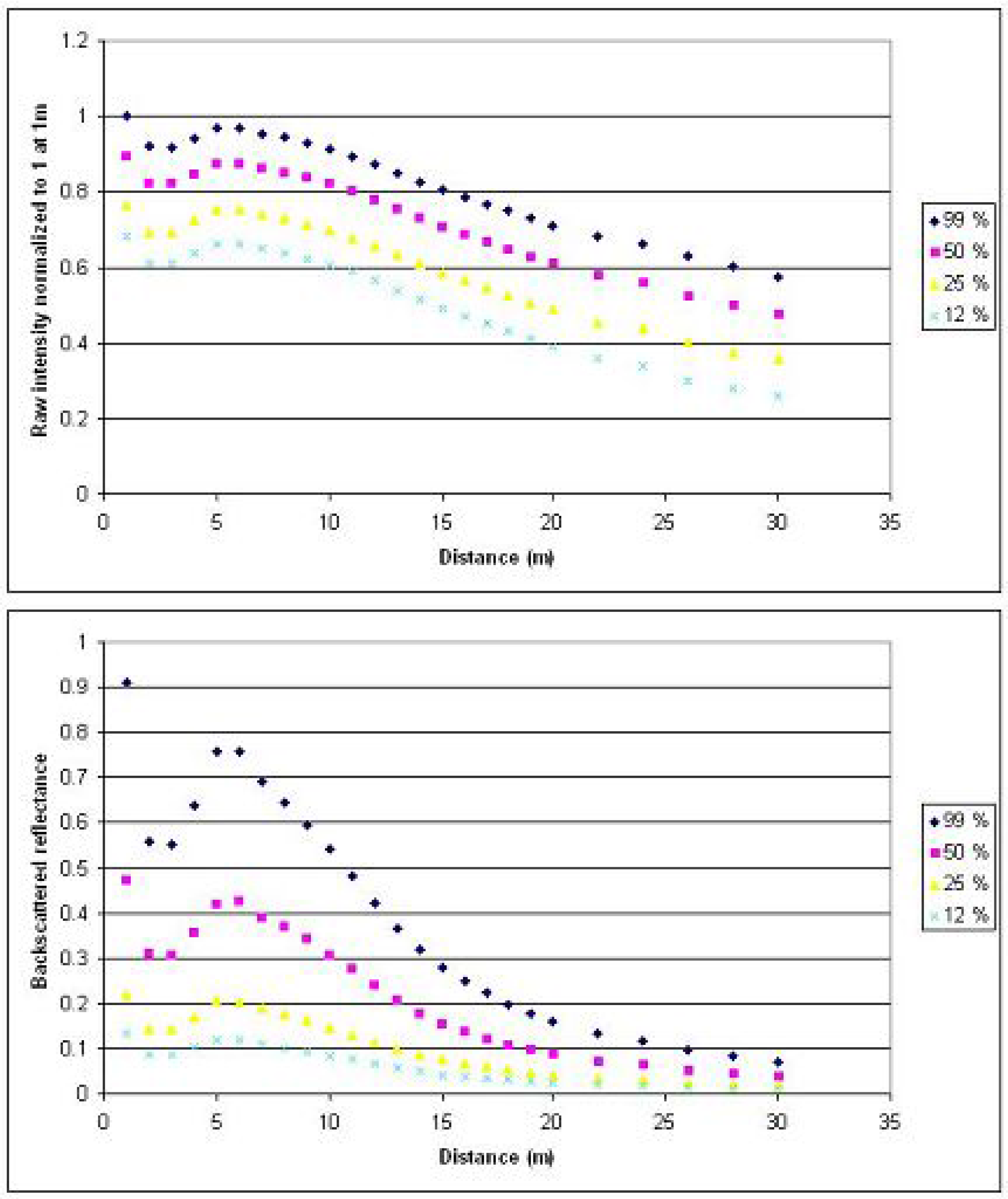

3.2. Calibration of Distance Effects

| 50% panel | 25% panel | 12% panel | |
| FARO 2007, 5 m | 0.494 ± 0.001 | 0.236 ± 0.001 | 0.134 ± 0.001 |
| FARO 2009, 5 m | 0.470 ± 0.002 | 0.207 ± 0.002 | 0.116 ± 0.002 |
| Leica 2009, 5 m | 0.59 ± 0.02 | 0.30 ± 0.02 | 0.17 ± 0.01 |
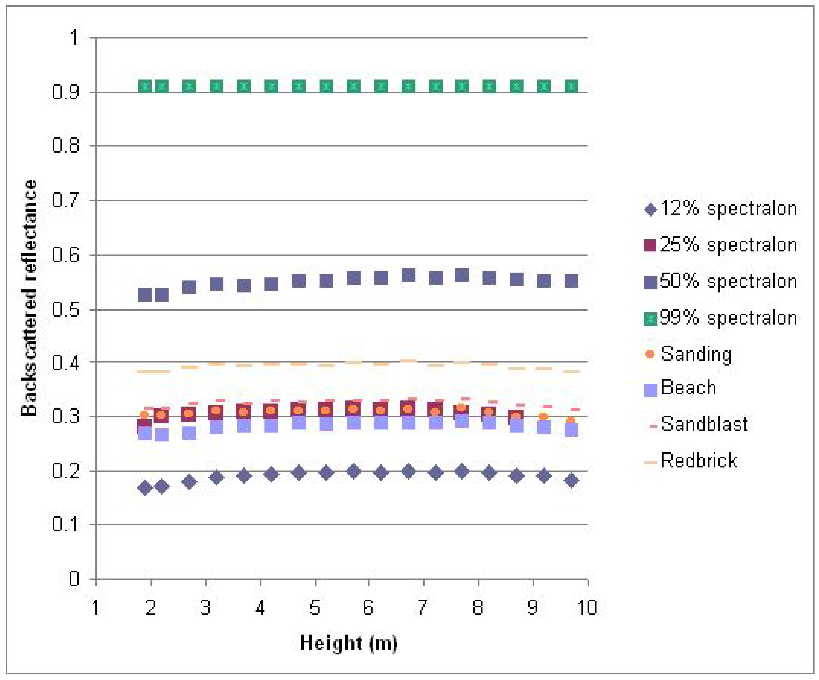
| FARO/Lift, 5.2 m | 0.553 ± 0.002 | 0.310 ± 0.002 | 0.196 ± 0.002 |
| Fuji/Lift, 5.2 m | - | 0.28 ± 0.09 | 0.18 ± 0.10 |


4. Conclusions
Acknowledgements
References and Notes
- Lichti, D.; Licht, M.G. Experiences with terrestrial laserscanner modelling and accuracy assessment. Int. Arch. Photogramm. Remote Sens. 2006, 36, 155–160. [Google Scholar]
- Lichti, D.D. Error modelling, calibration and analysis of an AM–CW terrestrial laser scanner system. ISPRS J. Photogramm. Remote Sens. 2007, 61, 307–324. [Google Scholar] [CrossRef]
- Danson, F.M.; Hetherington, D.; Morsdorf, F.; Koetz, B.; Allgöwer, B. Forest canopy gap fraction from terrestrial laser scanning. IEEE Trans. Geosci. Remote Sens. 2007, 4, 157–160. [Google Scholar] [CrossRef] [Green Version]
- Côté, J.-F.; Widlowski, J.-L.; Fournier, R.A.; Verstraete, M.M. The structural and radiative consistency of three-dimensional tree reconstructions from terrestrial lidar. Remote Sens. Environ. 2009, 113, 1067–1081. [Google Scholar] [CrossRef]
- Rosell Polo, J.R.; Sanz, R.; Llorens, J.; Arnó, J.; Escolà, A.; Ribes-Dasi, M.; Masip, J.; Camp, F.; Gràcia, F.; Solanelles, F.; Pallejà, T.; Val, L.; Planas, S.; Gil, E.; Palacín, J. A tractor-mounted scanning LIDAR for the non-destructive measurement of vegetative volume and surface area of tree-row plantations: a comparison with conventional destructive measurements. Biosyst. Eng. 2009, 102, 128–134. [Google Scholar] [CrossRef] [Green Version]
- Al-kheder, S.; Al-shawabkeh, Y.; Haala, N. Developing a documentation system for desert palaces in Jordan using 3D laser scanning and digital photogrammetry. J. Archaeol. Sci. 2009, 36, 537–546. [Google Scholar] [CrossRef]
- Entwistle, J.A.; McCaffrey, K.J.W.; Abrahams, P.W. Three-dimensional (3D) visualisation: the application of terrestrial laser scanning in the investigation of historical Scottish farming townships. J. Archaeol. Sci. 2009, 36, 860–866. [Google Scholar] [CrossRef]
- González-Aguilera, D.; Muñoz-Nieto, A.; Gómez-Lahoz, J.; Herrero-Pascual, J.; Gutierrez-Alonso, G. 3D digital surveying and modelling of cave geometry: application to paleolithic rock art. Sensors 2009, 9, 1108–1127. [Google Scholar] [CrossRef] [PubMed]
- Dunning, S.A.; Massey, C.I.; Rosser, N.I. Structural and geomorphological features of landslides in the Bhutan Himalaya derived from Terrestrial Laser Scanning. Geomorphology 2009, 103, 17–29. [Google Scholar] [CrossRef]
- Rabatel, A.; Deline, P.; Jaillet, S.; Ravanel, L. Rock falls in high-alpine rock walls quantified by terrestrial lidar measurements: A case study in the Mont Blanc area. Geophys. Res. Lett. 2008, 35, L10502. [Google Scholar] [CrossRef]
- Prokop, A. Assessing the applicability of terrestrial laser scanning for spatial snow depth measurements. Cold Regions Sci. Tech. 2008, 54, 155–163. [Google Scholar] [CrossRef]
- Schaffhauser, A.; Adams, M.; Fromm, R.; Jörg, P.; Luzi, G.; Noferini, L.; Sailer, R. Remote sensing based retrieval of snow cover properties. Cold Regions Sc. Tech. 2008, 54, 164–175. [Google Scholar] [CrossRef]
- Prokop, A.; Schirmer, M.; Rub, M.; Lehning, M.; Stocker, M. A comparison of measurement methods: terrestrial laser scanning, tachymetry and snow probing for the determination of the spatial snow-depth distribution on slopes. Ann. Glaciol. 2008, 49, 210–216. [Google Scholar] [CrossRef]
- Luzi, G.; Noferini, L.; Mecatti, D.; Macaluso, G.; Pieraccini, M.; Atzeni, C.; Schaffhauser, A.; Fromm, R.; Nagler, T. Using a ground-based SAR interferometer and a terrestrial laser scanner to monitor a snow-covered slope: Results from an experimental data collection in Tyrol (Austria). IEEE Trans. Geosci. Remote Sens. 2009, 47, 382–393. [Google Scholar] [CrossRef]
- von Hansen, W.; Gross, W.; Thoennessen, U. Line-based registration of terrestrial and airborne LIDAR data. Int. Arch. Photogramm. Remote Sens. 2008, 37, 161–166. [Google Scholar]
- Früh, C.; Zakhor, A. An automated method for large-scale, ground-based city model acquisition. Int. J. Comput. Vision 2004, 60, 5–24. [Google Scholar] [CrossRef]
- Stamos, I.; Allen, P.K. Geometry and texture recovery of scenes of large scale. Comput. Vision Image Understand. 2002, 88, 94–118. [Google Scholar] [CrossRef]
- Ikeuchi, K.; Oishi, T.; Takamatsu, J.; Sagawa, R.; Nakazawa, A.; Kurazume, R.; Nishino, K.; Kamakura, M.; Okamoto, Y. The Great Buddha project: digitally archiving, restoring, and analyzing cultural heritage objects. Int. J. Comput. Vision 2007, 75, 189–208. [Google Scholar] [CrossRef]
- Kukko, A.; Andrei, C.-O.; Salminen, V.-M.; Kaartinen, H.; Chen, Y.; Rönnholm, P.; Hyyppä, H.; Hyyppä, J.; Chen, R.; Haggrén, H.; Kosonen, I.; Capek, K. Road environment mapping system of the finnish geodetic institute - FGI roamer. Int. Arch. Photogramm. Remote Sens. 2007, 36, 241–247. [Google Scholar]
- Jaakkola, A.; Hyyppä, J.; Hyyppä, H.; Kukko, A. Retrieval algorithms for road surface modelling using laser-based mobile mapping. Sensors 2008, 8, 5238–5249. [Google Scholar] [CrossRef]
- Barber, D.M.; Mills, J.P. Vehicle based waveform laser scanning in a coastal environment. Int. Arch. Photogramm. Remote Sens. 2007, 36, C55. [Google Scholar]
- Alho, P.; Kukko, A.; Hyyppä, H.; Kaartinen, H.; Hyyppä, J.; Jaakkola, A. Mobile TLS application for fluvial studies. Geophys. Res. Abstr. 2009, 11, 7601. [Google Scholar]
- Amoureus, L.; Bomers, M.P.H.; Fuser, R.; Tosatto, M. Integration of LiDAR and terrestrial mobile mapping technology for the creation of a comprehensive road cadastre. Int. Arch. Photogramm. Remote Sens. 2007, 36, C55. [Google Scholar]
- Coren, F.; Sterzai, P. Radiometric correction in laser scanning. Int. J. Remote Sens. 2006, 27, 3097–3104. [Google Scholar] [CrossRef]
- Höfle, B.; Pfeifer, N. Correction of laser scanning intensity data: data and model-driver approaches. ISPRS J. Photogramm. Remote Sens. 2007, 62, 415–433. [Google Scholar] [CrossRef]
- Kaasalainen, S.; Kukko, A.; Lindroos, T.; Litkey, P.; Kaartinen, H.; Hyyppä, J.; Ahokas, E. Brightness measurements and calibration with airborne and terrestrial laser scanners. IEEE Trans. Geosci. Remote Sens. 2008, 46, 528–534. [Google Scholar] [CrossRef]
- Kaasalainen, S.; Kaartinen, H.; Kukko, A. Snow cover change detection with laser scanning range and brightness measurements. EARSeL eProc. 2008, 7, 133–141. [Google Scholar]
- Kang, Z.; Li, J.; Zhang, L.; Zhao, Q.; Zlatanova, S. Automatic registration of terrestrial laser scanning point clouds using Panoramic Reflectance Images. Sensors 2009, 9, 2621–2646. [Google Scholar] [CrossRef] [PubMed]
- González-Aguilera, D.; Rodríguez-Gonzálvez, P.; Gómez-Lahoz, J. An automatic procedure for co-registration of terrestrial laser scanners and digital cameras. ISPRS J. Photogramm. Remote Sens. 2009. in Press. [Google Scholar]
- Pesci, A.; Teza, G. Terrestrial laser scanner and retro-reflective targets: An experiment for anomalous effects investigation. Int. J. Remote Sens. 2008, 29, 5749–5765. [Google Scholar] [CrossRef]
- Jaakkola, A.; Kaasalainen, S.; Hyyppä, J.; Akujärvi, A.; Niittymäki, H. Radiometric calibration of intensity images of SwissRanger SR-3000 range camera. Photogramm. J. Finland 2008, 21, 16–25. [Google Scholar]
- Pfeifer, N.; Höfle, B.; Briese, C.; Rutzinger, M.; Haring, A. Analysis of the backscattered energy in terrestrial laser scanning data. Int. Arch. Photogramm. Remote Sens. 2008, 37, 1045–1052. [Google Scholar]
- Wagner, W.; Hyyppä, J.; Ullrich, A.; Lehner, H.; Briese, C.; Kaasalainen, S. Radiometric calibration of full-waveform small-footprint airborne laser scanners. Int. Arch. Photogramm. Remote Sens. 2008, 37, 163–168. [Google Scholar]
- Kaasalainen, S.; Hyyppä, H.; Kukko, A.; Litkey, P.; Ahokas, E.; Hyyppä, J.; Lehner, H.; Jaakkola, A.; Suomalainen, J.; Akujärvi, A.; Kaasalainen, M.; Pyysalo, U. Radiometric Calibration of LIDAR Intensity With Commercially Available Reference Targets. IEEE Trans. Geosci. Remote Sens. 2009, 47, 588–598. [Google Scholar] [CrossRef]
- Vain, A.; Kaasalainen, S.; Pyysalo, U.; Krooks, A.; Litkey, P. Use of naturally available reference targets to calibrate airborne laser scanning intensity data. Sensors 2009, 9, 2780–2796. [Google Scholar] [CrossRef] [PubMed]
© 2009 by the authors; licensee Molecular Diversity Preservation International, Basel, Switzerland. This article is an open-access article distributed under the terms and conditions of the Creative Commons Attribution license (http://creativecommons.org/licenses/by/3.0/).
Share and Cite
Kaasalainen, S.; Krooks, A.; Kukko, A.; Kaartinen, H. Radiometric Calibration of Terrestrial Laser Scanners with External Reference Targets. Remote Sens. 2009, 1, 144-158. https://doi.org/10.3390/rs1030144
Kaasalainen S, Krooks A, Kukko A, Kaartinen H. Radiometric Calibration of Terrestrial Laser Scanners with External Reference Targets. Remote Sensing. 2009; 1(3):144-158. https://doi.org/10.3390/rs1030144
Chicago/Turabian StyleKaasalainen, Sanna, Anssi Krooks, Antero Kukko, and Harri Kaartinen. 2009. "Radiometric Calibration of Terrestrial Laser Scanners with External Reference Targets" Remote Sensing 1, no. 3: 144-158. https://doi.org/10.3390/rs1030144