1. Introduction
There is great interest in proximal and remote sensing methods for monitoring leaf area, cover and biomass in forests because of potential impacts of large scale of deforestation and reforestation on the Earth’s carbon cycle [
1], and the likely wide-scale impacts that on-going climate change is in-turn predicted to have on the world’s forests [
2] including Mediterranean regions [
3]. The amount of foliage in a forest’s canopy is a key indicator of its carbon and water balance, because the canopy is the main interface through which carbon is sequestered into biomass via photosynthesis and which water is lost to the atmosphere via evaporation. Spectral indices, such as normalized-difference vegetation index, are strongly correlated with chlorophyll or canopy nitrogen [
4,
5,
6] making it possible to remotely-sense canopy metrics such as leaf area and cover, but ground-based methods for quantifying the distribution and abundance of foliage are essential for calibrating spectral indices. However, in addition to being time-consuming and tedious [
7], direct measurement of canopy foliage is difficult, expensive and potentially hazardous owing to the need for tree-felling, and site access is often poor due to difficult terrain [
8,
9,
10]. Consequently indirect measurements of leaf area index (
LAI, the one-sided area of foliage per unit ground area [
11]) and cover (the fraction of ground shaded by the vertical projection of tree crowns [
12]) are often used as proxies for actual canopy leaf area and biomass.
This paper brings to the attention of the remote sensing community a new method, digital cover photography (DCP), for estimating both crown cover and
LAI, in addition to other canopy traits [
13,
14,
15]. This method has been successfully used to calibrate remotely sensed vegetation indices in two recent studies [
16,
17]. The method involves collecting vertically oriented digital photographic images with a narrow field-of-view (typically 30°) and dividing the total zenithal gap fraction into large, mainly between-crown, and small, mainly within-crown, gaps. DCP has the advantages that it can be routinely applied during normal working hours (unlike fisheye photography or the Licor
LAI-2000); sky luminance is more even, facilitating pixel classification; the narrow viewing angle and rectangular shape of the images is better suited to small rectangular experimental plots than the large circular footprint of hemispherical sensors; and the images are much higher resolution than fisheye images and, thus, they are less sensitive to photographic exposure and should provide a more accurate measurement of the gap fraction at the zenith. This paper briefly summarizes the theory and practice of DCP, and compares it to more established fisheye photography methods. Unlike circular fisheye photography, which has a long history of application in forestry and plant ecology [
18] and has been the subject of several reviews [
8,
9,
10,
19,
20,
21,
22], some aimed at the remote sensing community [
23,
24,
25,
26], DCP has not been dealt with in any previous reviews.
The objective of this paper is to conduct a thorough technical appraisal of the factors that may affect the results obtained using either digital point-and-shoot cameras or single-lens-reflex (DSLR) cameras. We test the effect of camera settings including file compression, image size and ISO (International Standards Organization) equivalence, as well as threshold selection during image processing, on the results obtained from DCP and fisheye photography using both types of camera. This study is the first technical appraisal of DCP but some previous studies have compared different models of point-and-shoot camera as well as examining the impact of image size or file compression [
27,
28,
29] on results from fisheye photography. Frazer
et al. [
27] compared film photography with the 2.1 megapixel Coolpix 950, while Inoue
et al. [
28] compared the 3.1 megapixel Coolpix 990 with the early model 1.2 megapixel Coolpix 900. Englund
et al. [
29] tested the effect of image quality using the Coolpix 950. These researchers discovered that little or no difference exists between TIFF and JPEG images from the same camera, but that image size can influence estimates of leaf area although the direction of the change was not consistent between studies. None of the above researchers studied the effect of the camera’s ISO equivalence on estimates of cover or
LAI. ISO is a measure of the sensitivity of film to light (film with a smaller ISO number is less sensitive) but also quantifies the relative sensitivity of CDD (charge coupled device) or CMOS (complementary metal-oxide semiconductor) sensors to light. The ability to increase a digital camera’s ISO equivalence without having to change film is another advantage of digital photography over film photography. However, increasing the ISO equivalence also decreases a camera’s signal-to-noise ratio, especially for point-and-shoot cameras with small pixels. The Nikon Coolpix 4500 was the last Coolpix model to use the FC-E8 fisheye converter but is now discontinued. Since then DSLR cameras have become much more affordable and digital camera resolution has increased greatly: 6 to 12 megapixel cameras that produce unprocessed RAW images are now cheaply available. For example, the Nikon D80 digital single-lens-reflex (DLSR) and Coolpix 4500 have similar luminance noise at ISO 100 but noise in the 4500 at ISO 800 (its largest ISO) is more than three times that of the D80 at ISO 1,600 [
30]; the pixels on the CCD of the 4500 are approximately one-quarter the area of those on the D80. How these factors will affect estimates using finer resolution images collected with better quality optics in DLSR cameras is unknown. Lenses available for DSLR cameras will have superior optical quality to the built-in zoom lenses and lens converters of the Coolpix cameras. We specifically tested the hypotheses that:
File compression would have no effect on estimates of canopy structure from either photographic method.
Increasing ISO would alter estimates of canopy structure from DCP, especially using the Coolpix 4500.
Changing the size of images would change estimates of canopy structure from the DSLR camera, and that smaller images would give similar estimates to those from the lower-resolution Coolpix 4500.
We contrast the performance of DCP with that of fisheye photography. We also evaluated the sensitivity of DCP to variations in threshold selection during image classification. Finally, we discuss the application of DCP to calibration and testing of remotely sensed forest metrics.
2. Materials and Methods
2.1. Introduction to Digital Cover Photography (DCP)
Unlike fisheye photography, DCP uses a narrow field-of-view (FOV) lens aimed at the zenith (
Figure 1) and achieves very-fine spatial resolution [
14,
15]. We use a 70 mm equivalent focal-length lens (in 35 mm format) to obtain an approximately 30° FOV. This provides a compromise between vertical FOV and adequate spatial sampling, and is also comparable with the FOV of the first ring of the Licor
LAI-2000, which was used by Kucharik
et al. [
9] to measure cover. Each individual image captures a small area of the canopy (the exact area depends on the height of the vegetation); the total area sampled is determined by the number and extent of images collected. Circular fisheye images contain the entire 180° hemisphere in a circle that occupies about half the pixels inside a rectangular image, while full-frame fisheye images have a 180° FOV across the diagonal (
Figure 1), roughly doubling image resolution. These latter two image types were recently compared with DCP by Macfarlane
et al. [
14]. Whereas fisheye methods attempt to use the variation in gap fraction with zenith angle to determine
LAI [
19], DCP is a single (or restricted) view-angle method.
Figure 1.
Comparison of wide-angle fisheye and 57° photographic images with narrow FOV cover images.
Figure 1.
Comparison of wide-angle fisheye and 57° photographic images with narrow FOV cover images.
Essentially, the digital cover photography method divides canopy gaps into those where Beer’s law applies (within-crown) and those where it does not (between-crown). A similar approach was taken by Song and Band [
31] to model photosynthetically active radiation under discrete forest canopies. An example of a cover image that has been classified into canopy and sky pixels, with the sky pixels further classified into large, between-canopy gaps and small, within-canopy gaps, is given in
Figure 2. Many within-crown canopy gaps are not detectable at all in low-resolution fisheye images.
Crown cover (
fc) is defined as the fraction of pixels that do not lie in between-crown gaps and is equivalent to Nilson’s [
32] “canopy closure”. Foliage cover (
ff, also known as foliage projective cover [
33]) is the fraction of pixels not in any gaps,
i.e., foliage and wood. Based on previous studies [
13,
14,
15] we classify gaps larger than 1.3% of the total image area as between-canopy gaps. Note that we use the term “crown cover” to describe the fractional ground cover of the vertical projection of solid crowns that may or may not overlap, and which can not exceed one. We refer the reader to articles by Walker and Tunstall [
12] and Jennings
et al. [
34] for good discussions of the sometimes confusing terminology relating to cover measurement in forest vegetation.
Figure 2.
Example of a cover image that has been classified into canopy (black), small within crown gaps pixels (white) and large between-crown gaps (grey). Crown cover (0.51) is the fractional cover of black+white pixels. Foliage cover (0.29) is the fractional cover of black pixels. Crown porosity (Equation 1) is the ratio of white to black+white pixels (0.44).
In addition to being a very simple, rapid and accurate method for measuring crown and foliage cover in forests, DCP estimates a suite of other variables of interest: crown porosity (
Φ, proportion of sky within crown envelopes, Equation 1),
LAI (Equation 2) and zenithal clumping index (
Ω(0), Equation 3). Note that our Equation 2 is quite different to Sprintsin
et al. [
35] Equation 5, which includes only between-crown gaps in the logarithmic term of Beer’s law and then lumps together clumping effects and within crown gaps in the empirically derived value of
k. In open forests where crowns rarely overlap, crown cover and
LAI will be linearly related if
Φ and
k are unchanged.
The concept of crown porosity, derived from vertical gap-fraction measurements, was pioneered by Kucharik
et al. [
9]; in North American forests, Kucharik
et al. [
9] estimated
Φ of 0.12 in stands of black spruce, 0.20 in jack pine and 0.29 in aspen. Using DCP, we have estimated
Φ to range from 0.11–0.15 for forest of
Eucalyptus diversicolor and rapidly growing stands of
E. marginata, to as much as 0.27–0.39 for woodlands of
E. accedens and
E. salmonophloia (
Table 1). Natural forest of
E. marginata is variable with
Φ ranging from 0.14 to 0.34 (
Table 1).
Table 1.
Estimates of crown porosity (Φ) in eucalypt forest obtained from DCP.
Table 1.
Estimates of crown porosity (Φ) in eucalypt forest obtained from DCP.
| Forest | Source | Φ |
|---|
| E. salmonophloia woodland - Quairading | Unpublished data | 0.27–0.39 |
| E. accedens woodland - Wandoo Nat. Park | [16] | 0.27–0.34 |
| E. marginata forest - Dwellingup | Unpublished data | 0.19–0.34 |
| E. marginata forest - Bates | Unpublished data | 0.14 |
| Regrowth E. marginata forest - Dwellingup (Huntly) | Unpublished data | 0.18 |
| Old-growth E. marginata forest - Dwellingup (Huntly) | Unpublished data | 0.27 |
| E. marginata forest - Mundaring | [16] | 0.14–0.22 |
| E. resinifera plantation - Mundaring | [16] | 0.15–0.19 |
| E. diversicolor - Pemberton | Unpublished data | 0.15–0.25 |
| E. diversicolor - Dwellingup | Unpublished data | 0.14–0.15 |
| E. marginata rehab - Dwellingup (thin–burn trial) | [14] | 0.11–0.15 |
| E. marginata rehab - Dwellingup (Bleby) | [15] | 0.13 |
| E. marginata rehab - Dwellingup (Lewis) | Unpublished data | 0.11 |
Like fisheye sensors, estimation of foliage cover and
LAI from DCP is subject to errors resulting from the contribution of woody canopy elements to canopy cover. If
k is derived empirically from independent measurements of cover and
LAI, then
k effectively also corrects for woody area. The greatest disadvantage of DCP is the need to know, or estimate,
k in order to estimate
LAI from measurements of cover. If measurement of cover only is sufficient then this is no longer a disadvantage. Otherwise,
k must be estimated from knowledge of the leaf inclination angle distribution or estimated empirically by comparing measurements of crown cover and porosity with
LAI estimated from destructive harvesting or other suitable reference methods. We refer the reader to Ryu
et al. [
36] for a recent summary of methods used to estimate leaf inclination angles, including the photographic method developed by those authors. In theory the greatest advantage of fisheye and other multiple viewing-angle methods is the estimation of
LAI from measurement of the gap fraction at multiple zenith angles, although in practice this advantage is seldom realized owing to the strong dependence of the calculated
LAI and foliage inclination angle distribution on foliage clumping [
13,
14,
15,
32].
In the following sections we describe our approach to testing our hypotheses, and provide the technical detail of how DCP is implemented in the field and image processing and analysis.
2.2. Field Sites and Field Methods
We tested the effect of JPEG compression, image size and type of camera on estimates of canopy structure at seven eucalypt forest sites in south-western Australia. The area has a Mediterranean-type climate characterized by mild winters and hot, dry summers. The overstorey of the forest was dominated by tall (30 m) karri trees (
Eucalyptus diversicolor) at one site, medium height (15–20 m) jarrah (
E. marginata) and marri (
Corymbia calophylla) trees at three sites, and shorter (10–15 m) wandoo (
E. wandoo) and powderbark wandoo (
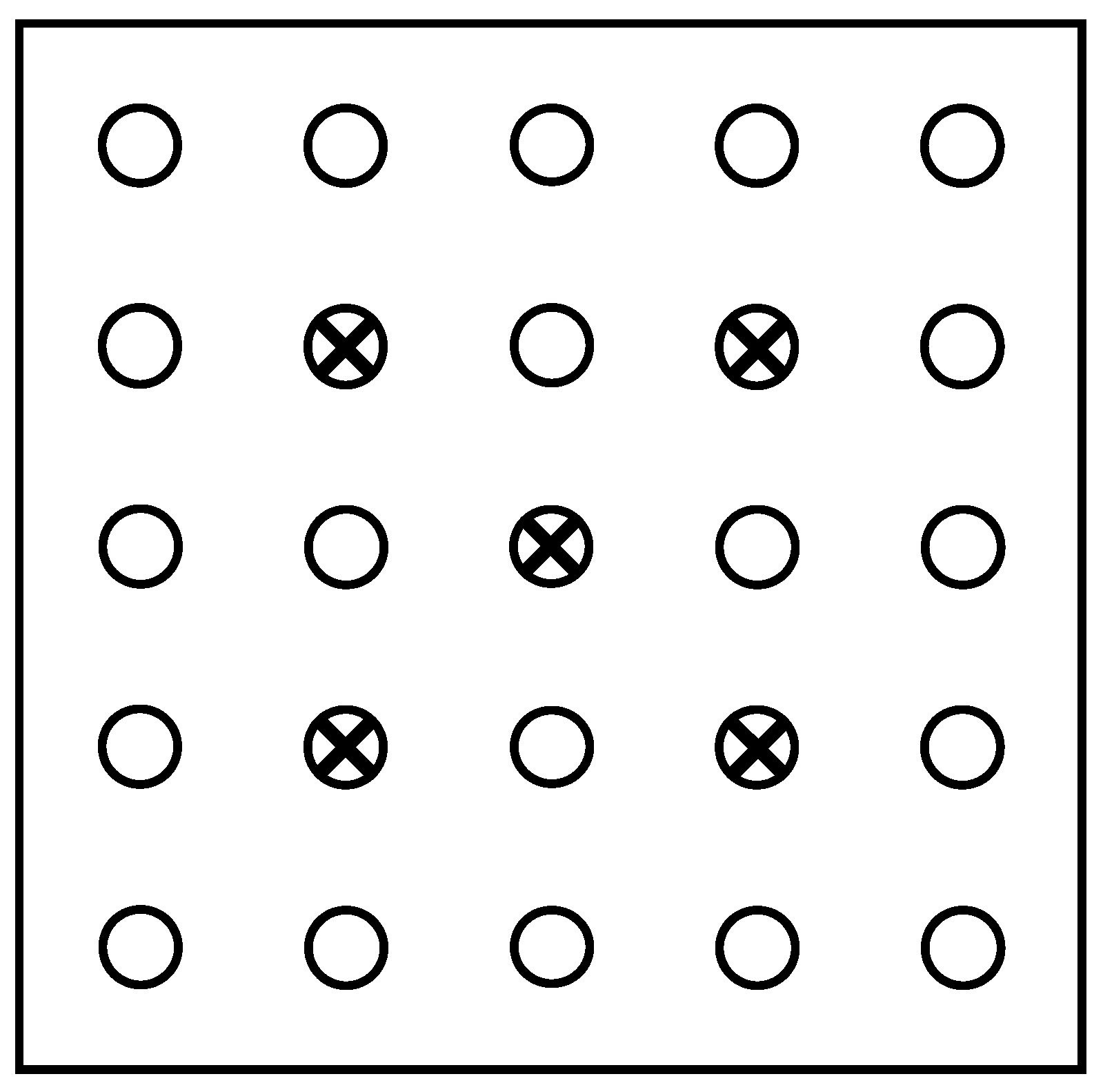
E. accedens) at three sites. At each site a 40 m × 40 m plot was established on flat or gentle sloping terrain. We collected cover images at 25 sample points, and fisheye images at five sample points (
Figure 3) using both the Nikon D80 (henceforth referred to as the D80) and the Nikon Coolpix 4500 (henceforth referred to as the 4500).
Figure 3.
Indicative sampling positions for fisheye photography (crosses) and cover images (circles) in the sample plots. Cover images are spaced 10 m apart but sample outside the 40 m × 40 m, effectively sampling an area of 50 m × 50 m, represented by the square box.
Figure 3.
Indicative sampling positions for fisheye photography (crosses) and cover images (circles) in the sample plots. Cover images are spaced 10 m apart but sample outside the 40 m × 40 m, effectively sampling an area of 50 m × 50 m, represented by the square box.
Cover images were collected late in the day using an AF Nikkor 50 mm 1:1.8 D lens on the D80 or by setting the 4500 to F2 lens setting. These yielded very similar fields of view for the two cameras despite their different aspect ratios (3:2 for the D80 and 4:3 for the 4500). Full-frame fisheye images were collected at dusk, when background sky illumination is most even, using an AF Fisheye Nikkor 10.5 mm 1:2.8 G lens fitted to the D80 or with a FC-E8 fisheye converter fitted to the 4500, which was set to F2 lens mode. These both yielded images with an approximately 180° FOV across the diagonal.
All cover images were taken with an aperture setting of
f9.6 with the cameras set to ISO 100, Aperture Priority mode, auto-focus and auto-exposure. Full-frame fisheye images were taken with the cameras set to auto-focus and Manual mode with aperture of
f9.6, and with the shutter speed adjusted so that clear sky was over-exposed by one stop [
37,
38]. Using the D80 we compared uncompressed image files (NEF) with JPEG compressed files and we compared JPEG files of varying size or resolution, 10.0, 5.6 and 2.5 megapixels (
Table 1). NEF is Nikon’s proprietary RAW file format. Photos taken with the 4500 were JPEG images with a resolution of 3.9 megapixels (
Table 2); we compared these to an average of the small and medium JPEG from the D80 to compare the two cameras. JPEG images were FINE quality. We tested the effect of ISO setting on estimates of canopy structure from DCP by taking photographs directly beneath the canopies of 20 trees that varied in height, leaf size, shape and angle, and crown density. We used ISO settings of 100, 200, 400, 800 and 1,600 for the D80 but ISO 1,600 was not available on the 4500; aperture was fixed at
f8.0 for the D80 and
f7.7 for the 4500. The cameras were set to auto-exposure so that shutter speed would automatically compensate for changes in ISO. We took photographs in clear sky conditions with little wind to obtain adequate shutter speeds to “freeze” any foliage movement at small ISO settings.
Table 2.
List of image types collected at each forest site, using both cover and full-frame fisheye photography.
Table 2.
List of image types collected at each forest site, using both cover and full-frame fisheye photography.
| Camera | File compression | Image dimensions | Image size (megapixels) |
|---|
| D80 | none/NEF | 3,872 × 2,592 | 10.0 |
| D80 | JPEG (large) | 3,872 × 2,592 | 10.0 |
| D80 | JPEG (medium) | 2,896 × 1,944 | 5.6 |
| D80 | JPEG (small) | 1,936 × 1,296 | 2.5 |
| Coolpix 4500 | JPEG | 2,272 × 1,704 | 3.9 |
2.3. Image Processing and Analysis
All canopy image analyses were performed using WinSCANOPY 2006a (Regent Instruments, Ste. Foy, Quebec) as described by Macfarlane
et al. [
14] with one exception: images from the ISO study were not converted to black-and-white using the automatic threshold routine in WinSCANOPY but were instead converted to black-and-white using a threshold set to 150. We did this to eliminate any variation in threshold from the evaluation of ISO changes on canopy structure. The ISO images were collected at exactly the same place and time with exactly the same automatic exposure; hence, they should require the same threshold for conversion to B&W. A threshold of 150 was selected as being typical of well-exposed cover images; see for example
Figure 7a in [
17]. Prior to analysis, NEF images were converted to 8-bit TIFF images using Nikon’s Picture Project 1.7 software supplied with the D80.
From cover images we estimated
ff,
fc,
Φ (Equation 2),
LAI (Equation 3) and
Ω(0) (Equation 4) after Macfarlane
et al. [
14,
15]. This analysis corrects for foliage clumping using a simple gap-removal process: gaps larger than 1.3% of the total image area were classified as large gaps and not included in the calculation of crown porosity (the ‘within-crown’ gap fraction to which Beer’s Law is applied) [
13,
14,
15,
16]. The blue channel of the sharpened (medium) RGB images was analyzed and sky pixels were separated from canopy pixels using a threshold brightness value that was automatically determined by algorithms within the software. No corrections were made for woody area for any of the photographic methods; however, the DCP method has been calibrated against
LAI estimated from destructive sampling in this vegetation type [
14,
15] and we refer to estimates from this method as
LAI. We also refer to estimates from fisheye photography as
LAI to avoid confusion. For calculation of
LAI from cover images we assumed a light extinction coefficient (
k) at the zenith of 0.5, which has provided accurate estimates of
LAI in this vegetation in previous studies [
14,
15].
From fisheye images we estimated canopy openness,
LAI, mean leaf inclination angle and foliage clumping index using WinSCANOPY. The blue channel of all RGB images was sharpened (medium) and analyzed using a sky grid comprising of seven zenith rings from 0 to 70° and eight azimuth regions.
LAI from fisheye images was estimated using the generalized
LAI-2000 method [
39] for unmodified gap fraction data (linear method) and log-transformed gap fraction data. We have previously found the log method [
40] to give the best estimates of
LAI from fisheye images in this forest type. A mean clumping index was calculated as the ratio of
LAI from the linear- to the log-averaging method [
41]. We also calculated
LAI using the Chen and Cihlar [
42] gap-removal method which is also implemented in WinSCANOPY. The ellipsoidal method [
43] was used to calculate the mean leaf inclination angle from log-averaged gap fractions. WinSCANOPY also calculated openness (the fraction of visible open sky across the hemisphere).
2.4. Threshold for Image Segmentation
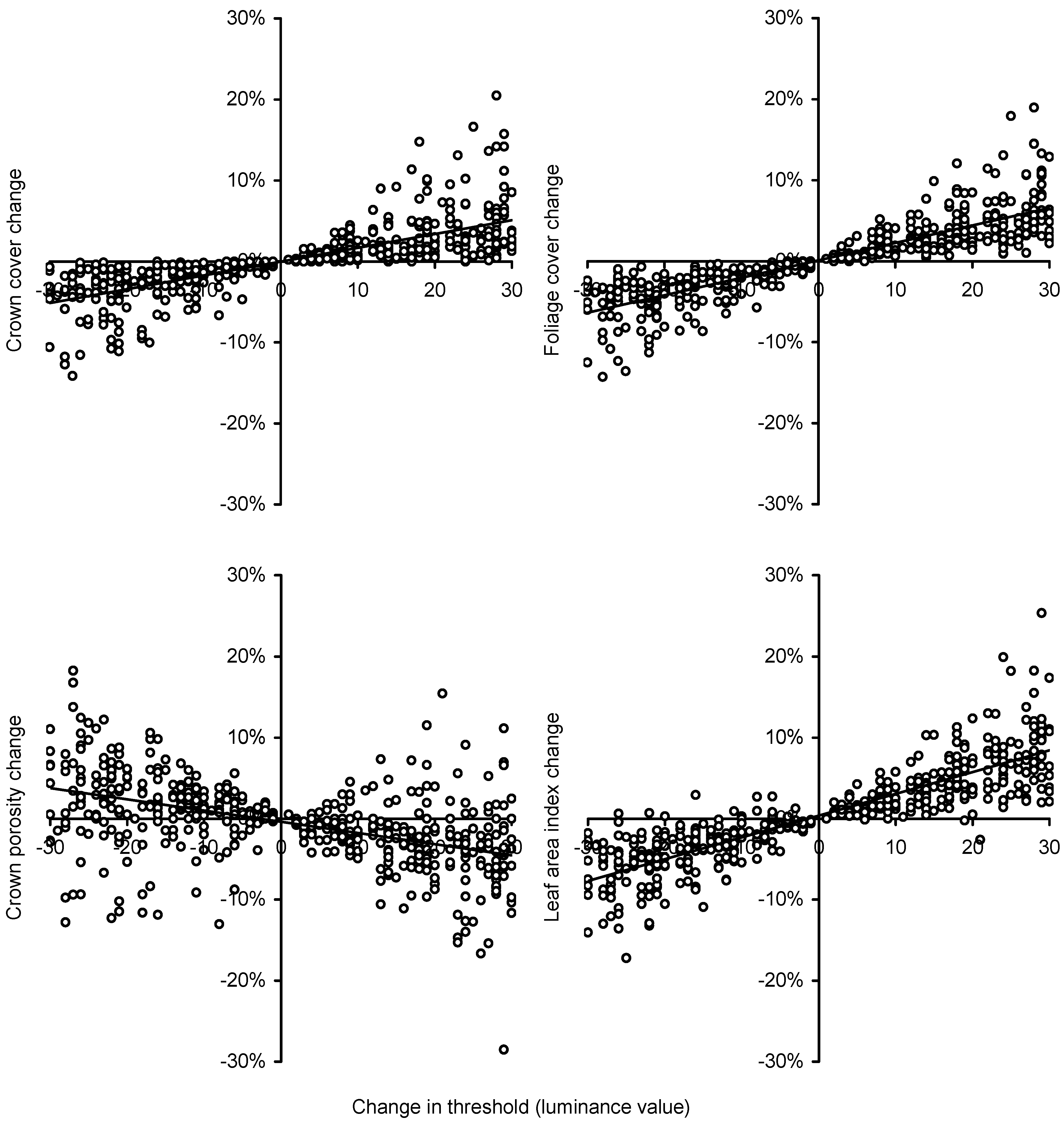
To test the sensitivity of DCP to choice of threshold during image segmentation we selected 88 images with a range of cover and reanalyzed them with fixed luminance thresholds ranging from 70 to 180. The difference in threshold from the automatic value to the manually fixed value was calculated (only data for which the luminance differed by no more than 30 were used) and the calculated covers, porosities and LAIs were compared to those from the images that had been analyzed using automatic threshold selection by WinSCANOPY. We avoided using images with unusually high or low threshold values that would have resulted in the threshold luminance value being near the peak values for sky or foliage.
2.5. Statistical Analyses
We compared the effect of site (first factor) and image compression, ISO setting, file size or camera (second factor) on estimated canopy characteristics using two-way ANOVA (sequential sum of squares), with R version 2.6.2 [
44]. No interactions between site and the second factor were observed; hence, the interaction term was removed from all analyses. The effect of image size was tested by comparing the three D80 JPEG files, large, medium and small. The effect of image compression was tested by comparing the D80 NEF and D80 large JPEG. And the effect of camera type was tested by comparing the 4500 JPEG with an average of the results from the small and medium D80 JPEG files.
2.6. Lens Calibration
Many fisheye lenses do not conform exactly to a polar projection (angular distance exactly proportional to radial distance from centre). If unaccounted for, this results in errors in the calculated relationship between gap fraction and zenith angle. We calculated the projection function of both the AF Fisheye Nikkor 10.5 mm lens and a Sigma EX Circular Fisheye 4.5 mm 1:2.8 DC HSM lens fitted to the D80, and the FC-E8 fisheye converter fitted to the 4500. The optical centre was measured by making a small hole in the lens cap and then turning it a full circle while the camera recorded a ten-second exposure. Using Adobe PhotoShop 7.0, a circle was fitted to the image and the location of its centre calculated. We found that the optical centre of our D80 (X = 1,922, Y = 1,296) was very close to the actual image centre when fitted with the 10.5 mm lens, but that the optical centre of our 4500 with FC-E8 fisheye converter (X = 1,120, Y = 902) was not (actual image centre was X = 1,136, Y = 852). When fitted with the 4.5 mm fisheye lens the optical centre of our D80 was X = 1,894 and Y = 1,327.
To measure the lens projection functions we constructed a half-cylinder of 1.2 m height and with an internal radius of 617 mm. On the inside of the cylinder were printed 39 vertical lines (0.5 mm thick) that were spaced exactly 50 mm apart, such that the space between adjacent lines was 4.64°. The camera was positioned such that the lens face was in the geometric centre of the full cylinder with the centre line in the image centre. The camera was leveled and the image captured. In the case of the 10.5 mm lens the maximum FOV across the horizontal was slightly less than 70°, hence, the calculated projection function is only valid up to this zenith angle for that lens.
The distance of each vertical line from the centre line in pixels (d) was measured across the horizontal in the centre of the image using Adobe PhotoShop 7.0, and a third order polynomial regression, fixed through the origin, was fitted to the relation between d and angular distance (θ) in degrees from the lens centre. For the 10.5 mm lens we extrapolated this to calculate the distance from the optical centre at a FOV of 90°, before calculating the normalized distance from the centre (dn). A third order polynomial regression, fixed through the origin, was fitted to the relation between normalized dn and the normalized angular distance, θn.
We validated our method by calibrating the FC-E8 fisheye converter together with the 4500 across a zenith angle range from 0° to 88°. This lens converter has previously been calibrated by Frazer
et al. [
27], so we were able to compare our results against theirs.
4. Discussion
We found that file compression did not alter estimates of cover or
LAI from either full-frame fisheye photography or DCP. This finding agrees with previous studies that used much lower resolution cameras and only fisheye photography methods. Surprisingly, the minimum file size we used (2.5 megapixels) was adequate to estimate openness,
LAI, cover and other canopy variables in broadleaf eucalypt forest canopy using either method. Previous studies found that image size affected estimates of canopy structure for both the 1.2-megapixel Coolpix 900 and the 2.1-megapixel Coolpix 950, but not 3.1-megapixel Coolpix 990 [
27,
28,
29]. We did not test the effect of image size using the 3.9-megapixel Coolpix 4500 but found no effect of image size for the ten-megapixel D80 either for fisheye or DCP. Taken together, these results do
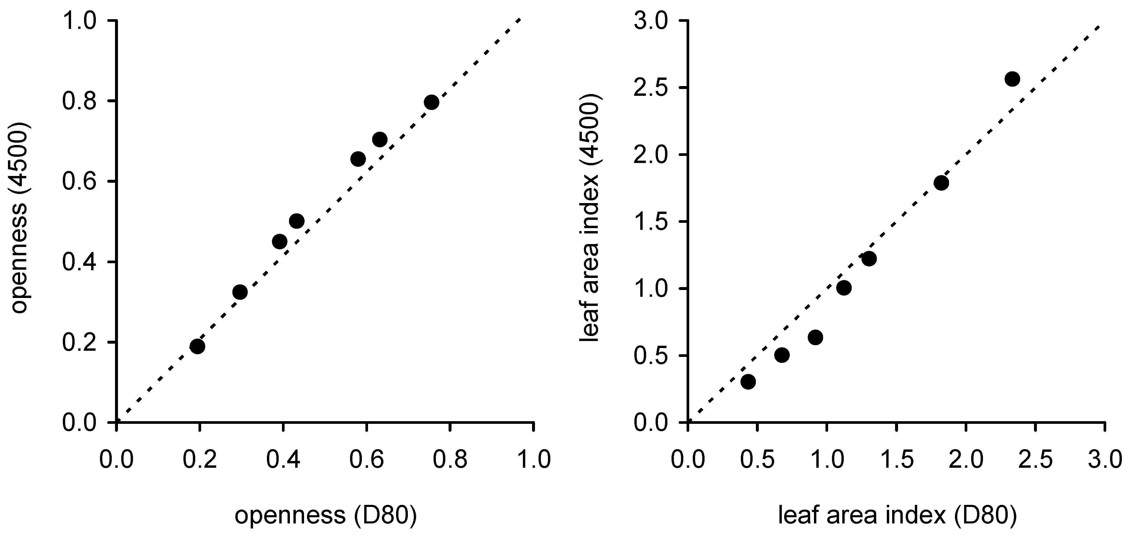
not suggest a minimum pixel number above which canopy analyses are independent of image size: both the Coolpix 900 and Coolpix 990 had the same minimum image size (640 × 480) but the Coolpix 990 had a larger maximum image size, so it would have been expected that variation in canopy traits would be greatest in the 990 owing to its larger range of image sizes. Instead, the results of the current and previous studies lead us to conclude that canopy analyses are largely independent of image size in newer cameras either as a result of better quality lenses or sensors.
The choice of camera did affect the results from both fisheye photography and DCP. While the 4500 produced larger estimates of openness from fisheye photographs, it produced smaller estimates of crown porosity from cover photographs compared to the D80. The differences between cameras were large enough to result in different estimates of
LAI from fisheye photography but not DCP, except for one site (
Figure 4). The site at which
LAI estimates from DCP were different was the site with the tallest trees and largest cover; hence, we speculate that the performance of the two cameras may differ more in taller, denser canopies. The larger mean leaf inclination angle and openness indicate that the canopy analysis was detecting larger gaps near the centre of the 4500 fisheye images than the D80 images. This might be accounted for by differences in photographic exposure despite every care being taken to make these as similar as possible, but may also indicate more vignetting in the FC-E8 fisheye converter compared to the 10.5mm fisheye lens, which can result in over-exposure at the zenith. In contrast, the smaller crown porosity measured using the 4500 suggests more mixed pixels in images from this camera than from the D80. Frazer
et al. [
27] noted that there was more blurring in images from the Coolpix 950 than in images from a 35 mm film SLR camera. It is likely that the D80 together with fixed angle lenses produces sharper images with better contrast and more even illuminance than the 4500 with its built in zoom lens, either with or without a fisheye converter. It is worth noting that estimates of foliage or crown cover and
LAI from the two cameras generally varied by less than 15%, and that this is similar to the uncertainty associated with direct estimates of
LAI from tree harvesting [
9]; past estimates of leaf area or foliage and crown cover from the Coolpix range of cameras are by no means invalid, and inexpensive cameras (e.g., point-and-shoot) can obtain good results from DCP provided that the field-of-view (FOV) can be controlled. However, FOV is more easily controlled with fixed angle lenses on DSLR cameras, which also have superior optics, better battery life, lower-noise sensors and greater ISO range.
Changing the ISO equivalence of the D80 and 4500 had a statistically detectable effect on foliage cover and crown cover as well as crown porosity from cover images, but the effect was so small that it would not be an important obstacle to using higher ISO equivalence to simultaneously achieve both faster shutter speeds and smaller apertures (thus increasing depth of field) for image capture in dark or windy conditions. Previous tests of the D80 concluded that increasing ISO does not greatly increase signal noise up to ISO 800 but that there is significant noise at ISO 1,600 [
30,
45]. However, we found that estimates of canopy variables from DCP were so little affected by this that we can see no obstacle to using the D80 routinely at ISO 200 or ISO 400 for canopy photography and that ISO 800 or even ISO 1600 could be used in conditions of low light and moderate wind. Even the highest ISO equivalence on the 4500 had little impact on estimates of foliage cover and crown cover or porosity. Our comparison included canopies with a wide range of structures, including some needle-leaved species, and our findings should we widely applicable but, of course, we recommend that users test their own equipment in their own situation. Given the small effect of ISO equivalence on measurements of canopy structure we conclude that differing signal-to-noise ratios of the CCDs in the two cameras is not the main cause of the different results from the two cameras.
Increasing the threshold luminance value increased cover and
LAI as expected; the proportions of pixels classified as sky or foliage will change as the threshold value changes. Crown porosity also generally decreases as the threshold is increased owing to the shrinking size of the gaps within crowns as the overall area of cover increases—more pixels on the edge of gaps are also classified as foliage rather than sky. However, the trend was less clear for porosity; porosity sometimes increased despite a smaller threshold value and sometimes decreased despite a larger threshold. This is probably the result of foliage and branches near the edge of crowns joining together (in the image) as the classified image darkened causing new within-crown gaps to form near the canopy edge. Overall, the small impact of even large changes to the threshold value on estimates of cover and
LAI reflects the small proportion of mixed pixels in high-resolution cover images and illustrates the robustness of the DCP method. Fuentes
et al. [
17] also observed little impact of threshold variations on estimated
LAI from DCP.
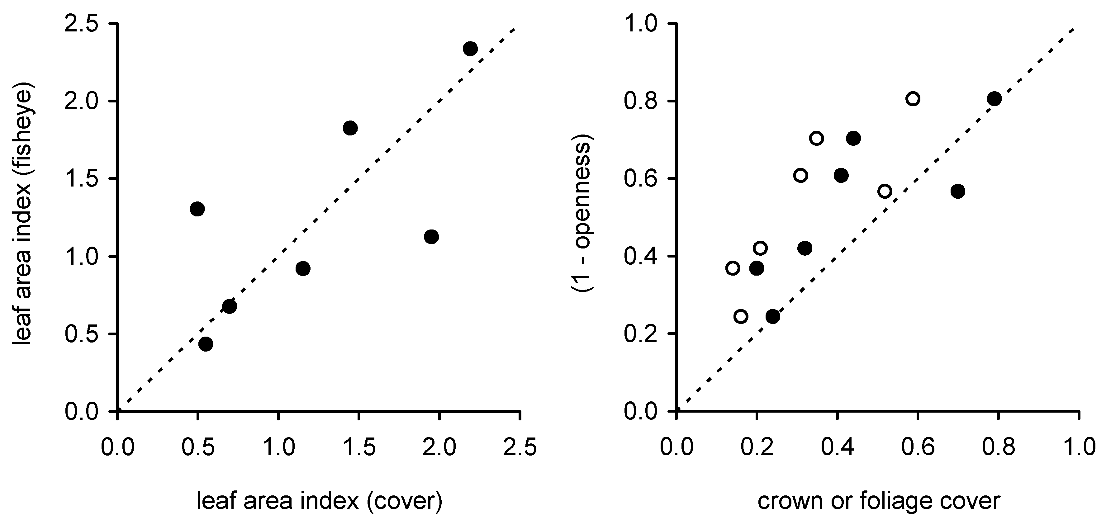
LAI from fisheye photography agreed best with that from DCP (our reference method owing to its previous calibration in this forest type) when the crown cover from cover images was similar to 1-openness from fisheye images (
Figure 7). There is no
a priori reason to expect that openness and crown cover should be directly related: openness was averaged over a zenith angle range from 0° to 70° while crown cover is the vertical projection of
solid crowns. We believe that the close agreement between openness and crown cover (for sites where estimated
LAI was similar) derives from 1) the wider zenith range sampled by the fisheye method resulting in a larger estimate of cover compared to DCP; crown and foliage cover naturally increase with increasing zenith angle, and 2) the fact that fisheye photography does not detect very small gaps, resulting in probable underestimation of the true openness and measurement of a quantity that is analogous to something between crown cover and foliage cover. This comparison of openness and cover suggests the number of fisheye images collected at each plot in this study may have been insufficient and biased either towards large gaps or dense cover at the three sites where the two photographic methods yielded contrasting estimates of
LAI. An apparent advantage of fisheye photography over DCP and other single zenith angle methods is that fisheye sensors integrate over a wide area and fewer images are needed. However, it is likely that the number of samples collected, even using fisheye sensors, must be larger than that used in this study to obtain accurate estimates of
LAI. Differences between the two methods make a direct comparison of data other than
LAI difficult. For example, although both methods measure the gap fraction near the zenith, fisheye photography does so with less accuracy owing to its poorer spatial resolution, the smaller number of images collected (which results in greater variability near the zenith [
46,
47]) and over-exposure or blooming near the zenith as a result of poor exposure, lens vignetting or sky luminance variations [
48,
49,
50]; hence, a comparison of vertical cover between the two methods is necessarily disadvantageous to fisheye photography. We also note that estimates of vertical cover obtained from fisheye methods should be treated with caution.
The greater accuracy with which DCP measures vertical cover makes it particularly suited to calibrating and testing remotely sensed forest metrics obtained from high-resolution airborne LIDAR and aerial stereo photography [
51,
52] that often have a very vertical FOV similar to that of DCP but very unlike the wide angle of fisheye sensors. This has not been exploited to date: published studies have used DCP to calibrate coarse-scale spectral imagery from Landsat [
16] and MODIS [
17] against plot-scale
LAI. Correlation coefficients of 0.8–0.9 between remotely sensed spectral indices and
LAI measured using DCP were reported. Boer
et al. [
16] were able to map both the extent and severity of wildfire based on reduction in
LAI, and Fuentes
et al. [
16] showed that the
LAI from MODIS agreed with
LAI estimated from DCP to within 0.3 units. These good correlations were obtained despite upward-looking methods such as DCP and ground-based fisheye sensors not sampling understorey, whereas downward-looking remote sensing technologies will sample understorey, especially when based on spectral indices. Understorey contributed little to the overall spectral signal from Landsat in jarrah forest [
16] but this may not always be the case. Understorey cover may also be estimated from downward-looking ground-based photography using methods analogous to those described in this manuscript [
53].
While these studies already demonstrate the utility of DCP, we believe that the method will ultimately be even more useful for calibrating and testing metrics obtained from finer-scale remote sensing methods and analyses that utilize morphological processing rather than relying solely on spectral indices [
54,
55]. For example, vertical FOV remote sensing methods can potentially provide estimates of crown cover that can be compared directly with those obtained from DCP. This is especially the case for remote sensing technologies that use height data extracted from three-dimensional interpretations of stereo imagery or LIDAR waveforms to more accurately define the boundary of tree crowns [
54,
55]. Crown cover has the advantage of not requiring knowledge of the foliage inclination angle distribution and is measured with great accuracy using DCP; hence, crown cover is a very good starting place for ground-truthing metrics derived from morphological analyses of remotely sensed data. For monitoring gross changes in vegetation extent, crown cover may be suitable and conversion to
LAI not required. However, vertical FOV remote sensing methods can potentially also provide estimates of individual tree crown areas that could be used as predictors for tree biomass. Chave
et al. [
56] obtain good correlations between tree diameter and above-ground biomass and carbon in tropical forest across a range of species and concluded that they were able to accurately estimate above-ground carbon in a wide range of forests based on their models; however, tree diameter data are not readily available over large areas. Crown area can also be used an independent variable in allometric relationships (see [
57] for example) and could be estimated from vertical FOV remote sensing methods. DCP is the ideal ground-based method for plot-scale calibration and testing of remote sensing methods aimed at this application.
While studies to date have concentrated on plot-scale calibrations of remotely sensed metrics, DCP could also be used to provide very accurate gap fraction information at more local scales (a few square meters) either along transects or directly beneath canopies. Ground-based measurements of crown porosity could be used to calibrate remotely sensed spectral information from within crowns following crown delineation using morphological image analysis methods. In very sparse vegetation DCP could be combined with more traditional line and point intercept methods [
58] for estimating crown cover; for example, crown cover in plots or along transects could be rapidly estimated from visual presence/absence of crowns while crown porosity is obtained from fewer DCP images taken directly beneath crowns, thus eliminating the need for collecting many empty photographic images.
Although DCP was originally devised for sparse to moderately dense broadleaf forest, DCP has also recently been tested in very sparse savanna woodland [
36]; DCP was superior to four other methods tested for estimating crown cover and
LAI in that study and, used in combination with the Licor
LAI-2000, was also able to quantify the element clumping index in this highly clumped vegetation type. We believe that DCP will also be well suited to very dense forest, in which its ability to detect small gaps in crowns would result in more accurate gap fraction retrieval (near the zenith) than is possible with fisheye sensors. For example, in relation to boreal forests and gap fraction inversion methods, Nilson [
32] noted that “For canopies with nearly nontransparent crowns the result of inversion is rather an estimate of the crown surface area index” and that “The amount of gaps within tree crowns is the main source of information in the estimation of crown density”. Given the much higher spatial resolution of DCP compared to fisheye methods there can be little doubt that it would provide a better estimate of the gap fraction within crowns, albeit at a single zenith angle. In addition to the accuracy of gap fraction retrieval, the applicability of DCP to variable-density forest makes it ideally suited to measurement of cover and
LAI in research and monitoring plots, as well as in transects.


