Regional Assessment of Aspen Change and Spatial Variability on Decadal Time Scales

Abstract
:1. Introduction
2. Methods
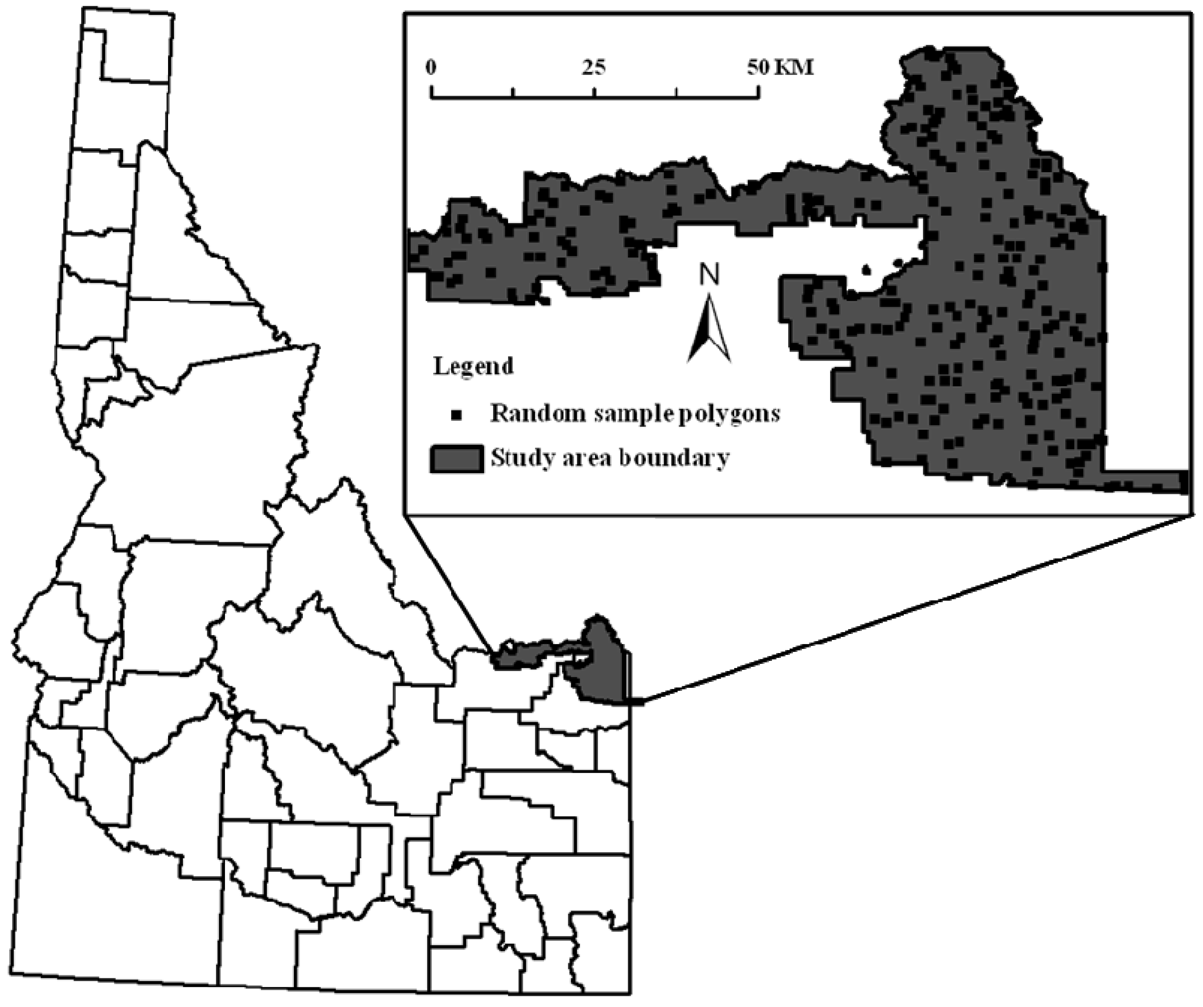
2.1. Study Site

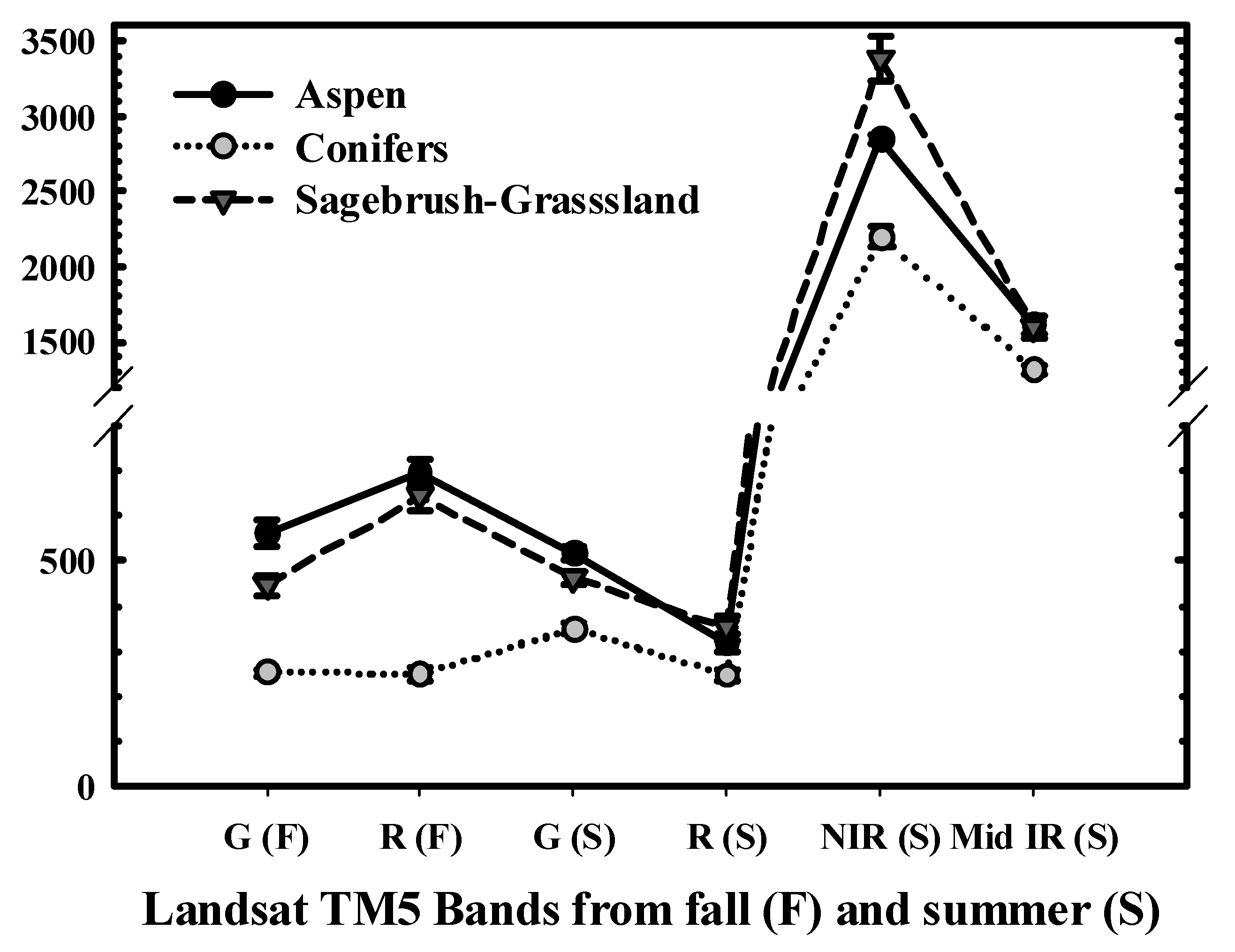
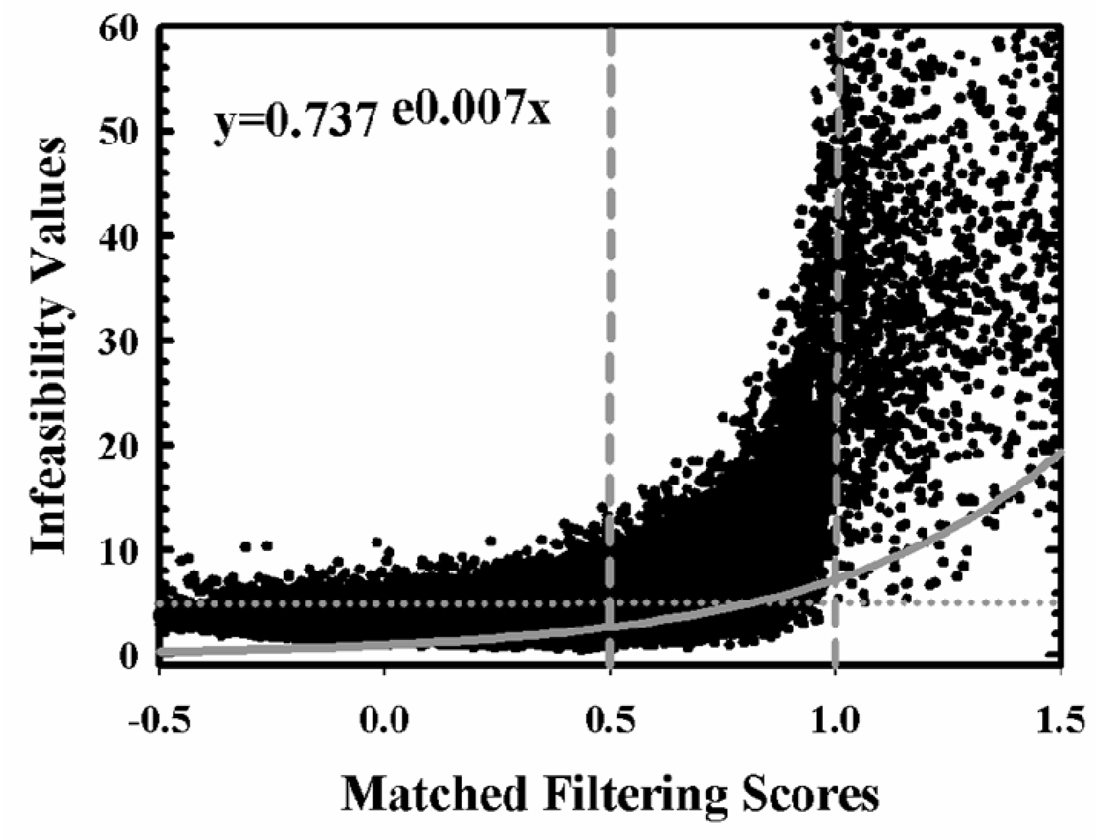
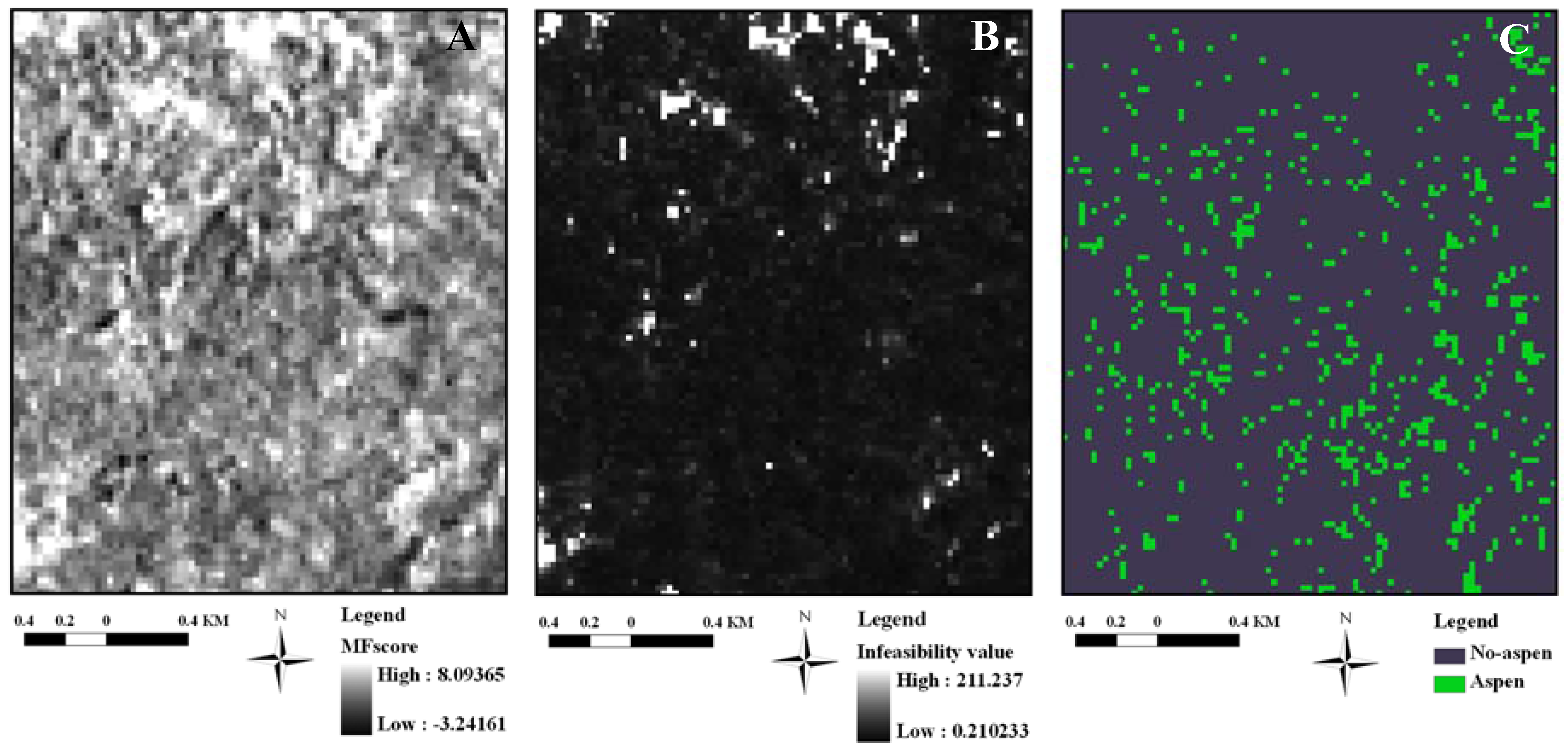
2.2. Aspen Maps and Image Classification


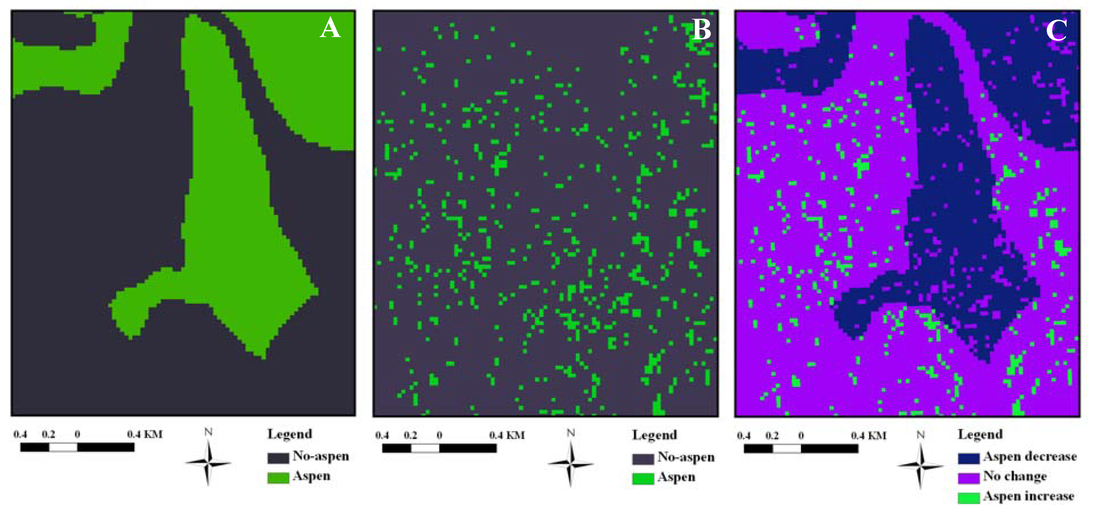
2.3. Aspen Change Detection

2.4. GIS-Derived Variables
2.5. Statistical Analysis
3. Results
3.1. Aspen Maps and Image Classification

| Observed/Classified | Aspen | No-aspen | Row Total |
|---|---|---|---|
| Aspen | 73 | 13 | 86 |
| No-aspen | 15 | 274 | 289 |
| Column total | 88 | 287 | |
| Producer’s accuracy | 83% | 95% | |
| User’s accuracy | 85% | 95% | |
| Overall accuracy | 93% |
| Observed/Classified | Aspen | No-aspen | Row Total |
|---|---|---|---|
| Aspen | 80 | 20 | 100 |
| No-aspen | 12 | 263 | 275 |
| Column total | 92 | 283 | |
| Producer’s accuracy | 87% | 93% | |
| User’s accuracy | 80% | 96% | |
| Overall accuracy | 92% |
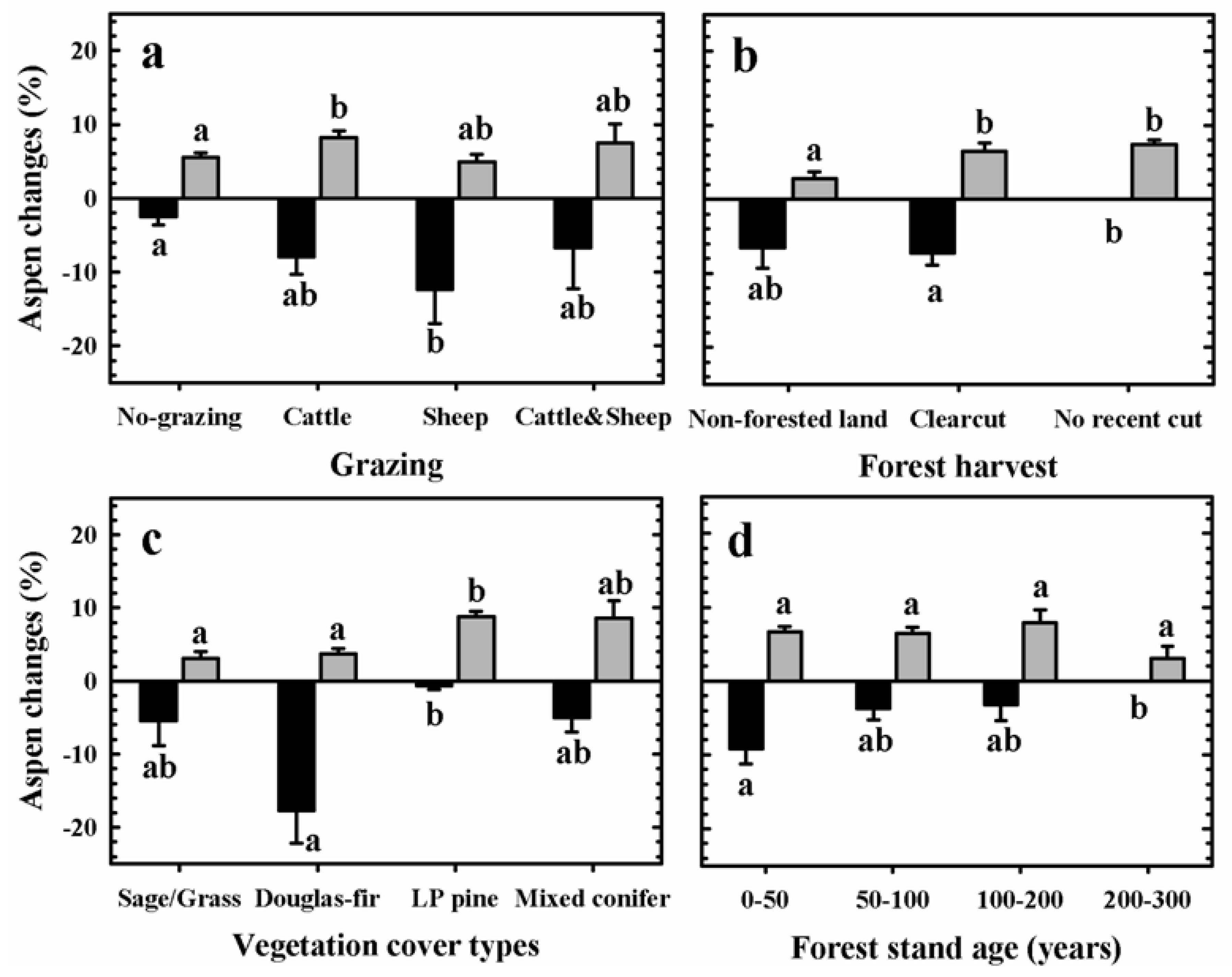
3.2. Aspen Change: 1920–2005

| Predictor variables | Aspen change patterns | MANOVA test p-values |
|---|---|---|
| 1920–2005 period | ||
| Grazing | Increase Decrease | 0.002 < 0.001 |
| Forest harvest | Increase Decrease | < 0.001 0.011 |
| Stand age | Increase Decrease | 0.081 0.05 |
| Vegetation cover | Increase Decrease | 0.001 0.019 |
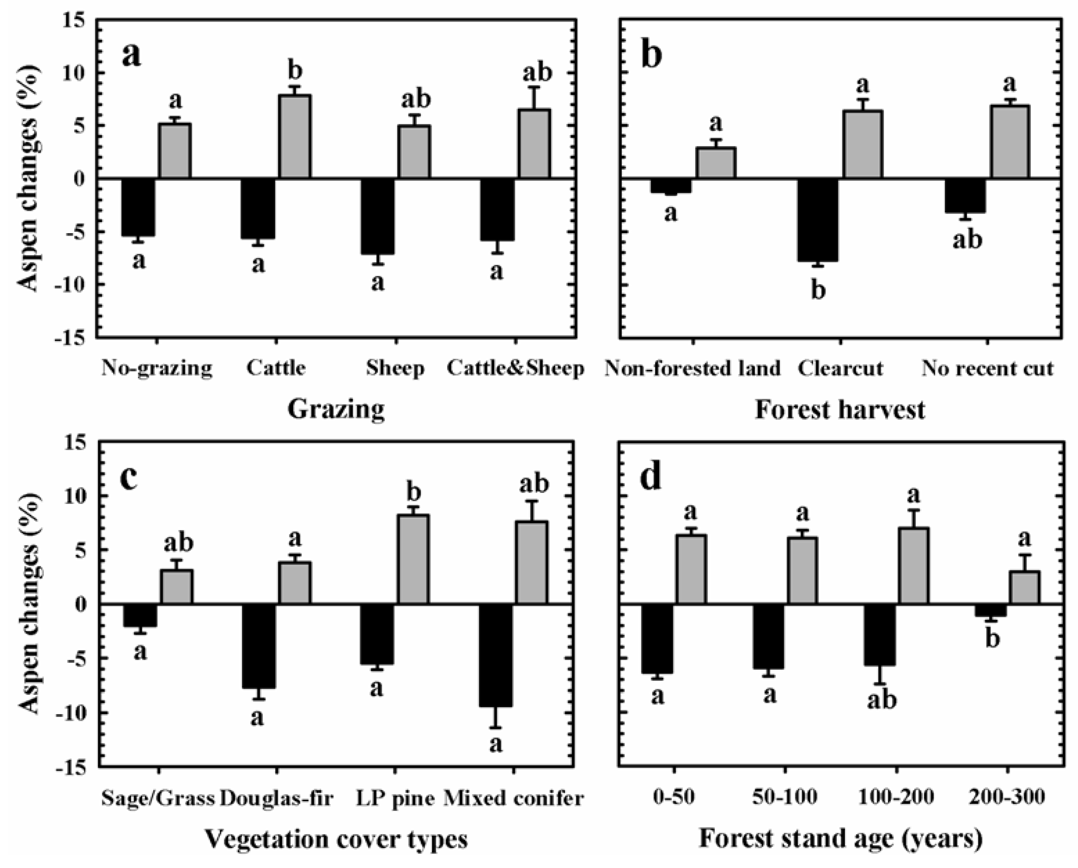
| 1987–2005 period | ||
| Grazing | Increase Decrease | 0.152 0.006 |
| Forest harvest | Increase Decrease | < 0.001 0.216 |
| Stand age | Increase Decrease | 0.187 0.05 |
| Vegetation cover | Increase Decrease | < 0.001 0.674 |
3.3. Aspen Change: 1987–2005

4. Discussion
4.1. Aspen Classification
4.2. Aspen Change Detection
5. Conclusions
Acknowledgements
References and Notes
- Bartos, D.L.; Mueggler, W.F. Early succession in aspen communities following fire in Western Wyoming. J. Range Manage. 1981, 34, 315–318. [Google Scholar] [CrossRef]
- Bartos, D.L. Landscape dynamics of aspen and conifer forests. In Sustaining Aspen in Western Landscapes: Symposium Proceedings, Grand Junction, CO, USA, June 13–15, 2000; USDA Forest Service, Rocky Mountain Research Station: Fort Collins, CO, USA, RMRS-P-18, 2001; pp. 5–14. [Google Scholar]
- Kilpatrick, S.; Abendroth, D. Aspen response to prescribed fire and wild ungulate herbivory. In Sustaining Aspen in Western Landscapes: Symposium Proceesings, Grand Junction, CO, USA, June 13–15, 2000; USDA Forest Service, Rocky Mountain Research Station: Fort Collins, CO, USA RMRS-P-18. , 2001. [Google Scholar]
- Zier, J.L.; Baker, W.L. A century of vegetation change in the San Juan Mountains, Colorado: an analysis using repeat photography. For. Ecol. Manage. 2006, 228, 251–262. [Google Scholar] [CrossRef]
- Sankey, T.T. Learning from spatial variability: Aspen persistence in the Centennial Valley, Montana. For. Ecol. Manage. 2008, 255, 1219–1225. [Google Scholar] [CrossRef]
- Barnett, D.T.; Stohlgren, T.J. Aspen persistence near the National Elk Refuge and Gros Ventre Valley elk feedgrounds of Wyoming, USA. Lands. Ecol. 2001, 16, 569–580. [Google Scholar] [CrossRef]
- Manier, D.J.; Laven, R.D. Changes in landscape patterns associated with the persistence of aspen (Populus tremuloides Michx.) on the western slope of the Rocky Mountains, Colorado. For. Ecol. Manage. 2002, 167, 263–284. [Google Scholar] [CrossRef]
- Kaye, M.W.; Stohlgren, T.J.; Binkley, D. Aspen structure and variability in Rocky Mountain National Park, Colorado, USA. Lands. Ecol. 2003, 18, 591–603. [Google Scholar] [CrossRef]
- Brown, K.; Hansen, A.J.; Keane, R.E.; Graumlich, L.J. Complex interactions shaping aspen dynamics in the Greater Yellowstone Ecosystem. Lands. Ecol. 2006, 21, 933–951. [Google Scholar] [CrossRef]
- DeByle, N.V.; Winokur, R.P. Aspen: Ecology and Management in the Western United States; General Technical Report RM-119; Rocky Mountain Forest and Research Station: Fort Collins, CO, USA, 1985. [Google Scholar]
- Turner, M.G.; Romme, W.H.; Reed, R.A.; Tuskan, G.A. Post-fire aspen seedling recruitment across the Yellowstone (USA) Landscape. Lands. Ecol. 2003, 18, 127–140. [Google Scholar] [CrossRef]
- Romme, W.H.; Turner, M.G.; Tuskan, G.A.; Reed, R.A. Establishment, persistence, and growth of aspen (Populus tremuloides) seedlings in Yellowstone National Park. Ecology 2005, 86, 404–418. [Google Scholar] [CrossRef]
- Romme, W.H.; Turner, M.G.; Wallace, L.L.; Walker, J.S. Aspen, elk, and fire in northern Yellowstone Park. Ecology 1995, 76, 2097–2106. [Google Scholar] [CrossRef]
- Kay, E.C.; Bartos, D.L. Ungulate herbivory on Utah aspen: Assessment of long-term exclosures. J. Range Manage. 2000, 53, 145–153. [Google Scholar] [CrossRef]
- Ripple, W.J.; Larsen, E.J. Historic aspen recruitment, elk, and wolves in northern Yellowstone National Park, USA. Biol. Cons. 2000, 95, 361–370. [Google Scholar] [CrossRef]
- Hessl, A.E.; Graumlich, L.J. Interactive effects of human activities, herbivory, and fire on quaking aspen (Populus tremuloides) age structures in western Wyoming. J. Biog. 2002, 29, 889–902. [Google Scholar] [CrossRef]
- Fitzgerald, R.D.; Bailey, A.W. Control of aspen regrowth by grazing with cattle. J. Range Manage. 1984, 37, 156–158. [Google Scholar] [CrossRef]
- Bailey, A.W.; Irving, B.D.; Fitzgerald, R.D. Regeneration of woody species following burning and grazing in Aspen Parkland. J. Range Manage. 1990, 43, 212–215. [Google Scholar] [CrossRef]
- Rumble, M.A.; Pella, T.; Sharps, J.C.; Carter, A.V.; Parrish, B. Effects of logging slash on aspen regeneration in grazed clear-cuts. Prairie Nat. 1996, 28, 199–210. [Google Scholar]
- Kimble, D.S. Quaking aspen (Populus tremuloides) ecology on Forest Service lands north of Yellowstone National Park. Master Thesis, Montana State University, Bozeman, MT, USA, 2007. [Google Scholar]
- Weatherill, R.G.; Keith, L.B. The Effect of Livestock Grazing on an Aspen Forest Community; Technical Bulletin 1; Department of Lands and Forests, Fish and Wildlife Division: Ottawa, CA, 1969; Volume 1. [Google Scholar]
- Smith, A.D.; Lucas, P.L.; Baker, C.O.; Scotter, G.W. The Effects of Deer and Domestic Livestock on Aspen Regeneration in Utah; Utah Division of Wildlife Resources: Salt Lake City, UT, USA, 1972; No. 72–1. [Google Scholar]
- Mallik, A.U.; Bell, F.W.; Gong, Y. Regeneration behavior of competing plants after clear cutting: implications for vegetation management. For. Ecol. Manage. 1997, 95, 1–10. [Google Scholar] [CrossRef]
- Newsome, T.; Heineman, J.; Linnell Nemec, A. Competitive interactions between juvenile trembling aspen and lodgepole pine: a comparison of two interior British Columbia ecosystems. For. Ecol. Manage. 2008, 255, 2950–2962. [Google Scholar] [CrossRef]
- Mueggler, M. Age distribution and reproduction of intermountain aspen stands. West. J. Appl. For. 1989, 4, 41–45. [Google Scholar]
- Wolter, P.T.; Mladenoff, D.J.; Host, G.E.; Crow, T.R. Improved forest classification in the northern lake states using multi-temporal Landsat imagery. Photo. Eng. Rem. Sens. 1995, 61, 1129–1143. [Google Scholar]
- Arsenault, E.J.; Hall, R.J.; Skakun, R.S.; Hogg, E.H.; Michaelian, M. Characterizing aspen dieback severity using multidate Landsat data in western Canadian forests. In Eleventh Forest Service Remote Sensing Applications Conference, Salt Lake City, UT, USA, April 24–28, 2006.
- Bork, E.W.; Su, J.G. Integrating LIDAR data and multispectral imagery for enhanced classification of rangeland vegetation: a meta analysis. Rem. Sens. Env. 2007, 111, 11–24. [Google Scholar] [CrossRef]
- McRoberts, R.E. Using satellite imagery and the k-nearest neighbors technique as a bridge between strategies and management forest inventories. Rem. Sens. Env. 2008, 112, 2212–2221. [Google Scholar] [CrossRef]
- Lillesand, T.M.; Kiefer, R.W. Remote Sensing and Image Interpretation, 4th ed.; John Wiley & Sons: New York, NY, USA, 2000; p. 568. [Google Scholar]
- Adams, J.B.; Smith, M.O.; Johnson, P.E. Spectral mixture modeling: a new analysis of rock and soil types at the Viking Lander 1 site. J. Geophys. Res. 1986, 91, 8098–8112. [Google Scholar] [CrossRef]
- Small, C. The Landsat ETM+ spectral mixing space. Rem. Sens. Env. 2004, 93, 1–17. [Google Scholar]
- Xiao, J.; Moody, A. A comparison of methods for estimating fractional green vegetation cover within a desert-to-upland transition zone in central New Mexico, USA. Rem. Sens. Env. 2005, 98, 237–250. [Google Scholar] [CrossRef]
- Rencz, A.N. Remote Sensing for the Earth Sciences; John Wiley & Sons: New York, NY, USA, 1999; pp. 251–307. [Google Scholar]
- Chen, X.; Vierling, L.; Rowell, E.; DeFelice, T. Using lidar and effective LAI data to evaluate IKONOS and Landsat 7 ETM+ vegetation cover estimates in a ponderosa pine forest. Rem. Sens. Env. 2004, 91, 14–26. [Google Scholar] [CrossRef]
- Small, C.; Lu, J.W.T. Estimation and vicarious validation of urban vegetation abundance by spectral mixture analysis. Rem. Sens. Env. 2006, 100, 441–456. [Google Scholar] [CrossRef]
- Sankey, T.T.; Germino, M.J. Assessment of juniper encroachment with the use of satellite imagery and geospatial data. Range. Ecol. Manage. 2008, 61, 412–418. [Google Scholar] [CrossRef]
- USDA Natural Resources Conservation Service. Soil survey. Available online: http://websoilsurvey.nrcs.usda.gov/app/ ( accessed on April 2, 2009).
- The Targhee National Forest. Revised Forest Plan. Final Environmental Impact Statement. Chapter III: Affected Environment; The Targhee National Forest: Idaho Falls, ID, USA, 1997; pp. 1–7. [Google Scholar]
- Bergen, K.; Dronova, I. Observing succession on aspen-dominated landscapes using a remote sensing-ecosystem approach. Lands. Ecol. 2007, 22, 1395–1410. [Google Scholar] [CrossRef]
- Boardman, J.W. Leveraging the high dimensionality of AVIRIS data for improved sub-pixel target unmixing and rejection of false positives: Mixture tuned matched filtering. In AVIRIS 1998 Proceedings; JPL: Pasadena, CA, USA, 1998; p. 6. [Google Scholar]
- Mitchell, J.; Glenn, N. Leafy spurge (Euphorbia esula L.) classification performance using hyperspectral and multispectral sensors. Range. Ecol. Manage. 2009, 62, 16–27. [Google Scholar] [CrossRef]
- Kulakowski, D.; Veblen, T.T.; Drinkwater, S. The persistence of quaking aspen (Populus tremuloides) in the Grand Mesa area, Colorado. Ecol. Appl. 2004, 14, 1601–1614. [Google Scholar] [CrossRef]
- Kulakowski, D.; Veblen, T.T.; Kurzel, B.P. Influences of infrequent fire, elevation, and pre-fire vegetation on the persistence of quaking aspen (Populus tremuloides Michx) in the Flat Tops area, Colorado, USA. J. Biog. 2006, 33, 1397–1413. [Google Scholar] [CrossRef]
- Baker, W.L.; Munroe, J.A.; Hessl, A.E. The effects of elk on aspen in the winter range in Rocky Mountain National Park. Ecography 1997, 20, 155–165. [Google Scholar] [CrossRef]
- Di Orio, A.P.; Callas, R.; Schaefer, R.J. Forty-eight year decline and fragmentation of aspen (Populus tremuloides) in the South Warner Mountain of California. For. Ecol. Manage. 2005, 206, 307–313. [Google Scholar] [CrossRef]
- Gallant, A.L.; Hansen, A.J.; Councilman, J.S.; Monte, D.K.; Betz, D.W. Vegetation dynamics under fire exclusion and logging in a Rocky Mountain watershed, 1856–1996. Ecol. Appl. 2003, 13, 385–403. [Google Scholar] [CrossRef]
- Kurzel, B.P.; Veblen, T.T.; Kulakowski, D. A typology of stand structure and dynamics of quaking aspen in northwestern Colorado. For. Ecol. Manage. 2007, 252, 176–190. [Google Scholar] [CrossRef]
- Suzuki, K.; Suzuki, H.; Binkley, D.; Stohlgren, T.J. Aspen regeneration in the Colorado Front Range: differences at local and landscape scales. Lands. Ecol. 1999, 14, 231–237. [Google Scholar] [CrossRef]
© 2009 by the authors; licensee Molecular Diversity Preservation International, Basel, Switzerland. This article is an open-access article distributed under the terms and conditions of the Creative Commons Attribution license (http://creativecommons.org/licenses/by/3.0/).
Share and Cite
Sankey, T.T. Regional Assessment of Aspen Change and Spatial Variability on Decadal Time Scales. Remote Sens. 2009, 1, 896-914. https://doi.org/10.3390/rs1040896
Sankey TT. Regional Assessment of Aspen Change and Spatial Variability on Decadal Time Scales. Remote Sensing. 2009; 1(4):896-914. https://doi.org/10.3390/rs1040896
Chicago/Turabian StyleSankey, Temuulen Tsagaan. 2009. "Regional Assessment of Aspen Change and Spatial Variability on Decadal Time Scales" Remote Sensing 1, no. 4: 896-914. https://doi.org/10.3390/rs1040896