An Improved ASTER Index for Remote Sensing of Crop Residue


 and
and
Abstract
:
1. Introduction

2. Remote Sensing Crop Residue Cover
2.1. Spectral Properties of Soils and Residues
2.2. Previously Existing Spectral Indices for Crop Residue Detection


| Location | Beltsville, MD | CMD | Ames, IA | Fulton, IN | PIL | Composite (mean) value | ||||||||
| Date | 20 May 2002 | 22 May 2002 | 10 Jun 2003 | 1 Jun 2004 | 2 Jun 2004 | 10 Apr 2007 | 22 May 2005 | 19 May 2007 | 27 May 2007 | 29 May 2006 | 6 Jun 2007 | 8 Jun 2006 | ||
| Sensor | Ground | Air-borne | ASTER | Air-borne | Airborne | Air-borne | ||||||||
| N | 77 | 95 | 41 | 41 | 71 | 32 | 107 | 104 | 104 | 95 | 136 | 37 | ||
| Residue Water g g–1 | 0.09 | 0.08 | 1.80 | 1.10 | 0.10 | dna | dna | dna | dna | dna | dna | dna | ||
| Soil Water g g–1 | dna | 0.09 | 0.30 | 0.28 | 0.09 | dna | dna | dna | dna | dna | dna | dna | ||
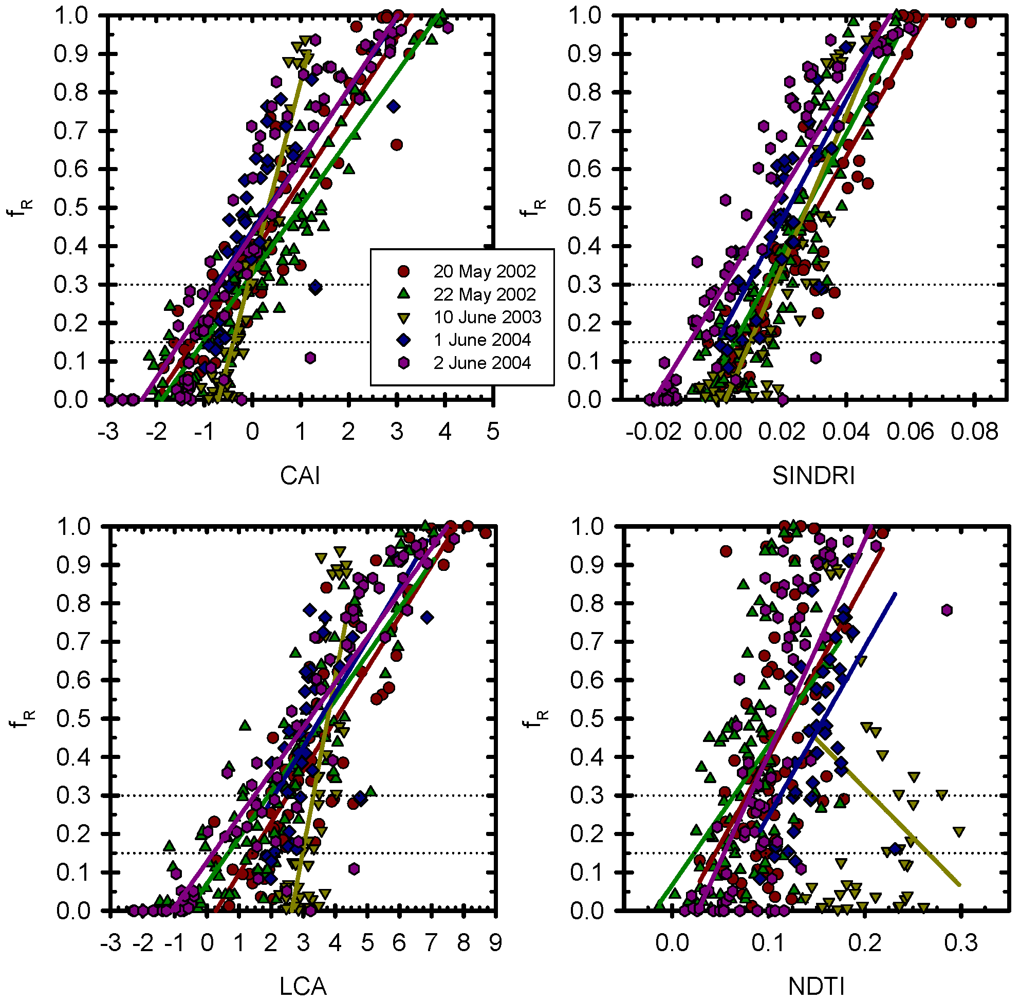
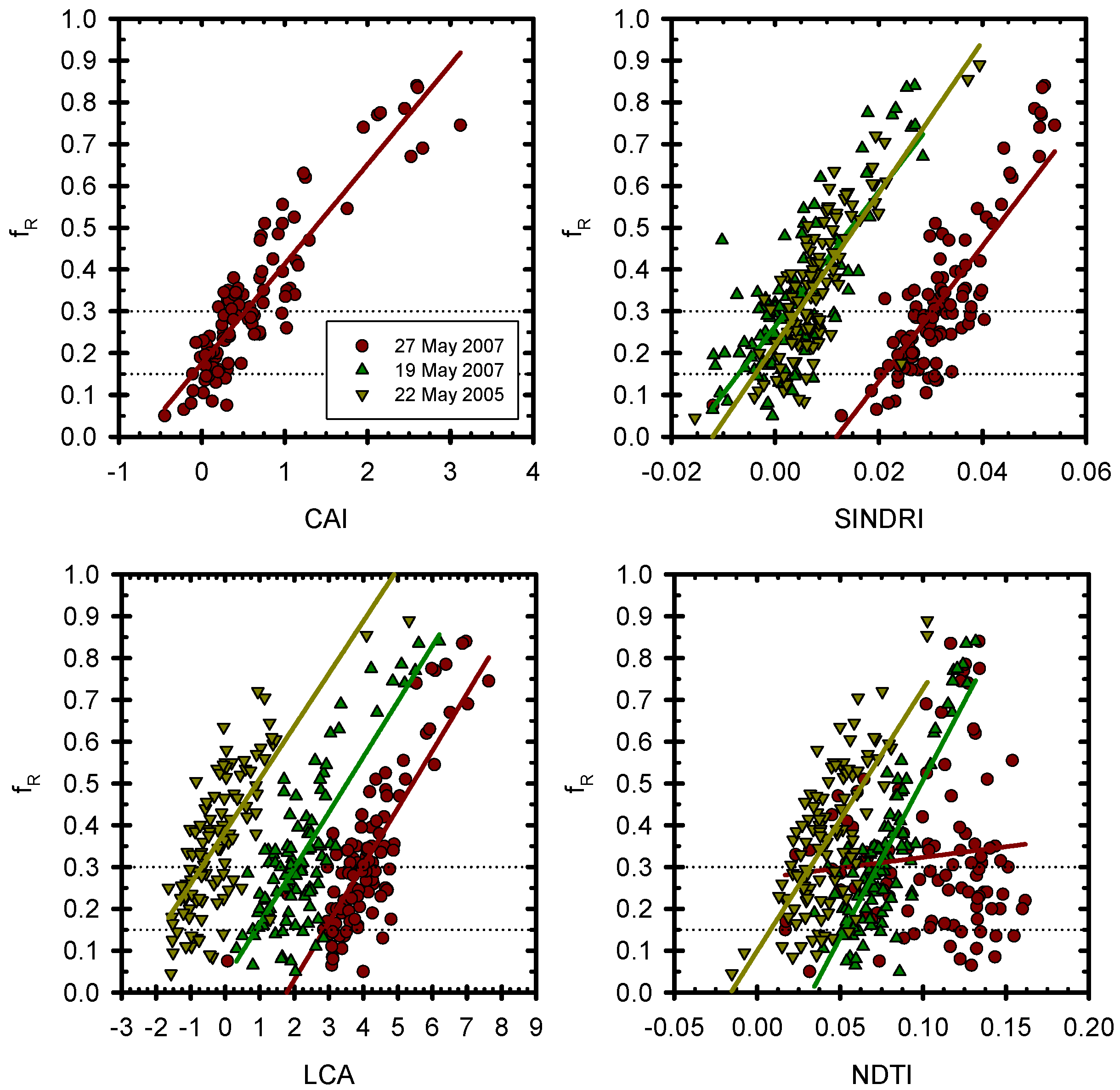
| CAI | r2 | 0.899 | 0.882 | 0.935 | 0.554 | 0.815 | 0.885 | bna | bna | 0.821 | 0.798 | 0.829 | 0.722 | 0.814 |
| RMSE | 0.097 | 0.094 | 0.085 | 0.151 | 0.152 | 0.100 | bna | bna | 0.078 | 0.117 | 0.107 | 0.128 | 0.111 | |
| 3×3 acc. | 0.829 | 0.779 | 0.902 | 0.732 | 0.761 | 0.813 | bna | bna | 0.654 | 0.674 | 0.695 | 0.757 | 0.759 | |
| k-hat | 0.68 | 0.63 | 0.84 | 0.13 | 0.61 | 0.66 | bna | bna | 0.42 | 0.51 | 0.45 | 0.51 | 0.54 | |
| Z-stat | 8.90 | 9.62 | 11.82 | 0.77 | 8.19 | 5.81 | bna | bna | 5.26 | 6.73 | 5.43 | 3.62 | 6.61 | |
| SINDRI | r2 | 0.853 | 0.811 | 0.769 | 0.640 | 0.835 | 0.596 | 0.611 | 0.605 | 0.674 | 0.821 | 0.834 | 0.868 | 0.743 |
| RMSE | 0.117 | 0.119 | 0.159 | 0.135 | 0.144 | 0.187 | 0.106 | 0.116 | 0.106 | 0.093 | 0.106 | 0.088 | 0.123 | |
| 3 × 3 acc. | 0.855 | 0.768 | 0.805 | 0.780 | 0.887 | 0.750 | 0.710 | 0.587 | 0.712 | 0.653 | 0.811 | 0.784 | 0.758 | |
| k-hat | 0.73 | 0.61 | 0.69 | 0.43 | 0.81 | 0.53 | 0.42 | 0.30 | 0.51 | 0.48 | 0.68 | 0.57 | 0.56 | |
| Z-stat | 9.93 | 9.19 | 7.48 | 3.22 | 12.96 | 4.13 | 5.56 | 3.95 | 6.93 | 6.39 | 10.16 | 4.21 | 7.01 | |
| LCA | r2 | 0.815 | 0.767 | 0.634 | 0.487 | 0.842 | 0.651 | 0.575 | 0.632 | 0.664 | 0.390 | 0.618 | 0.860 | 0.661 |
| RMSE | 0.131 | 0.132 | 0.200 | 0.161 | 0.140 | 0.174 | 0.111 | 0.112 | 0.107 | 0.171 | 0.161 | 0.091 | 0.141 | |
| 3 × 3 acc. | 0.737 | 0.737 | 0.780 | 0.707 | 0.789 | 0.813 | 0.673 | 0.606 | 0.587 | 0.547 | 0.611 | 0.703 | 0.691 | |
| k-hat | 0.51 | 0.55 | 0.64 | 0.09 | 0.63 | 0.66 | 0.34 | 0.33 | 0.29 | 0.34 | 0.34 | 0.43 | 0.43 | |
| Z-stat | 6.18 | 7.87 | 6.61 | 0.57 | 7.71 | 5.51 | 4.04 | 4.11 | 3.67 | 4.17 | 4.22 | 2.97 | 4.80 | |
| NDTI | r2 | 0.281 | 0.247 | 0.089 | 0.272 | 0.569 | 0.229 | 0.490* | 0.640* | 0.004 | 0.419 | 0.182 | 0.161 | 0.299 |
| RMSE | 0.258 | 0.227 | 0.316 | 0.192 | 0.232 | 0.259 | 0.122* | 0.111* | 0.185 | 0.167 | 0.235 | 0.222 | 0.210 | |
| 3 × 3 acc. | 0.618 | 0.589 | 0.366 | 0.780 | 0.634 | 0.563 | 0.720* | 0.625* | 0.462 | 0.463 | 0.589 | 0.649 | 0.588 | |
| k-hat | 0.16 | 0.28 | 0.11 | 0.32 | 0.37 | 0.12 | 0.44* | 0.37* | 0.01 | 0.22 | 0.24 | 0.33 | 0.25 | |
| Z-stat | 1.49 | 3.48 | 0.73 | 1.92 | 4.07 | 0.76 | 5.28* | 4.94* | 0.06 | 2.61 | 2.48 | 1.80 | 2.47 | |
3. Spectral Data Acquisition and Processing Methods
3.1. Ground-Based Spectrophotometric Measurements
3.2. Air- and Space-Borne Measurements
3.3. Data Processing and ASTER Index Determination
4. Results and Discussion
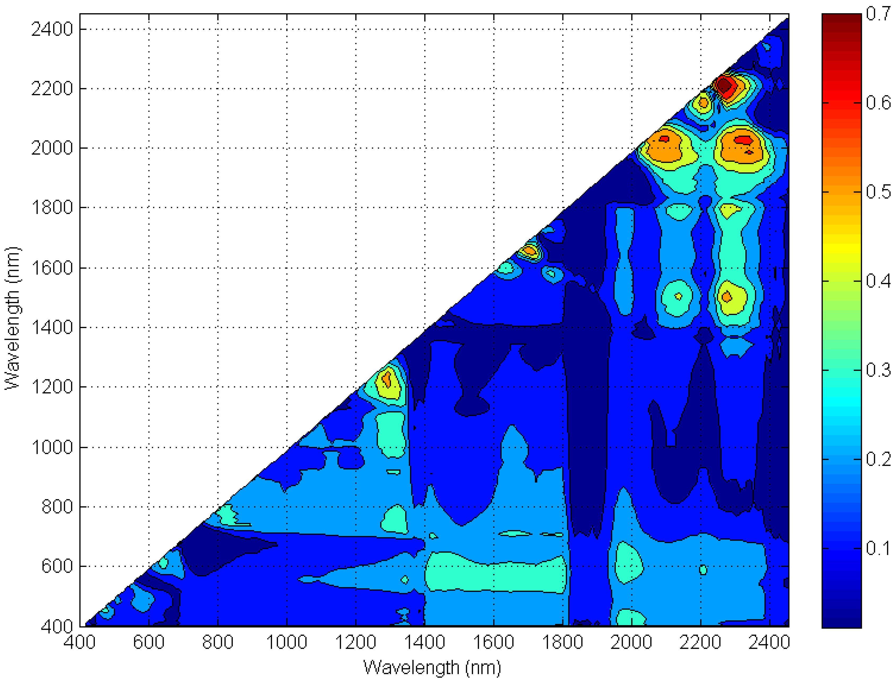
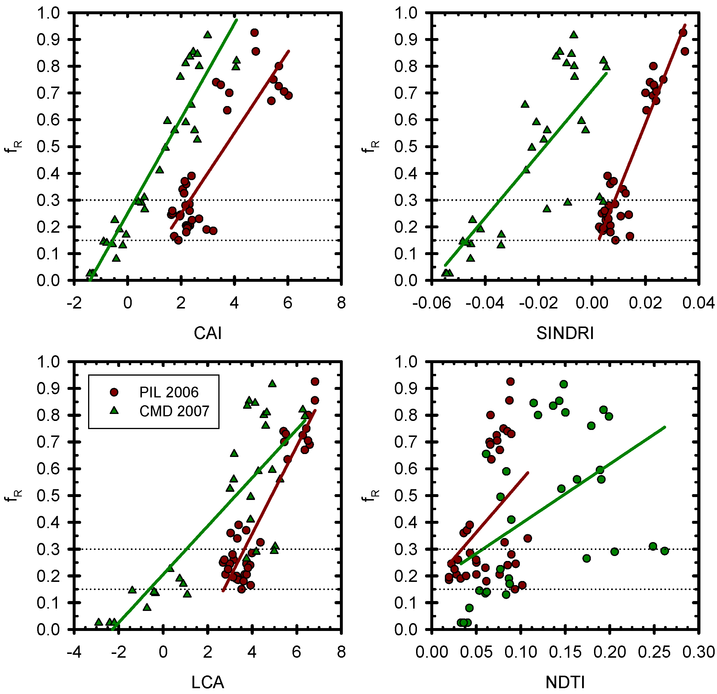
4.1. Hyperspectral and ASTER Index Determination

| FWHM bandwidth (nm) | 520–600 | 630–690 | 760–860 | 1600–1700 | 2145–2185 | 2185–2225 | 2235–2285 | 2295–2365 | 2360–2430 |
|---|---|---|---|---|---|---|---|---|---|
| ASTER band | 1 | 2 | 3 | 4 | 5 | 6 | 7 | 8 | 9 |
| 1 | - | ||||||||
| 2 | 0.173 | - | |||||||
| 3 | 0.101 | 0.104 | - | ||||||
| 4 | 0.298 | 0.257 | 0.239 | - | |||||
| 5 | 0.287 | 0.267 | 0.150 | 0.270 | - | ||||
| 6 | 0.289 | 0.273 | 0.159 | 0.206 | 0.495 | - | |||
| 7 | 0.284 | 0.267 | 0.149 | 0.362 | 0.557 | 0.741 | - | ||
| 8 | 0.269 | 0.266 | 0.154 | 0.342 | 0.298 | 0.456 | 0.140 | - | |
| 9 | 0.240 | 0.243 | 0.136 | 0.206 | 0.096 | 0.171 | 0.091 | 0.175 | - |


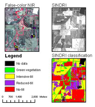
| 19 May 2007 | 27 May 2007 | |||||||||||||
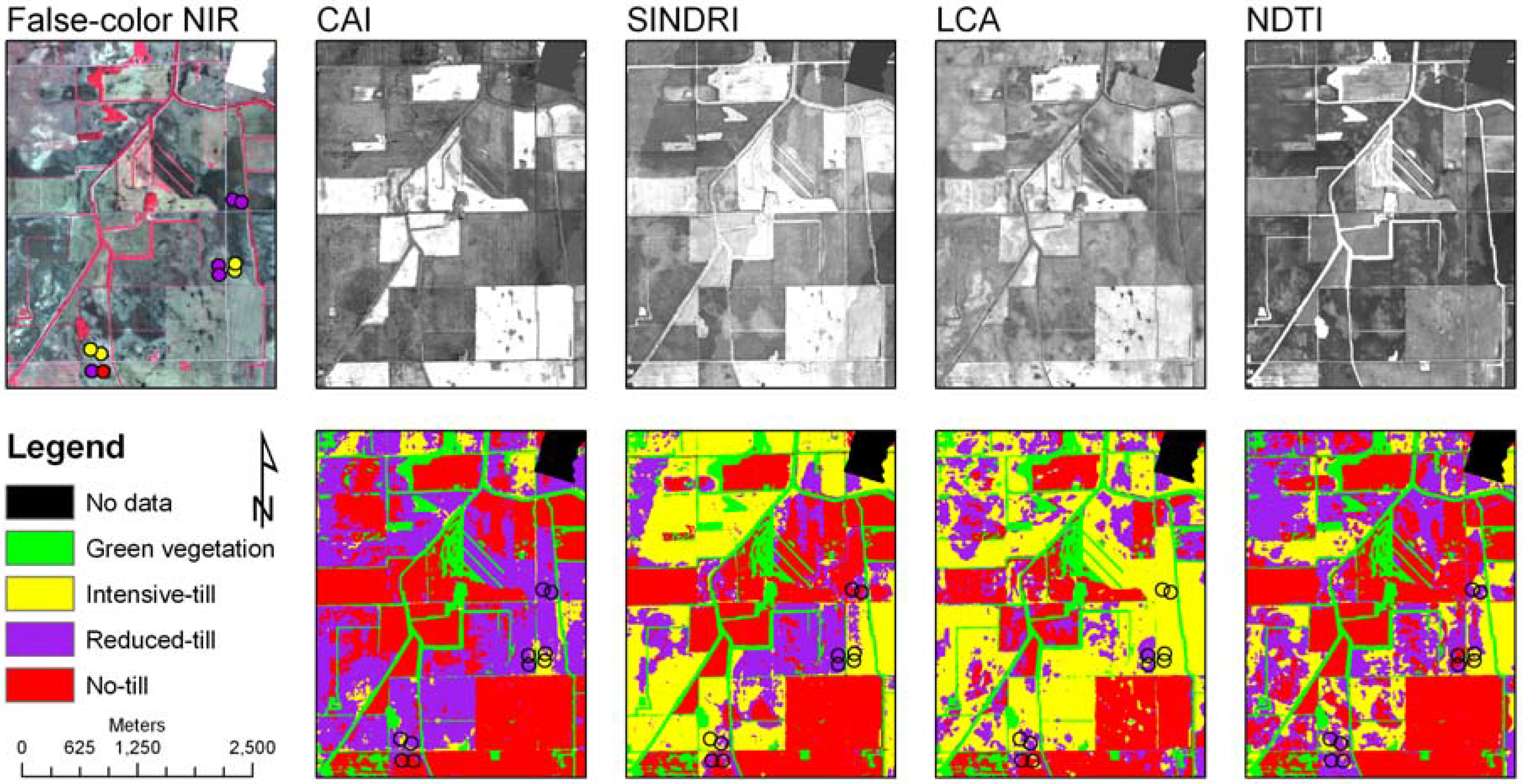
| Tillage class | SINDRI | LCA | NDTI | CAI | SINDRI | LCA | NDTI | |||||||
| Area (ha) | % | Area (ha) | % | Area (ha) | % | Area (ha) | % | Area (ha) | % | Area (ha) | % | Area (ha) | % | |
| Intensive | 843.8 | 7.9 | 443.9 | 4.1 | 1681.7 | 14.9 | 577.9 | 7.5 | 4285.6 | 55.3 | 660.6 | 8.5 | 0.0 | 0.0 |
| Reduced | 5941.5 | 55.5 | 4610.0 | 42.6 | 5280.1 | 46.8 | 6064.3 | 78.2 | 2819.9 | 36.4 | 4643.3 | 59.8 | 133.9 | 1.7 |
| Conserv. | 3918.2 | 36.6 | 5755.8 | 53.2 | 4310.8 | 38.2 | 1110.4 | 14.3 | 638.0 | 8.2 | 2461.8 | 31.7 | 7735.2 | 98.3 |

4.2. Effect of Water Content on Index Value
Conclusions
Acknowledgements
References and Notes
- Causarano, H.J.; Doraiswamy, P.C.; McCarty, G.W.; Hatfield, J.L.; Milak, S.; Stern, A.J. EPIC modeling of soil organic carbon sequestration in croplands of Iowa. J. Environ. Qual. 2008, 37, 1345–1353. [Google Scholar] [CrossRef] [PubMed]
- Causarano, H.J.; Franzluebbers, A.J.; Reeves, D.W.; Shaw, J.N. Soil organic carbon sequestration in cotton production systems of the southeastern United States: A review. J. Environ. Qual. 2006, 35, 1374–1383. [Google Scholar] [CrossRef] [PubMed]
- Monfreda, C.; Ramankutty, N.; Foley, J.A. Farming the planet: 2. Geographic distribution of crop areas, yields, physiological types, and net primary production in the year 2000. Global Biogeochem. Cycle 2008, 22, 1–19. [Google Scholar] [CrossRef]
- Ramankutty, N.; Evan, A.T.; Monfreda, C.; Foley, J.A. Farming the planet: 1. Geographic distribution of global agricultural lands in the year 2000. Global Biogeochem. Cycle 2008, 22, GB1003. [Google Scholar] [CrossRef]
- Archer, D.W.; Halvorson, A.D.; Reule, C.A. Economics of irrigated continuous corn under Conventional-Till and No-Till in Northern Colorado. Agron. J. 2008, 100, 1166–1172. [Google Scholar] [CrossRef]
- Paudel, K.P.; Lohr, L.; Cabrera, M. Residue management systems and their implications for production efficiency. Renew. Agr. Food Syst. 2006, 21, 124–133. [Google Scholar] [CrossRef]
- McGinnis, L. Show me the money: Why economics is essential for sustainable agriculture. Agr. Res. 2007, 55, 8–11. [Google Scholar]
- Lal, R. World crop residues production and implications of its use as a biofuel. Environ. Int. 2005, 31, 575–584. [Google Scholar] [PubMed]
- Laflen, J.M.; Amemiya, M.; Hintz, E.A. Measuring crop residue cover. J. Soil Water Conserv. 1981, 36, 341–343. [Google Scholar]
- Morrison, J.E., Jr.; Huang, C.H.; Lightle, D.T.; Daughtry, C.S.T. Residue measurement techniques. J. Soil Water Conserv. 1993, 48, 479–483. [Google Scholar]
- Daughtry, C.S.T. Discriminating crop residues from soil by shortwave infrared reflectance. Agron. J. 2001, 93, 125–131. [Google Scholar] [CrossRef]
- Daughtry, C.S.T.; Hunt, E.R., Jr.; Doraiswamy, P.C.; McMurtrey, J.E., III. Remote sensing the spatial distribution of crop residues. Agron. J. 2005, 97, 864–871. [Google Scholar] [CrossRef]
- McNairn, H.; Protz, R. Mapping corn residue cover on agricultural fields in Oxford County, Ontario, using Thematic Mapper. Can. J. Remote Sens. 1993, 19, 152–159. [Google Scholar] [CrossRef]
- van Deventer, A.P.; Ward, A.P.; Gowda, P.H.; Lyon, J.G. Using Thematic Mapper data to identify contrasting soil plains to tillage practices. Photogramm. Eng. Remote Sens. 1997, 63, 87–93. [Google Scholar]
- Qi, J.; Marsett, R.; Heilman, P.; Biedenbender, S.; Moran, S.; Goodrich, D.; Weltz, M. RANGES improves satellite-based information and land cover assessments in southwest United States. Eos 2002, 83, 601–606. [Google Scholar] [CrossRef]
- Biard, F.; Baret, F. Crop residue estimation using multiband reflectance. Remote Sens. Environ. 1997, 59, 530–536. [Google Scholar] [CrossRef]
- Serbin, G.; Daughtry, C.S.T.; Hunt, E.R., Jr.; Brown, D.J.; McCarty, G.W. Effect of soil spectral properties on remote sensing of crop residue cover. Soil Sci. Soc. Am. J. 2009, 73, 1545–1558. [Google Scholar] [CrossRef]
- Brown, D.J.; Shepherd, K.D.; Walsh, M.G.; Mays, M.D.; Reinsch, T.G. Global soil characterization with VNIR diffuse reflectance spectroscopy. Geoderma 2006, 132, 273–290. [Google Scholar] [CrossRef]
- U. S. Geological Survey USGS EO-1 Website. Available online: http://eo1.usgs.gov/hyperion.php (accessed 25 August 2009).
- Gill, T.K.; Phinn, S.R. Estimates of bare ground and vegetation cover from Advanced Spaceborne Thermal Emission and Reflection Radiometer (ASTER) short-wave-infrared reflectance imagery. J. Appl. Remote Sens. 2008, 2, 023511. [Google Scholar] [CrossRef] [Green Version]
- Gill, T.K.; Phinn, S.R. Improvements to ASTER-derived fractional estimates of bare ground in a savanna rangeland. IEEE Trans. Geosci. Remote Sens. 2009, 47, 662–670. [Google Scholar] [CrossRef]
- Chikhaoui, M.; Bonn, F.; Bokoye, A.I.; Merzouk, A. A spectral index for land degradation mapping using ASTER data: Application to a semi-arid Mediterranean catchment. Int. J. Appl. Earth Obs. Geoinformation 2005, 7, 140–153. [Google Scholar] [CrossRef]
- Lewis, D.; Yao, H.; Fridgen, J.; Kincaid, R. Investigation on the Potential of using ASTER Image for Corn Plant Residue Coverage Estimation in Three Indiana Counties. In 2006 IEEE International Geoscience & Remote Sensing Symposium IGARSS’06; IEEE Geoscience and Remote Sensing Society: Denver, CO, USA, 2006; pp. 2092–2094. [Google Scholar]
- NASA Jet Propulsion Laboratory SWIR—ASTER User Advisory. Available online: http://asterweb.jpl.nasa.gov/swir-alert.asp (accessed 7 July, 2009).
- Baumgardner, M.F.; Silva, L.F.; Biehl, L.L.; Stoner, E.R. Reflectance properties of soils. In Advances in Agronomy; Volume 38, Brady, N.C., Ed.; Academic Press, Inc.: New York, NY, USA, 1985; pp. 2–44. [Google Scholar]
- Clark, R.N. Spectroscopy of rocks and minerals, and principles of spectroscopy. In Manual of Remote Sensing, Volume 3, Remote Sensing for the Earth Sciences; Rencz, A.N., Ed.; John Wiley and Sons: New York, NY, USA, 1999; pp. 3–58. [Google Scholar]
- Clark, R.N.; Swayze, G.A.; Livo, K.E.; Kokaly, R.F.; Sutley, S.J.; Dalton, J.B.; McDougal, R.R.; Gent, C.A. Imaging spectroscopy: Earth and planetary remote sensing with the USGS Tetracorder and expert systems. J. Geophys. Res. Planets 2003, 108, 5131. [Google Scholar] [CrossRef]
- Stoner, E.R.; Baumgardner, M.F. Characteristic variations in reflectance of surface soils. Soil Sci. Soc. Am. J. 1981, 45, 1161–1165. [Google Scholar] [CrossRef]
- Waiser, T.H.; Morgan, C.L.S.; Brown, D.J.; Hallmark, C.T. In situ characterization of soil clay content with visible near-infrared diffuse reflectance spectroscopy. Soil Sci. Soc. Am. J. 2007, 71, 389–396. [Google Scholar] [CrossRef]
- Daughtry, C.S.T.; Hunt, E.R., Jr. Mitigating the effects of soil and residue water contents on remotely sensed estimates of crop residue cover. Remote Sens. Environ. 2008, 112, 1647–1657. [Google Scholar] [CrossRef]
- Lobell, D.B.; Asner, G.P. Moisture effects on soil reflectance. Soil Sci. Soc. Am. J. 2002, 66, 722–727. [Google Scholar] [CrossRef]
- Nagler, P.L.; Daughtry, C.S.T.; Goward, S.N. Plant litter and soil reflectance. Remote Sens. Environ. 2000, 71, 207–215. [Google Scholar] [CrossRef]
- Whiting, M.L.; Li, L.; Ustin, S.L. Predicting water content using Gaussian model on soil spectra. Remote Sens. Environ. 2004, 89, 535–552. [Google Scholar] [CrossRef]
- Serbin, G.; Daughtry, C.S.T.; Hunt, E.R., Jr.; McCarty, G.W.; Doraiswamy, P.C.; Brown, D.J. Improved remotely-sensed estimates of crop residue cover by incorporating soils information. In 2008 IEEE International Geoscience & Remote Sensing Symposium IGARSS’08; IEEE Geoscience and Remote Sensing Society: Boston, MA, USA, 2008. [Google Scholar]
- Salisbury, J.W.; Hunt, G.R. Martian surface materials: effect of particle size on spectral behavior. Science 1968, 161, 365–366. [Google Scholar] [CrossRef] [PubMed]
- Ben-Dor, E.; Goldlshleger, N.; Benyamini, Y.; Agassi, M.; Blumberg, D.G. The spectral properties of soil structural crusts in the 1.2- to 2.5-μm spectral region. Soil Sci. Soc. Am. J. 2003, 67, 289–299. [Google Scholar] [CrossRef]
- Ben-Dor, E. Quantitative remote sensing of soil properties. In Advances in Agronomy; Volume 75, Sparks, D., Ed.; Academic Press: San Diego, CA, USA, 2002; pp. 173–244. [Google Scholar]
- Ben-Dor, E.; Chabrillat, S.; Demattê, J.A.M.; Taylor, G.R.; Hill, J.; Whiting, M.L.; Sommer, S. Using Imaging Spectroscopy to study soil properties. Remote Sens. Environ. 2009, 113, S38–S55. [Google Scholar] [CrossRef]
- Green, R.O. Measuring the spectral expression of carbon dioxide in the solar reflected spectrum with AVIRIS. In Tenth Annual JPL Airborne Earth Science Workshop; California Institute of Technology Jet Propulsion Laboratory: Pasadena, CA, USA, 2001. [Google Scholar]
- Workman, J., Jr.; Weyer, L. Practical Guide to Interpretive Near-Infrared Spectroscopy; Taylor & Francis Group: Boca Raton, FL, USA, 2008; p. 332. [Google Scholar]
- Elvidge, C.D. Visible and near infrared reflectance characteristics of dry plant materials. Int. J. Remote Sens. 1990, 11, 1775–1795. [Google Scholar] [CrossRef]
- Kokaly, R.F.; Clark, R.N. Spectroscopic determination of leaf biochemistry using band-depth analysis of absorption features and stepwise multiple linear regression. Remote Sens. Environ. 1999, 67, 267–287. [Google Scholar] [CrossRef]
- Serbin, G.; Daughtry, C.S.T.; Hunt, E.R., Jr.; Reeves, J.B., III; Brown, D.J. Effects of soil composition and mineralogy on remote sensing of crop residue cover. Remote Sens. Environ. 2009, 113, 224–238. [Google Scholar] [CrossRef]
- Sabins, F.F., Jr. Remote Sensing: Principles and Interpretation, 2nd edition; W. H. Freeman and Company: New York, NY, USA, 1987; p. 449. [Google Scholar]
- U. S. Geological Survey Spectral Characteristics Viewer. http://landsat.usgs.gov/tools_viewer.php (accessed 7 August 2009).
- Ritchie, S.W.; Hanway, J.J.; Benson, G.O. How a Corn Plant Develops, Special Report No. 48; Iowa State University of Science and Technology Cooperative Extension Service: Ames, IA, USA, 2005; p. 21. [Google Scholar]
- Yale University Center for Earth Observation ASTER. Available online: http://www.yale.edu/ceo/Documentation/ASTER.pdf (accessed 7 August 2009).
- NASA Goddard Space Flight Center The Landsat Program. Available online: http://landsat.gsfc.nasa.gov/ (accessed 16 August 2009).
- Sherrod, L.A.; Dunn, G.; Peterson, G.A.; Kolberg, R.L. Inorganic carbon analysis by modified pressure-calcimeter method. Soil Sci. Soc. Am. J. 2002, 66, 299–305. [Google Scholar] [CrossRef]
- Rouse, J.W., Jr.; Haas, R.H.; Deering, D.W.; Schell, J.A. Monitoring the vernal advancement and retrogradation (green wave effect) of natural vegetation; Texas A&M University: College Station, TX, USA, 1973; p. 93. [Google Scholar]
- Congalton, R.G.; Green, K. Assessing the Accuracy of Remotely Sensed data: Principles and Practices, 2nd Ed. ed; CRC Press: Boca Raton, FL, USA, 2009; p. 183. [Google Scholar]
- Conservation Technology Information Center 2009 CTIC Crop Residue Management Survey System. Available online: http://www.crmsurvey.org/ (accessed 12 August 2009).
- National Weather Service. Record of Evaporation and Climatological Observations Ames 8 WSW; NOAA National Weather Service National Climatic Data Center: Silver Spring, MD, USA, May 2007. [Google Scholar]
- Hunt, E.R., Jr.; Rock, B.N. Detection of changes in leaf water content using near- and middle-infrared reflectances. Remote Sens. Environ. 1989, 30, 43–54. [Google Scholar]
- Morrison, J.E.; Rickman, R.W.; McCool, D.K.; Pfeiffer, K.L. Measurement of wheat residue cover in the Great Plains and Pacific Northwest. J. Soil Water Conserv. 1997, 52, 59–65. [Google Scholar]
© 2009 by the authors; licensee Molecular Diversity Preservation International, Basel, Switzerland. This article is an open-access article distributed under the terms and conditions of the Creative Commons Attribution license (http://creativecommons.org/licenses/by/3.0/).
Share and Cite
Serbin, G.; Hunt, E.R., Jr.; Daughtry, C.S.T.; McCarty, G.W.; Doraiswamy, P.C. An Improved ASTER Index for Remote Sensing of Crop Residue. Remote Sens. 2009, 1, 971-991. https://doi.org/10.3390/rs1040971
Serbin G, Hunt ER Jr., Daughtry CST, McCarty GW, Doraiswamy PC. An Improved ASTER Index for Remote Sensing of Crop Residue. Remote Sensing. 2009; 1(4):971-991. https://doi.org/10.3390/rs1040971
Chicago/Turabian StyleSerbin, Guy, E. Raymond Hunt, Jr., Craig S. T. Daughtry, Gregory W. McCarty, and Paul C. Doraiswamy. 2009. "An Improved ASTER Index for Remote Sensing of Crop Residue" Remote Sensing 1, no. 4: 971-991. https://doi.org/10.3390/rs1040971