Estimating Flow Resistance of Wetlands Using SAR Images and Interaction Models

Abstract
:1. Introduction
2. Study Area
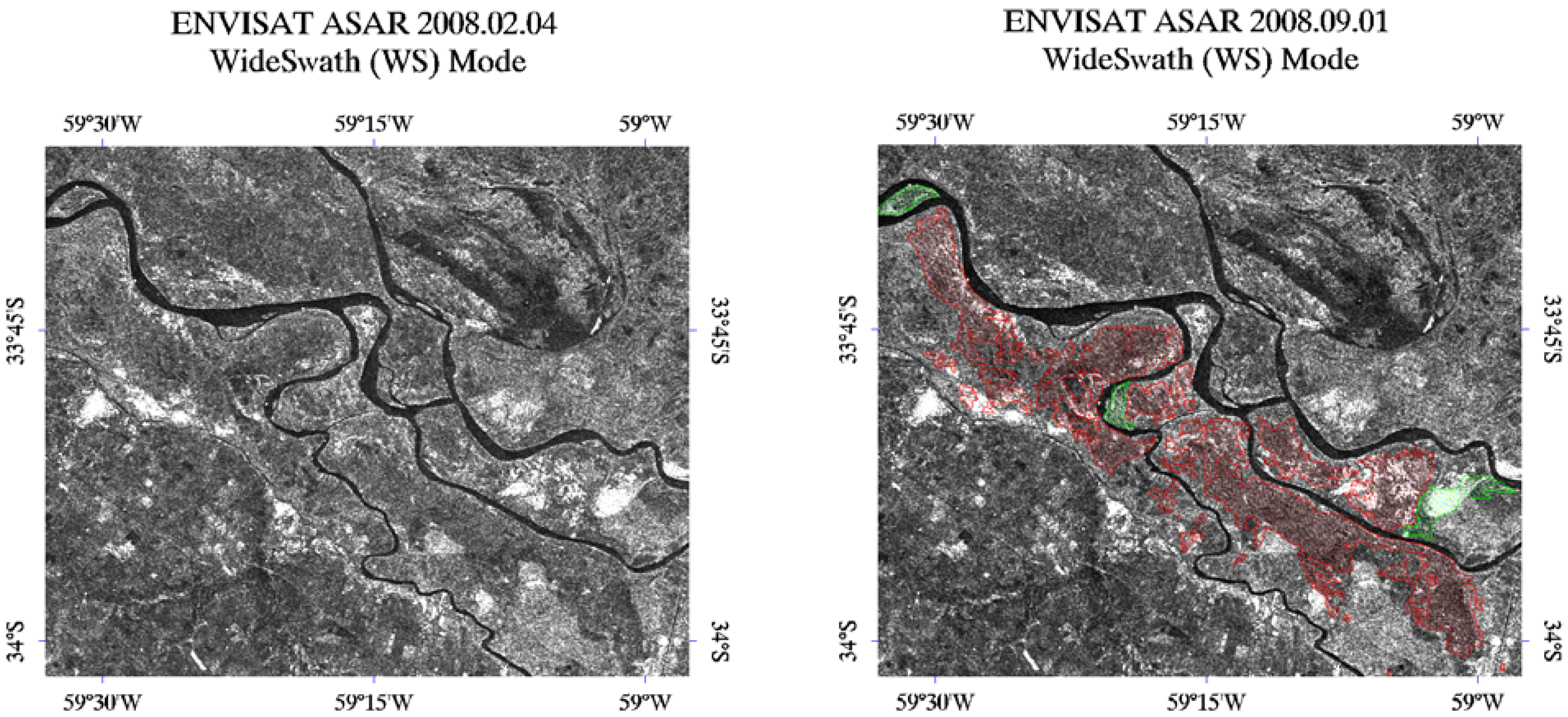
2.1. Fire Event
3. Satellite Data Sets and Fieldwork

| Parameter | Value | |
|---|---|---|
| SAC-C/MMRS | Number of spectral bands | 5 |
| Spectral range | 480–1,700 nm | |
| Spatial resolution | 175 m | |
| Radiometric resolution | 8 bits | |
| Swath Wide | 360 Km | |
| Envisat ASAR | Mode | Wide Swath (Scan SAR) |
| Spatial resolution | 75 m | |
| Swath Wide | 400 Km | |
| Central frequency | 5.3 GHz (C Band) | |
| Polarization | HH | |
| Incidence angle | 19°–45° | |
| Equivalent Number of Looks (ENL) | ~21 |
4. Methodology


4.1. Estimation of the Reduction of Junco Plant Density


4.1.1. The interaction model
| Parameter | Value | Comments |
| Frequency | 5.3 GHz | Envisat ASAR |
| Incidence angle | 19º–40º | ASAR WS (near range/far range) |
| Soil RMS height | 0.1 cm | Flooded soil. |
| Soil correlation length | 10 cm | Flooded soil. |
| Gravimetric soil moisture | 0.35 g/g | Saturated marsh soil. From field data. |
| Junco plant diameter | 0.7 cm | Mean value. From field data. |
| Junco plant gravimetric moisture | 0.7 g/g | Mean value. From field data. |
| Junco plant height | 180 cm | Mean value. From field data. |
| Junco plant angular distribution | Non-uniform | see [14] |
| Junco plant density | Variable | Dependent on fire disturbance |

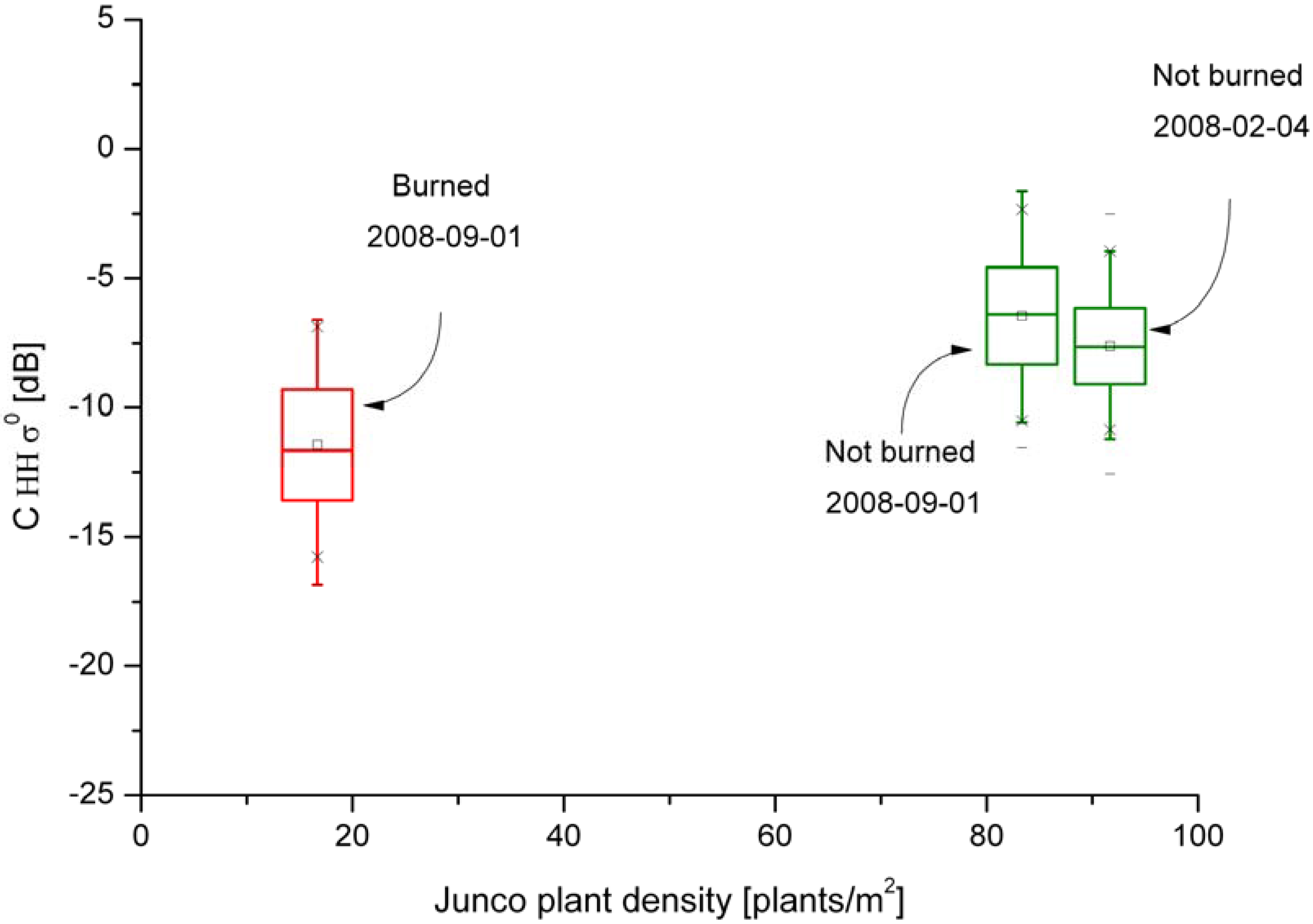
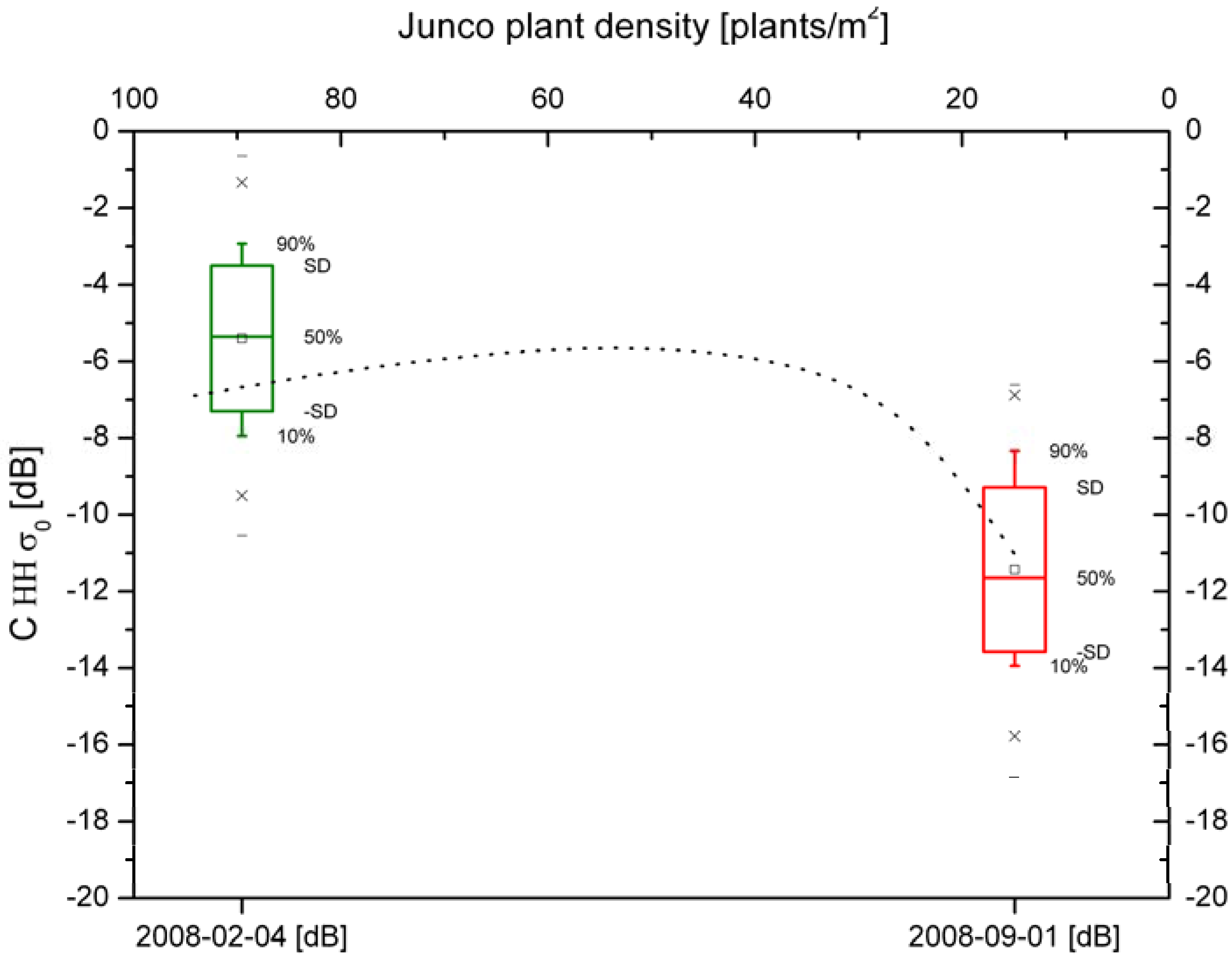
- The interaction model generally reproduces the observed σ0 values of junco marsh corresponding to extreme values of JPD (box plots red and green).
- The interaction model predicts a rapid increase of the total σ0 as function of JPD, related to an increase in junco marsh radar cross section reaching a maximum at about 40 plants/m2. Then, the HH σ0 trend becomes flat and shows almost no sensitivity to JPD changes. This can be explained considering that the junco marsh total σ0 can be considered a balance between soil-junco double bounce interaction and Junco extinction [6]. An increase in JPD means additional junco plants available for backscattering, but also more junco plants for extinction. The complex balance between these two magnitudes depends strongly on vegetation structure and dielectric properties (see [6] for a complete discussion about junco marsh scattering behaviour).
- Finally, this simulation can be used to estimate remaining JPD as a function of HH σ0, at least for low values of JPD.
4.2. Estimation of the Junco Marsh Hydraulic Conductivity
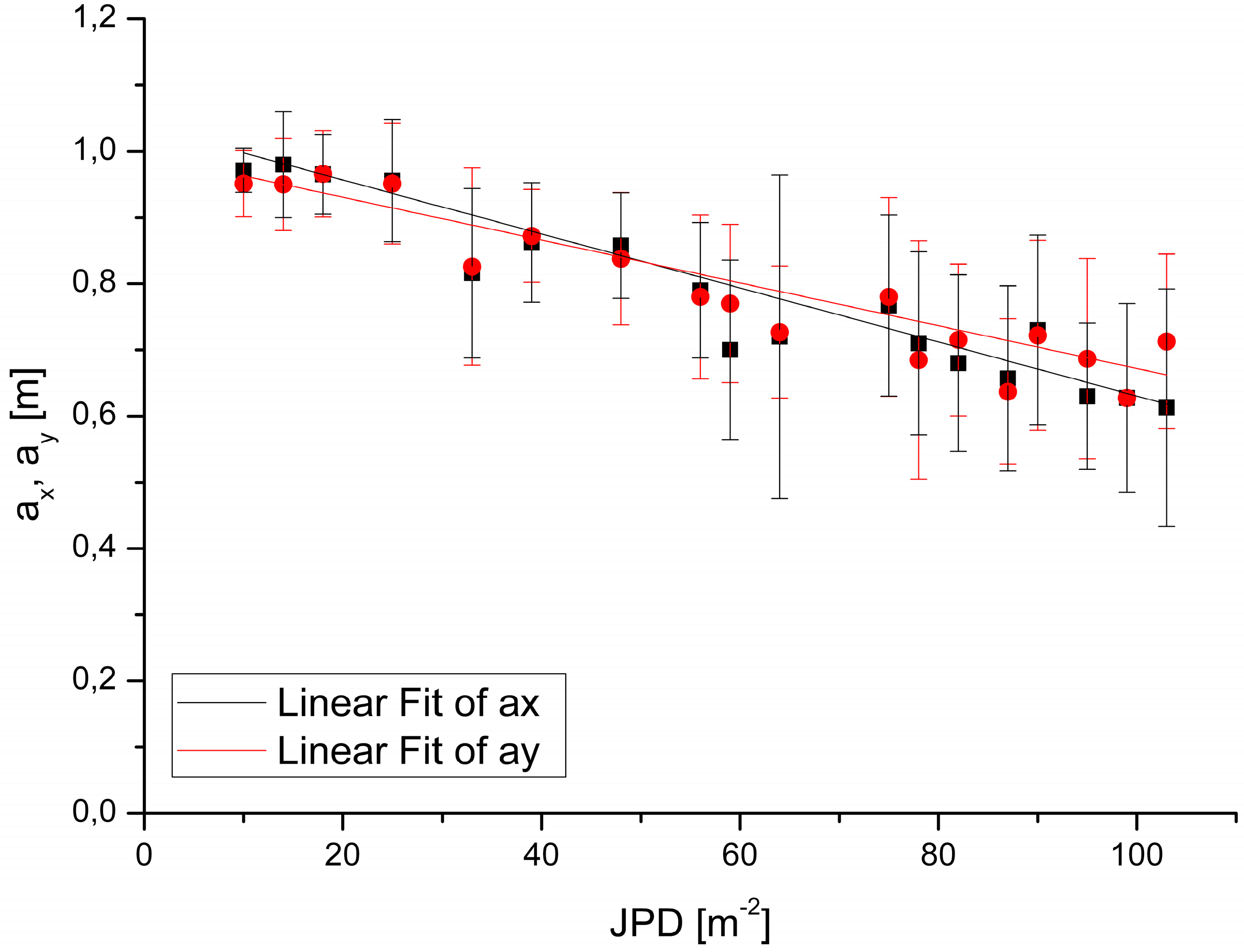
- ax and ay depend implicitly on vegetation spatial distribution and
- the only dynamical-dependent input of Equation (3) is Cd∞, the drag coefficient of a single cylinder.
- Junco shoots can be considered as rigid circular cylinders. Actually, junco shoots are flexible, but its flexibility is only important at large water velocities [23].
- The flux is stationary (∂u/∂t = 0). This means that the input flux to the channel does not vary with time.
- The Reynolds number of the problem is low.

4.3. Estimation of Junco Marsh Patch Drag Coefficient
| HH σ0 | Estimated JPD [m–2] | Single plant Cd | Estimated junco marsh Cd | Area [ha] |
|---|---|---|---|---|
| <−11 dB | <15 plants/m2 | <1.65 | <25 | 16,594 (68.9 %) |
| –10 dB < σ0 < –11 dB | 15–20 plants/m2 | 1.69 | 25–34 | 3,675 (15.3 %) |
| –9 dB < σ0 < –10 dB | 20–25 plants/m2 | 1.73 | 34–43 | 1,943 (8.1 %) |
| –8 dB < σ0 < –9 dB | 25–30 plants/m2 | 1.77 | 43–54 | 968 (4.1 %) |
| –7 dB < σ0 < –8 dB | 30–35 plants/m2 | 1.81 | 54–65 | 532 (2.2 %) |
| –6 dB < σ0 < –7 dB | 35–40 plants/m2 | 1.86 | 65–76 | 357 (1.5 %) |
| >–6 dB | >40 plants/m2 | >1.9 | >76 | 161 (0.7 %) |
5. Results

6. Discussion
- The junco drag coefficient map presents areas with low and high spatial homogeneity. This is typical of burning events in wetlands; where the access to fuel and the presence of water usually leads to a heterogeneous burning pattern. This heterogeneity is not related to the speckle phenomena, since (i) ENL is high and (ii) the speckle phenomenon is expected to affect the whole image.
- Areas where islands are larger (and cattle raising is more common), were the most affected both in intensity and homogeneity (Cd ≈ 25 or less, red in the map).
- Areas in the middle part of the Paraná River Delta were less homogeneously affected, due to the intrinsic heterogeneity of the vegetation and the water channels present in the area.
- Values presented in blue (class coastal) correspond to coastal junco marsh patches located at the island line coast that present a higher backscattering coefficient due to a different flood state. Therefore, they will be excluded from our analysis.
- Table 3 shows that most of the burned area corresponds to completely destroyed junco marsh patches (<15 plants/m2), as expected from the information obtained using optical images and field data. This implies that fire events reduced drastically the wetland overall drag coefficient in this area. This should have important effects in the future behaviour of Paraná’s River seasonal flooding, reducing water resilient time and increasing water level peak.
7. Conclusions
Acknowledgements
References and Notes
- Järvelä, J. Influence of vegetation on flow structure in floodplains and wetlands. In 3rd IAHR Symposium on River, Coastal and Estuarine Morphodynamics, Madrid, Spain, 1–5 September 2003; pp. 845–856.
- Järvelä, J. Flow resistance in environmental channels: focus on vegetation. In Helsinki University of Technology Water Resources Publications (ISBN 951-22-7073-0), TKK-VTR-10; Helsinki University of Technology, Laboratory of Water Resources: Espoo, Filand, 2004. [Google Scholar]
- Alsdorf, D.E.; Melack, J.M.; Dunne, T.; Mertes, L.A.K.; Hess, L.L.; Smith, L.C. Interferometric radar measurements of water level changes on the Amazon flood plain. Nature 2000, 404, 174–177. [Google Scholar] [CrossRef] [PubMed]
- Grings, F.; Salvia, M.; Karszenbaum, H.; Ferrazzoli, P.; Kandus, P.; Perna, P. Exploring the capacity of radar to estimate Wetland Marshes Water Storage. J. Environ. Manage. 2009, 90, 2189–2198. [Google Scholar] [CrossRef] [PubMed]
- Kasischke, E.; Melack, J.; Dobson, M. The use of imaging radars for ecological applications—a review. Remote Sens. Environ. 1997, 59, 141–156. [Google Scholar] [CrossRef]
- Grings, F.M.; Ferrazzoli, P.; Jacobo-Berlles, J.C.; Karszenbaum, H.; Tiffenberg, J.; Pratolongo, P.; Kandus, P. Monitoring flood condition in marshes using EM models and Envisat ASAR observations. IEEE Trans. Geosci. Remote Sens. 2006, 44, 936–942. [Google Scholar] [CrossRef]
- Pope, K.O.; Rejmankova, E.; Paris, F.F.; Woodruff, R. Detecting seasonal flooding cycles in marshes of the Yucatan peninsula with SIR-C polarimetric radar imagery. Remote Sens. Environ. 1997, 59, 157–166. [Google Scholar] [CrossRef]
- Kandus, P.; Málvarez, A.I.; Madanes, N. Study on the herbaceous plant communities in the Lower Delta islands of the Paraná River (Argentina). Darwiniana 2003, 41, 1–16. [Google Scholar]
- Salvia, M.; Karszenbaum, H.; Grings, F.; Kandus, P. Datos satelitales ópticos y de radar para el mapeo de ambientes en macrosistemas de humedal. Rev.Teledetec. 2009, 31, 35–51. [Google Scholar]
- Grings, F.; Ferrazzoli, P.; Karszenbaum, H.; Tiffenberg, J.; Kandus, P.; Guerriero, L.; Jacobo-Berrles, J. Modeling temporal evolution of junco marshes radar signatures. IEEE Trans. Geosci. Remote Sens. 2005, 43, 2238–2245. [Google Scholar] [CrossRef]
- Stamati, M.; Bono, J.; Parmuchi, M.G.; Salvia, M.; Strada, M.; Montenegro, C.; Kandus, P.; Menéndez, J.; Karszenbaum, H. Evaluación de la superficie afectada por los incendios ocurridos en el Delta del río Paraná en abril de 2008. Poster presentation. In XXIII Reunión Argentina de Ecología, Investigación ecológica: avances y desafíos, San Luis, Argentina, 25–28 November 2008.
- Bonetto, A.A.; Wais, J.R.; Castello, H.P. The increasing damming of the Paraná basin and its effects on the lower reaches. Regul. River. 2006, 4, 333–346. [Google Scholar] [CrossRef]
- RAMSAR Convention Secretariat. Water-related guidance: an Integrated Framework for the Convention’s water-related guidance. In Ramsar Handbooks for the Wise Use of Wetlands, 3rd ed.; Ramsar Convention Secretariat: Gland, Switzerland, 2002; Volume 6. [Google Scholar]
- Coe, M.T. Modelling terrestrial hydrological systems at the continental scale: testing the accuracy of an atmospheric GCM. J. Clim. 2000, 13, 686–704. [Google Scholar] [CrossRef]
- Grings, F.; Ferrazzoli, P.; Karszenbaum, H.; Salvia, M.; Kandus, P.; Jacobo-Berlles, J.C.; Perna, P. Model investigation about the potential of C band SAR in herbaceous wetlands flood monitoring. Int. J. Remote Sens. 2008, 29, 5361–5372. [Google Scholar] [CrossRef]
- ESA. ASAR Handbook. 1995. Available online: http://envisat.esa.int/handbooks/asar/ (accessed on 15 August 2008).
- Patel, P.; Srivastava, H.S.; Panigrahy, S.; Parihar, J.S. Comparative evaluation of the sensitivity of multi-polarized multi-frequency SAR backscatter to plant density. Int. J. Remote Sens. 2006, 2, 293–305. [Google Scholar] [CrossRef]
- Della Vecchia, A.; Ferrazzoli, P.; Guerriero, L.; Blaes, X.; Defourny, P.; Dente, L.; Mattia, F.; Satalino, G.; Strozzi, T.; Wegmuller, U. Influence of geometrical factors on crop backscattering at C-band. IEEE Trans. Geosci. Remote Sens. 2006, 44, 778–790. [Google Scholar] [CrossRef]
- Bracaglia, M.; Ferrazzoli, P.; Guerriero, L. A fully polarimetric multiple scattering model for crops. Remote Sens. Environ. 1995, 54, 170–179. [Google Scholar] [CrossRef]
- Fung, A.K. Microwave Scattering and Emission Models and Their Applications; Artech House: Norwood, OH, USA, 1994. [Google Scholar]
- Karam, M.A.; Fung, A.K. Electromagnetic scattering from a layer of finite length, randomly oriented, dielectric, circular cylinders over a rough interface with application to vegetation. Int. J. Remote Sens. 1998, 9, 1109–1134. [Google Scholar] [CrossRef]
- El-Rayes, M.A.; Ulaby, F.T. Microwave dielectric spectrum of vegetation—Part I: Experimental observations. IEEE Trans. Geosci. Remote Sens. 1987, 25, 541–549. [Google Scholar] [CrossRef]
- Järvelä, J. Determination of flow resistance caused by non-submerged woody vegetation. Int. J. River Manag. 2004, 2, 61–70. [Google Scholar] [CrossRef]
- Nepf, H.; Koch, E. Vertical secondary flows in submersed plant-like arrays. Limnol. Oceanogr. 1999, 44, 1072–1080. [Google Scholar] [CrossRef]
- Lindner, K. Der Strömungswiderstand von Pflanzenbeständen. PhD dissertation, Leichtweiss-Institut für Wasserbau, Technische Universität Braunschweig, Pfaffenwaldring 61 70569 Stuttgart, Germany, 1982. [Google Scholar]
- Oldham, C.; Sturman, J. The effect of emergent vegetation on convective flushing in shallow wetlands: Scaling and experiments. Limnol. Oceanogr. 2001, 46, 1486–1493. [Google Scholar] [CrossRef]
- Stone, B.M.; Shen, H.T. Hydraulic resistance of flow in channels with cylindrical roughness. J. Hydr. Engrg. 2002, 128, 500–506. [Google Scholar] [CrossRef]
- Patel, P.; Srivastava, H.S.; Navalgund, R.R. Use of synthetic aperture radar polarimetry to characterize wetland targets of Keoladeo National Park, Bharatpur, India. Curr. Sci. 2009, 97, 529–537. [Google Scholar]
© 2009 by the authors; licensee Molecular Diversity Preservation International, Basel, Switzerland. This article is an open-access article distributed under the terms and conditions of the Creative Commons Attribution license (http://creativecommons.org/licenses/by/3.0/).
Share and Cite
Salvia, M.; Franco, M.; Grings, F.; Perna, P.; Martino, R.; Karszenbaum, H.; Ferrazzoli, P. Estimating Flow Resistance of Wetlands Using SAR Images and Interaction Models. Remote Sens. 2009, 1, 992-1008. https://doi.org/10.3390/rs1040992
Salvia M, Franco M, Grings F, Perna P, Martino R, Karszenbaum H, Ferrazzoli P. Estimating Flow Resistance of Wetlands Using SAR Images and Interaction Models. Remote Sensing. 2009; 1(4):992-1008. https://doi.org/10.3390/rs1040992
Chicago/Turabian StyleSalvia, Mercedes, Mariano Franco, Francisco Grings, Pablo Perna, Roman Martino, Haydee Karszenbaum, and Paolo Ferrazzoli. 2009. "Estimating Flow Resistance of Wetlands Using SAR Images and Interaction Models" Remote Sensing 1, no. 4: 992-1008. https://doi.org/10.3390/rs1040992