Disaggregation of Landsat-8 Thermal Data Using Guided SWIR Imagery on the Scene of a Wildfire


Department of Civil and Environmental Engineering, Seoul National University, 1, Gwanak-ro, Gwanak-gu, Seoul 08826, Korea
*
Author to whom correspondence should be addressed.
Remote Sens. 2018, 10(1), 105; https://doi.org/10.3390/rs10010105
Submission received: 29 October 2017
/
Revised: 13 December 2017
/
Accepted: 10 January 2018
/
Published: 13 January 2018
(This article belongs to the Special Issue Remote Sensing for Land Surface Temperature (LST) Estimation, Generation, and Analysis)
Abstract
:Thermal data products derived from remotely sensed data play significant roles as key parameters for biophysical phenomena. However, a trade-off between spatial and spectral resolutions has existed in thermal infrared (TIR) remote sensing systems, with the end product being the limited resolution of the TIR sensor. In order to treat this problem, various disaggregation methods of TIR data, based on the indices from visible and near-infrared (VNIR), have been developed to sharpen the coarser spatial resolution of TIR data. Although these methods were reported to exhibit sufficient performance in each study, preservation of thermal variation in the original TIR data is still difficult, especially in fire areas due to the distortion of the VNIR reflectance by the impact of smoke. To solve this issue, this study proposes an efficient and improved disaggregation algorithm of TIR imagery on wildfire areas using guided shortwave infrared (SWIR) band imagery via a guided image filter (GF). Radiometric characteristics of SWIR wavelengths could preserve spatially high frequency temperature components in flaming combustion, and the GF preserved thermal variation of the original TIR data in the disaggregated result. The proposed algorithm was evaluated using Landsat-8 operational land imager (OLI) and thermal infrared sensor (TIRS) images on wildfire areas, and compared with other algorithms based on a vegetation index (VI) originating from VNIR. In quantitative analysis, the proposed disaggregation method yielded the best values of root mean square error (RMSE), mean absolute error (MAE), correlation coefficient (CC), erreur relative globale adimensionelle de synthèse (ERGAS), and universal image quality index (UIQI). Furthermore, unlike in other methods, the disaggregated temperature map in the proposed method reflected the thermal variation of wildfire in visual analysis. The experimental results showed that the proposed algorithm was successfully applied to the TIR data, especially to wildfire areas in terms of quantitative and visual assessments.
1. Introduction
Thermal data is related to emissivity of objects on the ground, and this property can account for biophysical phenomena [1,2]. Recently, thermal remote sensing based on satellite sensors has made it possible to establish temperature maps over wide areas. However, a trade-off exists between spatial and spectral resolutions in any spaceborne remote sensing system [3,4]. This limitation appears especially in thermal infrared (TIR) sensors. For instance, TIR sensors in the Landsat-8 platform obtain the radiation emitted by the earth in a range of 10–13 μm, but the TIR band retrieves lower total radiation than visible-near infrared (VNIR) and shortwave infrared (SWIR) bands. Due to this radiometric characteristic of the TIR sensor, the spatial resolution of the TIR band is coarser than that of other bands. In addition, the limited spatial resolution of TIR sensors emphasizes the necessity for disaggregation of TIR imagery, also called thermal sharpening or downscaling, in order to improve the spatial resolution of the thermal data products [5]. The purpose of TIR disaggregation is to sharpen the coarser spatial resolution of TIR images by introducing spatial detail from a finer resolution multispectral (MS) image, without distortion of spectral information.
To achieve this purpose, various disaggregation methods of TIR imagery have been proposed in the last few decades. Generally, most have been focused on the relationship between low-resolution TIR and high-resolution vegetation index (VI), especially normalized difference vegetation index (NDVI), because densely vegetated areas tend to have relatively low surface temperature [6,7,8,9,10,11,12,13,14,15]. Disaggregation procedures for radiometric surface temperature (DisTrad) [6] and thermal sharpening (TsHARP) [7] algorithms are viewed as the leading methods due to their effectiveness and simplicity. Based on the TsHARP algorithm, one category of the refined disaggregation algorithms uses statistically linear models, including a pixel block intensity modulation algorithm [8], an emissivity modulation algorithm [9], and a high resolution urban thermal sharpener algorithm [10]. Previous work has focused on choosing other predictors such as albedo [16], percent impervious surface area [17], temperature vegetation dryness index [18], and normalized difference built-up index [19]. More recently, complex non-linear statistical algorithms with additional predictor variables have been proposed to improve performance, including least median square (LMS) regression [12], artificial neural network [20,21,22], thin plate spline interpolation [23], co-kriging method [24], wavelet transformation [25], and random forest regression [26,27]. Also, some studies have focused on spatio-temporal disaggregation that conducts data fusion between thermal imagery with low spatial and high temporal resolution and that with high spatial and low temporal resolution [28,29,30,31].
Previous work applied disaggregation methods to global applications such as evapotranspiration [20,32,33,34,35], urban heat islands [9,10,15,17,36,37], surface energy balance [38], and soil moisture estimation [39]. Practical applications of thermal data, for example, wildfires [40,41,42], volcanic activity [43,44], and land cover classification [45], however, are still limited in medium resolution sensors like Landsat-8 or advanced spaceborne thermal emission and reflection radiometer (ASTER) products. Some previous work reported that the VI-based disaggregation method of the TIR was limited in heterogeneous areas [12,22,46]; however, the limitations of previous VI-based disaggregation on fire affected areas have not been reported. The disaggregation of TIR in relatively medium-high spatial resolution, therefore, is required to expand the application of TIR products for fire incidents. Furthermore, at high temperatures up to 1500 K, temperature estimation using the TIR sensor is limited because of its radiometric limitation. In addition, surface reflectance at the VNIR bands, mostly used for the input of the disaggregation process, are distorted in wildfire situations because the presence of smoke results in low transmittance. Therefore, there is a necessity to use other indices or band imagery in the disaggregation of TIR process.
An alternative disaggregation method is required to improve previous work. There are essentially two issues with the disaggregation of TIR that require improvement. First, a new input index must be chosen such that a new disaggregation of TIR will exclude the index based on VNIR wavelengths data. After choosing a new input for the disaggregation process, there remains an issue about how to preserve the thermal variation of the disaggregated result that is similar to that of the original TIR image at coarser resolution. To deal with these issues, this study chose a SWIR band as the input of the alternative disaggregation algorithm. The SWIR band imagery has a finer resolution and can be used to estimate high temperatures in flaming combustion situations due to its radiometric feature [40]. In addition, in order to preserve spectral information in the disaggregated result, a guided image filter (GF) [47], that is, an edge-preserving smoothing operator, may be employed.
The objective of this study was to propose an efficient and improved disaggregation algorithm of TIR imagery at the scene of a wildfire using guided SWIR band imagery. The imagery was obtained from Landsat-8 operational land imager (OLI) and thermal infrared sensor (TIRS). The main parts of this paper are structured as follows. Section 2 introduces previous thermal disaggregation techniques, and the concept of a guided image filter is presented in Section 3. The proposed thermal disaggregation method is presented in Section 4, and Section 5 presents the experimental results, along with image quality assessments. Finally, a discussion of future advancements and a conclusion are provided in Section 6 and Section 7 respectively.
2. Previous Disaggregation Methods of Thermal Data
2.1. Disaggregation of Radiometric Temperature
The DisTrad method focuses on the inverse relationship between temperature and NDVI, with a 2nd order polynomial regression [6]. The disaggregation step of the algorithm is expressed by the following equations:
where is predicted temperature at low resolution, is observed temperature from satellite platform, and is predicted temperature at high resolution. A linear least square regression was applied between low resolution temperature imagery () and NDVI data (), and the residual term () obtained by Equations (1) and (2). The low resolution regression, then, is applied to the high resolution NDVI data to estimate disaggregated temperature imagery. Finally, to reduce thermal sharpening error, the residual term from the regression at the low resolution case is applied to the estimated temperature imagery at high resolution in Equation (3).
2.2. Temperature Sharpening
The TsHARP algorithm suggested by Agam, et al. [7] has a similar disaggregation step to the DisTrad, with the difference occurring only in the sharpening basis function. In TsHARP, fractional vegetation () cover was selected for the input of the sharpening basis function because it is more physically correlated with temperature than NDVI. Thus, the sharpening basis function is replaced by Equation (4),
where and are the maximum and minimum value of NDVI in the single scene of data. The remainder of the thermal sharpening process is equal to that of DisTrad.
2.3. Least Median Square Regression
The DisTrad and TsHARP algorithms are based on the ordinary least square (OLS) regression method. However, the OLS regression is sensitive to outliers and lacks robustness, especially in heterogeneous landscapes. Mukherjee, et al. [12] applied the regression to thermal sharpening with the NDVI in heterogeneous landscapes. Median is known as a rank statistic and is less sensitive to extreme outliers. The LMS method can be expressed as Equation (5):
3. Guided Image Filter
The GF is an edge-preserving smoothing operator based on a local linear ridge model using a guidance image Y as one of the inputs to filter the input image X. Originally, the GF was first suggested by He et al. [47], but there are few previous studies that applied the GF to a remote sensing, pan-sharpening process [48,49,50]. Here, we apply the GF to the disaggregation of TIR. Thus, the key features of the GF are preserving major information about the input image and reflecting variation tendencies of the guidance image [49]. The output image Z, from the GF, is assumed to be a linear transformation of the guidance image Y in a local window , at a pixel k, as shown in Equation (6):
where and are the local linear coefficients, and and are the ith pixel values of the guidance image and the output. This local linear model ensures that if Y has an edge, Z also has a high spatial frequency because of the relationship that . These coefficients can be estimated by minimizing the squared difference between Z and input image X with a local ridge regularization parameter in Equation (7):
The regularization parameter determines what edges with high variance should be preserved. The local linear coefficients are given by ridge solution as shown in Equations (8) and (9):
where and are the variance and mean of Y in , is the number of pixels in , and is the mean of in . The averaging strategy of overlapping windows is applied to obtain the output image Z because a pixel i is involved in all the overlapping local windows, . Thus, the filtering output is written by Equation (10):
where and are the average coefficients of all overlapping windows. Finally, for convenient representation of GF, this study abbreviates GF as follows in Equation (11):
where is a guided filter defined by filter size, , and local ridge constant, . The GF has useful advantages of detail enhancement. First, the GF has edge- and gradient-preserving smoothing properties. The main objective of the GF is smoothing, but the edge-preserving property prevents a loss in detail during the smoothing process, primarily near the edge. Furthermore, compared to that of a bilateral filter, also known as a smoothing operator similar to the GF, the gradient-preserving property of the GF can block the ringing or gradient-reversal artifacts near the edge. The other advantage of the GF is that the guidance image can transfer the structure itself to the input image. Therefore, the GF could be applied to SWIR imagery at a finer resolution using TIR imagery at a coarser resolution as the guidance image.
4. Proposed Thermal Disaggregation Method
There are two issues with the proposed disaggregation algorithm of the TIR data. One is the choice of a new input index, and the other is how to apply the GF in the disaggregation process of thermal products. In this study, the SWIR band was chosen as the input of the disaggregation algorithm, and the GF was adopted to estimate the geometric detail (GD) of the thermal product.
4.1. Characteristics of SWIR Wavelength
Planck’s equation can calculate the emitted electromagnetic radiance of a blackbody ( in Equation (12):
where h is Planck’s constant, c is the speed of light, is wavelength, k is Boltzmann’s constant, and T is the temperature of a blackbody in Kelvin. The wavelength of maximum emittance () and the total radiance for a blackbody () depend on the temperature of a blackbody, and can be described by Wien’s displacement law and Stefan–Boltzmann’s law as follows in Equations (13) and (14):
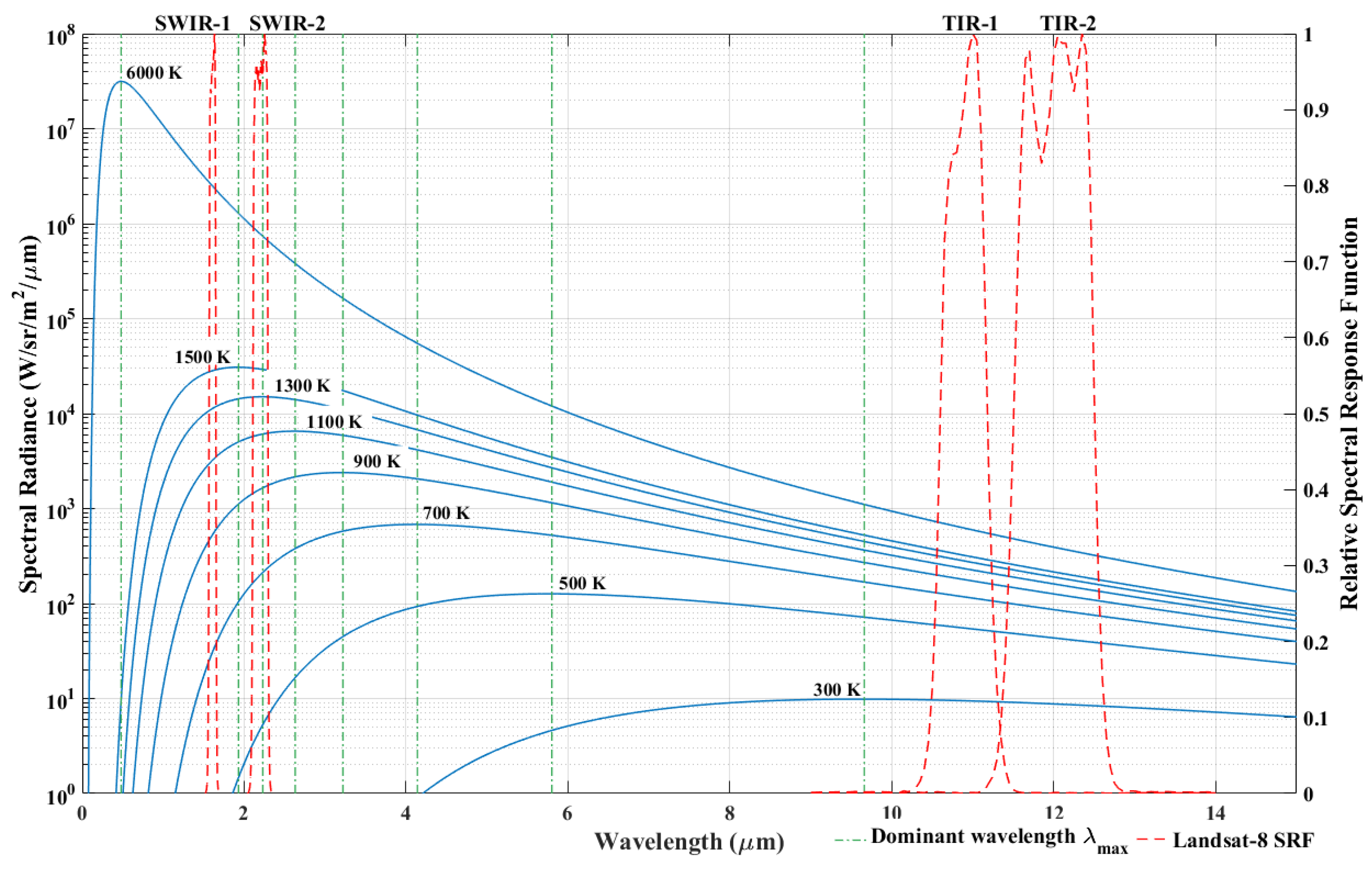
where A is Wien’s constant equal to , and is Stefan–Boltzmann constant equal to . Based on both theorems, as the temperature of a blackbody increases, the wavelength of peak radiance shifts to shorter wavelengths and the total emitted radiance from the blackbody increases as shown in Figure 1, and the shorter wavelength is more sensitive to higher temperatures. In terms of emitted radiation, Figure 1 shows that the maximum radiation at a temperature of 1300 K appears at a wavelength of 2.2 μm, which means that it is highly efficient in detecting wildfires, considering land surface temperatures range from 1000 K to 1500 K under flaming combustion [40], and the SWIR-2 spectral response function of the Landsat-8 OLI includes this wavelength. However, the detected radiance by the sensor is composed of reflected solar radiation and emitted thermal radiation. According to Murphy et al. [51], a single SWIR band has been frequently saturated at a 30-m spatial resolution, and this implied that the SWIR-2 band can be affected by land cover with a high spectral reflectance in that band. Despite the solar reflective effect, the SWIR-2 band could be input into the proposed method because the longer wavelength results in a reduction of solar reflective radiance. Giglio et al. [52] reported that the longest wavelength in the ASTER SWIR band (2.4 μm) could be selected as an input considering the flaming and smoldering response in the ratio of typical fire radiance to typical land surface radiance. Therefore, the SWIR-2 band was used to obtain high spatial resolution and high frequency temperature components in flaming combustion circumstances.
4.2. Proposed Disaggregation Method
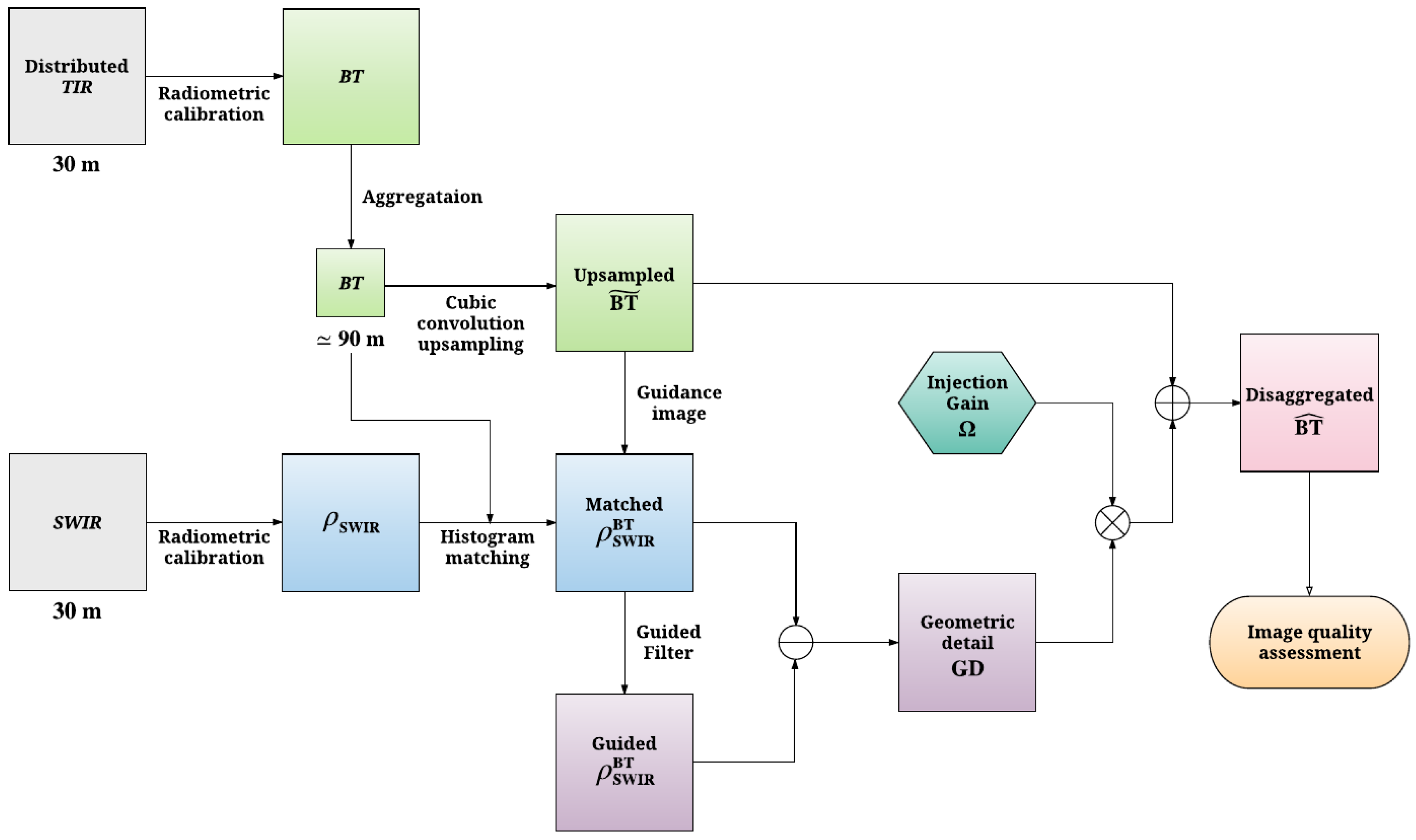
A flowchart of the proposed disaggregation method is described in Figure 2. Originally, the distributed Level 1 TIR data was already resampled to 30 m resolution by cubic convolution resampling [2]. To obtain the original resolution TIR image at 100 m resolution, an aggregation procedure was conducted on the Level 1 TIR data. However, the ratio between high- and low-resolution was rounded off to 3 because of effective image processing. The National Aeronautics and Space Administration has conducted a precise co-registration process for Landsat products [2]. Thus, the original resolution of the TIR dataset was assumed to be 90 m instead of 100 m. Also, the TIR-1 band data were selected because of the reported calibration issue. The main inputs of this method are only the TIR-1 band as brightness temperature (BT), and the SWIR-2 band as top-of-atmosphere (TOA) reflectance. After radiometric calibration, the BT imagery with 90-m resolution was upsampled at 30-m resolution, which is identical to that of SWIR imagery by cubic convolution resampling, and the upsampled BT imagery was used as guidance images for the GF. Histogram-matched SWIR imagery at 30-m resolution was selected for input images of the GF. High frequency components of BT could then be estimated as a result of GF. The difference between the TIR image and the approximation image from the GF can be considered as the GD from the TIR image. Injection gain was applied to the GD because of an energy matching issue. Finally, an injected GD of BT was merged with the original BT imagery.
4.2.1. Preprocessing
To obtain at-sensor spectral radiance, TOA reflectance, or at-sensor BT, the digital number (DN) must be converted using a radiometric calibration process [53]. First, the DN format of the image data was converted to an at-sensor spectral radiance () as follows:
where is a rescaling gain factor, is a rescaling offset factor, and are spectral at-sensor radiances that are scaled to and , respectively, and the unit of is . Based on the calculated at-sensor spectral radiance, TOA reflectance () and at-sensor BT () can be obtained by employing Equations (16) and (17):
where is earth-sun distance in astronomical units, is solar irradiance, is solar zenith angle, and , are calibration constants. In this study, the DN of VNIR and SWIR imagery were converted to TOA reflectance by using the fast line-of-sight atmospheric analysis of spectral hypercubes (FLAASH) model [54] which has been incorporated into the environment for visualizing images (ENVI) software. This allows for the DN of VNIR and SWIR images to be converted to TOA reflectance and that of TIR to be converted to BT. Converted TOA reflectance and BT were then used as an input of both the proposed and comparative thermal sharpening algorithms. The use of TOA reflectance reduced the effect of reflective solar radiance following the Earth-sun-satellite geometry [51].
4.2.2. Disaggregated Geometric Detail Using GF
After the radiometric calibration, the SWIR reflectance image () at 30-m resolution was histogram aligned with BT data (BT) from the TIR sensor at 90-m resolution to match the mean and standard deviation of the BT. Because of the inherent features of SWIR wavelengths, especially the SWIR-2 band in the Landsat-8 OLI sensor, the matched SWIR reflectance () was used to obtain high spatial resolution and a high frequency temperature component in flaming combustion circumstances instead of NDVI. In order to estimate the disaggregated GD (GD) of the BT image, the matched SWIR reflectance was selected as an input image of the GF, and the upsampled BT imagery was used as a guidance image of the GF. Therefore, the disaggregated GD of the BT was estimated by the GF because the guided SWIR () can preserve high frequency temperature components, as in flaming combustion conditions, with the variance tendency of the BT. The disaggregated GD of the BT was obtained by the difference of the histogram-matched SWIR and the guided SWIR in Equation (18):
where is histogram-matched SWIR reflectance imagery by the BT data, and is the upsampled BT. Thus, high frequency temperature components from SWIR images and structures of TIR images were preserved in the guided image, and the guided image could be used to obtain the disaggregated GD. Although the method of the disaggregation of thermal products influences the result of that method, the excessive or deficient window size also results in redundant information and produces artifacts in the resultant image [49]. In this study, the regularization parameter was set to 1, and performance with different window size was evaluated for the proposed method with quantitative image quality indices.
4.2.3. Injection Gain-Based on Data Statistics
The appropriate injection gain is an important factor for addition of GD information to the TIR image. The extraction of high frequency components and their effective injection are, generally, recognized as a single algorithm in an image fusion field [55]. If the injected spatial detail is not enough or is excessive, the spatial quality of the disaggregation image is not sufficient, or redundant information can lead to spectral distortion. In other words, in this study, the injection gain was considered as a process to reduce solar-reflected radiance in the SWIR-2 because the GD was obtained from the input of that band. Thus, this study strived to have the injection gain properly reflect the GD. Although the GD had a temperature component because the input of the GD was histogram-matched with the BT imagery, the distribution of the GD is highly skewed relative to the original BT imagery due to a high sensitivity of SWIR at the temperature of combustion. In order to achieve the proper energy matching between the GD and the BT imagery, injection gain was utilized in this study. The proposed injection gain is based on the ratio of the multiplication of the range and the skewness between the disaggregated GD and the original BT data as follows:
where is the injection gain proposed in this study, and are the range of the BT and the disaggregated GD, and and are the skewness of the BT and the disaggregated GD. Finally, considering the proposed injection gain, the disaggregation of the BT imagery can be described by Equation (20):
where is the disaggregated BT imagery at a 30 m resolution, and denotes a pixelwise multiplication operator.
4.3. Image Quality Assessment
To evaluate the quantitative image quality, five widely used quality indices were selected in this study. First, the root mean square error (RMSE) and the mean absolute error (MAE) are used to fundamentally evaluate the result of the image fusion process. The RMSE and MAE represent the difference and the bias between the fused image F and the reference image R. Both can be expressed by the following Equations (21) and (22):
where F(m,n) and R(m,n) represent the pixel values of the fused image, F, and the reference image R, at the mth column and nth row, and M × N is the size of the reference image. Lower values for RMSE and MAE indicate a lower error for the fused image. Second, the correlation coefficient (CC) is also used to assess the fused images. The CC of a fused image and its reference image reflects the similarity of spectral information. The formulation is Equation (23) as follows:
where and are the mean of the fused image and the reference image, respectively. If the two images are correlated, the CC is close to 1, which implies that the spectral features of the original image were preserved well during the disaggregation process. Also, the image quality Q index, also known as the universal image quality index (UIQI), reflects the structural distortion degree [56]. UIQI is defined in Equation (24) as follows:
where is the covariance matrix between the fused image and the reference image, and and are the standard deviations of the fused image and the reference image. The UIQI was applied to the disaggregated results with an 8 × 8 distinct window. If its value is close to 1, the quality of the fused image is adequate. Finally, erreur relative globale adimensionelle de synthèse (ERGAS) is useful to evaluate the overall quality of the disaggregated image [3]. It represents the degree to which the disaggregated image and the reference image are different. The ERGAS is defined in Equation (25) as follows:
where is the scale ratio between the pixel sizes of the SWIR image and the BT image, is the RMSE between the ith fused band and the reference band, and is the mean of the ith reference band. Thus, a small value of ERGAS means a small spectral distortion is present in the disaggregated image.
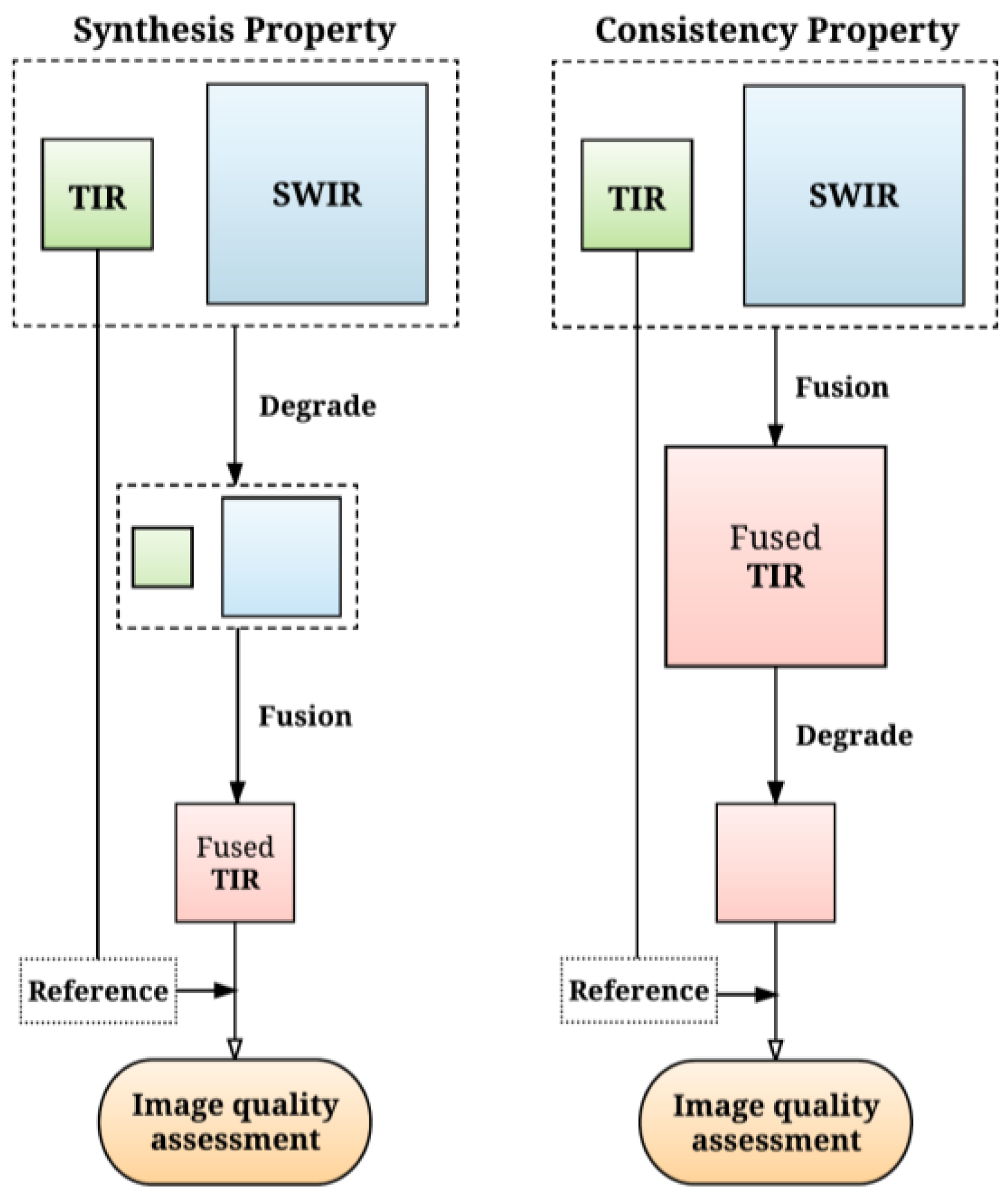
There are two validation methods that are commonly used to assess the quality of the fused image. The first is the synthesis property, and the other is the consistency property as shown in Figure 3. First, the synthesis property considers that the disaggregated image should be as close to identical to the acquired input image as possible. However, at the full-resolution scale, assessment of the synthesis property is not possible, thus the fusion images, SWIR and TIR, were degraded by the scale ratio between the pixel sizes of the SWIR image and the BT image. The degraded images were used as an input of the disaggregation method, and the degraded fused image was compared to the original observed BT image as a reference. Second, the consistency property reflects the degree to which the spatially degraded fused image is identical to the original observed BT image. Cubic convolution interpolation was applied for image degradation of the synthesis and consistency properties. To validate the evaluation process, both synthesis and the consistency properties were applied to our experimental assessments.
5. Experimental Results
5.1. Study Area
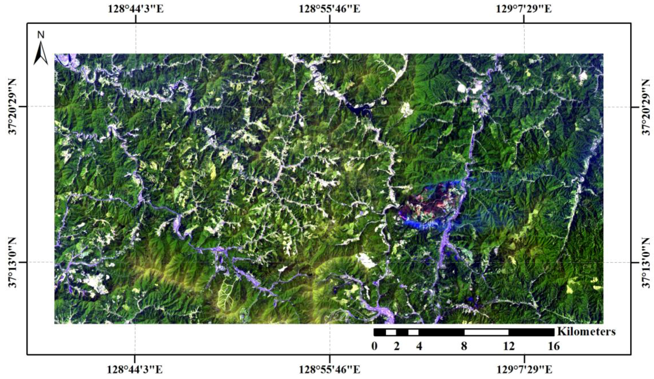
On 6 May 2017, a series of wildfires that destroyed more than thirty homes and caused the evacuation of 2500 residents occurred simultaneously in Samcheok, Gangneung and Sangju, cities in South Korea. Together, these fires burned nearly 150 ha. Especially dry climate conditions in spring promoted the rapid growth of the wildfires. The study area is located in Samcheok city, Gangwon province, one of the areas affected by the spring 2017 fires (Figure 4). For the proposed thermal disaggregation and comparative processes, freely accessible Landsat-8 Level-1 OLI and TIRS datasets, with a spatial resolution of 30 m in the VNIR and SWIR bands and 30 m in the TIR bands (originally, 100 m), were acquired from the USGS Earth Explorer website [57]. The datasets were acquired at 01:58:02 GMT (10:58:02 local time), May 8th, 2017 from the 114 path and 34 row in the world reference system-2 (WRS-2). The acquisition datasets were clipped including the wildfires and marginal cloud-free areas, and the size of the TIR images was 267 × 543 pixels, and that of the MS images was 801 × 1629 pixels. Considering the two-day gap between the initiated wildfire and the image acquisition date, the datasets are expected to include a variety of wildfire components, for example, flaming combustion, smoldering combustion, and burned areas. In particular, flaming combustion, a core of wildfires, is remarkably shown in the acquired imagery (refer to Figure 4).
5.2. Analysis of the Disaggregation Methods
Experiments were conducted to evaluate the performance of the proposed disaggregation of TIR imagery using Landsat-8 datasets. The proposed algorithm was compared with DisTrad [6], TsHARP [7], and the LMS method [12]. Evaluation of the disaggregation methods focused on the synthesis and consistency properties [55]. The reflectance of the SWIR-2 band from the Landsat-8 OLI sensor was selected as the input of the proposed algorithm, and the GF filter constrained the input imagery by using the guidance image, and original TIR data at a coarser resolution. The results of the proposed disaggregation algorithm and the comparison disaggregation methods were considered, and the disaggregated image quality assessment was then conducted with parameter configuration (window size) of the GF.
5.2.1. Visual Analysis
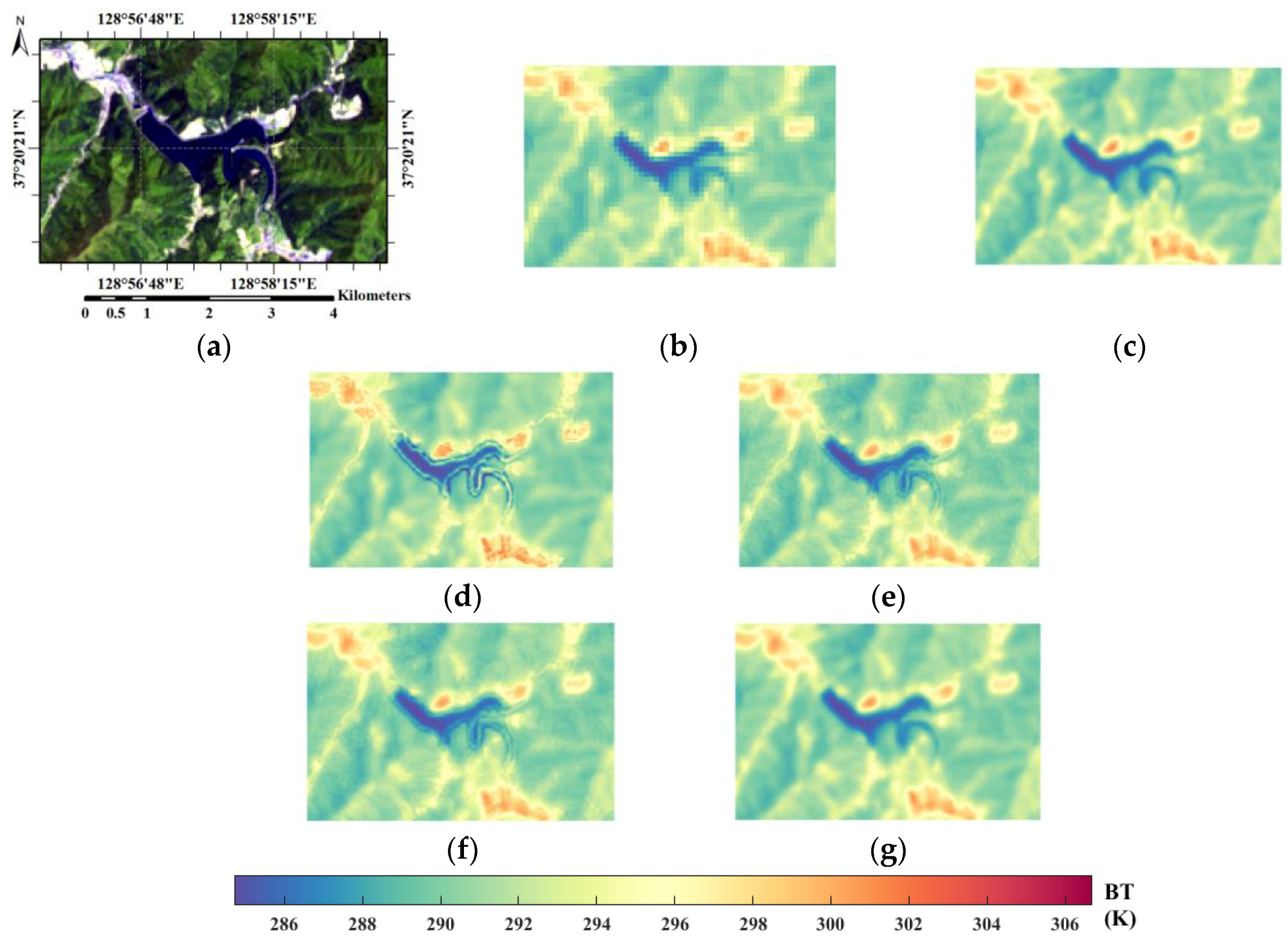
The proposed disaggregation method was compared with the DisTrad, TsHARP, and the LMS methods. Figure 5 shows the result of the disaggregated BT image obtained using the proposed SWIR and the GF-based algorithm with the color composite image, the original BT image at a resolution of 90 m, and the distributed BT image from Earth Explorer at a 30 m resolution. To qualitatively evaluate the results, three subsets of the disaggregated images, A, B, and C in Figure 5 were obtained, and comparison with VI-based methods including DisTrad, TsHARP, and LMS was conducted directly in the selected subset areas as shown in Figure 6, Figure 7 and Figure 8. There were two notable features of the results from the proposed method in terms of qualitative analysis. First, the proposed algorithm performed well on wildfire areas, spatially preserving high frequency temperature components (Figure 6 and Figure 7). The comparison algorithms had lower BT values in the disaggregated image on burning areas, but the proposed algorithm produced higher BT values on the same burning areas. Also, removal of ringing artifacts was demonstrated in the disaggregated image of our proposed algorithm. Figure 8 shows the subset of the disaggregated images near the lake. The ringing artefacts near the lake edge were eliminated by the proposed algorithm but appear in the results of other algorithms (Figure 8). As shown in the visual evaluation, this experiment confirmed that the proposed algorithm can provide visually satisfactory results with regard to the original BT image.
5.2.2. Quantitative Analysis
Table 1 presents the results of quantitative analyses depending on different window size. As shown in Table 1, the best performance of the proposed method was obtained from window size 5 × 5 of the GF. The units of RMSE and MAE are Kelvin in this study. The results of the disaggregated image quality assessment based on the synthesis property are presented in Table 2.
The disaggregated image obtained by the DisTrad algorithm indicates that all quality indices had poor results, but the TsHARP algorithm, a refined version of the DisTrad, shows better results in comparison with the DisTrad. The disaggregation result of the LMS algorithm was similar to that of the TsHARP algorithm. Finally, the results of the proposed algorithm, indicated by GF, have the best values of RMSE, MAE, CC, UIQI and ERGAS compared to other algorithms. The thermal variance of the original BT data was therefore preserved in the disaggregated result for the proposed GF algorithm. For the consistency property, the results of quantitative analysis also show similar trends compared to the synthesis property, and here the proposed GF algorithm provides the best quality indices results for all consistency properties (Table 2).
6. Discussion
In this study, disaggregation of BT imagery of Landsat-8 from 90-m resolution to 30-m resolution on wildfire areas was conducted by using the guided SWIR-2 band of Landsat-8 OLI. The experimental results showed that the comparison methods were limited on wildfire areas, but the proposed algorithm yielded better disaggregated BT images in terms of qualitative and quantitative analysis. In particular, the qualitative evaluation of the experimental results demonstrated that the high temperature component from SWIR was preserved in the guided filtering process on the burning areas, and the SWIR band as the input of disaggregation process supplemented the limitation of TIR sensor of restricted detection of high temperature in active fires. Also, most previous disaggregation studies improved spatial detail from the MS band products, but did not consider the thermal variation of the TIR data. This occurrence of spectral distortion in the disaggregation process results because of an injection effect of redundant detail. In contrast, the thermal variation of the original BT image was preserved simultaneously with improved spatial resolution of the BT by the GF, using the original BT data as a guidance image as described in the quantitative analysis discussion (Section 5.2.2).
In the study area, there are two main wildfire components, flaming and smoldering. Despite the mixed-pixel problem within the wildfire component and unburned fuel component, Yu et al. [58] reported that the critical fraction of recognition was 1/500 of the 30-m resolution cell on an experimental hotspot target (955 K) in the Landsat SWIR band, and Giglio et al. [52] suggested that the TIR band (8.3 μm) of the ASTER data would be the best choice for detecting smoldering considering the solar reflective effect. As a result, for a flaming combustion region, the disaggregated BT was relatively higher in the margin area in the proposed disaggregation method due to the input of the SWIR-2 band, and the smoldering effect was also reflected by the tendency of the TIR band. However, temperature of the combustion region is not equal to the disaggregated BT due to a land surface temperature range from 1000 K to 1500 K in flaming combustion conditions [40]. Also, conversion the BT into land surface temperature was not conducted in this work. Although these limitations existed in this study, the application of the proposed disaggregation algorithm was proved valuable for middle-high spatial resolution imagery using Landsat-8 products, considering the limited Landsat-8 data availability on the active fire areas.
Despite applications of the TOA reflectance as an input and injection gain, the disaggregation results could hardly be free from reflective solar radiation for daytime analysis. Manmade land cover (e.g., concrete, rooftops, and highly reflective paint) and arid soil area especially have high reflectance in the SWIR-2 band. The proposed algorithm additionally used the TIR imagery, which is insensitive to reflected solar radiation [59], during the process of GF filtering. In this case, the TIR imagery was used as a guidance image and compensated for the high frequency components from the high solar reflectance. Also, the effect of reflective solar radiation depends on the characteristics of the experimental area. The study area is a typically rural and mountainous area with a low population density. In terms of disaggregation, manmade land cover could be a high frequency temperature component during the daytime because the temperature of manmade structures is higher than that of vegetation, and the high solar reflectance reflected the tendency of the BT in the experimental areas. Only for a high solar reflectance near the flaming case could the high temperature term be extended near the flaming area. However, the thermally emitted radiation must be distinct from the solar-reflected radiation in the case of an arid or urban area. To avoid a saturation problem, an alternative daytime hot spot detection algorithm was suggested using separate wavebands including NIR, SWIR-1, and SWIR-2 of the Landsat datasets [51]. Therefore, additive band datasets, the NIR and the shorter SWIR band, will be considered in a future work to reduce the effect of solar reflectance and potential saturation in the SWIR-2 band.
This study expected to apply the proposed algorithm to improve the spatial resolution without spectral distortion in the production of Landsat thermal images Application of the proposed method can be extended to geostationary products that have low spatial and high temporal resolutions, for example, moderate resolution imaging spectroradiometer (MODIS) and visual infrared imaging radiometer suite (VIIRS) which cover the SWIR and TIR bands with diurnal temporal resolution. Consequently, data fusion with the advantages of high temporal geostationary products and high spatial resolution, termed spatial-temporal disaggregation, can be conducted using the proposed method based on the GF. Future work will be focused on the application of the proposed disaggregation algorithm to improve the spatial-temporal resolution of the TIR data.
7. Conclusions
In this study, the efficient and improved disaggregation algorithm of TIR imagery using guided SWIR imagery was proposed for wildfire conditions. The SWIR imagery radiometrically satisfied the preservation of a high temperature component in flaming combustion, and the GF prevented the spectral distortion of the original TIR data and simultaneously preserved the high frequency component of SWIR image in the disaggregated result. Landsat-8 OLI and TIRS images, captured at the wildfire site, were used to evaluate the proposed algorithm with the existing disaggregation algorithms based on VI originated from VNIR. The experimental results demonstrated that the proposed algorithm disaggregated the BT data from 90-m resolution to 30-m resolution and satisfied image quality assessments in terms of visual and quantitative evaluation. In the quantitative evaluation, RMSE, MAE, CC, ERGAS, and UIQI had better results (Table 2) in the proposed algorithm than those of the other comparison methods. Also, visual analysis (Figure 6 and Figure 7) demonstrated that the proposed algorithm conducted the disaggregation of the TIR imagery reflecting the temperature of wildfire areas. The experimental results show that the proposed algorithm was successfully applied to Landsat-8 OLI and TIRS datasets from wildfire areas. In future work, the proposed method will be developed considering the effect of SWIR saturation, and also applied to spatio-temporal disaggregation with a geostationary image and Landsat datasets.
Acknowledgments
This research was supported by the Nation Research Foundation of Korea under Grant NRF-2015M1A3A3A02014673.
Author Contribution
Kangjoon Cho conceived and designed the experiments and prepared the manuscript; Yonghyun Kim performed the experiments and contributed analysis tools; Yongil Kim offered invaluable suggestions for the design of the experiments and directed the research.
Conflicts of Interest
The authors declare no conflict of interest.
References
- Kalma, J.D.; McVicar, T.R.; McCabe, M.F. Estimating land surface evaporation: A review of methods using remotely sensed surface temperature data. Surv. Geophys. 2008, 29, 421–469. [Google Scholar] [CrossRef]
- Roy, D.P.; Wulder, M.; Loveland, T.R.; Woodcock, C.; Allen, R.; Anderson, M.; Helder, D.; Irons, J.; Johnson, D.; Kennedy, R. Landsat-8: Science and product vision for terrestrial global change research. Remote Sens. Environ. 2014, 145, 154–172. [Google Scholar] [CrossRef]
- Zhan, W.; Chen, Y.; Zhou, J.; Li, J.; Liu, W. Sharpening thermal imageries: A generalized theoretical framework from an assimilation perspective. IEEE Trans. Geosci. Remote Sens. 2011, 49, 773–789. [Google Scholar] [CrossRef]
- Chen, Y.; Zhan, W.; Quan, J.; Zhou, J.; Zhu, X.; Sun, H. Disaggregation of remotely sensed land surface temperature: A generalized paradigm. IEEE Trans. Geosci. Remote Sens. 2014, 52, 5952–5965. [Google Scholar] [CrossRef]
- Zhan, W.; Chen, Y.; Zhou, J.; Wang, J.; Liu, W.; Voogt, J.; Zhu, X.; Quan, J.; Li, J. Disaggregation of remotely sensed land surface temperature: Literature survey, taxonomy, issues, and caveats. Remote Sens. Environ. 2013, 131, 119–139. [Google Scholar] [CrossRef]
- Kustas, W.P.; Norman, J.M.; Anderson, M.C.; French, A.N. Estimating subpixel surface temperatures and energy fluxes from the vegetation index-radiometric temperature relationship. Remote Sens. Environ. 2003, 85, 429–440. [Google Scholar] [CrossRef]
- Agam, N.; Kustas, W.P.; Anderson, M.C.; Li, F.; Neale, C.M. A vegetation index based technique for spatial sharpening of thermal imagery. Remote Sens. Environ. 2007, 107, 545–558. [Google Scholar] [CrossRef]
- Guo, L.J.; Moore, J.M. Pixel block intensity modulation: Adding spatial detail to TM band 6 thermal imagery. Int. J. Remote Sens. 1998, 19, 2477–2491. [Google Scholar] [CrossRef]
- Stathopoulou, M.; Cartalis, C. Downscaling AVHRR land surface temperatures for improved surface urban heat island intensity estimation. Remote Sens. Environ. 2009, 113, 2592–2605. [Google Scholar] [CrossRef]
- Dominguez, A.; Kleissl, J.; Luvall, J.C.; Rickman, D.L. High-resolution urban thermal sharpener (HUTS). Remote Sens. Environ. 2011, 115, 1772–1780. [Google Scholar] [CrossRef]
- Jeganathan, C.; Hamm, N.; Mukherjee, S.; Atkinson, P.M.; Raju, P.; Dadhwal, V. Evaluating a thermal image sharpening model over a mixed agricultural landscape in India. Int. J. Appl. Earth Obs. Geoinf. 2011, 13, 178–191. [Google Scholar] [CrossRef]
- Mukherjee, S.; Joshi, P.; Garg, R. A comparison of different regression models for downscaling Landsat and MODIS land surface temperature images over heterogeneous landscape. Adv. Space Res. 2014, 54, 655–669. [Google Scholar] [CrossRef]
- Bisquert, M.; Sánchez, J.M.; Caselles, V. Evaluation of disaggregation methods for downscaling MODIS land surface temperature to Landsat spatial resolution in Barrax test site. IEEE J. Sel. Top. Appl. Earth Obs. Remote Sens. 2016, 9, 1430–1438. [Google Scholar] [CrossRef]
- Gao, L.; Zhan, W.; Huang, F.; Quan, J.; Lu, X.; Wang, F.; Ju, W.; Zhou, J. Localization or Globalization? Determination of the Optimal Regression Window for Disaggregation of Land Surface Temperature. IEEE Trans. Geosci. Remote Sens. 2017, 55, 477–490. [Google Scholar] [CrossRef]
- Mukherjee, S.; Joshi, P.; Garg, R. Analysis of urban built-up areas and surface urban heat island using downscaled MODIS derived land surface temperature data. Geocarto Int. 2017, 32, 900–918. [Google Scholar] [CrossRef]
- Merlin, O.; Duchemin, B.; Hagolle, O.; Jacob, F.; Coudert, B.; Chehbouni, G.; Dedieu, G.; Garatuza, J.; Kerr, Y. Disaggregation of MODIS surface temperature over an agricultural area using a time series of Formosat-2 images. Remote Sens. Environ. 2010, 114, 2500–2512. [Google Scholar] [CrossRef] [Green Version]
- Li, J.; Song, C.; Cao, L.; Zhu, F.; Meng, X.; Wu, J. Impacts of landscape structure on surface urban heat islands: A case study of Shanghai, China. Remote Sens. Environ. 2011, 115, 3249–3263. [Google Scholar] [CrossRef]
- Yang, H.; Cong, Z.; Liu, Z.; Lei, Z. Estimating sub-pixel temperatures using the triangle algorithm. Int. J. Remote Sens. 2010, 31, 6047–6060. [Google Scholar] [CrossRef]
- Essa, W.; Verbeiren, B.; van der Kwast, J.; Van de Voorde, T.; Batelaan, O. Evaluation of the DisTrad thermal sharpening methodology for urban areas. Int. J. Appl. Earth Obs. Geoinf. 2012, 19, 163–172. [Google Scholar] [CrossRef]
- Bindhu, V.; Narasimhan, B.; Sudheer, K. Development and verification of a non-linear disaggregation method (NL-DisTrad) to downscale MODIS land surface temperature to the spatial scale of Landsat thermal data to estimate evapotranspiration. Remote Sens. Environ. 2013, 135, 118–129. [Google Scholar] [CrossRef]
- Kolios, S.; Georgoulas, G.; Stylios, C. Achieving downscaling of Meteosat thermal infrared imagery using artificial neural networks. Int. J. Remote Sens. 2013, 34, 7706–7722. [Google Scholar] [CrossRef]
- Yang, G.; Pu, R.; Zhao, C.; Huang, W.; Wang, J. Estimation of subpixel land surface temperature using an endmember index based technique: A case examination on ASTER and MODIS temperature products over a heterogeneous area. Remote Sens. Environ. 2011, 115, 1202–1219. [Google Scholar] [CrossRef]
- Chen, X.; Li, W.; Chen, J.; Rao, Y.; Yamaguchi, Y. A combination of TsHARP and thin plate spline interpolation for spatial sharpening of thermal imagery. Remote Sens. 2014, 6, 2845–2863. [Google Scholar] [CrossRef]
- Rodriguez-Galiano, V.; Pardo-Igúzquiza, E.; Sanchez-Castillo, M.; Chica-Olmo, M.; Chica-Rivas, M. Downscaling Landsat 7 ETM+ thermal imagery using land surface temperature and NDVI images. Int. J. Appl. Earth Obs. Geoinf. 2012, 18, 515–527. [Google Scholar] [CrossRef]
- Moosavi, V.; Talebi, A.; Mokhtari, M.H.; Shamsi, S.R.F.; Niazi, Y. A wavelet-artificial intelligence fusion approach (WAIFA) for blending Landsat and MODIS surface temperature. Remote Sens. Environ. 2015, 169, 243–254. [Google Scholar] [CrossRef]
- Hutengs, C.; Vohland, M. Downscaling land surface temperatures at regional scales with random forest regression. Remote Sens. Environ. 2016, 178, 127–141. [Google Scholar] [CrossRef]
- Yang, Y.; Cao, C.; Pan, X.; Li, X.; Zhu, X. Downscaling Land Surface Temperature in an Arid Area by Using Multiple Remote Sensing Indices with Random Forest Regression. Remote Sens. 2017, 9, 789. [Google Scholar] [CrossRef]
- Sismanidis, P.; Keramitsoglou, I.; Bechtel, B.; Kiranoudis, C.T. Improving the downscaling of diurnal land surface temperatures using the annual cycle parameters as disaggregation kernels. Remote Sens. 2017, 9, 23. [Google Scholar] [CrossRef]
- Sismanidis, P.; Keramitsoglou, I.; Kiranoudis, C.T.; Bechtel, B. Assessing the capability of a downscaled urban land surface temperature time series to reproduce the spatiotemporal features of the original data. Remote Sens. 2016, 8, 274. [Google Scholar] [CrossRef]
- Zhan, W.; Huang, F.; Quan, J.; Zhu, X.; Gao, L.; Zhou, J.; Ju, W. Disaggregation of remotely sensed land surface temperature: A new dynamic methodology. J. Geophys. Res. Atmos. 2016, 121, 10538–10554. [Google Scholar] [CrossRef]
- Jia, Y.; Huang, Y.; Yu, B.; Wu, Q.; Yu, S.; Wu, J.; Wu, J. Downscaling land surface temperature data by fusing Suomi NPP-VIIRS and landsat-8 TIR data. Remote Sens. Lett. 2017, 8, 1133–1142. [Google Scholar]
- Bisquert, M.; Sánchez, J.; López-Urrea, R.; Caselles, V. Estimating high resolution evapotranspiration from disaggregated thermal images. Remote Sens. Environ. 2016, 187, 423–433. [Google Scholar] [CrossRef]
- Singh, R.K.; Senay, G.B.; Velpuri, N.M.; Bohms, S.; Verdin, J.P. On the downscaling of actual evapotranspiration maps based on combination of MODIS and Landsat-based actual evapotranspiration estimates. Remote Sens. 2014, 6, 10483–10509. [Google Scholar] [CrossRef]
- Olivera-Guerra, L.; Mattar, C.; Merlin, O.; Durán-Alarcón, C.; Santamaría-Artigas, A.; Fuster, R. An operational method for the disaggregation of land surface temperature to estimate actual evapotranspiration in the arid region of Chile. ISPRS J. Photogramm. Remote Sens. 2017, 128, 170–181. [Google Scholar] [CrossRef]
- Jiang, Y.; Weng, Q. Estimation of hourly and daily evapotranspiration and soil moisture using downscaled LST over various urban surfaces. GISci. Remote Sens. 2017, 54, 95–117. [Google Scholar] [CrossRef]
- Nichol, J. An emissivity modulation method for spatial enhancement of thermal satellite images in urban heat island analysis. Photogramm. Eng. Remote Sens. 2009, 75, 547–556. [Google Scholar] [CrossRef]
- Zakšek, K.; Oštir, K. Downscaling land surface temperature for urban heat island diurnal cycle analysis. Remote Sens. Environ. 2012, 117, 114–124. [Google Scholar] [CrossRef]
- Li, X.; Xin, X.; Jiao, J.; Peng, Z.; Zhang, H.; Shao, S.; Liu, Q. Estimating Subpixel Surface Heat Fluxes through Applying Temperature-Sharpening Methods to MODIS Data. Remote Sens. 2017, 9, 836. [Google Scholar] [CrossRef]
- Zhang, D.; Tang, R.; Zhao, W.; Tang, B.; Wu, H.; Shao, K.; Li, Z.-L. Surface soil water content estimation from thermal remote sensing based on the temporal variation of land surface temperature. Remote Sens. 2014, 6, 3170–3187. [Google Scholar] [CrossRef] [Green Version]
- Dennison, P.E.; Charoensiri, K.; Roberts, D.A.; Peterson, S.H.; Green, R.O. Wildfire temperature and land cover modeling using hyperspectral data. Remote Sens. Environ. 2006, 100, 212–222. [Google Scholar] [CrossRef]
- Schroeder, T.A.; Wulder, M.A.; Healey, S.P.; Moisen, G.G. Mapping wildfire and clearcut harvest disturbances in boreal forests with Landsat time series data. Remote Sens. Environ. 2011, 115, 1421–1433. [Google Scholar] [CrossRef]
- Allison, R.S.; Johnston, J.M.; Craig, G.; Jennings, S. Airborne optical and thermal remote sensing for wildfire detection and monitoring. Sensors 2016, 16, 1310. [Google Scholar] [CrossRef] [PubMed]
- Blackett, M. Early analysis of Landsat-8 thermal infrared sensor imagery of volcanic activity. Remote Sens. 2014, 6, 2282–2295. [Google Scholar] [CrossRef]
- Zakšek, K.; Hort, M.; Lorenz, E. Satellite and ground based thermal observation of the 2014 effusive eruption at Stromboli volcano. Remote Sens. 2015, 7, 17190–17211. [Google Scholar] [CrossRef]
- Sun, L.; Schulz, K. The improvement of land cover classification by thermal remote sensing. Remote Sens. 2015, 7, 8368–8390. [Google Scholar] [CrossRef]
- Bonafoni, S. Downscaling of Landsat and MODIS land surface temperature over the heterogeneous urban area of Milan. IEEE J. Sel. Top. Appl. Earth Obs. Remote Sens. 2016, 9, 2019–2027. [Google Scholar] [CrossRef]
- He, K.; Sun, J.; Tang, X. Guided image filtering. IEEE Trans. Pattern Anal. Mach. Intell. 2013, 35, 1397–1409. [Google Scholar] [CrossRef] [PubMed]
- Liu, J.; Liang, S. Pan-sharpening using a guided filter. Int. J. Remote Sens. 2016, 37, 1777–1800. [Google Scholar] [CrossRef]
- Yang, Y.; Wan, W.; Huang, S.; Yuan, F.; Yang, S.; Que, Y. Remote sensing image fusion based on adaptive IHS and multiscale guided filter. IEEE Access 2016, 4, 4573–4582. [Google Scholar] [CrossRef]
- Upla, K.P.; Joshi, S.; Joshi, M.V.; Gajjar, P.P. Multiresolution image fusion using edge-preserving filters. J. Appl. Remote Sens. 2015, 9, 1–26. [Google Scholar] [CrossRef]
- Murphy, S.W.; de Souza Filho, C.R.; Wright, R.; Sabatino, G.; Pabon, R.C. HOTMAP: Global hot target detection at moderate spatial resolution. Remote Sens. Environ. 2016, 177, 78–88. [Google Scholar] [CrossRef]
- Giglio, L.; Csiszar, I.; Restás, Á.; Morisette, J.T.; Schroeder, W.; Morton, D.; Justice, C.O. Active fire detection and characterization with the advanced spaceborne thermal emission and reflection radiometer (ASTER). Remote Sens. Environ. 2008, 112, 3055–3063. [Google Scholar] [CrossRef]
- Chander, G.; Markham, B.L.; Helder, D.L. Summary of current radiometric calibration coefficients for Landsat MSS, TM, ETM+, and EO-1 ALI sensors. Remote Sens. Environ. 2009, 113, 893–903. [Google Scholar] [CrossRef]
- Felde, G.; Anderson, G.; Cooley, T.; Matthew, M.; Berk, A.; Lee, J. Analysis of Hyperion data with the FLAASH atmospheric correction algorithm. In Proceedings of the 2003 IEEE International Geoscience and Remote Sensing Symposium, Toulouse, France, 21–25 July 2003; pp. 90–92. [Google Scholar]
- Vivone, G.; Alparone, L.; Chanussot, J.; Dalla Mura, M.; Garzelli, A.; Licciardi, G.A.; Restaino, R.; Wald, L. A critical comparison among pansharpening algorithms. IEEE Trans. Geosci. Remote Sens. 2015, 53, 2565–2586. [Google Scholar] [CrossRef]
- Wang, Z.; Bovik, A.C. A universal image qulity index. IEEE Signal Pocess. Lett. 2002, 9, 81–84. [Google Scholar] [CrossRef]
- United States Geological Survey. USGS Earth Explorer. 2017. Available online: http://earthexplorer.usgs.gov (accessed on 11 December 2017).
- Yu, Y.; Xing, L.; Pan, J.; Jiang, L.; Yu, H. Study of high temperature targets identification and temperature retrieval experimental model in SWIR remote sensing based Landsat8. Int. J. Appl. Earth Obs. Geoinf. 2016, 46, 56–62. [Google Scholar] [CrossRef]
- Morisette, J.T.; Giglio, L.; Csiszar, I.; Justice, C.O. Validation of the MODIS active fire product over Southern Africa with ASTER data. Int. J. Remote Sens. 2005, 26, 4239–4264. [Google Scholar] [CrossRef]
Figure 1.
Blackbody radiation curves at different blackbody temperatures, as derived from Plank’s law, and relative spectral response functions of the Landsat-8 operational land imager (OLI) and thermal infrared sensor (TIRS).
Figure 1.
Blackbody radiation curves at different blackbody temperatures, as derived from Plank’s law, and relative spectral response functions of the Landsat-8 operational land imager (OLI) and thermal infrared sensor (TIRS).

Figure 2.
Flowchart for the proposed disaggregation method of TIR data.

Figure 3.
Overview of synthesis and consistency properties for evaluation of disaggregated image quality.
Figure 3.
Overview of synthesis and consistency properties for evaluation of disaggregated image quality.

Figure 4.
SWIR2-SWIR1-Blue color composites of the study area affected by wildfires.

Figure 5.
Proposed disaggregated brightness temperature results.
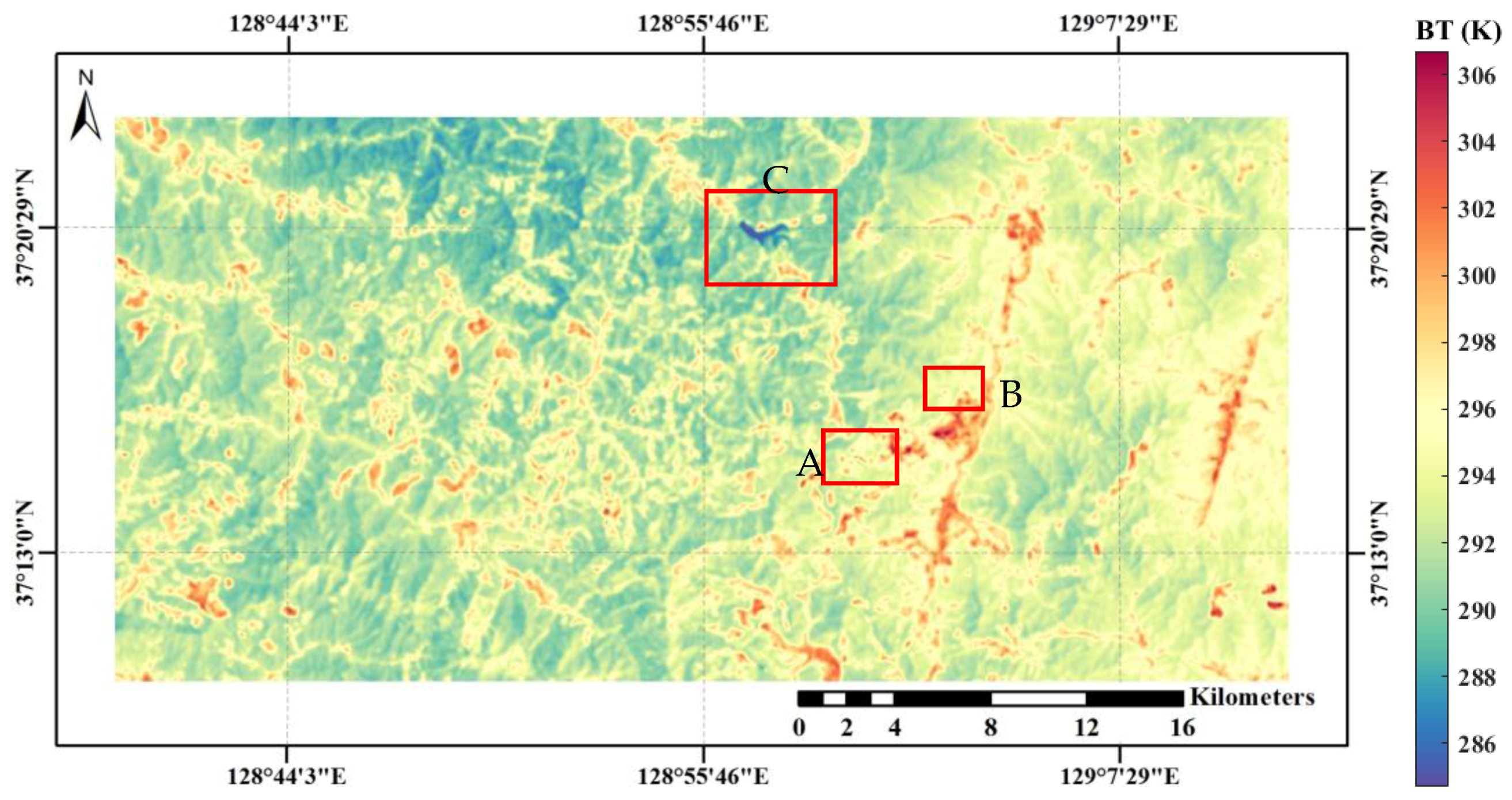
Figure 6.
Disaggregated brightness temperature results at subset A: (a) SWIR2-SWIR1-Blue composite image; (b) Original BT image; (c) Distributed BT image; (d) DisTrad method; (e) TsHARP method; (f) LMS method; (g) Proposed GF method.
Figure 6.
Disaggregated brightness temperature results at subset A: (a) SWIR2-SWIR1-Blue composite image; (b) Original BT image; (c) Distributed BT image; (d) DisTrad method; (e) TsHARP method; (f) LMS method; (g) Proposed GF method.
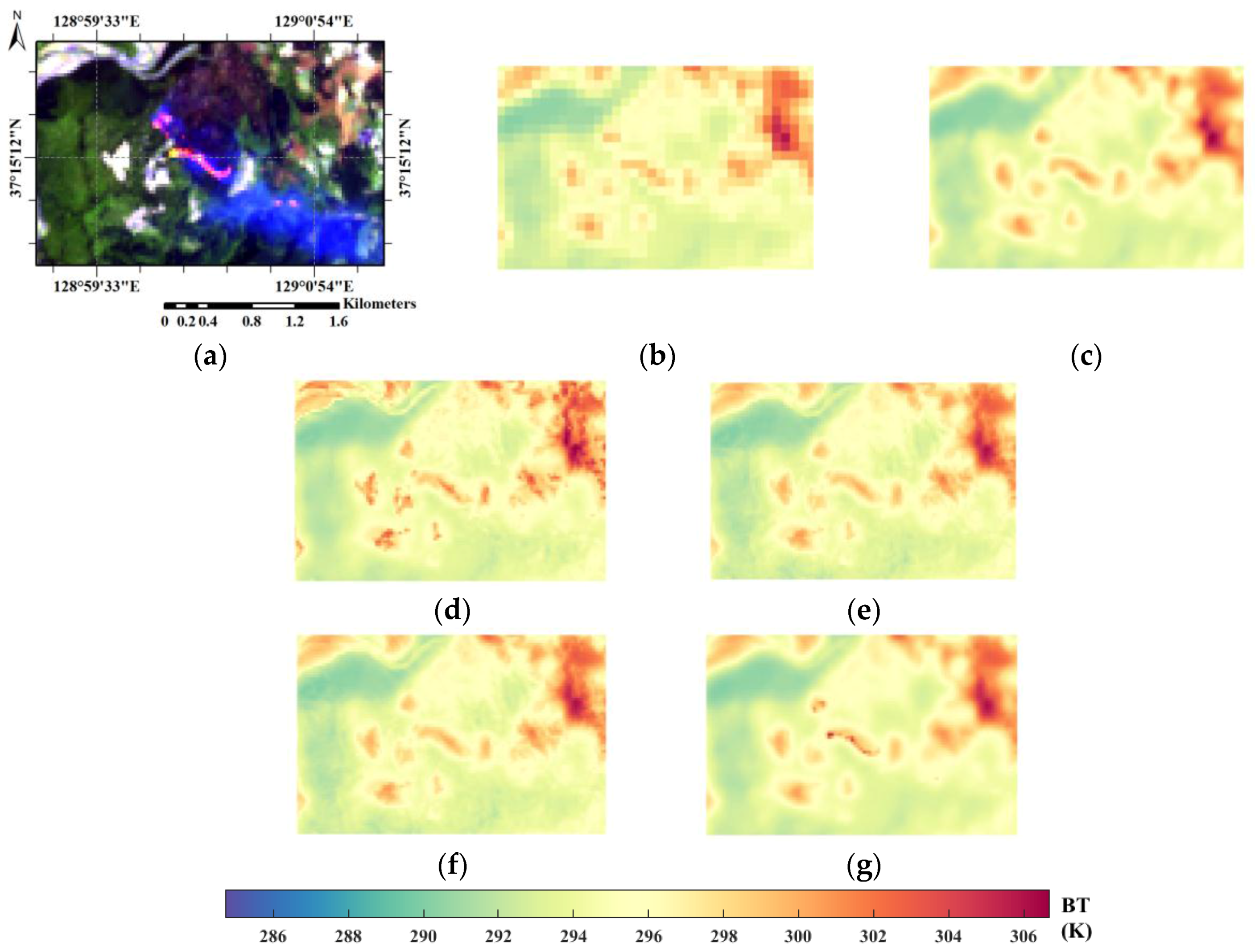
Figure 7.
Disaggregated brightness temperature results at subset B: (a) SWIR2-SWIR1-Blue composite image; (b) Original BT image; (c) Distributed BT image; (d) DisTrad method; (e) TsHARP method; (f) LMS method; (g) Proposed GF method.
Figure 7.
Disaggregated brightness temperature results at subset B: (a) SWIR2-SWIR1-Blue composite image; (b) Original BT image; (c) Distributed BT image; (d) DisTrad method; (e) TsHARP method; (f) LMS method; (g) Proposed GF method.
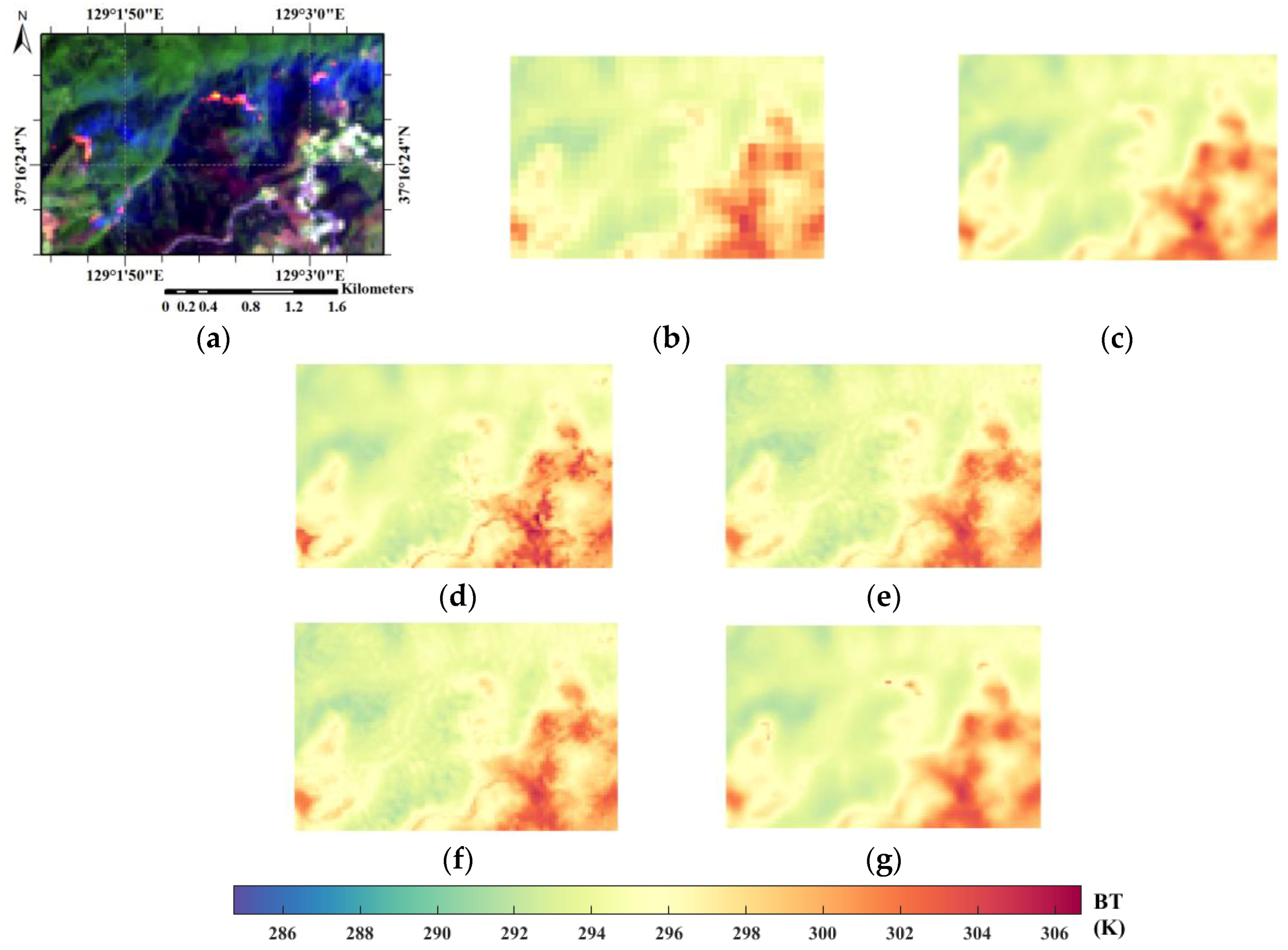
Figure 8.
Disaggregated brightness temperature results at subset C: (a) SWIR2-SWIR1-Blue composite image; (b) Original BT image; (c) Distributed BT image; (d) DisTrad method; (e) TsHARP method; (f) LMS method; (g) Proposed GF method.
Figure 8.
Disaggregated brightness temperature results at subset C: (a) SWIR2-SWIR1-Blue composite image; (b) Original BT image; (c) Distributed BT image; (d) DisTrad method; (e) TsHARP method; (f) LMS method; (g) Proposed GF method.

Table 1.
Quantitative evaluation of the proposed method depending on different window size. The optimal values in terms of quality index are highlighted in bold.
Table 1.
Quantitative evaluation of the proposed method depending on different window size. The optimal values in terms of quality index are highlighted in bold.
| Window Size | ||||||||||
|---|---|---|---|---|---|---|---|---|---|---|
| 3 × 3 | 5 × 5 | 7 × 7 | 9 × 9 | 11 × 11 | 13 × 13 | 15 × 15 | 17 × 17 | 19 × 19 | ||
| RMSE | 0.073 | 0.072 | 0.073 | 0.074 | 0.074 | 0.075 | 0.076 | 0.076 | 0.077 | |
| CC | 0.9996 | 0.9996 | 0.9996 | 0.9996 | 0.9996 | 0.9996 | 0.9995 | 0.9995 | 0.9995 | |
| MAE | 0.051 | 0.049 | 0.049 | 0.049 | 0.049 | 0.050 | 0.050 | 0.051 | 0.051 | |
| UIQI | 0.9984 | 0.9985 | 0.9985 | 0.9985 | 0.9984 | 0.9984 | 0.9984 | 0.9983 | 0.9983 | |
| ERGAS | 0.025 | 0.025 | 0.025 | 0.025 | 0.025 | 0.026 | 0.026 | 0.026 | 0.026 | |
Table 2.
Results of quantitative image quality assessment corresponding to each disaggregation algorithm. The optimal values in terms of quality index are highlighted in bold.
Table 2.
Results of quantitative image quality assessment corresponding to each disaggregation algorithm. The optimal values in terms of quality index are highlighted in bold.
| Synthesis Property | Consistency Property | |||||||||
|---|---|---|---|---|---|---|---|---|---|---|
| RMSE | MAE | CC | UIQI | ERGAS | RMSE | MAE | CC | UIQI | ERGAS | |
| DisTrad | 0.796 | 0.513 | 0.9515 | 0.8414 | 0.271 | 0.175 | 0.100 | 0.9979 | 0.9940 | 0.060 |
| TsHARP | 0.609 | 0.463 | 0.9700 | 0.8261 | 0.208 | 0.100 | 0.077 | 0.9992 | 0.9953 | 0.034 |
| LMS | 0.607 | 0.460 | 0.9703 | 0.8282 | 0.208 | 0.099 | 0.075 | 0.9992 | 0.9955 | 0.034 |
| GF | 0.472 | 0.331 | 0.9822 | 0.9294 | 0.161 | 0.072 | 0.049 | 0.9996 | 0.9985 | 0.025 |
© 2018 by the authors. Licensee MDPI, Basel, Switzerland. This article is an open access article distributed under the terms and conditions of the Creative Commons Attribution (CC BY) license (http://creativecommons.org/licenses/by/4.0/).
Share and Cite
MDPI and ACS Style
Cho, K.; Kim, Y.; Kim, Y. Disaggregation of Landsat-8 Thermal Data Using Guided SWIR Imagery on the Scene of a Wildfire. Remote Sens. 2018, 10, 105. https://doi.org/10.3390/rs10010105
AMA Style
Cho K, Kim Y, Kim Y. Disaggregation of Landsat-8 Thermal Data Using Guided SWIR Imagery on the Scene of a Wildfire. Remote Sensing. 2018; 10(1):105. https://doi.org/10.3390/rs10010105
Chicago/Turabian StyleCho, Kangjoon, Yonghyun Kim, and Yongil Kim. 2018. "Disaggregation of Landsat-8 Thermal Data Using Guided SWIR Imagery on the Scene of a Wildfire" Remote Sensing 10, no. 1: 105. https://doi.org/10.3390/rs10010105
Note that from the first issue of 2016, this journal uses article numbers instead of page numbers. See further details here.